Probabilities on cladograms:
introduction to the alpha model

A graph is a pair of sets $(V,E)$, where $E\subset\{\{u,v\}|u,v\in V\}$. The set $V$ is called the set of vertices, and $E$ is called the set of edges. Call $\{u,v\}\in E$ an edge from $u$ to $v$. Note that this definition does allow ’self edges’ but not ’multiple edges’. Call $\{u,v\}\in E$ a self-edge if $u=v$.

Say that $u,v\in V$ are adjacent, or neighbors, in graph $(V,E)$ if $\{u,v\}\in E$.

A path from vertex $v_{1}\in V$ to vertex $v_{2}\in V$ in a graph $(V,E)$ is a finite non-empty sequence $(a_{i})_{i=0}^{n}$ such that $a_{i}\in V$, $a_{0}=v_{1}$, $a_{n}=v_{2}$, and $\{a_{i},a_{i+1}\}\in E$ for all $i\in\{0,1,\ldots,n-1\}$.

The length of a path $(a_{i})_{i=0}^{n}$ is defined to be $n$. Note that any sequence of vertices of length $1$ is a path of length $0$. Thus for every vertex there is a path from it to itself.

A path, $(a_{i})_{i=0}^{n}$, is called self-intersecting if $a_{i}=a_{j}$ for some $i\neq j$.

Proof. Suppose $(a_{i})_{i=0}^{n}$ is a self-intersecting path from $u$ to $v$. Let

Choose $k\neq j$ such that $a_{k}=a_{j}$. Now $(a_{i})_{i=1,\ldots,j,k+1,\ldots,n}$ is a path from $u$ to $v$, as $\{a_{k},a_{k+1}\}\in E$ and so $\{a_{j},a_{k+1}\}\in E$. If this new path is self-intersecting then the same argument may be applied to it. As the path length is decreased each time, this process may be repeated only a finite number of times after which the resulting path from $u$ to $v$ must be non self-intersecting. $\Box$

A tree is a graph such that for each pair of vertices there is exactly one non self-intersecting path from the first vertex to the second.

The distance between two vertices is defined to be minimal length of a path from one to the other. In other words, the distance between vertices $v_{1},v_{2}\in V$ is defined to be $d(v_{1},v_{2})=\min\{n|(a_{i})_{i=0}^{n}\text{ is a path from $v_{1}$ to $v_{2}$ }\}$. Note that $\min\phi=+\infty$

Proof. If $(a_{i})_{i=0,\ldots,n}$ is a path from $u$ to $v$ then $(a_{i})_{i=n,\ldots,0}$ is a path from $v$ to $u$. Thus $d(u,v)=d(v,u)$. If $(a_{i})_{i=0,\ldots,n}$ is a path from $u_{1}$ to $u_{2}$ of length $n$ and $(b_{i})_{i=1,\ldots,m}$ is a path from $u_{2}$ to $u_{3}$ of length $m$ then $a_{n}=b_{0}$ and so $(a_{0},\ldots,a_{n},b_{1},\ldots,b_{m})$ is a path from $u_{1}$ to $u_{3}$ of length $m+n$. Thus $d(u_{1},u_{3})\leq d(u_{1},u_{2})+d(u_{2},u_{3})$. Finally, $(v)$ is a path from $v$ to $v$ of length $0$ and so $d(v,v)=0$. $\Box$

Call a graph connected if there is a path from every vertex to every other vertex. In other words, $d(v_{1},v_{2})<\infty$ for all $v_{1},v_{2}\in V$.

The degree of a vertex $v\in V$ in a graph $(V,E)$ is defined to be $d(v)=|\{\{u,v\}\in E\}|+|\{\{v,v\}\in E\}|$. Note that a self-edge, if it exists, is counted twice. In other words, the degree of a vertex is the number of ’half-edges’ which are incident to it.

A leaf is a vertex of degree $1$.

A binary tree is a tree where every vertex has degree $1$ or $3$. This is sometimes called a trivalent tree.

A rooted graph is a tuple $(V,E,r)$ such that $(V,E)$ is a graph and $r\in V$. The vertex $r$ is called the root of the graph. The empty graph $(\phi,\phi)$ may be considered as a rooted graph.

A rooted tree is a rooted graph which is a tree, such that the root vertex is a leaf. In this case, the set of leaves and number of leaves will not include the root vertex. This convention will sometimes be highlighted by use of the term non-root leaves.

Say that a path $(a_{i})_{i=0}^{n}$ passes through vertex $x\in V$ if $a_{i}=x$ for some $i\in\{0,\ldots,n\}$.

For the remainder of this section, let $x$ and $y$ be vertices of a rooted tree with vertex set $V$, edge set $E$ and root $r$.

Call $y$ an ancestor of $x$ if $y$ lies on the unique non self-intersecting path from $x$ to the root.

Call $x$ a descendent of $y$ if $y$ is an ancestor of $x$.

Call $y$ a parent of $x$ if $\{u,v\}$ is an edge and $y$ is an ancestor of $x$. Uniqueness of the non self-intersecting path from $x$ to the root and the absence of cycles implies that the parent of a vertex is unique.

Call $x$ a child of $y$ if $y$ is the parent of $x$.

In this way, the vertices of a rooted tree have a poset structure, with the root as the unique maximum element. In this partial order, a vertex $x$ is said to be greater than a vertex $y$ if and only if $x$ is an ancestor of $y$.

Given a set of vertices, $s$, define the latest common ancestor of these vertices to be a vertex which has every element of $s$ as a descendant, but for which no descendent of this vertex has that property. The finite tree structure guarantees that this vertex exists and is unique.

The additional properties fat, thin, labeled and unlabeled are now defined, as well as the associated forgetful maps.

A partial function between two sets $X$ and $Y$ consists of a subset $Z$ of $X$ and a set map from $Z$ to $Y$. The subset $Z$ is called the domain of the partial function.

A partial labeling of a graph is a partial function from the vertex set to a set which is called the set of labels. A vertex is said to be labeled if it is in the domain of this partial function.

A tree together with a labeling is called a labeled tree. If every vertex is labeled then the tree is said to be totally labeled. Throughout this text, labelings are not assumed to be total, and partially labeled trees may be referred to simply as labeled trees.

A tree is said to be leaf labeled if it has a labeling such that the set of labeled vertices is exactly the set of leaves. In other words, the domain of the labeling function is the set of leaves.

An orientation of a graph is a map which assigns to each vertex a cyclic ordering on its set of neighbors. Call the image of a vertex under this map the orientation at that vertex.

A tree together with an orientation is called a fat tree, or ribbon tree. A tree without an orientation is called a thin tree. Trees are assumed to be thin unless stated otherwise.

The map $F_{o}$ forgets orientations and the map $F_{l}$ forgets labelings. Thus applying $F_{o}$ to a partially labeled fat tree gives a partially labeled thin tree. Applying $F_{l}$ to a labeled tree gives the same tree without its labeling function. Explicitly:

Note that $F_{o}$ and $F_{l}$ commute, in the sense that applying $F_{o}F_{l}$ or $F_{l}F_{o}$ to a fat labeled tree gives the thin unlabeled tree with the same vertex and edge set, and any other properties such as a root.

The four types of tree of particular interest here are:

• •

  rooted binary trees, also called tree shapes;

• •

  cladograms, as defined above;

• •

  fat rooted binary trees, also called fat tree shapes.

• •

  fat cladograms, which are cladograms together with an orientation.

Thus the map $F_{o}$ sends fat tree shapes to tree shapes, and sends fat cladograms to cladograms. The map $F_{l}$ sends cladograms to tree shapes and sends fat cladograms to fat tree shapes.

In this section, isomorphism is defined for various types of tree. In summary, an isomorphism here is a graph isomorphism which preserves any additional structure. General morphisms of trees are omitted, but may be easily guessed at.

An isomorphism between trees $(V_{1},E_{1})$ and $(V_{2},E_{2})$ is a bijection $f:V_{1}\rightarrow V_{2}$ such that $\{f(u),f(v)\}\in E_{2}$ if and only if $\{u,v\}\in E_{1}$.

If either of the trees has extra structure such as a root, orientation or labeling then both must have this extra structure and it must be preserved by the map $f$. In particular:

• •

  If $r_{1}$ is the root of the first tree then $f(r_{1})$ is the root of the second;

• •

  If $g_{2}$ is the labeling of the second tree then $fg_{2}$ is the labeling of the first tree;

• •

  If $(v_{1},v_{2},\ldots,v_{k})$ is the cyclic orientation at vertex $v$ then
  $(f(v_{1}),\ldots,f(v_{k}))$ is the cyclic orientation at vertex $f(v)$.

Isomorphic trees are considered equal.

In other words, apply the permutation to each label. This defines a group action.

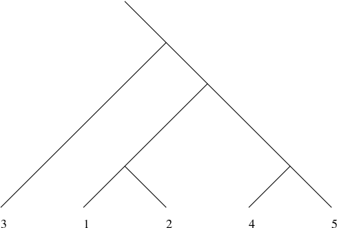
Some permutations will act trivially on some cladograms, such as the permutations $(12)(3)(45)$ and $(14)(25)(3)$ acting on the tree shown in Figure 2.

Let $S_{n}$ denote the permutation group of $[n]=\{1,2,\ldots,n\}$. In this case, the group action just defined extends uniquely, linearly, to an action of probabilities on $S_{n}$ upon probabilities on (fat or thin) cladograms. The action of the element $\frac{1}{n!}\sum_{\sigma\in S_{n}}\sigma$ will be of interest later on. This element has the effect of applying a uniform random permutation to the leaf labels of a cladogram.

This section covers the root join operation on trees, and the set of splits of a tree. The root join is used in the next chapter to define the alpha models. The splits of a tree are used to calculate the probability of a given tree under these models.

Informal definitions are given first, followed by more rigorous definitions and proofs.

If $t$ is a fat rooted binary tree which has left subtree $t_{1}$ and right subtree $t_{2}$ then $t$ may be thought of as the tree formed by joining together $t_{1}$ and $t_{2}$ at their roots. This is denoted $t_{1}*t_{2}=t$. See Figure 3 for an example.

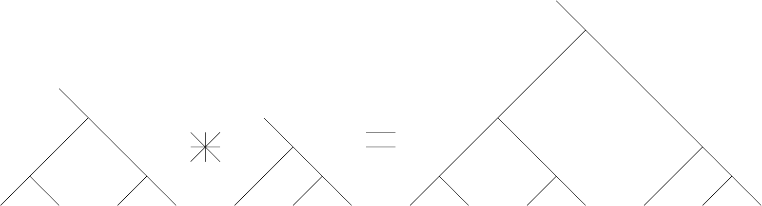
This construction also makes sense for thin (non-fat) trees and labeled trees, and this root join operation is preserved by the maps which forget orientation or leaf labels. Every binary tree is the root join of two subtrees in this way.

For thin trees $t_{1}*t_{2}=t_{2}*t_{1}$, but this is not true in general for fat trees.

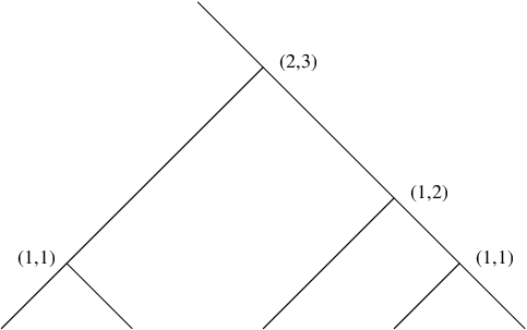
Splits are defined as follows. If $t=t_{1}*t_{2}$ and $t_{i}$ has $n_{i}$ leaves then say that the first split of $t$ is the ordered pair $(n_{1},n_{2})$ (or the unordered pair if $t$ is a thin tree). Similarly, each internal node has an associated split, as it is a branching point with some number of leaves below and to the left or right. The multiset (set with multiplicity) of splits of a tree is useful for calculating the probability of a tree under certain classes of self-similar probabilities. See Figure 4 for an example.

The definition of the subtree below an edge is useful in defining the root join operation.

See Figure 5 for and example.

Proof. First, show that the subtree of $t$ below edge $e$, call it $s$, is a tree. Let $e=\{v_{1},v_{2}\}$, with $v_{1}$ closer to the root of $t$, so that the root of $s$ is defined to be $v_{1}$. Any path in $s$ is a path in $t$ and so there is at most one path between any two vertices of $s$. On the other hand, every vertex of $s$ is either $v_{1}$ or a descendent of $v_{2}$ (ancestors and descendents referring to tree $t$). Every non self-intersecting path from a descendent of $v_{2}$ to $v_{2}$ passes through descendents of $v_{2}$ only. Since all descendents of $v_{2}$ lie in $s$ it follows that $s$ is connected. Thus $s$ is a tree. Finally, $v_{1}$ has degree $1$ in $s$, so $s$ is a rooted tree. $\Box$

This section contains the definition of the operation $\cdot*\cdot$ of joining two trees at the root. This operation is used extensively in the definitions to come so several of its properties are examined in detail.

Proof. If $t_{1}$ or $t_{2}$ is the empty tree then $t_{1}*t_{2}$ is equal to either $t_{2}$ or $t_{1}$ and so exists and is uniquely defined. Suppose now that $t_{1}$ and $t_{2}$ are non-empty trees.

Assume for the moment that $t_{1}$ and $t_{2}$ are thin, unlabeled rooted trees.

Let $t_{i}$ have vertex set $V_{i}$ and edge set $E_{i}$. Without loss of generality, suppose that the vertex sets of $t_{1}$ and $t_{2}$ intersect at a single element, $v_{0}$, which is the root for both trees. Let $r$ be an element not contained in $V_{1}$ or $V_{2}$. This will represent the root of the new tree.

Let $V=V_{1}\cup V_{2}\cup\{r\}$ and $E=E_{1}\cup E_{2}\cup\{\{v_{0},r\}\}$. Let $t$ be the graph with vertex set $V$ and edge set $E$. Now show that $t$ has the properties required of $t_{1}*t_{2}$.

First, show that $t$ is a tree. The graph $t$ is connected as there is a path from every vertex to the vertex $v_{0}$. Now to show that there is a unique non self-intersecting path between any two vertices. Note that $t_{1}$, $t_{2}$, and the graph $t_{3}$ with vertex set $V_{3}=\{v_{o},r\}$ and edge set $E_{3}=\{\{v_{0},r\}\}$ are all trees.

Any edge from a vertex in $V_{i}$ to a vertex in $V_{j}$, with $i\neq j$ must contain vertex $v_{0}$. Thus, any path from a vertex in $V_{i}$ to a vertex in $V_{j}$, with $i\neq j$ must pass through $v_{0}$. Thus, any non self-intersecting path from a vertex, $x$, in $V_{i}$ to a vertex, $y$, in $V_{j}$ must contain $v_{0}$ exactly once, with all vertices in the path before $v_{0}$ lying in $V_{i}$ and all those after $v_{0}$ lying in $V_{j}$. The sub-path from $x$ to $v_{0}$ in non self-intersecting and lies entirely in $V_{i}$ and so is unique, since $(V_{i},E_{i})$ is a tree. Similarly with the sub-path from $v_{0}$ to $y$. Thus the non self-intersecting path from $x$ to $y$ must be unique.

Any non self-intersecting path from a vertex $x$ to $y$, both in $V_{i}$, must lie entirely in $V_{i}$. Otherwise, if $v$ is any vertex in the path not lying in $V_{i}$ (and so not equal to $v_{0}$) then the sub-path from $x$ to $v$ passes through $v_{0}$ as does the sub-path from $v$ to $y$. Thus $v_{0}$ appears twice on a non self-intersecting path, which is a contradiction. Therefore, since the non self-intersecting path from $x$ to $y$ lies entirely in $V_{i}$ is must be unique, since $(V_{i},E_{i})$ is a tree.

Now show that $t$ has the required properties. First, It contains the required vertices, $r$,$v_{0}$,$v_{1}$,$v_{2}$, and edges, $\{r,v_{0},\}$,$\{v_{0},v_{1}\}$,$\{v_{0},v_{2}\}$, which are explicitly stated. Second, by the construction of $t$, for each $i=1,2$, the subtree of $t$ below edge $\{v_{0},v_{i}\}$ has vertex set $V_{i}$ and edge set $E_{i}$ and therefore is isomorphic to $t_{i}$.

Furthermore if $t_{1}$ and $t_{2}$ are fat rooted trees, with orientation functions $o_{1}$ an $o_{2}$, then let $t$ have orientation function $o$ defined by $o(r)=(v_{0})$, $o(v_{0})=(r,v_{0},v_{1})$ and $o(v)=o_{i}(v)$ for $v\in V_{i}\\ \{v_{0}\}$. Thus $t$ satisfies the additional requirements on the orientation of $t_{1}*t_{2}$.

Note that vertex $v$ is a (non-root) leaf of $t$ if and only if $v$ is a leaf of either $t_{1}$ or $t_{2}$.

Furthermore, if $t_{1}$ and $t_{2}$ are leaf-labeled trees then let $t$ be a leaf-labeled tree such that the leaf $v\in V_{i}\subset V$ of $t$ has the same label both as a vertex of $t$ and of $t_{i}$. All other vertices of $t$ are unlabeled. Thus $t$ satisfies the additional requirements on the labeling of $t_{1}*t_{2}$.

Next show that any two trees satisfying the definition of $t_{1}*t_{2}$ must be isomorphic. Again, begin by assuming simply that $t_{1}$ and $t_{2}$ are thin unlabeled rooted trees.

Let $s_{1}$ and $s_{2}$ be trees which satisfy the requirements of $t_{1}*t_{2}$. Therefore, $s_{i}$ contains vertices $r_{i},v_{i0},v_{i1},v_{i2}$ and edges $\{r_{i},v_{i0}\}$, $\{v_{i0},v_{i1}\}$, $\{v_{i0},v_{i2}\}$, such that $r_{i}$ is the root vertex of $s_{i}$ and, for each $j$ in $\{1,2\}$, the subtree of $t_{1}*t_{2}$ below edge $\{v_{i0},v_{ij}\}$ is isomorphic, via $f_{ij}$, to $t_{j}$.

Let $f$ be a map from the vertex set of $s_{1}$ to the vertex set of $s_{2}$ defined such that $f(r_{1})=r_{2}$, $f(v_{1j})=v_{2j}$ for $j=0,1,2$ and if $v$ is a descendent of $v_{1j}$ then $f(v)=f_{2j}^{-1}f_{1j}(v)$. This map is a bijection on vertices, sends the root to the root, and maps edges to edges, as does its inverse. Thus is it an isomorphism of thin rooted trees.

If $t_{1}$ and $t_{2}$ are both fat trees, or both leaf-labeled trees, then $f$ is also an isomorphism of, respectively, fat trees or leaf-labeled trees.

Thus there is exactly one tree, up to isomorphism, satisfying the requirements of $t_{1}*t_{2}$. $\Box$

Note that the sum of the number of leaves in two rooted trees is the same as the number of leaves in the root join of these two trees. In other words $|t_{1}*t_{2}|=|t_{1}|+|t_{2}|$.

Also, note that forgetting orientations before or after joining two trees at the root has the same effect. The same is true for forgetting leaf-labelings. Since this result is used often, it deserves a proposition.

Proof. This follows directly from the definitions for the binary operator $\cdot*\cdot$ and the forgetful maps $F_{o}$, which forgets orientations of fat trees, and $F_{l}$ which forgets labelings of labeled trees. $\Box$

The following result shows that there is only one way, up to isomorphism, to write a binary tree as the root join of two non-empty trees.

Proof. Suppose that $t$ is a non-empty rooted binary has more than $1$ leaf. Therefore $t$ has a root, $r$, which has a unique neighbor, $v_{0}$. This vertex, $v_{0}$, has degree $3$ and so has two distinct neighbors, $v_{1}$ and $v_{2}$, which are not the root $r$. If $t$ is a fat tree then choose $v_{1},v_{2}$ so that the orientation at $v_{0}$ is $(r,v_{1},v_{2})$. For $i=1,2$, let $t_{i}$ be the subtree of $t$ below edge $\{v_{0},v_{i}\}$. Thus the tree $t_{1}*t_{2}$ is exactly the tree $t$ (provided that the root vertex of $t_{1}*t_{2}$ is chosen to be the same element as the root vertex of $t$).

Suppose that $t$ is also equal to $t_{3}*t_{4}$. By the definition of the operation $\cdot*\cdot$, $t_{3}$ is isomorphic to the subtree of $t$ below edge $\{v_{0},v_{i}\}$ for some $i\in\{1,2\}$ and $t_{4}$ is isomorphic to the subtree of $t$ below the other edge $\{v_{0},v_{j}\}$, $j\in\{1,2\}$ such that $i\neq j$. Thus $t_{3}$ is isomorphic to one of $t_{1}$ or $t_{2}$, and $t_{4}$ is isomorphic to the other.

Furthermore, if $t$ is a fat tree then $t=t_{3}*t_{4}$ implies that $t_{3}$ is isomorphic to the subtree of $t$ below edge $\{v_{0},v_{1}\}$, which is $t_{1}$, and so the ordering of the two trees is also unique. $\Box$

Now for the formal definition of the splits of a tree. First, if $t$ is a binary rooted tree then let $|t|$ denote the number of leaves of $t$, also called the size of $t$.

Lemma 11 ensures that the first split is well defined.

Again, Lemma 11 ensures that this is well defined.

Equivalence of these definitions is not proven here.

The recursive definitions of alpha insertion for each type of tree are given below.

For the remainder of this section, let $s$ denote the one leaf binary rooted tree (tree shape), which is fat or thin as required by the context. This tree has two vertices and a single edge from the root vertex to the non-root leaf. Let $s_{x}$ be the one leaf binary rooted tree with leaf labeled $x$.

Let $|t|$ denote the number of leaves of a binary rooted tree $t$.

Uniqueness of the unordered pair $\{t_{1},t_{2}\}$ and commutativity of the root join operation on thin trees ensures that $i_{\alpha}$ is well defined in this case.

In other words, if $F_{l}$ is the function forgets leaf labels and $F_{o}$ is the function which forget orientations then

for trees $t$ of the appropriate type.

Proof. That alpha insertion commutes with forgetting orientations, $F_{o}$, follows directly from the definitions. The case of forgetting leaf labels follows by a simple induction.

For the initial case, $F_{l}(s_{x})=s$ and the root join operation is preserved by the map which forgets labels (Proposition 10). Thus, if $t$ is a single leaf tree then $F_{l}(i_{\alpha,x}(t))=F_{l}(\frac{1}{2}(t*s_{x}+s_{x}*t)=\frac{1}{2}(F_{l}(t)*F_{l}(s_{x})+F_{l}(s_{x})*F_{l}(t))=\frac{1}{2}(F_{l}(t)*s+s*F_{l}(t))=i_{\alpha}(F_{l}(t)$.

For the inductive step, if $t$ is not a single-leaf tree then $t=t_{1}*t_{2}$ for non-trivial trees $t_{1},t_{2}$. Assume the statement is true for all trees smaller than $t$, with fewer leaves that is. As $F_{l}$ respects $*$ it follows that $F_{l}(i_{\alpha,x}(t))$ is equal to

By the inductive assumption this is equal to

which is equal to $i_{\alpha}(F_{l}(t))$ as desired, since $F_{l}(t)=F_{l}(t_{1}*t_{2})=F_{l}(t_{1})*F_{l}(t_{2})$. $\Box$

The definitions of the alpha models for each of the four classes of trees are very similar. Each involves successive alpha insertions, of labeled or unlabeled leaves, and then a final uniform randomization of leaf labels in the labeled cases.

The definitions of the alpha models depend upon a single variable, usually called alpha or $\alpha$, which lies in the range $[0,1]$. Assume throughout that $\alpha$ is some fixed number.

Let $u_{n}=\frac{1}{n!}\sum_{\sigma\in S_{n}}\sigma$ be the uniform probability measure on the permutations of $[n]=\{1,2,\ldots,n\}$.

In other words, since $i_{\alpha,1}P_{0}=P_{1}$ is the unique measure on the single leaf tree, this definition says: start with the single leaf tree with leaf labeled $1$, alpha insert leaves labeled $2$ up to $n$ and then randomly permute the leaf labels.

Proof. The right hand side of the equation is equal to $u_{n}i_{\alpha,n}u_{n-1}i_{\alpha,n-1}\cdots i_{\alpha,1}P_{0}$. Since alpha insertion does not depend on the position of the labels of $t$, it follows that $i_{\alpha,n}u_{n-1}t=\sigma i_{\alpha,n}t$, where $\sigma$ is the image of $u_{n-1}$ under the usual injection of $S_{n-1}$ into $S_{n}$. Thus the right hand side is equal to $u_{n}\sigma i_{\alpha,n}i_{\alpha,n-1}\cdots i_{\alpha,1}P_{0}$ which is equal to $P_{n}$ as $u_{n}\sigma=u_{n}$ for any permutation $\sigma$. $\Box$

Define the alpha model on thin cladograms, fat tree shapes, and thin tree shapes to be the image of the alpha model on fat cladograms under the appropriate forgetful maps, $F_{o}$ and $F_{l}$ which forget orientations and leaf-labels respectively. Specifically:

Proof. Both of these propositions follow immediately from the previous two definition, and the fact that alpha insertion and the forgetful maps $F_{o}$ and $F_{l}$ ’commute’ (Proposition 18), and that $F_{l}(\sigma t)=F_{l}(t)$ for any fat or thin cladogram $t$ and any permutation, $\sigma$, of leaf labels. $\Box$

Markovian self-similarity basically means that the subtree below any edge is picked from the distribution on trees of the correct size, independently of the rest of the tree. It is also called Markov branching by Aldous in [4], as each branching happens independently of those above or on other paths from the root.

In other words, the trees below each child of the first branch-point are distributed independently from the same sequence of probabilities, conditional on the number of leaves they each have.

Call $q(\cdot,\cdot)$ the conditional split distribution of $(P_{n})_{n=1}^{\infty}$.

Must $q$ be unique?

Proof. In the case of fat rooted binary trees, $t_{1}*t_{2}=t_{3}*t_{4}$ if and only if $t_{1}=t_{3}$ and $t_{2}=t_{4}$. In particular, the number of leaves of $t_{1}$ is equal to the number of leaves of $t_{3}$, so $\sum_{m=1}^{n-1}q_{1}(m,n-m)P_{m}*P_{n-m}=\sum_{m=1}^{n-1}q_{2}(m,n-m)P_{m}*P_{n-m}$ if and only if $q_{1}=q_{2}$.

In the case of thin rooted binary trees, $t_{1}*t_{2}=t_{3}*t_{4}$ if and only if $t_{1}=t_{3}$ and $t_{2}=t_{4}$, or $t_{1}=t_{4}$ and $t_{2}=t_{3}$. In particular, the number of leaves of $t_{1}$ is equal to the number of leaves of either $t_{3}$ or $t_{4}$, so $\sum_{m=1}^{n-1}q_{1}(m,n-m)P_{m}*P_{n-m}=\sum_{m=1}^{n-1}q_{2}(m,n-m)P_{m}*P_{n-m}$ if and only if $q_{1}(m,n-m)+q_{1}(n-m,m)=q_{2}(m,n-m)+q_{2}(n-m,m)$.

References

- [1] David Aldous. The continuum random tree. I. Ann. Probab., 19(1):1–28, 1991.
- [2] David Aldous. The continuum random tree. II. An overview. In Stochastic analysis (Durham, 1990), volume 167 of London Math. Soc. Lecture Note Ser., pages 23–70. Cambridge Univ. Press, Cambridge, 1991.
- [3] David Aldous. The continuum random tree. III. Ann. Probab., 21(1):248–289, 1993.
- [4] David Aldous. Probability distributions on cladograms. In Random discrete structures (Minneapolis, MN, 1993), volume 76 of IMA Vol. Math. Appl., pages 1–18. Springer, New York, 1996.
- [5] David J. Aldous. Mixing time for a Markov chain on cladograms. Combin. Probab. Comput., 9(3):191–204, 2000.
- [6] David J. Aldous. Stochastic models and descriptive statistics for phylogenetic trees, from Yule to today. Statist. Sci., 16(1):23–34, 2001.
- [7] K. B. Athreya and P. E. Ney. Branching processes. Dover Publications Inc., Mineola, NY, 2004. Reprint of the 1972 original [Springer, New York; 0373040].
- [8] Krishna B. Athreya and Samuel Karlin. Embedding of urn schemes into continuous time Markov branching processes and related limit theorems. Ann. Math. Statist., 39:1801–1817, 1968.
- [9] A. Bagchi and A. K. Pal. Asymptotic normality in the generalized Pólya-Eggenberger urn model, with an application to computer data structures. SIAM J. Algebraic Discrete Methods, 6(3):394–405, 1985.
- [10] M. Blum and O. Francois. On statistical tests of phylogenetic imbalance: the sackin and other indices revisited.
- [11] M. Blum, O. Francois, and S. Janson. The mean, variance and joint distribution of two statistics sensitive to phylogenetic tree balance.
- [12] L.L. Cavalli-Sforza and A.W.F Edwards. Phylogenetic analysis. models and estimation proceduces. Am. J. Hum. Genet., 19:233–257, 1967.
- [13] D.H. Colless. Review of ”phylogenetics: the theory and practice of phylogenetic systematics.”. Sys. Zool, 31:100–104, 1982.
- [14] S.B. Heard. Patterns in tree balance among cladistic, phenetic and randomly generated phylogenetic trees. Evolution, 46:1818–1826, 1992.
- [15] S.B. Heard. Patterns in phylogenetic tree balance with variable and evolving speciation rates. Evolution, 50(6):2141–2148, 1996.
- [16] M. D. Hendy and David Penny. Branch and bound algorithms to determine minimal evolutionary trees. Math. Biosci., 59(2):277–290, 1982.
- [17] M. Kirkpartick and M. Slatkin. Searching for evolutionary patterns in the shape of a phylogenetic tree. Evolution, 46(4):1171–1181, 1993.
- [18] Andy McKenzie and Mike Steel. Distributions of cherries for two models of trees. Math. Biosci., 164(1):81–92, 2000.
- [19] A.O. Mooers and S.B. Heard. Inferring evolutionary process from phylogenetic tree shape. Quaterly Rev. Biology, 72(1):31–54, 1997.
- [20] A.O. Mooers, R.D.M. Page, A. Purvis, and P.H. Harvey. Phylogenetic noise leads to unblanaced cladistic tree reconstruction. Syst. Biol., 44:332–342, 1977.
- [21] J.S. Rogers. Response of tree imbalance to number of terminal taxa. Sys. Biol, 42(1):102–105, 1993.
- [22] J.S. Rogers. Central moments and probability distributions of three measures of phylogenetic tree imbalance. Sys. Biol, 45(1):99–110, 1996.
- [23] Uwe Rösler. A fixed point theorem for distributions. Stochastic Process. Appl., 42(2):195–214, 1992.
- [24] M.J. Sackin. ”good” and ”bad” phenograms. Sys. Zool, 21(2):225–226, 1972.
- [25] K.T. Shao and R. Sokal. Tree balance. Sys. Zool, 39(3):226–276, 1990.
- [26] R. T. Smythe. Central limit theorems for urn models. Stochastic Process. Appl., 65(1):115–137, 1996.
- [27] M. Steel and D. Penny. Distribution of tree comparison metrics some new results. System Biol., 42(2):126, 1993.
- [28] M. A. Steel. Distribution of the symmetric difference metric on phylogenetic trees. SIAM J. Discrete Math., 1(4):541–551, 1988.
- [29] Treebase. http://www.phylo.org/treebase/.
- [30] G.U. Yule. A mathematical theory of evolution : based on the conclusions of Dr. J.C. Willis, F.R.S. Harris and Sons, London, 1924.