Extremal properties of the determinant of the Laplacian in the Bergman metric on the moduli space of genus two Riemann surfaces

Any Riemann surface ${\cal L}$ from this family can be represented by the equation

$$y^{2}=(z^{2}-1)(z^{2}-r_{1}^{2})(z^{2}-r_{2}^{2})$$

(3.6)

where $r_{1},\,r_{2}\in{\mathbb{C}}$. In addition to the hyperelliptic involution there is an involution $\mu$ acting as $\mu:\;z\to-z$ on the curve (3.6).

The basic cycles on ${\cal L}$ chosen as shown in Fig. 3 transform as follows under the action of the involution $\mu$:

$$a_{1}^{\mu}=a_{2}\;\qquad b_{1}^{\mu}=b_{2}\;,$$

(3.7)

or equivalently,

$$\left(\begin{array}[]{cccc}b_{1}^{\mu}\\ b_{2}^{\mu}\\ a_{1}^{\mu}\\ a_{2}^{\mu}\end{array}\right)=T^{\mu}\left(\begin{array}[]{cccc}b_{1}\\ b_{2}\\ a_{1}\\ a_{2}\end{array}\right)$$

(3.8)

where the ${\rm Sp}(4,{\bf Z})$ matrix $T^{\mu}$ is given by

$$T^{\mu}=\left(\begin{array}[]{cccc}0&1&0&0\\ 1&0&0&0\\ 0&0&0&1\\ 0&0&1&0\end{array}\right)$$

(3.9)

Writing the matrix $T^{\mu}$ in block form:

$$T^{\mu}=\left(\begin{array}[]{cc}A^{\mu}&B^{\mu}\\ C^{\mu}&D^{\mu}\end{array}\right)$$

(3.10)

where $B^{\mu}=C^{\mu}=0$; $A^{\mu}=D^{\mu}=\left(\begin{array}[]{cc}0&1\\ 1&0\end{array}\right)$, and taking into account that, on one hand, the matrix of $b$-periods transforms under the action of any symplectic transformation as follows:

$${\bf B}\to{\bf B}^{\mu}:=(A^{\mu}{\bf B}+B^{\mu})(C^{\mu}{\bf B}+D^{\mu})^{-1}\;,$$

(3.11)

and that, on the other hand, the matrix of $b$-periods must remain invariant under the action of the biholomorphic transformation mapping the canonical basis of cycles to the new one, we conclude that ${\bf B}={\bf B}^{\mu}$. This is equivalent to

$${\bf B}=\left(\begin{array}[]{cc}0&1\\ 1&0\end{array}\right){\bf B}\left(\begin{array}[]{cc}0&1\\ 1&0\end{array}\right)\;;$$

thus the matrix ${\bf B}$ can be parametrized as follows:

$${\bf B}=\frac{1}{2}\left(\begin{array}[]{cc}{\bf x}+{\bf y}&{\bf x}-{\bf y}\\ {\bf x}-{\bf y}&{\bf x}+{\bf y}\end{array}\right)$$

(3.12)

If we factorize ${\cal L}$ with respect to the involution $\mu$, we get an elliptic curve ${\cal L}_{0}$ with period ${\bf y}$; ${\bf x}$ is the period of elliptic Prym variety corresponding to the (ramified) covering ${\cal L}\to{\cal L}_{0}$.

The description of the moduli space ${{{\cal M}}({\bf Z}_{2})}$ was given in [27] in terms of the variables $\tau_{1}={\bf y}$ and $\tau_{2}=-1/{\bf x}$. Below we describe this construction in terms of ${\bf x}$ and ${\bf y}$ themselves which makes it slightly more transparent. Denote by $\Gamma(2)$ the main congruence subgroup of $\Gamma$ consisting of matrices $\gamma$ such that $\gamma\equiv I\;({\rm mod}\;2)$ ($I$ is the unit matrix).

The natural idea of [27] is to reduce the action of the full group ${\rm Sp}(4,{\bf Z})$ on matrices of the form (3.12) to a correlated action of $\Gamma$ on ${\bf x}$ and ${\bf y}$.

Proof. The additional symmetries of the matrix $T\in{\rm Sp}(4,{\bf Z})$ (3.15) follow from the assumptions (3.7), (3.13) about the behavior of the basic cycles under the action of the involution $\mu$. The equivalence of the action of the matrix $T$ on the matrix (3.12) to the action of the two elements $\gamma_{1,2}$ (3.14) separately on ${\bf x}$ and ${\bf y}$ follows by direct computation. Finally the condition that all matrix entries of $T$ (3.15) are integer is equivalent to the condition that all matrix entries of the matrix $\gamma_{1}-\gamma_{2}$ are even. A simple computation using the conditions ${\rm det}\gamma_{i}=1$ shows that this is equivalent to the condition $\gamma_{1}\gamma_{2}^{-1}\in\Gamma(2)$ (which is more natural from the point of view of the group structure); it is straightforward to check that this condition is invariant under the natural group operation in $\Gamma\times\Gamma$.

$\square$

As was proved in [27], to get the full subgroup of ${\rm Sp}(4,{\bf Z})$ preserving the form (3.12) of the matrix of $b$-periods, one has to add to the subgroup (3.15) one more transformation, given by

$$T=\left(\begin{array}[]{cccc}1&0&0&0\\ 0&-1&0&0\\ 0&0&1&0\\ 0&0&0&-1\end{array}\right)$$

(3.16)

which maps the canonical basis $(b_{1},b_{2},a_{1},a_{2})$ to the basis $b_{1}^{\prime}=b_{1}\;,b_{2}^{\prime}=-b_{2}$, and $a_{1}^{\prime}=a_{1}\;,a_{2}^{\prime}=-a_{2}$; obviously, this transformation destroys the symmetry (3.7) of the canonical basis of cycles under the involution $\mu$. The action of the transformation (3.16) on the matrix of $b$-periods (3.12) is very simple: it changes the sign of the off-diagonal terms, i.e., it corresponds to the interchange of ${\bf x}$ and ${\bf y}$: ${\bf x}^{\prime}={\bf y}$, ${\bf y}^{\prime}={\bf x}$. Let us denote by $S_{2}$ the two-element permutation group generated by this transformation.

The theorem proved in [27] can now be reformulated as follows:

The subspace $\{({\bf x},{\bf y})\;|\;{\bf x}=\gamma{\bf y}\;,{\bf x},{\bf y}\in H\;,\;\gamma\in\Gamma(2)\}$ is taken out of $H\times H$ since it consists of matrices which are ${\rm Sp}(4,{\bf Z})$ equivalent to diagonal ones. The appearance of the group $G$ is explained above; Lemma 3.15 shows how to construct the natural group homomorphism $f$ from $G$ to ${\rm Sp}(4,{\bf Z})$.

The space ${\cal S}({\bf Z}_{2})$ (3.18) is called in [27] the “special Torelli space”, and the group $G$ (3.19) the “special Torelli group”.

The non-trivial part of the proof of this theorem (for which we refer the reader to [27]) is to show that no ${\rm Sp}(4,{\bf Z})$ transformation from the complement of the image of the homomorphism $f$ preserves the matrix of $b$-periods (3.12).

The structure of the fundamental domain ${{{\cal M}}({\bf Z}_{2})}$ (3.17) is rather non-trivial due to the necessity to take into account the subgroup $S_{2}$ interchanging ${\bf x}$ and ${\bf y}$. Therefore for our subsequent numerical analysis we introduce the “bigger” factor space $\Omega({\bf Z}_{2})=(H\times H)/G_{0}$, which can be easily described.

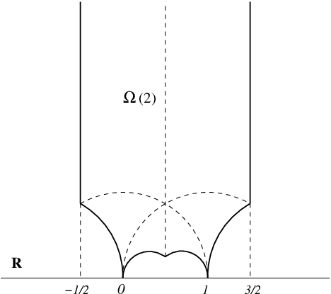
Proof is simple. To prove that any point $({\bf x},{\bf y})\in H\times H$ can be mapped to the inside of $\Omega\times\Omega(2)$ by some transformation from $G_{0}$, we first identify a $\gamma_{1}$ such that $\gamma_{1}{\bf x}\in\Omega$. As the second step we find a transformation $\gamma\in\Gamma(2)$ such that $\gamma(\gamma_{1}{\bf y})\in\Omega(2)$. Obviously the transformation mapping $({\bf x},{\bf y})$ to $(\gamma_{1}{\bf x},\,\gamma\gamma_{1}{\bf y})$ belongs to $G_{0}$ since $\gamma_{1}(\gamma\gamma_{1})^{-1}=\gamma^{-1}\in\Gamma(2)$.

Suppose now that some transformation $(\gamma_{1},\,\gamma_{2})\in G_{0}$ maps some point $({\bf x},{\bf y})\in\Omega\times\Omega(2)$ to another point $({\bf x}^{\prime},{\bf y}^{\prime})\in\Omega\times\Omega(2)$. Since $\gamma_{1}\in\Gamma$, it must be the identity element (since $\Omega$ is a fundamental domain for $\Gamma$). Therefore $\gamma_{2}\in\Gamma(2)$. Since $\gamma_{2}$ maps a point ${\bf y}\in\Omega(2)$ to another point ${\bf y}^{\prime}\in\Omega(2)$, $\gamma_{2}$ must also be the identity transformation.

$\square$

Curves of this family, which forms a subfamily of the two-parametric family (3.6), can be represented by the equation

$$y^{2}=z(z^{2}-1)(z^{2}-r^{2})$$

(3.21)

where $r\in{\mathbb{C}}$. In addition to the hyperelliptic involution, there are two more involutions: $\mu_{1}:\,z\to-z$ and $\mu_{2}:\,z\to r/z$ on the curve (3.21); the order of the full symmetry group $D_{2}\times{\bf Z}_{2}$ equals $8$.

Choose the branch cuts and basic cycles $(a_{i},b_{i})$ on ${\cal L}$ as shown in Fig. 6. The involutions $\mu_{1,2}$ act on this basis as follows:

$$b_{1}^{\mu_{1}}=b_{2}-a_{1}\;,\hskip 14.22636ptb_{2}^{\mu_{1}}=-b_{1}+a_{2}\;,\hskip 14.22636pta_{1}^{\mu_{1}}=a_{2}\;,\hskip 14.22636pta_{2}^{\mu_{1}}=-a_{1}\;,$$

(3.22)

and

$$b_{1}^{\mu_{2}}=b_{2}\;,\hskip 14.22636ptb_{2}^{\mu_{2}}=b_{1}\;,\hskip 14.22636pta_{1}^{\mu_{2}}=a_{2}\;,\hskip 14.22636pta_{2}^{\mu_{2}}=a_{1}\;;$$

(3.23)

therefore the action of $\mu_{1}$ and $\mu_{2}$ on the vector $(b_{1},\,b_{2},\,a_{1},\,a_{2})^{t}$ is given by the following ${\rm Sp}(4,{\bf Z})$ matrices:

$$T^{\mu_{1}}=\left(\begin{array}[]{cccc}0&1&-1&0\\ -1&0&0&1\\ 0&0&0&1\\ 0&0&-1&0\end{array}\right)\;;\qquad T^{\mu_{2}}=\left(\begin{array}[]{cccc}0&1&0&0\\ 1&0&0&0\\ 0&0&0&1\\ 0&0&1&0\end{array}\right)\;,$$

(3.24)

respectively. Invariance of the matrix of $b$-periods under the ${\rm Sp}(4,{\bf Z})$ transformation defined by $T^{\mu_{1}}$ implies the following structure of the matrix in the chosen basis:

$${\bf B}=\left(\begin{array}[]{cc}\sigma&1/2\\ 1/2&\sigma\end{array}\right)$$

(3.25)

where $\sigma\in{\mathbb{C}}$; $\Im\sigma>0$. Invariance of the matrix of $b$-periods under the action of $T^{\mu_{2}}$ does not impose any other restriction.

It will be convenient for us to work in terms of the parameter ${\bf x}=\sigma+1/2$, i.e., to represent the matrix ${\bf B}$ in the form

$${\bf B}=\left(\begin{array}[]{cc}{\bf x}-1/2&1/2\\ 1/2&{\bf x}-1/2\end{array}\right)$$

(3.26)

for $\Im{\bf x}>0$. The moduli space ${\cal M}(D_{2})$ of $D_{2}$ curves can be realized as the upper complex half-plane in the variable ${\bf x}=\sigma+1/2$ factorized with respect to the action of the group ${\rm Sp}(4,{\bf Z})$ on matrices of the form (3.26).

The analogue of Schiller’s theorem 2 for the $D_{2}$ family looks as follows. Let us introduce the modular group $\Gamma_{0}(2)$ which is the subgroup of $SL(2,{\bf Z})$ consisting of matrices whose $(21)$ entry is even. The minimal subgroup of $GL(2,{\bf Q})$ containing $\Gamma_{0}(2)$ and the element

$$\left(\begin{array}[]{cc}0&-1\\ 2&0\end{array}\right)$$

is called $\Gamma_{0}(2)+$. The group $\Gamma_{0}(2)+$ is generated by the following two elements [8, 7]:

$$\gamma_{1}=\left(\begin{array}[]{cc}1&1\\ 0&1\end{array}\right)\;\qquad{\rm and}\qquad\gamma_{2}=\left(\begin{array}[]{cc}2&-1\\ 2&0\end{array}\right)\;.$$

(3.27)

Proof. The proof can be obtained as a corollary of Schiller’s theorem 2. To restrict ${\cal M}({\bf Z}_{2})$ to ${\cal M}(D_{2})$ one should put ${\bf y}={\bf x}-1$. It is straightforward to verify that the subgroup of the group $G$ (3.19) preserving the constraint ${\bf y}={\bf x}-1$ coincides with $\Gamma_{0}(2)+$.

In particular, the action of the generators $\gamma_{1}$ and $\gamma_{2}$ on ${\bf x}$ is equivalent to the action of the following matrices $T_{1,2}\in{\rm Sp}(4,{\bf Z})$ on the matrix (3.26), respectively:

$$f(\gamma_{1}):=T_{1}=\left(\begin{array}[]{cccc}1&0&1&0\\ 0&1&0&1\\ 0&0&1&0\\ 0&0&0&1\end{array}\right)\;,\hskip 28.45274ptf(\gamma_{2}):=T_{2}=\left(\begin{array}[]{cccc}0&-1&1&0\\ 0&-1&0&0\\ -1&-1&0&0\\ 1&-1&1&-1\end{array}\right)\;.$$

(3.30)

This defines the group homomorphism $f:\Gamma_{0}(2)+\to{\rm Sp}(4,{\bf Z})$ on the generators of $\Gamma_{0}(2)+$ which extends to the whole group according to the group structure.

It remains to understand which matrices of the form (3.26) are ${\rm Sp}(4,{\bf Z})$-equivalent to diagonal ones. Since it is not obvious to get this information from Schiller’s theorem 2, we choose an indirect way. First, applying the transformation

$$\left(\begin{array}[]{cccc}0&1&0&0\\ 0&1&-1&0\\ -1&0&0&1\\ 1&0&0&0\end{array}\right)$$

to the matrix (3.25) with ${\bf x}=1/2+i/2$, we get the diagonal matrix ${\rm diag}(i,\;i)$. Therefore, this vertex of the fundamental domain $\Omega_{0}(2)+$ (as well as any point equivalent to this point under $\Gamma_{0}(2)+$ transformations), corresponds to a degeneration of a genus two Riemann surface to the union of two tori. On the other hand, the moduli space ${\cal M}(D_{2})$ can be alternatively parametrized by $\alpha^{2}$, where $\alpha$ is the coefficient of the sextic $xy(x^{4}+\alpha x^{2}y^{2}+y^{4})$ (this form of equation can be obtained by a simple transformation from (3.21)); all values of $\alpha^{2}$ correspond to different points of ${\cal M}(D_{2})$. In terms of $\alpha^{2}$ the space ${\cal M}(D_{2})$ looks like the Riemann sphere with two deleted points: $\alpha^{2}=\infty$, and $\alpha^{2}=4$, where the Riemann surface degenerates [9]. Since we already know two degeneration points in terms of the parameter ${\bf x}$ (${\bf x}=i\infty$ and ${\bf x}=1/2+i/2$, which correspond to $\alpha^{2}=\infty$ and $\alpha^{2}=4$, respectively), we can conclude that these are the only boundary points of ${\cal M}(D_{2})$ in $\Omega_{0}(2)+$.

Therefore, all matrices of the form (3.25) which are ${\rm Sp}(4,{\bf Z})$-equivalent to diagonal ones, can be obtained from the value ${\bf x}=1/2+i/2$ by a $\Gamma_{0}(2)+$ transformation.

$\square$

Now we can identify the space ${\cal M}(D_{2})$ with the fundamental domain $\Omega_{0}(2)+$ of the group $\Gamma_{0}(2)+$ (see Fig.7). The vertical lines are identified by the transformation $\gamma_{1}$ from (3.27); the arcs are identified by the transformation $\gamma_{2}$ from (3.27).

The space ${\cal S}(D_{2})$ (3.29) is the natural analog of the Torelli space for the $D_{2}$ family (the “special $D_{2}$ Torelli space”); the group $\Gamma_{0}(2)+$ can be naturally called the “special $D_{2}$ Torelli group”, in analogy to Schiller’s terminology for the case of ${\cal M}({\bf Z}_{2})$.

This is another subfamily of the two-parametric family (3.6) [3]. Curves admitting this symmetry group also form a one-parametric sub-family of (3.6); they can be represented by the equation

$$y^{2}=(z^{3}-1)(z^{3}-r^{3})$$

(3.31)

where $r\in{\mathbb{C}}$. In addition to the hyperelliptic involution two more generators of the symmetry group are acting on the curve (3.31): the element of order three $\mu_{1}:z\to\epsilon_{3}z$ and the involution $\mu_{2}:z\to r/z$; the order of the full symmetry group $D_{3}\times{\bf Z}_{2}$ equals $12$.

Choose the branch cuts and basic cycles $(a_{i},b_{i})$ on ${\cal L}$ as shown in Fig. 8. The symmetries $\mu_{1,2}$ act on this basis as follows:

$$b_{1}^{\mu_{1}}=b_{2}-b_{1}\;,\hskip 14.22636ptb_{2}^{\mu_{1}}=-b_{1}\;,\hskip 14.22636pta_{1}^{\mu_{1}}=a_{2}\;,\hskip 14.22636pta_{2}^{\mu_{1}}=-a_{1}-a_{2}\;;$$

(3.32)

and

$$b_{1}^{\mu_{2}}=b_{1}-b_{2}\;,\hskip 14.22636ptb_{2}^{\mu_{2}}=-b_{2}\;,\hskip 14.22636pta_{1}^{\mu_{2}}=a_{1}\;,\hskip 14.22636pta_{2}^{\mu_{2}}=-a_{1}-a_{2}\;;$$

(3.33)

therefore the action of $\mu_{1}$ and $\mu_{2}$ on the vector $(b_{1},\,b_{2},\,a_{1},\,a_{2})^{t}$ is given by the following ${\rm Sp}(4,{\bf Z})$ matrices:

$$T^{\mu_{1}}=\left(\begin{array}[]{cccc}-1&1&0&0\\ -1&0&0&0\\ 0&0&0&1\\ 0&0&-1&-1\end{array}\right)\;;\qquad T^{\mu_{2}}=\left(\begin{array}[]{cccc}1&-1&0&0\\ 0&-1&0&0\\ 0&0&1&0\\ 0&0&-1&-1\end{array}\right)\;,$$

(3.34)

respectively.

Invariance of the matrix of $b$-periods under the transformation defined by $T^{\mu_{1}}$ implies its following structure in the chosen basis:

$${\bf B}=\left(\begin{array}[]{cc}2\sigma&\sigma\\ \sigma&2\sigma\end{array}\right)$$

(3.35)

where $\sigma\in{\mathbb{C}}$; $\Im\sigma>0$. Invariance of the matrix of $b$-periods matrix under the action of $T^{\mu_{2}}$ does not impose any other restriction.

Introduce the subgroup $\Gamma_{0}(3)$ of $SL(2,{\bf Z})$, which consists of matrices whose $(21)$ matrix entry $\equiv 0\;(mod\;\;3)$. The minimal subgroup of $GL(2,{\bf Q})$ containing both $\Gamma_{0}(3)$ and the matrix

$$\left(\begin{array}[]{cc}0&-1\\ 3&0\end{array}\right)$$

is called $\Gamma_{0}(3)+$. The group $\Gamma_{0}(3)+$ is generated by the following two elements:

$$\gamma_{1}=\left(\begin{array}[]{cc}1&1\\ 0&1\end{array}\right)\;,\hskip 28.45274pt\gamma_{2}=\left(\begin{array}[]{cc}3&-1\\ 3&0\end{array}\right)\;;$$

(3.36)

Proof. The proof can be obtained as a corollary of Schiller’s theorem 2. To restrict ${\cal M}({\bf Z}_{2})$ to ${\cal M}(D_{3})$ one should put ${\bf x}=3\sigma$, ${\bf y}=\sigma$. It is straightforward to verify that the subgroup of the group $G$ (3.19) preserving the constraint ${\bf x}=3{\bf y}$ coincides with $\Gamma_{0}(3)+$ acting on $\sigma(\equiv{\bf y})$.

In particular, the action of the generators $\gamma_{1}$ and $\gamma_{2}$ on $\sigma$ is equivalent to the action of the following ${\rm Sp}(4,{\bf Z})$ matrices $T_{1,2}\in{\rm Sp}(4,{\bf Z})$ on the matrix of $b$-periods (3.35), respectively:

$$f(\gamma_{1}):=T_{1}=\left(\begin{array}[]{cccc}1&0&2&1\\ 0&1&1&2\\ 0&0&1&0\\ 0&0&0&1\end{array}\right)\;,\hskip 28.45274ptf(\gamma_{2}):=T_{2}=\left(\begin{array}[]{cccc}-2&1&1&0\\ -1&2&0&-1\\ -1&0&0&0\\ 0&1&0&0\end{array}\right)\;,$$

This defines the group homomorphism $f:\Gamma_{0}(3)+\to{\rm Sp}(4,{\bf Z})$ on the generators of $\Gamma_{0}(3)+$ which extends to the whole group according to the group structure.

It remains to understand which matrices of the form (3.35) are ${\rm Sp}(4,{\bf Z})$- equivalent to diagonal ones. Again, it is not obvious to get this information from Schiller’s theorem 2, and we shall use well-known facts about the structure of ${\cal M}(D_{3})$ in terms of the coefficients of the sextic.

First, applying the transformation

$$\left(\begin{array}[]{cccc}0&1&0&0\\ 0&1&-1&0\\ -1&0&0&1\\ 1&0&0&0\end{array}\right)$$

to the matrix (3.35) with ${\bf x}=1/2+i/2\sqrt{3}$, we get the diagonal matrix ${\rm diag}(-\frac{1}{2}+\frac{i\sqrt{3}}{2},\;\frac{1}{2}+\frac{i\sqrt{3}}{2})$. Therefore, this point (as well as any point equivalent to this point under $\Gamma_{0}(3)+$ transformations), corresponds to a degeneration of a genus two Riemann surface to the union of two tori.

On the other hand, the moduli space ${\cal M}(D_{3})$ can be alternatively parametrized by $\alpha^{2}$, where $\alpha$ is the coefficient of the sextic $x^{6}+\alpha x^{3}y^{3}-y^{6}$ (this form of the equation can be obtained by a simple transformation from (3.31)); all values of $\alpha^{2}$ correspond to different points of ${\cal M}(D_{2})$. In terms of $\alpha^{2}$ the space ${\cal M}(D_{3})$ looks like the Riemann sphere with two deleted points: $\alpha^{2}=\infty$, and $\alpha^{2}=-4$, where the Riemann surface degenerates [9]. Since we already know two degeneration points in terms of the parameter ${\bf x}$ (${\bf x}=i\infty$ and ${\bf x}=1/2+i/2\sqrt{3}$, which correspond to $\alpha^{2}=\infty$ and $\alpha^{2}=-4$, respectively), we can conclude that these are the only boundary points of ${\cal M}(D_{3})$ in $\Omega_{0}(3)+$.

Therefore, all matrices of the form (3.35) which are ${\rm Sp}(4,{\bf Z})$- equivalent to a diagonal one, can be obtained from the value ${\bf x}=1/2+i/2\sqrt{3}$ by a $\Gamma_{0}(3)+$ transformation.

References

- [1] T. Apostol, Modular functions and Dirichlet series in number theory, Graduate Texts in Mathematics, No. 41. Springer, New York-Heidelberg (1976)
- [2] A. Ash, On the existence of eutactic forms, Bull. London Math.Soc. 12 192-196 (1980)
- [3] O. Bolza, On binary sextics with linear transformations into themselves, Amer. J. Math. 10 47-60 (1888)
- [4] J.-B. Bost, J.-F. Mestre, L. Moret-Bailly, Sur le calcul explicite des “classes de Chern” des surfaces arithmétiques de gendre 2, Astérisque 183 69-105 (1990)
- [5] J. Bryan, J. Fulman, Orbifold Euler characteristics and the number of commuting -tuples in the symmetric group, math.CO/9712248
- [6] P. Buser, R. Silhol, Geodesics, periods and equations of real hyperelliptic curves, Duke Math. J, 108, 211Ð250 (2001)
- [7] C. Cummins, private communication
- [8] L. R. Ford, Automorphic functions, McGraw-Hill, New York (1929)
- [9] E. Getzler, Euler characteristics of local systems on , Compositio Mathematica 132 121-135 (2002)
- [10] E. Gottschling, Explizite Bestimmung der Randflächen des Fundamentalbereiches der Modulgruppe zweiten Grades. Math. Ann. 138 103-124 (1959)
- [11] J. Harer, D. Zagier, The Euler characteristic of the moduli space of curves, Invent. Math., 85 457-485 (1986)
- [12] F. Hirzebruch, T. Höfer, On the Euler number of an orbifold, Math.Ann., 286 255-260 (1990)
- [13] J. Igusa, Arithmetic variety of moduli for genus two, Ann. of Math. (2) 612-649 72 (1960)
- [14] D. Jakobson, M. Levitin, N. Nadirashvili, N. Nigam, I. Polterovich, How large can the first eigenvalue be on a surface of genus two? math.SP/0509398. Intern.Math.Res.Notices, to appear
- [15] V. Knizhnik, Multiloop amplitudes in the theory of quantum strings and complex geometry, Soviet Phys. Uspekhi 32 945-971 (1989)
- [16] M. Kontsevich, A. Zorich, Connected components of the moduli spaces of holomorphic differentials with prescribed singularities, Invent. Math. 153 631-678 (2003)
- [17] A. Kokotov, D. Korotkin Isomonodromic tau-function of Hurwitz Frobenius manifolds and its applications, math-ph/031008
- [18] A. Kokotov, D. Korotkin, “Normalized Ricci flow and determinant of Laplacian”, Lett. Math. Phys., 71 241-242 (2005)
- [19] A. Kokotov, D. Korotkin, Tau-functions on spaces of Abelian differentials and higher genus generalizations of Ray-Singer formula, preprint of MPI Leipzig, 46/2004
- [20] J. C. Lagarias, , J. A. Reeds, M. H. Wright, and P. E. Wright, Convergence Properties of the Nelder-Mead Simplex Method in Low Dimensions, SIAM J. Optim., 9 N.1, 112-147 (1998)
- [21] B. Osgood, R. Phillips, P. Sarnak, Extremals of determinants of Laplacians. J. Funct. Anal. 80 148-211 (1988)
- [22] M. Pollicott, A. Rocha, A remarkable formula for the determinant of the Laplacian. Invent. Math. 130 399-414 (1997)
- [23] E. Rauch, J. Lewittes, The Riemann surface of Klein with 168 automorphisms, in Problems in analysis (papers dedicated to S.Bochner), 297-308 Princeton Univ. Press (1970)
- [24] D. B. Ray, I. M. Singer, Analytic torsion for complex manifolds. Ann. Math. (2) 98, 154–177 (1973)
- [25] J. R. Quine and P. Sarnak, eds., Extremal Riemann surfaces, Contemporary Mathematics, 201 AMS (1997)
- [26] P. Sarnak, Extremal geometries, in [25]
- [27] J. Schiller, Moduli for special Riemann surfaces of genus two, Trans. Amer. Math. Soc. 144 95-113 (1969)
- [28] P. Schmutz Schaller, Geometry of Riemann surfaces based on closed geodesics, Bulletin AMS 35 No.3 193-214 (1998)
- [29] P. Schmutz Schaller, Systoles and topological Morse functions for Riemann surfaces, J. Diff. Geom. 52 407-452 (1999)
- [30] C. L. Siegel, Symplectic geometry. Academic Press, New York-London (1964)
- [31] R. Silhol, Period matrices and the Schottky problem, in Topics on Riemann surfaces and Fuchsian groups 155-163, London Math. Soc. Lecture Note Ser., 287 Cambridge Univ. Press (2001)
- [32] W. Thurston, Geometry and topology of 3-manifolds, Princeton lectures (1978)
- [33] K. Yoshikawa, Discriminants of theta divisors and Quillen metrics, J. Diff. Geom. 52 73-115 (1999)