A Numerical Examination of the Castro-Mahecha Supersymmetric Model of the Riemann Zeros
Abstract
The unknown parameters of the recently-proposed (Int J. Geom. Meth. Mod. Phys. 1, 751 [2004]) Castro-Mahecha model of the imaginary parts () of the nontrivial Riemann zeros are the phases () and the frequency parameter () of the Weierstrass function of fractal dimension and the turning points () of the supersymmetric potential-squared — which incorporates the smooth Wu-Sprung potential (Phys. Rev. E 48, 2595 [1993]), giving the average level density of the Riemann zeros. We conduct numerical investigations to estimate/determine these parameters — as well as a parameter () we introduce to scale the fractal contribution. Our primary analyses involve two sets of coupled equations: one set being of the form , and the other set corresponding to the fractal extension — according to an ansatz of Castro and Mahecha – of the Comtet-Bandrauk-Campbell (CBC) quasi-classical quantization conditions for good supersymmetry, . Our analyses suggest the possibility strongly that converges to its theoretical lower bound of 1, and the possibility that all the phases () should be set to zero. We also uncover interesting formulas for certain fractal turning points.
Keywords:
Riemann zeros, Wu-Sprung potential, Weierstrass fractal function, supersymmetry, Castro-Mahecha model, Comtet-Bandrauk-Campbell (CBC) formula, turning points, Riemann Hypothesis, simultaneous nonlinear equations, Brownian motionpacs
Valid PACS 02.10.De, 03.65.Sq, 05.45.Df, 11.30.PbI Introduction
The precise nature of the zeros of the Riemann zeta function is of paramount mathematical Conrey 2003, as well as physical interest Bunimovich and Dettmann 2005. Of course, perhaps the most famous, not yet fully resolved, mathematical conjecture (the Riemann Hypothesis Rockmore 2005) is that all the nontrivial zeros () — the trivial zeros simply equalling , — have real components .
Castro and Mahecha Castro and Mahecha 2004 recently proposed a supersymmetric implementation of the Wu-Sprung model Wu and Sprung 1993 of the ’s, employing a Weierstrass (continuous and nowhere differentiable) function Berry and Lewis 1980 for the fractal structure of dimension that Wu and Sprung had found for their local one-dimensional potential () (cf. Khuri 2002; Rosu 2003). The Wu-Sprung potential — which generates the smooth average level density obeyed by the Riemann zeros — satisfied Abel’s integral equation (Wu and Sprung 1993, eq. (6)), and was written implicitly as (Wu and Sprung 1993, eq. (7)),
| (1) |
Here .
The Weierstrass fractal function employed by Castro and Mahecha (Castro and Mahecha 2004, eq. (81)),
| (2) |
has both an unknown (countably) infinite set of phases and an unknown parameter , which determines the frequencies . Further, is the fractal dimension, which Castro and Mahecha — following the box-counting argument of Wu and Sprung Wu and Sprung 1993 (cf. van Zyl and Hutchinson 2003) — took to be . (Castro and Mahecha also noted (Castro and Mahecha 2004, sec. 6) that this choice of does, appealingly, yield [the omnipresent] noise.) The variable parameterizes the inverted Wu-Sprung potential , which in accordance with the supersymmetric requirement that the energy be zero in the ground state, was translated to be zero at .
Rather than directly addressing the formidable problem “of factoring the ordinary Schrödinger equation studied by Wu-Sprung”, Castro and Mahecha (CM) postulated the model (Castro and Mahecha 2004, eq. (82)),
| (3) |
with
| (4) |
( denotes complex conjugation.) The additive constant is chosen so that, in accordance with supersymmetric principles, . The “turning points” (where the potential energy is equal to the total energy), along with the phases and the parameter , are the unknown (countably infinite) parameters of the CM model, which we hope here to estimate/determine, by satisfying the equations (3), simultaneously with the quantization conditions (Castro and Mahecha 2004, eq. (87)),
| (5) |
Castro and Mahecha proposed (cf. (Laskin 2002, eq. (36))) that these relations would constitute the fractal extension of the fermionic phase path integral approximation (the CBC [Comtet-Bandrauk-Campbell] formula (cf. (Inomata and Junker 1994, eq. (1)) (Wu and Sprung 1993, eq. (5)))) — the supersymmetric counterpart of the well-known WKB quantization rule (Inomata and Junker 1994, eq. (2)). Here and runs over the positive integers.
The Castro-Mahecha model (3) was cast in a fractal supersymmetric quantum-mechanical (SUSY-QM) setting, in an effort to implement the Hilbert-Polya proposal Edwards 1974 to prove the Riemann Hypothesis, under which an Hermitian operator, hypothetically, can be found to reproduce the ’s as its spectrum. It had appeared to CM quite difficult to directly solve the SUSY Schrödinger equation (Castro and Mahecha 2004, eq. (84)),
| (6) |
where , , the are eigenfunctions, and the fractional derivative
| (7) |
is intended (cf. Laskin 2002). (M. Trott suggested that one might directly pursue the solution of this system, most effectively, using a Grünwald-Letnikov discrete approximation Ma and Hori 2003.) CM, therefore, had recourse to the CBC formula (5) as an approximation to the implementation of the quantum inverse scattering method, which would yield the potential . Given an exact potential, one could construct the SUSY Schrödinger equation, giving the ’s for its eigenvalues. This would realize — CM claimed — the Hilbert-Polya proposal to prove the Riemann Hypothesis.
CM reasoned that if the potential energy has the shape of a fractal curve, then it is very natural to assume that the kinetic energy operator should be a fractal; namely it should be expressed in terms of fractal derivatives.
In sec. II, we begin our numerical analyses by studying the solutions to (3). Then, in sec. III, we extend the analyses to include (simultaneously) the two sets of equations (3) and (5). The fractal Wu-Sprung potential is examined in sec. IV, in particular its turning points, for a number of which interesting formulas are obtained. In sec. V, we expand the CM model to include a certain scaling factor. A discussion of our analyses is contained in sec. VI. We also include an Appendix outlining recent work of D. Dominici concerning the inversion of the Wu-Sprung potential Dominici.
II Preliminary analyses
II.1 Turning points — for smooth potential — held fixed
Our initial numerical analyses of the CM model consisted of, for various integral cut-offs on the running index in the Weierstrass fractal function summation (2), finding an optimizing set of ’s, while keeping the ’s fixed and equal to ( of) the turning points for the translated inverted smooth Wu-Sprung potential, that is, those ’s for which (cf. (3)),
| (8) |
The set of estimated ’s and would be chosen, so as to minimize the sum of squared deviations — since it did not appear possible to achieve complete equality — between the LHS (left-hand side) and RHS of (8). Computationally-speaking we employed the NMinimize command of Mathematica, using the “DifferentialEvolution” and “InitialPoints” options, and for the initial points only increasing sets of values for the ’s, in order to reduce search times. Also, the necessary inversion of the Wu-Sprung potential (1) — in order to obtain — was performed using the Interpolation command of Mathematica (cf. Appendix).
We, first, found certain evidence, at least in this initial context, that suggested taking . (In Castro and Mahecha 2004, CM wrote that “it would be intriguing to see if , the inverse of the golden mean, since the golden mean appears in the theory of quantum noise related to the Riemann Hypothesis” (cf. (Berry and Lewis 1980, p. 481)).
Initially, we tried the case , insisting that the phases be ordered from lowest to highest. Our results were encouraging, and we proceeded to successively higher integral values of , reaching . (We make the obvious comment that here the number of unknowns [] equals the number of [nonlinear] equations.) For that case, the best fit to the first 100 ’s yielded a remarkably small sum-of-squares deviations of . The first seventy-seven of the hundred ordered phases (that is, ) were all equal to to, typically, seven decimal places (Fig. 1).

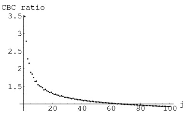
When we inserted the turning points () derived from the (smooth) inverted Wu-Sprung potential for the bounds of integration — that is, those satisfying (8) — into the fractal CBC formula (5), we found that these quantization relations were clearly not fully met. (In general, the CBC quantization conditions appear to hold for a number of “shape-invariant” potentials Inomata and Junker 1994 (cf. Bhaduri et al. 2005).) In Fig. 2, we plot the (CBC) ratio of the computed value of the real part of the LHS of (5) to its RHS (that is, ). We see that for the lower values of , the LHS’s exceed , while for the higher values, they are less than — all in an apparently smooth monotonically decreasing manner.
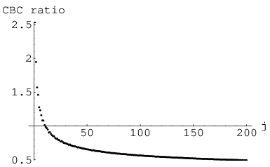
We, then, were able to extend our computer analyses to the case , with very analogous results (Fig. 3). (The sum of squared deviations was quite small, as in the analysis, .) Most of the estimated values of were once again to high precision, this time for .

In regard to the phases of the Weierstrass fractal function, Castro and Mahecha (Planat and Rosu 2003, sec. 5) had written that it “is warranted to see if the statistical distribution of these phases has any bearing to random matrix theory (the circular unitary random matrix ensemble) and the recent studies of quantum phase-locking, entanglement, Ramanujan sums and cyclotomy studied by Planat and Rosu 2003”.
When we proceeded to the still higher-order case , we found
superficially, at least, different types of results.
In six different runs (using different random seeds)
of our Mathematica program, we obtained sum-of-squares deviations
no greater than
, all six yielding essentially the
same-looking plot. The smallest sum-of-squares was ,
corresponding to Fig. 5.

The first seventy-four scaled phases () were all equal to (rather than , as previously) to high accuracy. Let us note, in any case though, that for either or , the factors in the expansion (2) of the Weierstrass fractal function have zero real part.
II.2 Comment
What it appeared, in retrospect, we had actually principally accomplished above (Figs. 1, 3, 5) was to find sets of phases () for various (100, 200 and 300), such that the real part of the Weierstrass fractal function (2) is very close to zero — as revealed by plots — for any (or ), be it a turning point or not. So, these results immediately pertain to the Weierstrass fractal function and not the Riemann zeros themselves. Nevertheless, our estimated phases (’s) can be employed as the first step of an iterative procedure — as discussed in the next section.
Since the Castro-Mahecha supersymmetric model of the Riemann zeros requires the simultaneous obtaining/fitting of phases (’s), the parameter , and turning points (’s), we turn to this problem now.
III Joint Estimation of Phases () and Turning Points ()
III.1 Iterative approach
III.1.1 analyses
We would like now to regard the two sets of equations (3) — the one set we have tried to satisfy in the above analyses — and (5) as a coupled system and attempt to simultaneously solve for the phases () and turning points () (still holding ). In this context, we again considered the case , and took the solution portrayed in Fig. 1 as the first step of an iterative procedure. Using this set of ’s, we searched for a new set of turning points (), such that the CBC quantization conditions (5) would all be exactly (up to our numerical accuracy) satisfied. Then, with this revised set of ’s, we hoped to find anew the set of ’s satisfying (3). By reiterating this two-step procedure a sufficiently large number of times, we anticipated possibly arriving at a final set of ’s and ’s simultaneously satisfying (3) and (5) (cf. Rüschendorf 1995). A test for convergence to such a final solution would be that the two sets of parameters would only change negligibly upon further iterations. 11 1 M. Trott suggested — in analogy to the self-consistent solution of Schrödinger and Poisson equations for some charged system — that it might be a more superior/stable iterative scheme, to at each stage combine the current, revised estimates of the ’s and ’s with those from the preceding step of the iterative procedure, in fact, perhaps much more strongly weighting the preceding () estimates. We have not yet thoroughly pursued this possibility, though.
At the very beginning of the iterative procedure we have just outlined, we sought to obtain a (hypothetical, second) set of one hundred turning points (), which would render the CBC quantization conditions (5) completely satisfied when the first set of phases () — those depicted (in their scaled form) in Fig. 1 — were employed. However, this proved to be not totally doable. For example, for the original value of , the corresponding CBC ratio was 0.926293. But when we tried to adjust to increase this ratio closer to the ideal value of 1, we were only able to obtain a slight improvement by going to , for which the ratio was 0.937452. We show this phenomenon in Fig. 6.

In all one hundred cases, when we sought to drive the CBC ratios closer to unity, the new turning points chosen, , were smaller than the originals (Fig. 7).

(There is some anomalous behavior apparent, in that .) For the first seventy-one cases, the new turning points () do yield the desired CBC ratio of 1 (Fig. 8). (We have not been able to obtain a revised set of ’s based on the 100 ’s to closely satisfy (3), as we had with the 100 ’s.)

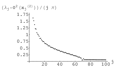
When the revised set of turning points was employed, along with the original set of phases ’s (Fig. 1), instead of highly accurate predictions of the ’s, we obtained signficant discrepancies. (The sum-of-squares measure of fit to (3) jumped enormously from to 129157.) In Fig. 9, we show the differences (all positive) of the ’s minus their predicted values, divided by .
In this paper, we have not adhered to the apparent misstatement in (Castro and Mahecha 2004, eq. (89)), that the Riemann zeros () should be “properly normalized” (“unfolded” (Katz and Sarnak 1999, eq. (6))) as
| (9) |
but rather conducted our analyses in terms of the “raw” unnormalized Riemann zeros themselves (’s), similarly to the work of Wu and Sprung Wu and Sprung 1993 (cf. Wu et al. 1990).
III.2 Non-iterative (simultaneous) approach
III.2.1 analyses
We commenced an additional series of analyses — in lieu of the iterative scheme just proposed and discussed (but not fully pursued, due to apparent computational demands). For the case , we tried to simultaneously estimate the scaled phases () and turning points (), as well as the frequency parameter (for a total of seventeen parameters). We sought to minimize — as we will throughout the remainder of this study — a certain sum-of-squares, one of the two addends being composed of the squared differences between the LHS and RHS of the (SUSY-QM) equations (3) and the other addend of the squared differences between the LHS and RHS of the (CBC) equations (5). (We simply, in effect, weighted the two sums equally, but there certainly appears — in retrospect — to be opportunity for refinement in the choice of weights, since the second (CBC) sum seemed to consistently contribute considerably more weight.) We also — as mentioned — allowed the parameter that determines the frequencies to vary (between 1 and 5), rather than holding it fixed at 3 (as we had preliminarily thought there was some numerical evidence for doing so earlier (sec. II)).
The minimum sum-of-squares we achieved was 181.6414. A predominant part of this sum — 130.236 — was attributable to the lack of fit to the CBC quantization conditions (5). Remarkably, all eight phases () were estimated to be essentially zero (or, effectively, the same ). The largest deviation of these eight estimates from 0 or was, in fact, only . (We had abandoned also here our earlier computational constraint that the phases be monotonically nondecreasing and only required, numerically, that they lie between 0 and .) For we obtained an estimate of 1.4119. The eight estimated turning points () were (0.662734, 1.17022, 1.58516, 2.28689, 2.32938, 3.18343, 3.21295, 3.30561), which can be compared with (1.30083, 1.87866, 2.20626, 2.64243, 2.84142, 3.20489, 3.4613, 3.64459), based on the smooth Wu-Sprung potential (8). Based on these two sets of turning points — and , and — the corresponding CBC ratios (in the same order of presentation) are (1.80006, 1.55891, 1.3248, 1.32142, 1.22064, 1.23564, 1.23128, 1.21166) and (1.46964, 1.34903, 1.19796, 1.26407, 1.14572, 1.23298, 1.201, 1.16905). We can see that the latter set of CBC ratios is clearly superior/more desirable — giving rise to a sum-of-squares deviation of only 83.5937 vs. the 130.236 mentioned-before — but use of the original set of turning points () yields a much larger sum-of-squares for deviations from the other (SUSY-QM) set of equations (3) of 620.878, as opposed to the we obtained.
III.2.2 analyses
We had also conducted some parallel analyses. We obtained from Mathematica, three minima (with figures of merit of 69.6285, 140.887 and 171.939). The corresponding estimates of were 1.16585, 1.34436 and 1.4099. Of the 21 () phases estimated, none was greater than 0.000210 removed from either 0 or .
We will find, apparently importantly, in Sec. V.1 that for this case, we can obtain a much improved figure of merit of 13.703 by incorporating one additional parameter () into the SUSY-QM model (3), one which scales the Weierstrass fractal function . Before doing so, however, we will examine, in detail, the fractal Wu-Sprung potential.
IV Analyses of the Wu-Sprung fractal potential
We implemented, for the case , with an algorithm provided by M. Trott, the dressing transformation for the inversion of the eigenvalues (’s), employed by van Zyl and Hutchinson van Zyl and Hutchinson 2003, in order to obtain the fractal form of the Wu-Sprung potential (Fig. 10) (cf. (Wu and Sprung 1993, Fig. 2), (van Zyl and Hutchinson 2003, Figs. 1, 3)). In Fig. 11 we show the non-smooth component (the “residual” in statistical parlance) of the fractal WS potential. In other words, we have subtracted away from Fig 10, the smooth WS potential . We have tried to manipulate the Weierstrass fractal function (2), as incorporated into (3) — assuming all — so as to closely resemble Fig. 11. A simply visual, non-rigorous analysis lead us to present Fig. 12, in which we take and multiply the Weierstrass fractal function term in (3) by 5 and subtract 10. (Possibly, the CM model might be modified, somewhat in line with this observation. So, it would appear, that even though the Weierstrass fractal function, with its fractal dimension set to and the fractal component of the share the same fractal dimension, they seem to differ considerably in certain of their overall [scale, location] properties. We will explore this issue in Sec. V.)


]

IV.1 Turning points () of the fractal Wu-Sprung potential
Using the results of the dressing transformation, we initially considered taking for the values of , those closest to the original smooth Wu-Sprung turning point (), for which , as our new/revised turning point to employ in the CM model.
Pertaining to the issue, for the edification of the reader, we will note that in an e-mail exchange of ours with M. Trott, he had commented: “But they (van Zyl and Hutchinson van Zyl and Hutchinson 2003) use an exact solution of the Schrödinger equation. So in their approach they never need turning points. This bring us back to my remark from the beginning of this project. What is a ’turning point’ in a fractal potential? If you take the smallest , such that with , then, because of the fractal nature, the barrier could be very small and the tunnelling contributions from larger could be quite significant.” In response, Castro first wrote:“ Since the Weierstrass function oscillates, there are many possible choices for the , so you have to choose for the turning points those which are the closest to the ones [] obtained from the smooth Wu and Sprung potential alone. This process will determine the points uniquely”. Trott further suggested: “From an ordinary quantum mechanics point of view using the ’nearest’ ones seems unconvincing to me. Already for the simple case of two wells separated by a wall, the classical JWKB formulas get nontrivial corrections” (cf. Robnik et al. 1999). (However, in retrospect, it now appears that the most effective manner in which to resolve this issue — at least, in pragmatic terms — is to choose that for which the associated fractal CBC relation (5) is most closely satisfied.)
We, in fact, found nine possible values of , that is (0.0359371, 0.224349, 0.403363, 0.60336, 0.75138, 0.902281, 0.949646, 1.5688, 1.63925), satisfying the turning point relation . The correponding CBC ratios (Fig. 13) — (0., 0.766538, 1.04323, 0.871811, 1.42656, 1.26132, 1.30892, 1.09161, 1.27263) seemed, except obviously for the first, reasonably well-behaved.

For the second Riemann zero (), the ten turning points found were (0.432856, 0.57922, 0.787248, 0.848629, 1.13689, 1.19066, 1.54042, 1.66097, 1.88178, 2.32703) with corresponding CBC ratios (Fig. 14) (0.966061, 0.848087, 1.2481, 1.18487, 1.24222, 1.26174, 1.14487, 1.35361, 1.24891, 1.16204).

For , the sixteen turning points (0.450109, 0.563705, 0.816881, 1.0183, 1.10108, 1.22306, 1.38131, 1.39341, 1.5228, 1.67159, 1.86394, 1.90039, 1.90039, 2.30223, 2.35184, 2.79924) with corresponding CBC ratios (Fig. 15) of (0.765244, 0.689671, 1.01581, 1.15142, 1.09523, 1.15534, 1.08533, 1.08337, 1.04846, 1.22877, 1.14428, 1.15193, 1.15193, 1.07091, 1.0915, 1.02537).

We also show results (Fig. 16) for , with turning points (9.11597, 9.22462, 9.4841, 9.9511, 10.019) and fractal CBC ratios (0.980756, 0.971956, 0.97427, 0.948974, 0.94763).

IV.2 Formulas for certain fractal turning points
Continuing along these lines, we found that particular value (0.949646) of for which , and which, of the nine solutions, was, at the same time, smaller than , and closest to it. With the use of “Plouffe’s inverter” (http://pi.lacim.uqam.ca/eng/), we obtained a remarkable formula that would appear to apply to it:
| (10) |
where is the tribonacci constant and is the Gelfond-Schneider constant, .
Proceeding further along these lines, the value () we obtained for , that satisfied , and was smallest and closest to was expressible as
| (11) |
Additionally,
| (12) |
where is the Trott constant, and . (The Trott constant has the property that it is invariant, in a certain sense. If one expands the number digit by digit as if it were a continued fraction, then the number remains the same Finch 2003.)
Further,
| (13) |
where is the Cahen constant, used in the theory of continued fractions. ( and is the Riemann zeta function — exact formulas for which are known for even integral arguments.)
Also,
| (14) |
( is rather close to . is known to be irrational and is sometimes referred to as “Apéry’s constant” Apéry 1979.)
V Scaling the Weierstrass Fractal Function
The analyses underlying Figs. 11 and 12, and their comparison, indicated to us that possibly the CM model of the Riemann zeros might be enhanced by multiplying the Weierstrass fractal contribution (3) by some (new) scaling factor (). (Since in Sec. II, we were essentially finding parameters to set the Weierstrass function to zero, the issue of scaling was not germane there.) So, we modified the type of analyses reported in Secs. III.2.1 and III.2.2 to estimate , as well as the (scaled) phases (), the turning points () and the frequency parameter ().
V.1 analyses
We use exactly the same criterion of best (unscaled) fit, employed previously, that is the total sum-of-squares between the LHS’s and RHS’s of (3) and (5). The sum-of-squares we obtained was 13.703 (8.48114 coming from the lack of fit to the CBC quantization conditions (5)), much superior to the best fit of 69.6285 in Sec. III.2.2. This, of course, lends strong support for the relevance of incorporating the scaling parameter , which was set to 3.92036, along with — both estimates being quite consistent with Fig. 12. The seven estimated phases were (0.915274, 6.28319, 6.28319, 1.20429, 5.33637, 0.700917, 0.0) — three of them being essentially 0 or . The seven estimated turning points were (0.321253, 0.676572, 0.936234, 1.65921, 1.79613, 2.1688, 2.18378), considerably smaller than in Secs. III.2.2 and III.2.1. The associated CBC ratios — all now relatively close to unity — are (1.1386, 1.16732, 0.951104, 1.13392, 1.02881, 1.067, 1.06951).
At this stage, we could have continued this analysis to see if we could obtain further minima with figures of merit less than 13.703. But now knowing that Mathematica could produce results for , we were interested in seeing how far we could “push” Mathematica for cases . So, rather than now dwelling on a particular case, we kept seeking higher-order instances. (At this point, we treated each analysis independently, that is we did not employ results of earlier [lower-dimensional] analyses as initial guesses.) We did obtain single minima for and , but the figures of merit were rather weak (39.1008 and 85.689), so we do not detail the results here.
V.2 analyses
Now we expand to the case of ten phases and ten turning points. The (relatively quite excellent) sum-of-squares we obtained was 2.86609 (2.68872 coming from the lack of fit to the CBC quantization conditions (5)). The estimate of was 1.30466 and of , 1.49575. The ten estimated phases were (6.28319, 6.28319, 1.27142, 0.0493542, 6.28319, 0.0555025, 0.0000178313, 6.28319, 0., ), most of them being essentially 0 or . The ten estimated turning points were (0.38402, 0.665384, 0.915631, 1.32033, 1.42245, 1.83676, 1.95767, 2.33568, 2.68742, 3.06041), considerably smaller than in Secs. III.2.2 and III.2.1, where the scaling parameter () was absent. The associated CBC ratios — most now relatively close to unity — are (1.27306, 1.142, 1.00359, 1.03838, 0.969627, 1.02007, 1.0058, 0.978438, 1.00323, 0.984601).
So, an important unresolved question is whether or not ideally all the phases () should be set to zero, or whether the fact that all the phases were estimated as zero in Sec. III.2.1 was principally a manifestation of the need for a scaling parameter greater than unity. This is because if one sets all the phases to zero, the term-by-term interference in the Weierstrass fractal function is minimized and its overall contribution/influence/magnitude increased. (I thank Carlos Castro for this last observation.)
V.2.1 Zero phases
To address this last-discussed issue, still within the scenario, we a priori set all ten phases () to zero, leaving us with twelve parameters (ten turning points, plus and ) to estimate. We obtained four minima, one relatively inferior (24.0743) and three, all yielding approximately 7.2358 (6.758 of this from the CBC equations) — but all more than the 2.86609 obtained immediately above — for the sum-of-squares, and all with essentially the same set of estimates. The estimates were , (both interestingly close to one another) and for the turning points (0.406011, 0.72083, 0.88735, 1.21503, 1.38215, 1.72066, 2.07865, 2.24067, 2.81678, 2.91862). The CBC ratios were (1.4716, 1.20207, 1.04624, 1.0322, 0.953197, 0.985181, 0.987027, 0.9602, 1.03323, 0.995425).
So, no yet fully convincing evidence for the proposition that all the phases () should be set to zero, has appeared in this suite of analyses (though Castro believes this is an interesting hypothesis well worth pursuing).
V.3
We were able to obtain two minima (independently-generated with different random seeds) for this case, having associated sums-of-squares of 4.7436 (4.51953 attributable to the fit to the CBC quantization conditions) and 4.88101 (4.59739 so-attributable).
These two minima had rather similiar estimates of , , as well as of the twelve turning points. (For the smaller of the two, and were estimated as 1.16902 and 1.90025, and for the larer, 1.17209 and 1.79825.) The turning points for the smaller (of the two small) minima were: (0.370638, 0.518695, 0.65557, 1.3734, 1.49501, 1.90065, 2.13024, 2.25476, 2.83058, 2.96561, 3.18434, 3.69962), and for the larger of the two (0.371207, 0.526829, 0.697696, 1.33586, 1.45628, 1.91474, 2.13455, 2.25897, 2.76173, 2.88164, 3.10636, 3.50429). The phases () for the smaller of the two were: (5.06388, 1.19176, 5.10283, 5.10239, 1.54197, 4.87505, 5.75582, 5.07329, 6.28319, 6.28319, 0.491806, 0.) (three being essentially 0 or ) and (1.36199, 6.28319, 5.32029, 3.14014, 6.28319, 0.932408, 1.48183, 6.2407, 0.811536, 6.28186, 0.0160344, 0.) (five now being essentially or quite close to 0 or ). The CBC ratios based on the smallest (of the three ) minima were: (1.45746, 1.09132, 0.891351, 1.03399, 0.967626, 1.0088, 1.01311, 0.981312, 1.01104, 0.986514, 1.00474, 1.00054).
V.4
Mathematica yielded a minimum having a sum-of-squares of 10.8781, 10.1905 of the total stemming from deviations from the idealized CBC relationships.
The estimate of was 1.10999 and of the scaling parameter , 2.39239. The fifteen phases were estimated to be (5.85115, 1.90972, 6.07707, 3.38707, 5.79917, 3.01828, 5.21112, 0.972974, 6.28319, 4.06528, 5.13804, 1.09178, 5.42993, 0.0000400221, 0.887475) and the fifteen turning points, (0.427238, 0.575873, 0.674962, 0.964599, 1.67025, 1.86543, 1.99707, 2.09904, 2.87102, 2.96694, 3.12156, 3.26476, 3.37853, 3.42232, 3.66246). The resultant CBC ratios were (1.62295, 1.205, 0.970261, 0.919054, 0.964421, 1.03902, 1.01992, 0.974149, 1.00741, 0.984101, 1.00373, 1.01898, 1.01317, 0.977452, 0.996592).
Subsequently, we obtained a second minimum (starting with different random seeds), with a slightly inferior sum-of-squares of 11.6345 (10.9979 due to failure to completely satisfy the CBC relations). The estimate (1.10638) of obtained was notably similar to the first estimate (1.10999), while the estimate of was 1.92895 vs. 2.39239, previously. The estimated phases were (1.44074, 6.28318, 1.66813, 0.542437, 2.10471, 4.76708, 2.12488, 0.0381873, 1.27475, 0.672527, 1.10953, 1.92716, 5.96083, 0.00013761, 0.) and the estimated turning points, (0.447782, 0.605638, 0.711853, 1.03604, 1.65431, 1.87966, 2.02289, 2.13206, 2.85323, 2.95601, 3.11569, 3.25825, 3.37216, 3.41606, 3.70782). The correlation coefficient between the two sets of turning points was extremely high, 0.999796, while that between the two sets of phases was positive, but apparently quite weak, 0.174294. (The sets of turning points are constrained to be strictly increasing, while the phases are not.) This can be (maximally) improved to 0.471313 by adding to the second set of phases (Fig. 17).

The correlation between the two sets of CBC ratios was extremely high, 0.997186. (Obviously, no ordering constraints has been placed upon them.)
V.5
Initially, we obtained a minimum with a somewhat disappointingly large (in comparison with previous analyses) sum-of-squares of 60.1355 (57.0834 stemming from the failure to fully satisfy the CBC relations). The estimate of was 1.03784. Then, we obtained a somewhat superior sum-of-squares of 53.6492 (50.1484 coming from the lack of complete fit to the CBC relations). The estimate of , 1.049, was quite similar.
Ultimately though, we found a much superior solution with a sum-of-squares equal to 11.4018, of which 10.3952 was attributable to the failure to fully fit the CBC relations. The estimate of was 1.08285 and of , 1.23124. The twenty phases were (6.28319, 5.12918, 1.82172, 0.627236, 2.28354, 6.28057, 2.09377, 2.27574, 6.28319, 6.28319, 1.39899, 1.05003, 4.08259, 0.00871371, 6.28319, 5.20743, 0.00527643, 6.28319, , 0.00224054) — half of them being quite proximate to 0 or — and the twenty turning points, (0.430261, 0.581042, 0.682297, 0.990577, 1.66733, 1.8869, 2.03975, 2.16318, 2.7836, 2.8999, 3.11796, 3.36483, 3.61917, 3.71294, 4.1214, 4.23216, 4.39019, 4.59062, 5.39774, 5.49934). (Possibly, the relatively large number of phases near either 0 or is a computational artifact, since these are the extreme values between which the phases are constrained to lie.) Additionally, the resultant CBC ratios were (1.63002, 1.21105, 0.97568, 0.925948, 0.959536, 1.03755, 1.02111, 0.978159, 1.01279, 0.983753, 0.998834, 1.01199, 1.00774, 0.97948, 1.01524, 1.00143, 0.997587, 0.993286, 1.00448, 0.994628).
We have been investigating the case (both with unconstrained phases and phases set to zero) — with some programming improvements provided by M. Trott — but do not have any specific results to report presently. (It appears that several days on a PowerMac are required to locate a single relative minimum.)
V.5.1 Decreasing trend in estimates of
We see an undeniable trend in the several analyses above. As the number of unknowns () increases, the parameter decreases, possibly indicative of a convergence to its theoretical lower bound for the Weierstrass fractal function of 1. (For , our one estimate of was 2.18081; for , the estimate was 1.30466; for , we had two estimates of 1.16902 and 1.17209; for , 1.10999 and 1.10638; and for , 1.03784, 1.049 and 1.08285.) Szulga and Molz have shown that in the limit (with random phases, in the case before us here), “the Mandelbrot-Weierstrass process is a complex fractional Brownian motion” Szulga and Molz 2001 (cf. Szulga 2002; Pipiras and Taqqu 2000; Rawlings 2003; Biane et al. 2001). In the Castro-Mahecha model, one takes the real part of the Mandelbrot-Weierstrass function (which CM term the Weierstrass function). To statistically test whether or not the estimated series of phases we obtain is random in nature, one can apply “Rao’s spacing test” Russell and Levitin 1995. (Also, the Rayleigh test and the Kuiper’s V test are sometimes employed.) Applying this test to the first two sets of twenty phases reported for our analyses in Sec. V.5, we obtained statistics of 192.199 and 158.86, respectively. Any result greater than 192.17 is statistically significant at the level of probability, and any result greater than 154.31, at the level (Russell and Levitin 1995, Table II). There is, thus, rather strong evidence that the hypothesis that the phases are random should be rejected.
VI Discussion
On the scientifically important question of possible falsifiability, the Castro-Mahecha supersymmetric model of the nontrivial Riemann zeros — and that of Wu and Sprung Wu and Sprung 1993 — would fail (as Carlos Castro indicated) if it could be demonstrated that the shape of the potential were multifractal, so that the fractal dimension would no longer be a constant (). We are not cognizant of any evidence of this, though. However, it might be of some value to formally test for such a possibility. (Though we are aware of no multifractal counterpart to the Weierstrass function, Castro suggested that one could sum (or possibly integrate) over the fractal dimension ().) Additionally, still within a “unifractal” framework, Castro put forth the idea of integrating (thus, generalizing) the Weierstrass fractal function — with fractal dimension held constant at — over the parameter , using some appropriate weighting function .
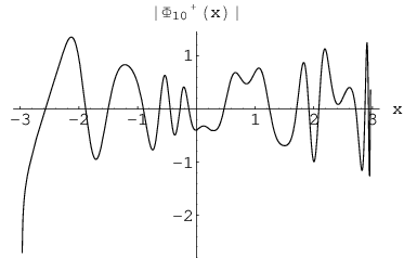
The presumptive Hilbert-Polya operator would have eigenvalues equal to the ’s. It might be of interest to attempt to estimate its eigenfunctions within the same postulated quasi-classical (CBC) framework employed in the CM model, and in our analyses above. In Sec. 6.3 of Junker 1996 (also (Inomata and Junker 1994, eq. (56))) there are presented formulas for the quasi-classical wave functions. The appropriate fractal extensions of these formulas — following the ansatz employed in (5) — would need to be employed (cf. Wójcik et al. 2000). An initial effort of ours along these lines — by simple way of a single illustration — yielded Fig. 18.
In the context of their foundational article (Wu and Sprung 1993, p. 2597) (cf. Tomiya and Sakamoto 2003), “Riemann zeros and a fractal potential”, Wu and Sprung noted that “All the wave functions decay exponentially beyond the turning point, and thus quickly die away. This implies that the lower energy levels have very small influence on the potential beyong their turning points …Clearly, the potential in the low energy range has greater ’responsibility’ than that in a higher energy range, thus it has more structure …Based on this argument, the finest structure will be determined by the wave number of the last wave function.”
It would be of interest to estimate all the wavefunctions in our various analyses above, and examine whether or not the fractal SUSY Schrödinger equation (6) is (at least, approximately) satisfied. This would be, in some sense, a test of the appropriateness of the fractal extension of the CBC relations postulated by Castro and Mahecha (adopted by them in order to avoid having to directly solve (6)). (It would also, of course, be of interest to attempt to solve (6) more directly, rather than having to resort to the fractal CBC ansatz of CM.)
In Fig. 19 we show the counterpart to Fig. 18 based simply on the smooth Wu-Sprung potential, without any fractal contribution, and original (non-fractal) formulas ((Junker 1996, eq. (6.40)), (Inomata and Junker 1994, eq. (56))) for the quasi-classical eigenfunctions. It would be an interesting exercise to further duplicate some of the analyses conducted here, but with the replacement of the fractal CBC equations (5) with the (conventional) CBC equations.

Throughout the minimization analyses above, for the sake of simplicity (and to avoid the possible confusion of issues), we have relied upon a quite elementary least-squares fitting. Modifying this approach to give more equable weighting to the two sets of coupled equations, and perhaps to lower and higher Riemann zeros and turning points might prove useful.
CM believed “that their fractal SUSY QM model, once the optimum value for the amplitude factor is known, has a great chance of truly reproducing the zeta zeros, and proving the [Riemann Hypothesis], by simply establishing a one-to-one correspondence among the values of the infinite phases of our Weierstrass function with the zeta zeros” (Castro and Mahecha 2004, sec. 6). We have tried to make a contribution in such a direction here.
Castro suggested that the most salient/interesting aspect of our several analyses above had emerged in Sec. V.2.1, where for the case we had set the ten phases to zero (doing so which had been strongly suggested by the results of the immediately preceding analysis in which the phases were not constrained, and allowed to vary between 0 and , but found, nevertheless, to be predominantly 0 or ). The estimates of the frequency parameter and the scaling parameter were quite intriguingly close (1.25274 and 1.23289). However, the figure of merit, 7.2358, in this zero-phase analysis was somewhat inferior to that [2.86609] in that unconstrained analysis, which rather induced us here not to subsequently pursue solely further analyses () in which the phases had been a priori set to zero — but rather let them freely vary. Also, we suspected, as previously mentioned, that the predominance of 0’s or ’s might be, in some way, a computational artifact, since these are the imposed limits on the phases. (The minimization procedure, we speculated, might drive the phases to these end points, beyond which it could not further proceed to seek improvements, and would therefore terminate there. Castro suggested that setting the range of possible phases to be would obviate this particular problem — but possibly introduce new ones. We intend to investigate such a direction.)
Perhaps somewhat relatedly, as one of their “spectral speculations”, Berry and Keating (Berry and Keating 1999, p. 260) remarked that the “Maslov phases associated with the [classical periodic orbits of the Riemann dynamics] are also peculiar: they are all . The result appears paradoxical in view of the relations between these phases and the winding numbers of the stable and unstable manifolds associated with periodic orbits , but finds an explanation in a scheme of Connes”. (The Maslov phases appear when one modifies the Bohr-Sommerfield quantization rules by equating the WKB integrals (orbits) to plus a Maslov phase factor, instead of .)
Castro suggested that the possibility the Weierstrass fractal function might assume the form of classical Brownian motion was an unappealing one, seeing that this would apparently imply that the phases () must be random. (In Sec. V.5.1 we deduced certain statistical evidence that the estimated phases [allowed to freely vary] were not, in fact, random. Of course, we know this to be strictly true, since the phases are constructed by our estimation procedure.)
Appendix
At our suggestion, D. Dominici investigated
the problem of inverting the
Wu-Sprung potential (1) (Wu and Sprung 1993, eq. (7)).
His analyses have
been presented in a “preliminary report” Dominici.
Dominici
gives explicitly
the first ten coefficients () of a power series expansion,
| (15) |
where
| (16) |
(For the critical value , above which is single-valued, the expansion (15) is no longer valid. A separate analysis (Dominici, Sec. 2.2) is, then, of interest.) Using just the first three of these coefficients,
| (17) |
we obtain Fig. 20.

In the analyses reported in the body of this paper, we had relied upon the Interpolation command of Mathematica for the purpose of inversion, but we anticipate employing the results of Dominici Dominici in our further work. C. Krattenthaler has indicated that for the purpose of studying the asymptotic behavior of the coefficients of the power series, it would be best to employ the methodology of Lagrange inversion.
Acknowledgements.
Carlos Castro kindly introduced me to his joint work Castro and Mahecha 2004 with Jorge Mahecha, proposed avenues of research to pursue, and discussed in great detail the analytical developments. Further, I would like to express gratitude to the Kavli Institute for Theoretical Physics (KITP) for computational support, to Michael Trott of Wolfram Research Inc. for his more than generous assistance and expertise in terms of Mathematica computations, as well as for his critical interest and comments, and to Diego Dominici for his interest in the problem of inverting the Wu-Sprung potential Dominici.References
- Conrey (2003) J. B. Conrey, Notices Amer. Math. Soc. 50, 341 (2003).
- Bunimovich and Dettmann (2005) L. A. Bunimovich and C. P. Dettmann, Phys. Rev. Lett. 94, 100201 (2005).
- Rockmore (2005) D. Rockmore, Stalking the Riemann Hypothesis (Pantheon, New York, 2005).
- Castro and Mahecha (2004) C. Castro and J. Mahecha, Int. J. Geom. Meth. Mod. Phys. 1, 751 (2004).
- Wu and Sprung (1993) H. Wu and W. L. Sprung, Phys. Rev. E 48, 2595 (1993).
- Berry and Lewis (1980) M. V. Berry and Z. V. Lewis, Proc. Roy. Soc. London 370, 459 (1980).
- Khuri (2002) N. N. Khuri, Math. Phys. Anal. Geom. 5, 1 (2002).
- Rosu (2003) H. C. Rosu, Mod. Phys. Lett. A 18, 1205 (2003).
- van Zyl and Hutchinson (2003) B. P. van Zyl and D. A. W. Hutchinson, Phys. Rev. E 67, 066211 (2003).
- Laskin (2002) N. Laskin, Phys. Rev. E 66, 056108 (2002).
- Inomata and Junker (1994) A. Inomata and G. Junker, Phys. Rev. A 50, 3638 (1994).
- Edwards (1974) H. M. Edwards, Riemann’s zeta function (Academic Press, New York, 1974).
- Ma and Hori (2003) C. Ma and Y. Hori, in ASME 2003 Design Engineering Technical Conferences (2003), (DET2003VIB-48736).
- (14) D. Dominici, eprint math.CA/0510341.
- Bhaduri et al. (2005) R. K. Bhaduri, J. Sakhr, D. W. L. Sprung, R. Dutt, and A. Suzuki, J. Phys. A 38, L183 (2005).
- Planat and Rosu (2003) M. Planat and H. C. Rosu, Phys. Lett. A 315, 1 (2003).
- Rüschendorf (1995) L. Rüschendorf, Ann. Statist. 23, 1160 (1995).
- Katz and Sarnak (1999) N. M. Katz and P. Sarnak, Bull. Amer. Math. Soc. 36, 1 (1999).
- Wu et al. (1990) H. Wu, M. Valliéres, D. H. Feng, and D. W. L. Sprung, Phys. Rev. A 42, 1027 (1990).
- Robnik et al. (1999) M. Robnik, L. Salasnich, and M. Vraničar, Nonlin. Phen. Complex Syst. 2, 49 (1999).
- Finch (2003) S. R. Finch, Mathematical Constants (Cambridge U. P., Cambridge, 2003).
- Apéry (1979) R. Apéry, Astérique 61, 11 (1979).
- Szulga and Molz (2001) J. Szulga and F. Molz, J. Statist. Phys. 104, 1317 (2001).
- Szulga (2002) J. Szulga, Statist. Prob. Lett. 56, 301 (2002).
- Pipiras and Taqqu (2000) V. Pipiras and M. S. Taqqu, Fractals 8, 369 (2000).
- Rawlings (2003) P. K. Rawlings, J. Statist. Phys. 111, 769 (2003).
- Biane et al. (2001) P. Biane, J. Pitman, and M. Yor, Bull. Amer. Math. Soc. 38, 435 (2001).
- Russell and Levitin (1995) G. S. Russell and D. J. Levitin, Commun. Statist.: Simul. Comput. 24, 879 (1995).
- Junker (1996) G. Junker, Supersymmetric Methods in Quantum and Statistical Physics (Springer-Verlag, Berlin, 1996).
- Wójcik et al. (2000) D. Wójcik, I. Białynicki, and K. Życzkowski, Phys. Rev. Lett. 85, 5022 (2000).
- Tomiya and Sakamoto (2003) M. Tomiya and S. Sakamoto, e-J. Surf. Sci. Nanotech. 1, 175 (2003).
- Berry and Keating (1999) M. V. Berry and J. P. Keating, SIAM Review 41, 236 (1999).