Minimal monomial ideals and linear resolutions
Jeffry Phan
Columbia University
Abstract
A minimal monomial ideal is the combinatorially simplest monomial ideal whose lcm-lattice equals a given finite atomic lattice . The minimal ideal inherits many nice properties of any ideal whose lcm-lattice also equals , e.g. Cohen-Macaulayness and the dual property of having a linear resolution. Conversely, any ideal having a linear resolution is shown to be, essentially, minimal.
1 Introduction
We introduce and study minimal monomial ideals; these are the simplest ideals whose lcm-lattice equals a given finite atomic lattice . Recall that if is a monomial ideal minimally generated by , the lcm-lattice of is the set of all least common multiples of the , partially ordered by divisibility. is a finite atomic lattice; Gasharov, Peeva, and Welker proved computes the Betti numbers of (and more, see [12]). They also showed that if , then and have equivalent resolutions up to a relabeling process they make precise (see also the relabeling used in the deformation of exponents of [7] and [15]). Our construction shows every finite atomic lattice is the lcm-lattice of some monomial ideal.
Although the minimal free resolution of a monomial ideal is easily computed, it is unknown how to theoretically describe the maps between the free modules. When has a linear resolution, Reiner and Welker constructed these maps in [11]. Bayer, Peeva, and Sturmfels showed the maps can be thought of as the boundary maps of a simplicial complex when is a generic monomial ideal ([7]) and this idea has been studied in several papers ([4], [15], [13]). It is natural to ask if can be used to describe the maps in the minimal resolution. This question is still widely open, but minimal monomial ideals are one possible avenue of attack: if one can construct the maps for minimal ideals, then up to relabeling the problem is solved for all monomial ideals.
In Section 2 we construct minimal squarefree ideals and prove they are universal in the sense of Theorem 2.8. One corollary is that every simplicial complex is the Scarf complex of some squarefree monomial ideal ([7],[4]). If is acyclic, then supports the minimal resolution of that ideal.
The subset of meet-irreducible elements of plays an essential role throughout this paper. In Section 3, we study how is related to the distributive lattice generated by . Closely related to minimal ideals are the the Hibi ring of and the ideals studied in the series of papers by Herzog, Hibi, and Zheng ([16],[17],[18],[14]); exploration of the connections are left for a future paper.
In Section 4, we study nonsquarefree minimal ideals. As a corollary, we are able to prove the width of bounds the projective dimension of .
In Section 5, we show that many nice properties of pass to the minimal ideal constructed from . In particular, if has a linear resolution, then so does the minimal ideal. We characterize those for which this is possible; a very similar result (by a theorem of Eagon and Reiner) was proved by Yuzvinsky in the setting of rings of sheaves on posets ([5]). Finally, we show that ideals with linear resolutions are minimal up to a common divisor of the generators.
2 Squarefree Constructions
Let be a finite atomic lattice with proper part and let be the subposet of meet-irreducible elements of . Fix a field . We will construct the simplest possible squarefree monomial ideal whose lcm-lattice equals .
For denote by and the order ideal and the order filter generated by . Define where the product is over all . Partially order monomials by divisibility.
Every equals the meet of those satisfying . This implies in if and only if if and only if . Therefore
| (1) |
Theorem 2.1
Let be the atoms of . Define the squarefree monomial ideal by
Then .
Proof Set . Let and let be the support of . Then equals the union of the , , and therefore . It follows that for all . This means the map , , preserves joins and is surjective. is determined by supports and so also preserves meets. is injective because implies , by Equation 1. Therefore is a lattice isomorphism.
Example 2.2
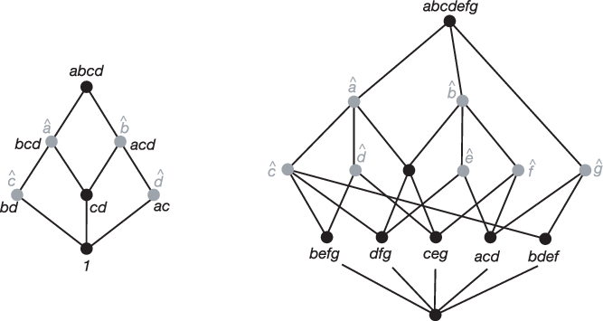
The two examples in Figure 1 illustrate Theorem 2.1. Each has been colored light grey and labeled with the variable instead of . The hats are meant to suggest that every element in is missing the variable . The lefthand figure is the the lcm-lattice of the ideal . The righthand figure is the lcm-lattice of ; in this example the labels of non-atoms have been omitted for clarity.
Example 2.3
Let be the boundary complex of the convex polytope and let be set of faces of ordered by inclusion. The atoms of are the vertices of and the coatoms of are the facets of . Because is coatomic, is the product of those variables corresponding to facets not containing the vertex . Hence is the Cox irrelevant ideal of the toric variety defined by ([8]).
Example 2.4
When is a geometric lattice, coincides with the ideal constructed by Irena Peeva in [1]. In that paper, Peeva proved the minimal free resolution of can be explicitly described using either broken-circuit complexes or Orlik-Solomon complexes. Isabella Novik proved the same can be done using rooted complexes ([9]).
Recall the Taylor complex of is the simplex on with each face labeled by the degree . The Scarf complex is the subcomplex of faces that have unique degree. Assume is not a simplex. The face poset of is then naturally a subposet of and therefore ideals with isomorphic lcm-lattices must have isomorphic Scarf complexes. supports a minimal resolution of if and only if each Betti degree of is the degree of some face of if and only if for all either the closed interval is boolean or the open interval is acyclic. The last equivalence follows from the next theorem, which appears as Theorem 2.1 in [12]; we call a multidegree for which a Betti degree of . Note that we identify the interval topologically with its order complex.
Theorem 2.5
([12]) For and we have , where is the th Betti number in multidegree .
Proposition 2.6
Every simplicial complex not equal to the boundary of a simplex is the Scarf complex of some squarefree monomial ideal. If is acyclic, then supports the minimal resolution of that ideal.
Proof If is a simplex, then is the Scarf complex of the irrelevant ideal and supports the minimal resolution of that ideal. Let be the face poset of . We can assume that is not a simplex or, equivalently, that is atomic. Let be as in Theorem 2.1, so that . It’s easy to see is the Scarf complex of . is the least common multiple of all the generators. is not a betti degree if and only if is acyclic if and only if is acyclic; in this case, the betti degrees are concentrated in so supports the minimal resolution of by Lemma 3.1 in [7].
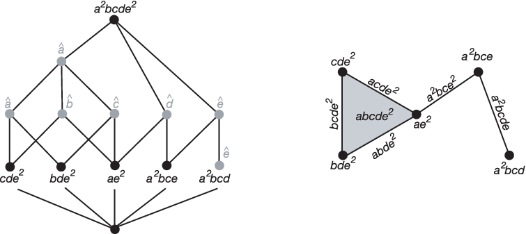
Proposition 2.6 is illustrated in Figure 2. The ideal has been depolarized as in Theorem 4.1; in other words, the polarization , of the given ideal yields .
Definition 2.7
Squarefree minimal ideals are monomial ideals of the form for a finite atomic lattice . Say a monomial ideal is a minimal ideal iff its polarization is a squarefree minimal ideal.
The name is justified by Theorem 2.8, but note that is minimal with respect to generators, not with respect to containment.
Theorem 2.8
Let be any squarefree monomial ideal with and let be the squarefree minimal ideal.
- (i)
.
- (ii)
There exists a -algebra injection sending variables to variables that satisfies . If , then is an isomorphism.
- (iii)
Embed and by identifying a monomial with its support. Then there exists a join-preserving injection such that .
We need some definitions before giving the proof. If and is the unique element covering , then call an essential pair of . Let be as in the theorem and for let be the monomial corresponding to . A variable is said to separate the essential pair if divides but does not divide . Every essential pair is separated by some variable, but not conversely.
Define for each variable the order filter . is the inverse image of under the characteristic map determined by . This map preserves joins so is a filter and its complementary order ideal is join-closed. For define and analagously. If , then doesn’t divide if and only if . Therefore equals the principal order ideal generated by .
If for some , then the lcm-lattice cannot distinguish between and . In this sense, one of the variables is unnecessary.
Lemma 2.9
Let be an essential pair of . Define . Then is not empty, and if and only if separates .
Suppose separates no essential pair. Define . Then .
Proof Note that separates , so implies separates , too. Conversely, suppose separates . is join-closed so it has a maximum element and . Evidently . If they are not equal, there must exist . Then implies implies , a contradiction because is join-closed. Hence and this is equivalent to . is not empty because , , is injective.
For the second statement, assume separates no essential pair. By the preceding argument, if , then this containment is proper. Let be the maximum element of and let . Our task is to find such that , for then . But . Equation 1 implies there exists and we are done.
Proof of Theorem 2.8 To prove it suffices to show each separates at most one essential pair. If and , then by Lemma 2.9 and follows.
For each , choose . Define a -algebra morphism by . Let be an atom and let and be the corresponding generators of and , respectively. Lemma 2.9 implies divides , so . This proves .
For each that separates no essential pair, choose a cover such that . The map will depend on the collection of covers . Fix . For define . Observe that for all , including .
For simplicity regard as the set of subsets of . Define on singletons by . If , then and are incomparable because . Extend by for each . If , then is not contained in the support of for any . This implies is injective.
To see it suffices to prove for all atoms . Recall . Let . Evidently . If , then so that . Therefore and thus . Let . We can assume separates no variable. Because is a cover there exists such that . Then which implies .
For any squarefree ideal , let be the simplicial complex on whose Stanley-Reisner ideal equals .
Corollary 2.10
With the identification in Theorem 2.8 (ii), is a subcomplex of .
In Section 5 we will show that inherits many nice properties of , even though they are generally not homotopy equivalent.
Note that where is generated by binomials . If is a minimal free -resolution of , then is a minimal free resolution of . This is an example of the relabeling process in [12].
We can take this in another direction. Replacing with in the construction in Theorem 2.1 yields a nonminimal ideal whose LCM-lattice equals . For example, if is the boolean lattice with three atoms and coatoms , then . This ideal is natural in a different sense: For any atomic lattice on atoms, a (nonminimal) resolution of can be obtained as a quotient of . To see this, let be the atoms of . Define the map by
is a join-preserving surjection. For the fiber is join-closed and therefore has a maximum element.
Theorem 2.11
Let be a finite atomic lattice on atoms . Let be the minimal free -resolution of . Let be the ideal defined by
Then and . Furthermore is a (generally nonminimal) free resolution of .
Proof Let be a proper subset of and let be the corresponding variable. is not a zero divisor on the quotient of a polynomial ring by a monomial ideal, so induction on the number of generators of shows is exact. Fix and let . Let be different than . It suffices to show have the same image in . The quotient of the monomials is . Let . Need to see . But because and preserves order. is not contained in (else ) and is nonempty, so .
3 The Distributive Completion of
Recall a finite lattice is a distributive lattice if for all
Let be a finite poset and let be the set of all order filters in ordered by reverse inclusion. is a distributive lattice and the order dual version of Birkhoff’s theorem states that every distributive lattice is of this form: if is the set of meet-irreducible elements of , then . See Theorem 3.4.1 in [3]; note that our definition of is dual to the standard one.
Write for the set of subsets of ordered by inclusion. Let be the map . The support of is complementary to the support of the monomial used in Theorem 2.1. is injective by Equation 1 and sends joins to meets.
Theorem 3.1
Let be the surjective map . is order reversing. is isomorphic as a join semilattice to its image under the composition .
Proof is order reversing because is ordered by reverse inclusion. Let be the restriction of to . Then is injective by the discussion preceding Equation 1 and it preserves joins because . Since is also order reversing, and are isomorphic as join semi-lattices.
We call the distributive completion of . The name is justified because any distributive lattice containing as a meet irreducible elements must contain . Hence must contain as a join subsemilattice. The theorem also places a restriction on which posets can be isomorphic to .
Example 3.2
Using Theorem 3.1, one can show the poset in Figure 3 cannot be isomorphic to for any atomic lattice . On the other hand, if , then contains as a subposet. See [19] for properties of posets not containing , which are called series-parallel posets, and their applications in scheduling theory.

Let be as in Theorem 3.1. Each fiber contains a maximum and minimum. Elements of are the maximums of their individual fibers; associated primes of are the minimums of their individual fibers. Furthermore, if we let be the subset of elements such that the prime ideal contains , then is an order ideal of . It will be useful to have another characterization of the primes containing .
Proposition 3.3
Let be a squarefree monomial ideal with . The prime contains if and only if
| (2) |
If this is true, then is an associated prime if and only if the union is irredundant if and only if the intersection is irredundant.
Proof The two conditions in Equation 2 are easily seen to be equivalent. if and only if is a face of where . is a face of if and only if atoms such that . This is true if and only if because the union is an order filter. Moreover, this union is irredundant if and only if is a facet of .
Example 3.4
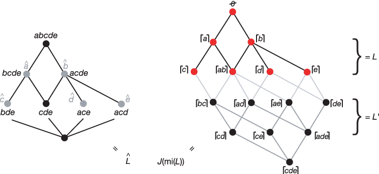
In Figure 4, each element of is labeled by the minimal generators of the corresponding order filter. The image of has been highlighted. Let be the complement of in . Note the six associated primes of appear in under this labeling, as do the two unassociated primes and . is not homotopy equivalent to , but it is homotopy equivalent to the subcomplex of supported on the vertices , which minimally generate the filter .
Furthermore, is a coatomic lattice in this case, and therefore it’s order dual is a finite atomic lattice. This is not true in general. It would be interesting to characterize those atomic lattices for which the order dual of is also an atomic lattice.
4 Nonsquarefree Ideals and Depolarization
One consequence of Theorem 2.5 is that the length of the minimal resolution of is to the rank (or height) of . In this section we will characterize which monomial ideals have polarizations that are minimal ideals. As a corollary we will prove that the width of also bounds the projective dimension of (Theorem 4.4).
We first recall some facts about the polarization operation. If is a monomial ideal, define a simple polarization of to be the monomial ideal obtained as follows. If is the highest power of appearing in any generator , then introduce a new variable and let be the ideal obtained by replacing by in each generator divisible by . A polarization of is a squarefree ideal obtained by iterated simple depolarizations. If where is a polynomial ring containing , then is the quotient of by an ideal generated by a regular sequence consisting of binomial differences of variables. Thus many nice properties hold for if and only if they hold for . See, for example, [6] for details on polarization.
Proposition 4.1
Let be a finite atomic lattice and let be the minimal ideal. Let be a partitioning of into chains. For each choose . Define the ideal to be
Then is a polynomial ring, is a monomial ideal, and .
Proof Evidently is combinatorially equivalent to . It’s easy to see for any monomial ideal .
Corollary 4.2
Let and let . Then if and only if and are comparable.
Proof If and are comparable, then by the proposition since we can take and let be singletons for . Suppose and are incomparable and let and be essential pairs. For all denote by the image of in . If , then divides but divides neither nor and therefore . This implies . If , then appears with exponent 1 in and and polarizing cannot distinguish between and ; therefore
Corollary 4.3
If is coatomic, then there is no monomial ideal on fewer than variables that has lcm-lattice equal to .
Proof If such an ideal existed, then a minimal one exists so we can assume . is coatomic iff is an antichain, so there would be no way to depolarize to obtain .
Recall the width of a poset is one less than the cardinality of the longest antichain in .
Theorem 4.4
Let be a monomial ideal with . Then
Proof by Theorem 2.5. Dilworth’s theorem asserts that any poset can be partitioned into chains. Proposition 4.1 implies there exists a monomial ideal in variables whose lcm-lattice equals . Theorem 2.5 implies and have resolutions of the same length and Hilbert’s Syzygy theorem implies .
Suppose now that is a squarefree ideal and let be the Stanley-Reisner ideal of the simplicial complex on that is Alexander dual to . Terai was the first to prove the connection between the projective dimension of and the Castenuovo-Mumford regularity of . See also [20].
Theorem 4.5
(Terai [10]) Let be a squarefree ideal and let be the Alexander dual ideal. Then
The next corollary is a natural consequence. Since we know there exists a simplicial complex on at most vertices that has intersection lattice equal to , we also get an easy upper bound on the nonvanishing homology of .
Corollary 4.6
Let and be as above.
- (i)
.
- (ii)
if , where denotes the th reduced homology of .
Proof follows immediately from Terai’s theorem and Theorem 4.4. For we can assume each variable divides some generator of ; otherwise SR(I) would be acyclic because its dual would be a cone. is isomorphic to the intersection lattice of by Proposition 2.3 in [12] (see also [5]). Therefore the order complex of is homotopy equivalent to . The last two sentences are true if is replaced by , so follows from Alexander duality.
5 Inherited Properties
Henceforth will be a monomial ideal such that . In this section we prove that the minimal ideal inherits many nice properties of . For example, if has a linear resolution, then so does . As a corollary, we prove that ideals with linear resolutions are minimal up to a common factor dividing all the generators. Theorem 5.8 characterizes those atomic lattices for which has a linear resolution. A very similar (by Eagon-Reiner) formulation was proved by Yuzvinsky ([5], Theorem 6.4) in the broader setting of rings of sections of sheaves over .
Recall that is said to have linear quotients if there is an ordering, say the given one, such that is generated by variables for each . If is squarefree, then has linear quotients if and only if is shellable ([18], Theorem 1.4). If is squarefree, say is matroidal if is a matroid. is matroidal if and only if for all and all dividing , there exists that divides .
Proposition 5.1
Let be a monomial ideal with .
- (i)
. If is pure, then so is .
- (ii)
is Cohen-Macaulay if and only if and is Cohen-Macaulay.
- (iii)
Suppose is squarefree. If has linear quotients then has linear quotients. If is matroidal, then so is .
- (iv)
.
Proof Polarizing, if necessary, we can assume is squarefree. Then each associated prime of determines an associated prime of of the same codimension, by Proposition 3.3. This proves . follows from and the fact that and have minimal resolutions of the same length ([12], Theorem 3.3). is immediate from the preceding definitions.
To prove , embed in as in Theorem 2.8. The generators of are obtained from the generators of through multiplication by new variables. By induction it suffices to prove the assertion when there is a single new variable . Set and let be an th betti degree with . Then or , so .
For the rest of the section we will focus on linear resolutions. Passing to the minimal ideal usually does not commute with Alexander duality, so the next theorem is independent of the previous proposition.
Theorem 5.2
Let be a monomial ideal with . If has a linear resolution, then so does .
We postpone the proof. Lemma 5.3 will be essential for what follows. Hartshorne proved that every Cohen-Macaulay variety is connected in codimension 1 (see [2], Theorem 18.12). Lemma 5.3 asserts that more is true if we limit ourselves to simplicial complexes, which are essentially unions of coordinate planes.
Lemma 5.3
Let be a simplicial complex on . Let be the subcomplex generated by faces which are the intersections of the facets of containing . Assume is not a simplex. If is Cohen-Macaulay, then is Cohen-Macaulay and of codimension 1 in .
Proof if and only if is a simplex. Assume is CM but not a simplex. If or 1, then the assertion is easily verified. By induction, we can assume is CM implies is CM of codimension 1 if . Let . The Eagon-Reiner theorem along with Theorem 2.5 implies is pure of codimension 1. To see this, let be the Stanley-Reisner ideal of the Alexander dual . covers an atom if and only if is the betti degree of a first syzygy because has a linear resolution. Call an element that covers an atom a super atom. The complement of , an atom, is a facet of . The complement of , a super atom, is a facet of . Therefore is pure and of codimension 1.
Let . Our task is to show has at most top dimensional homology. If , then . Since is CM, the induction hypothesis implies is CM of codimension 1 in ; in particular, it has at most top dimensional homology. But , so we are done if .
It remains to prove has no homology in dimension . is obtained from by attaching -simplices along codimension 1 faces. Say is fully attached if . If is fully attached, then attaching adds only a -cell and cannot affect homology in dimension . If is not fully attached, then is homeomorphic to a -disk. Simplicially collapse along one of its free faces; the remaining complex deformation retracts to . Therefore if is not fully attached, attaching it to cannot affect homology in any dimension. We’ve shown that if . This concludes the proof.
Corollary 5.4
Let be the ideal generated by the betti degrees of the first syzygies of . If has a linear resolution, then so does .
Proof We can assume is squarefree. Then . The assertion now follows from Eagon-Reiner and Lemma 5.3.
We state the next lemma for easy reference; it is an immediate consequence of Theorem 2.5.
Lemma 5.5
Let be a squarefree monomial ideal such that . If and , then . Moreover, if has a linear resolution then so does .
The betti degrees generally do not form an order ideal in , not even when has a linear resolution. Also, the projective dimension of can be much smaller than the length of so it is somewhat surprising that we can prove statements about all of when the resolution of is nicely behaved.
Proposition 5.6
Let be a monomial ideal with . Suppose has a linear resolution.
- (i)
is a graded lattice.
- (ii)
Let . If covers , then .
- (iii)
If is an th betti degree of , then .
- (iv)
Let . Suppose is squarefree and every divides some generator of . Then where is the face complementary to . In particular, .
Proof : With the notation of Corollary 5.4, also has a linear resolution. By induction on we can assume is graded, since . Any maximal chain of intersects in a maximal chain. It follows that is graded and .
: By Lemma 5.3 and induction it suffices to prove the statement when is an atom. In this case, is a super atom so that is a second betti degree of and therefore because has a linear resolution.
: This follows from and Theorem 2.5.
: By Lemma 5.5, it suffices to prove the statement when . By induction, we can assume where . From the proof of , .
Say a monomial ideal is uniformly generated if its generators all have the same degree. We need one more result before proving Theorem 5.2
Proposition 5.7
Let be a monomial ideal with . If has a linear resolution, then is uniformly generated. Moreover, if and covers , then .
Proof We will prove the second statement first. Let be the product of all such that . Set . Then so using Lemma 5.3 we can repeatedly replace with , if necessary, and assume is an atom. Evidently . Because has a linear resolution, . Identify with as a subring of as in Theorem 2.8. For every atom , for some monomial . This implies and the second claim follows.
In the presence of the second assertion, is uniformly generated if and only if is graded. The first assertion now follows from Proposition 5.6.
Proof of Theorem 5.2 After polarizing, we can assume is squarefree. Modding out by extra variables, we can assume every divides some generator of . By Eagon-Reiner, it suffices to show is CM. Let . We can assume is a face in the intersection lattice, for if not, then is a cone. We need to prove has at most top dimensional homology. By Lemma 5.5 we can assume so that . Proposition 5.6 implies . Because and are both homotopy equivalent to and because is CM, it suffices to prove .
Let . We can assume by induction on the dimension. If , then so that is minimal. Then .
Now assume . Then . Proposition 5.7 implies and are uniformly generated, say by generators of degree and , respectively. Hence the generators of all have degree . Then . As above, this implies and the proof is complete.
We close this section with a characterization of which finite atomic lattices support a linear resolution. Yuzvinsky proved a similar statement in the setting of rings of sections of sheaves on poets (Theorem 6.4, [5]). As a corollary, we prove that any monomial ideal that has a linear resolution is essentially minimal.
Theorem 5.8
Let be a finite atomic lattice. The minimal ideal has a linear resolution if and only if
- (i)
is Cohen-Macaulay as a poset and
- (ii)
if and covers , then .
Proof Suppose and hold. In the presence of , is uniformly generated if and only if is graded. Let be the degree of the generators of . Then implies . Because is CM, Theorem 2.5 implies the can only be nonzero if , or equivalently . This implies , and thus , has a linear resolution.
Conversely, suppose has a linear resolution. Statement follows from Proposition 5.6. Let . Now consider as the intersection lattice of . To keep the argument uniform we will work with the polar face poset , which naturally contains as a subposet. Let . We need to show the order complex of has at most top dimensional homology. By Lemma 5.5 we can assume . If , then is homotopy equivalent and of equal dimension to . Since is CM, has at most top dimensional homology. If , then repeatedly replacing by if necessary, we can assume is an atom of , i.e. a facet of .
Proposition 5.6 implies . Let be the super atoms covering . Then
where is the LCM-lattice of . Let be the intersection of the . The proper part of any poset is homotopy equivalent to the proper part of the join closure of its atoms, so is homotopy equivalent to .
Eagon-Reiner imply is CM. Let be the codimension 1 subcomplex of along which is attached. The facets of are . Evidently equals the proper part of . If is fully attached, then is a sphere of dimension . If is not fully attached, then is a codimension 1 disk, and hence is contractible. In any case, has no homology in dimension . Since is also homotopy equivalent to , the proof is complete.
We can now show that monomial ideals that have linear resolutions are essentially minimal ideals.
Corollary 5.9
Let be a squarefree monomial ideal. Assume that and that has a linear resolution. If , then .
Proof Embed in as in Theorem 2.8. Suppose for some that doesn’t separate an essential pair. Let be a maximal element not in and suppose covers . By Lemma 5.7, . Multiplying the relevant generators by increases the degree of but not the degree of . Hence , contradicting Propostion 5.6. This implies if doesn’t separate an essential pair.
Since , every must separate an essential pair. An argument similar to the one above shows no two can separate the same essential pair, i.e. for all . Modding out by extra variables we can assume every divides some generator of . Hence . This implies that is an isomorphism of lattices, and the claim follows.
Acknowledgements. The author thanks Dave Bayer for many helpful discussions and suggestions.
References
- [1] I. Peeva. Resolutions and lattices. Homology Homotopy Appl., 4:427–437, 2002.
- [2] David Eisenbud. Commutative Algebra, volume Graduate Texts in Mathematics, 150. Springer-Verlag, 1995.
- [3] R.P. Stanley. Enumerative Combinatorics. Cambridge University Press, 1997.
- [4] D. Bayer and B. Sturmfels. Cellular resolutions. J. Reine angew. Math., 502:123–240, 1998.
- [5] Sergey Yuzvinsky. Cohen-macaulay rings of sections. Adv. in Math., 63(2):172–195, 1987.
- [6] Sara Faridi. Monomial ideals via squarefree ideals. arXiv:math.AC/0507238, 2005.
- [7] D. Bayer, I. Peeva and B. Sturmfels. Monomial resolutions. Math. Res. Lett., 5:31–46, 1998.
- [8] D. Cox. The homogeneous coordinate ring of a toric variety. J. Algebraic Geom., 4(1):17–50, 1995.
- [9] Isabella Novik. Lyubeznik’s resolution and rooted complexes. J. Algebraic Combin., 16(1):97–101, 2002.
- [10] N. Terai. Alexander duality theorem and stanley-reisner rings. RIMS Kokyuroku, 1078:174–184, 1999.
- [11] V. Reiner and V. Welker. Linear syzygies of stanley-reisner ideals. Math. Scand., 89:117–132, 2001.
- [12] V. Gasharov, I. Peeva, and W. Welker. The lcm-lattice in monomial resolutions. Math. Res. Lett., 6:521–522, 1999.
- [13] E. Batzies and V. Welker. Discrete morse theory for cellular resolutions. J. Reine Angew. Math., 543:147–168, 2002.
- [14] J. Herzog, T. Hibi, and X. Zheng. The monomial ideal of a finite meet-semilattice. 2003.
- [15] E. Miller, B. Sturmfels, and K. Yanagawa. Generic and cogeneric monomial ideals. J. Symbolic Comput., 29:691–708, 2000.
- [16] J. Herzog and T. Hibi. Level rings arising from meet-distributive meet-semilattices. arXiv:math.AC/0403534, 2004.
- [17] J. Herzog and T. Hibi. Distributive Lattices, Bipartite Graphs and Alexander Duality. arXiv:math.AC/0307235, 2003.
- [18] J. Herzog, T. Hibi, and X. Zheng. Dirac’s theorem on chordal graphs and alexander duality. preprint, 2003.
- [19] I. Rival. ”Stories about order and the letter N (en)” in Contemporary Mathematics: Combinatorics and Ordered Sets, volume 57. 1986.
- [20] Dave Bayer, Hara Charalambous, and Sorin Popescu. Extremal betti numbers and applications to monomial ideals. J. Algebra, 221:497–512, 1999.