Extrinsic versus intrinsic diameter
for Riemannian
filling–discs
and van Kampen diagrams
Abstract
The diameter of a disc filling a loop in the universal covering of a Riemannian manifold may be measured extrinsically using the distance function on the ambient space or intrinsically using the induced length metric on the disc. Correspondingly, the diameter of a van Kampen diagram filling a word that represents the identity in a finitely presented group can either be measured intrinsically in the 1–skeleton of or extrinsically in the Cayley graph of . We construct the first examples of closed manifolds and finitely presented groups for which this choice — intrinsic versus extrinsic — gives rise to qualitatively different min–diameter filling functions.
2000 Mathematics Subject
Classification: 53C23, 20F65, 20F10
Key words and phrases: diameter,
isodiametric inequality, van Kampen diagram
1 Introduction and preliminaries
A continuous map from the unit disc to the universal cover of a Riemannian manifold is called a disc–filling for a loop in when the restriction of to is a monotone reparameterisation of . According to context, one might measure the diameter of such a disc–filling intrinsically using the pseudo–distance on defined as the infimum of the lengths of curves such that is a path from to , or extrinsically using the distance function on the ambient manifold:
These two options give different functionals on the space of rectifiable loops in : the intrinsic and extrinsic diameter functionals , defined by
where, in each case, the supremum ranges over loops in of length at most and the infimum over disc–fillings of .
There is an obvious inequality , which passes to the functionals: for all . One anticipates that for certain compact manifolds , families of minimal intrinsic diameter filling–discs might fold–back on themselves so as to have smaller extrinsic than intrinsic diameter, and the two functionals might then differ asymptotically. However, it has proved hard to animate this intuition with examples. In this paper we overcome this difficulty.
Theorem 1.1
For every , there is a closed connected Riemannian manifold and some such that and .
[For functions we write when there exists such that for all , and we say when and . We extend these relations to accommodate functions with domain by declaring such functions to be constant on the half–open intervals .]
Our main arguments will not be cast in the language of Riemannian manifolds but in terms of combinatorial filling problems for finitely presented groups. There is a close correspondence, given full voice by M. Gromov [7, 8], between the geometry of filling–discs in compact Riemannian manifolds and the complexity of the word problem in . Most famously, the 2–dimensional, genus–0 isoperimetric function of has the same asymptotic behaviour as (i.e. is equivalent to) the Dehn function of any finite presentation of . (See [3] for details.) But the correspondence is wider: most natural ways of bounding the geometry of filling–discs in a manifold correspond to measures of the complexity of the word problem in . The following theorem, proved in Section 2, says that it applies to and , and their group theoretic analogues and (as defined below).
Theorem 1.2
If is a finite presentation of the fundamental group of a closed, connected, Riemannian manifold then
Let be a finite presentation of a group . The length of a word in the free monoid is denoted . Let denote the word metric on associated to . If in (in which case is called null–homotopic) then there exist equalities in the free group of the form
where and . Ranging over all such products freely equal to , define to be the minimum of , and define to be the minimum of
where denotes the element of represented by . Define by letting and be the maxima of and , respectively, over all null–homotopic words with .
As we will explain in Section 2, one can reinterpret and using “combinatorial filling–discs” (van Kampen diagrams) for loops in the Cayley 2–complex of . Then relating the Cayley 2–complex of to will lead to a proof of Theorem 1.2.
In Section 3 we describe an infinite family of finite presentations whose diameter functionals exhibit the range of behaviour described in the following theorem.
Theorem 1.3
For every , there is a group with finite presentation and some such that and .
Theorem 1.1 is an immediate consequence of Theorems 1.2 and 1.3 because, as is well known, every finitely presentable group is the fundamental group of a closed connected Riemannian manifold.
Our results prompt the following questions. What is the optimal upper bound for in terms of for general finite presentations ? How might one construct a finite presentation for which is bounded above by a polynomial function and is bounded below by an exponential function?
1.1 A sketch of the proof of Theorem 1.3
We prove Theorem 1.3 by constructing a novel family of groups . They are obtained by amalgamating auxiliary groups and along an infinite cyclic subgroup generated by a letter .
For each positive integer , one finds an edge–loop in the Cayley 2–complex of that has length roughly and intrinsic diameter roughly . And the reason for this large intrinsic diameter is that in any filling (that is, any van Kampen diagram), there is a family of concentric rings of 2–cells (specifically –rings, as defined in Section 4) that nest to a depth of approximately .
Let us turn our attention to the role of . For each integer there are “shortcut words” of length roughly that equal in . In the Cayley 2–complex of these mitigate the effect of the nested –rings and cause our large intrinsic–diameter diagrams to have smaller extrinsic diameter. This is illustrated in the leftmost diagram of Figure 1.
However there remains a significant problem. In the Cayley 2–complex of , the path corresponding to and the path of its shortcut word, together form a loop. This loop can be filled. We call any filling-disc for this loop a shortcut diagram — of the middle diagram of Figure 1 is an illustration. One could insert two back–to-back copies of the shortcut diagram to get a new filling–disc for our original loop, as illustrated in the rightmost diagram of the figure. The danger is that this lowers intrinsic diameter and thereby stymies our efforts to separate the two diameter functionals of . But is built in such a way that the shortcut diagrams are fat — that is, they themselves have large intrinsic diameter (see Section 5.2). So inserting shortcut diagrams decreases intrinsic diameter far less than the presence of shortcut words decreases extrinsic diameter.
We would like to say that the upshot is that for , the intrinsic diameter functional is at least and the extrinsic diameter functional at most . But, in truth, technicalities make our bounds, detailed in Theorem 7.3, more complicated.

A noteworthy aspect of the construction of is the use of an asymmetric HNN extension (cf. Section 3.1). We anticipate such extensions will prove useful in other contexts. We build by amalgamating with groups of the form . We build by starting with a finitely generated free group and taking a number of HNN extensions and amalgamated free products. All of these groups have compact classifying spaces; has geometric dimension . The Dehn function of is at most for some constant — see Remark 7.5.
1.2 The organisation of this article
In Section 2 we prove Theorem 1.2, establishing the qualitative agreement of the group theoretic and Riemannian definitions of diameter. In Section 3 we present the groups that will be used to prove Theorem 1.3. Section 4 is a brief discussion of rings and corridors — key tools for analysing van Kampen diagrams. In Sections 5 and 6 we explain the salient isodiametric and distortion properties of and . In Section 7 we prove the main theorem, modulo generalities about the diagrammatic behaviour of retracts and amalgams, which we postpone to Section 8. Section 9 is dedicated to a proof that, up to equivalence, extrinsic and intrinsic diameter are quasi–isometry invariants amongst finitely presentable groups.
2 Riemannian versus combinatorial diameter
In this section we reformulate the combinatorial intrinsic and extrinsic diameter filling functions for finitely presented groups in terms of van Kampen diagrams, and then relate them to their Riemannian analogues.
2.1 Diameter of van Kampen diagrams
Let be a finite presentation of a group . Let be a van Kampen diagram over with base vertex . (We assume that the reader is familiar with basic definitions and properties of van Kampen diagrams and Cayley 2–complexes — [3] is a recent survey.) Let be the path metric on in which every edge has length one and let denote the word metric on associated to . Let be the Cayley graph of with respect to and let be the label–preserving graph–morphism with . Define the intrinsic and extrinsic diameter of by
We shall show that the algebraic definitions of diameter for null–homotopic words given in Section 1 are equivalent to
Given a van Kampen diagram for , one can cut it open along a maximal tree in to produce a “lollipop” diagram (with a map ) whose boundary circuit is labelled by a word that equals in and has for all . There is a natural combinatorial folding map such that .
It follows that , where denotes the element of represented by , is at most , because corresponds to a vertex on . Thus the algebraic version of is bounded above by the geometric version. For the opposite inequality, suppose that is a word of the form where for all , and in . Define . Suppose minimises and is of minimal length amongst all words that minimise . There is an obvious lollipop diagram with boundary word . A van Kampen diagram for with can be obtained from this by successively folding together pairs of edges with common initial point and identical labels. (A concern is that in the course of this folding, 2–spheres might be pinched off, but minimising avoids this.)
, as defined above, differs from of Section 1 by at most . This can be shown by an argument similar to the one above, expect that for the first inequality the tree should be chosen to be a maximal geodesic tree based at , and when proving the reverse inequality one must specify first that minimises and then that it has minimal length subject to this constraint. This discrepancy is of no great consequence for us since it has no effect on the –class of the resulting functional.
We will use the van Kampen–diagram interpretations of and in the remainder of this article.
2.2 Generality
With an eye to future applications and to highlight the essential ingredients of our arguments, in this subsection and the next we will work in a more general setting than that of Riemannian manifolds.
Definition 2.1
Define the intrinsic and extrinsic diameters of a disc–filling in a metric space by
where is the pseudometric
on . Define by
[In closer analogy with the definitions in the previous subsection, one could deal instead with based loops and discs and define diameter functions in terms of distance from the basepoint. This makes little difference: the resulting functions are .]
Lemma 2.2
Let be the universal cover of a compact geodesic space for which there exist such that every loop of length less than admits a disc–filling of intrinsic diameter less than . Equip with the induced length metric. Then and are well–defined functions .
Proof. First observe that every rectifiable loop in admits a disc–filling of finite intrinsic diameter: given a disc–filling of a rectifiable loop one can triangulate the disc so that the image of each edge has diameter at most , and then one can modify away from and the vertex set so that its restriction to each internal edge is a geodesic and every triangle has intrinsic diameter at most .
Next, suppose is a loop in of length . Shrinking if necessary, we may assume that balls of radius in lift to . Cover with a maximal collection of disjoint balls of radius ; let be the set of lifts of their centres. Partition into arcs, each of length at most and with end points . Each is a distance at most from a point , and the distance from to is less than (indices modulo ). The loops made by joining to , then to , then to (each by a geodesic), and then to by an arc of , each have total length at most . So, by hypothesis, they admit disc–fillings with intrinsic diameter at most . Such disc–fillings together form a collar between and a piecewise geodesic loop formed by concatenating at most geodesic segments, each of length at most with endpoints in . Modulo the action of , there are only finitely many such piecewise geodesic loops, and by the argument in the previous paragraph each one admits a filling of finite intrinsic diameter. It follows that and (hence) are well–defined functions.
Remark 2.3
If , the universal cover of a closed connected Riemannian manifold , then it satisfies the conditions of Lemma 2.2. Indeed, the required and exist for any cocompact space that is locally uniquely geodesic, for example a space with upper curvature bound in the sense of A.D. Alexandrov — i.e. a CAT space [5]: by cocompactness, there exists such that geodesics are unique in balls of radius , and any loop in such a ball can be filled by coning it off to the centre of the ball using geodesics.
2.3 The Translation Theorem
Theorem 1.2 is a special case of the following result.
Theorem 2.4
Suppose a group with finite presentation acts properly and cocompactly by isometries on a simply connected geodesic metric space for which there exist such that every loop of length less than admits a disc–filling of intrinsic diameter less than . Then and .
We shall first establish the assertion concerning extrinsic diameter and the relation .
Map the Cayley graph of to as follows: fix a basepoint , choose a geodesic from to its translate for each generator of , and then extend equivariantly. Following [3], a path in is called word–like if it is the image in of an edge–path in the Cayley graph.
Each 2–cell in the Cayley 2–complex is attached to the Cayley graph by an edge–loop labelled by one of the defining relations of . For each we choose a filling disc of finite intrinsic diameter for the corresponding word–like loop in based at . We then map to by the –equivariant map that sends each 2–cell with boundary label to a translate of .
Using a collar between an arbitrary rectifiable loop in and a word–like loop, as in the proof of Lemma 2.2, one can show that there is no change in the classes of either or if one takes the infima in their definitions to be over fillings of word–like loops only. Having made this reduction, the relation becomes obvious, since one gets an upper bound on the intrinsic diameter of discs filling a word–like loop simply by taking the image in of a minimal intrinsic diameter van Kampen diagram for the appropriate word. A technical concern here is that need not be a topological 2–disc, but rather may be a finite planar tree–like arrangement of topological 2–discs and 1–dimensional arcs. This can be overcome by extending to a small regular neighbourhood of by a map that is constant on the slices of the annulus .
The same argument yields , and the converse is an easy approximation argument (the details of which are included in Lemma 2.5). Briefly, noting that the map of the Cayley graph of to is a quasi–isometry, we need only show that a disc–filling of a word–like loop gives rise to a van Kampen diagram for the corresponding word that is –close to . Such an approximating disc is obtained by simply taking a fine triangulation of , and then labelling it as in the proof of Lemma 2.5.
The remainder of this section is devoted to the most difficult relation in Theorem 2.4, namely . Like the argument sketched above, the proof of this assertion involves constructing a suitable combinatorial approximation to a Riemannian filling of a word–like loop. The control required in this approximation is spelt out in the following lemma.
Lemma 2.5
To prove , it suffices to exhibit constants such that, given a filling of intrinsic diameter for a word–like loop , one can construct a combinatorial cellulation of and a map with the following properties:
- (1)
the attaching map of each 2–cell of has combinatorial length at most ,
- (2)
adjacent vertices in are mapped by to points that are a distance at most apart in ,
- (3)
from each vertex of , one can reach by traversing a path consisting of at most edges, and
- (4)
the vertices on are mapped by to points on , and their cyclic ordering is preserved; moreover, every vertex of is in .
Proof. In light of Theorem 9.1, we may take to be a finite presentation well adapted to the geometry of . Thus we fix so that is the –neighbourhood of , and as generators of we take the set of those such that . As relations we take all words of length at most in the letters that equal the identity in . The remainder of our proof shows that these relations suffice; cf. [5, page 135].
Given a word in the generators that equals in , we consider the corresponding word–like loop in . By construction, there are constants such that the length of is at most . So we will be done if, given a disc–filling of with intrinsic diameter , we can exhibit a van Kampen diagram for with intrinsic diameter bounded above by a linear function of .
Let be as described in the statement of the lemma and label each vertex by a group element such that is within of . Label an edge from a vertex to a vertex by , which is in . For vertices of , we choose to be one of the endpoints of the edge of the word–like loop in which (the image of) lies.
By hypothesis, the boundary of each 2–cell in the cellulation is then labelled by a word that belongs to . This process does not quite yield a van Kampen diagram for the original word , but rather for a word that is equal to modulo the cancellation of edge–labels . (Our convention on the choosing of for vertices on ensures this equality.) Collapsing such edges yields the desired diagram.
Continuing the proof that , we concentrate on a disc–filling of intrinsic diameter for a word–like loop with basepoint . We will construct and satisfying the conditions of Lemma 2.5 with , and in three steps.
(i) Constructing the tree of a fine triangulation.
Since is continuous and is compact, admits a finite triangulation such that maps each triangle to a subset of of diameter at most . Fix . Fix an ordering on the vertices of and, proceeding along the list, choose an embedded arc in joining to as follows so that is a tree. Having defined for each , to define first choose an embedded arc from to of length at most , and arrange that it pass through no vertices in (more on this in a moment) and finally replace its terminal segment beginning at the first point it meets in , with the arc in between and . By construction is the set of leaves of . Were it not for the –error terms, the diameter of would be at most . We choose small enough so that the diameter is no more than .
[Technicalities: We introduced to avoid a discussion of the existence of geodesics in the pseudometric space . We can arrange that not pass through by replacing with a map that is constant on a small disc about each and which, on the complement of the union of these disjoint discs, is where is a homeomorphism stretching an annular neighbourhood of each deleted disc to a punctured disc with the same centre. The distances between distinct vertices in and are the same and, in the latter, a path can take a detour near any vertex without adding any length.]
We intend to combine and to give a cellulation with the properties required for Lemma 2.5. However, as things stand, the intersection of with the cells of could be extremely complicated. To cope with this we introduce a hyperbolic device to extract the essential features of the pattern of intersections.
(ii) Taming the intersection of with .
As above, is the set of vertices of that lie in the interior of . We impose a complete hyperbolic metric on in such a way that is a regular geodesic polygon and the 1–cells of are geodesics in the hyperbolic metric. For each let be the unique geodesic in the same homotopy class of ideal paths from to in as . To aid visualisation, we are going to talk of these arcs as being red.
The point of what we have just done is that it vastly simplifies the pattern of intersections of the with : the pattern of intersections of the with a triangle is the simple pattern shown in Figure 2 (except if the triangle has as one of its vertices then some of the red edges can meet , indeed the sides of the triangle may be red). Moreover, the larger–scale geometry has been retained in a way that allows us to construct a cellulation with combinatorial diameter at most a linear function of , as we will explain.

(iii) Constructing the good cellulation and map .
We begin by taking the cellulation consisting of overlaid with . That is, the vertices are the vertices of and the points of intersection of with edges of , and the edges come in two types: black edges which are edges of (which may be partitioned into multiple edges by vertices on ), and red edges, which are arcs in between vertices. Define to be the restriction of to .
We will alter (and ) and the paths until we can control their combinatorial lengths in terms of the lengths of the and thereby get an upper bound on the intrinsic diameter of .
It will be convenient if whenever are distinct, and meet only at . Achieve this by doubling , and joining doubled vertices by a new black edge — see Figure 3. Call the new combinatorial disc and define by letting be where is the image of under the obvious combinatorial retraction of onto .

Repeat the following for each such that has combinatorial length at least 2. As is in the same homotopy class of ideal paths from to of as , the sequence of edges crosses is also crossed by in the same order, except may make additional intersections en route. That is, if are the points of intersection of with numbered in order along with , and all other on so a black edge , then there are points occurring in order along with , and on for all other . For all let be the integer part of the length of the segment of from to . Note that increases monotonically from to , and takes all possible integer values in that range because of the condition that the diameters of the images of the triangles in are at most . For each , collapse to a single vertex the minimal arc of that includes all red vertices such that . Note that as each arc is collapsed the complex remains topologically a disc since the arc does not run between two boundary vertices.
The result is the desired cellulation of and we define by setting to be for any choice of preimage of under the quotient map . All that remains is to explain why and satisfy the conditions of Lemma 2.5 with , , and .
The faces of each have at most six sides since this was the case for (six being realised when red edges cut across each of the corners of a triangle of ) and the subsequent collapses of edges can only decrease the number of sides, which proves (1).
For (2), first suppose and are vertices in joined by a red edge. Then they are images of vertices and on the some path in such that , and . But then, as ,
Next suppose and are vertices in joined by a black edge. Assume they are images of vertices and on paths and in such that and are joined by a black edge. Then and there are and on and such that , , , and . So
The remaining possibility is that and are joined by a black edge but one or both is in and so is not on any in . Similar considerations to the previous case yield .
By construction, for all , the combinatorial length of the images in of is at most the length of , and so at most and we have (3). And finally, (4) is immediate from the way we constructed and .
3 The groups for Theorem 1.3
The groups that we use form a 2–parameter family
where are integers.
3.1 The “Fat–Shortcuts” Groups
We construct by amalgamating , a double HNN–extension of , with two isomorphic copies of , where the action of is chosen so that a certain cyclic subgroup of is distorted in a precisely controlled manner as will be required in Lemma 5.2. The two copies of are amalgamated with along the cyclic subgroups . [The distortion of a finitely generated subgroup of a finitely generated group measures the difference between the word metric on and the restriction to of the word metric of — see [5], page 506.]
We first take a presentation of by choosing a basis for and specifying the action of :
| generators | |
| relations | |
Let be a second copy of with corresponding presentation in which the generators are .
We define to be the amalgam along of the asymmetric HNN extension with the standard HNN extension . [This is obtained from by the Tietze move introducing .] Thus has presentation
Finally, we define
where the amalgamations identify with and , respectively. Thus, writing and , a presentation for is
The asymmetric nature of the quasi–HNN presentation of will be important in Section 5.1 when we wish to force shortcuts to be fat — see Figure 5 for an example and Section 5.4 for the general argument. As we indicated in the introduction, this fatness is the key to forcing the behaviour of the intrinsic and extrinsic diameter functionals to diverge.
3.2 The –rings groups
The groups , whose presentations we give below, are 2–fold HNN extensions of the free–by–free groups . By deleting from the generator and the defining relations in which it appears, one recovers the groups constructed by the first author in [2]; these have isodiametric properties that prevent their asymptotic cones from being simply connected.
We define , where the first generator of acts on as an automorphism with polynomial growth of degree , and acts trivially. Specifically, has presentation
where . We then obtain by taking two successive HNN extensions of : in the first, the stable letter commutes with a skewed copy of and, in the second, the stable letter commutes with and . Thus, abbreviating , we define to be the group with (aspherical) presentation
3.3 Preliminary lemmas
The following two lemmas are self–evident.
Lemma 3.1
retracts onto and hence onto .
Lemma 3.2
The groups and are retracts of via
where and are the obvious inclusions, kills , maps to , and to themselves, and kills and maps to themselves.
Since is the obvious presentation of the semidirect product we have:
Lemma 3.3
If is null–homotopic in , then it is also null–homotopic in
Since and do not intersect the amalgamated subgroups of , they generate their free product. In more detail:
Lemma 3.4
If is a null–homotopic word in , then it is also null–homotopic in the subpresentation
Lemma 3.5
For all , there exists a (positive) word such that in
and
Proof. Let be the unique positive word in the such that in . The stable letter acts on the abelianisation of as left multiplication by the matrix with ones on the diagonal and subdiagonal and zeros elsewhere. So the result follows from the calculation
4 –corridors and –rings in van Kampen diagrams
The use of –corridors and –rings for analysing van Kampen diagrams is well established. Suppose is a presentation, is a van Kampen diagram over and . An edge in is called a –edge if it is labelled by . Let denote the dual graph to the 1–skeleton of (including a vertex dual to the region exterior to ).
Suppose is either a simple edge–loop in and that the edges of are all dual to –edges in . Then the subdiagram of consisting of all the (closed) 1–cells and 2–cells of dual to vertices and edges of , is called a –ring if does not include and a –corridor in it does. Let be the duals of the edges of , in the order they are crossed by , and such that in the ring case and in the corridor case and are in . The length of the –ring or –corridor is (which is zero for –corridors arising from –edges not lying in the boundary of any 2–cell). In the corridor case, and are called the ends of the corridor.
Let be the 2–cells of numbered so that and are part of for all . Refer to one vertex of as the left and the other as the right, depending on where it lies as we travel along . The left (right) side of is the edge–path in that follows the boundary–cycle from the left (right) vertex of to the left (right) vertex of , and then from the left (right) vertex of to the left (right) vertex of , and so on, terminating at the left (right) vertex of . Note that the sides of need not be embedded paths in . In the case of the ring, orienting anticlockwise in , we call the left side is the inside and the right side is the outside.
The following lemma contains the basic, crucial observations about –rings and –corridors.
Lemma 4.1
Suppose each contains precisely zero or two letters . Then every –edge of lies in either a –corridor or a –ring, and the interiors of distinct –rings/corridors are disjoint.
In the case of the presentation of Section 3.1 it will be profitable to have more general definitions: we define an –corridor or –ring in a –van Kampen diagram by allowing the duals of edges in to be – or –edges and allowing to be a simple edge–path whose initial and terminal vertices are either or dual to 2–cells with boundary label . So an end of an –corridor is either in or in the boundary of a 2–cell labelled .
5 Salient features of
5.1 How to shortcut powers of in
We fix a positive integer . The following proposition concerns the existence of shortcut diagrams that distort in .
Proposition 5.1
There is a constant , depending only on , such that for all there is a word of length and a van Kampen diagram for over with .
Before proving this proposition we establish a similar result about the distortion of in .
Lemma 5.2
There is a constant , depending only on , such that for all there is a word of length and a van Kampen diagram for over with every vertex of a distance (in the 1–skeleton of ) at most from the portion of labelled .
Proof. Lemma 3.5 tells us that over the sub–presentation
of , the word equals a (positive) word such that in . Fix and let be the least integer such that . Then because
And so
| (1) |
Let be the van Kampen diagram for obtained by stacking –corridors high, embedded in the plane as illustrated in Figure 4. Let be the shortest prefix of in which the letter occurs times. Let be the edge–path from the vertex of at which ends, to the portion of labelled by , that proceeds by travelling up where possible and left otherwise. As never travels left twice consecutively, its length is at most . Cutting along we obtain two diagrams; one, (which appears shaded in Figure 4), shows that is equal in to a word of length at most .

Next we use the relations to gather all the letters in to the left and produce a word . Diagrammatically, this is achieved by attaching –corridors to . (These fill the triangular region in Figure 4.) Then we use the second stable letter of , which acts on thus:
The word and the word obtained from by removing all letters represent the same element in . This equality is exhibited by a van Kampen diagram obtained by retracting in the obvious manner, and a subdiagram (a retraction of ) of portrays an equality in of with a word of length at most . Attach along to get a diagram short–cutting to a word of length at most as shown in Figure 4. Because and are stacks of corridors, it is possible to reach the portion of labelled by from any vertex of or by traversing edges of . The triangular region is a stack of corridors which can be crossed to reach . The assertion of the lemma then follows from the hypothesis that and the inequality (1).
Proof of Proposition 5.1. Using stacks of –corridors and –corridors in the obvious way, one can construct van Kampen diagrams demonstrating that and over the subpresentations and of , respectively. Join these diagrams to give a diagram that demonstrates that in and that has intrinsic diameter at most a constant times . Then obtain as shown in Figure 5: attach the –van Kampen diagram of Lemma 5.2 along , and attach a copy of the corresponding –van Kampen diagram and its mirror–image along and .
The asserted bound on holds for the following reasons. Every vertex in the and subdiagrams is a distance from or from one of the copies of , or from the portion of labelled . The distance from any vertex of a subdiagram or to is by Lemma 5.2. Thus one can reach from any of its vertices within the claimed bound. As , one can then follow the boundary circuit to the base point.

Remark 5.3
The area of the diagram in the above proof is exponential in .
5.2 Diagrams short–cutting powers in are fat
A key feature of the diagram constructed in the previous section is that it contains a path labelled by a large power of . In the following proposition we will show that such behaviour is common to all –diagrams that greatly shortcut and we will deduce that all such have large extrinsic (and hence intrinsic) diameter — that is, are fat. This means that such shortcut diagrams cannot be inserted to significantly reduce the intrinsic diameter of a van Kampen diagram.
For a word and letter , we denote the exponent sum of letters in by .
Proposition 5.4
There exists a constant , depending only on , with the following property: if and are words such that in and , and is a –van Kampen diagram for , homeomorphic to a 2–disc, then
Proof. We may assume, without loss of generality, that . Let and be the edge–paths in labelled and , respectively, such that the anticlockwise boundary circuit is followed by . Let and be the initial and terminal vertices of , respectively — see the left diagram of Figure 6.
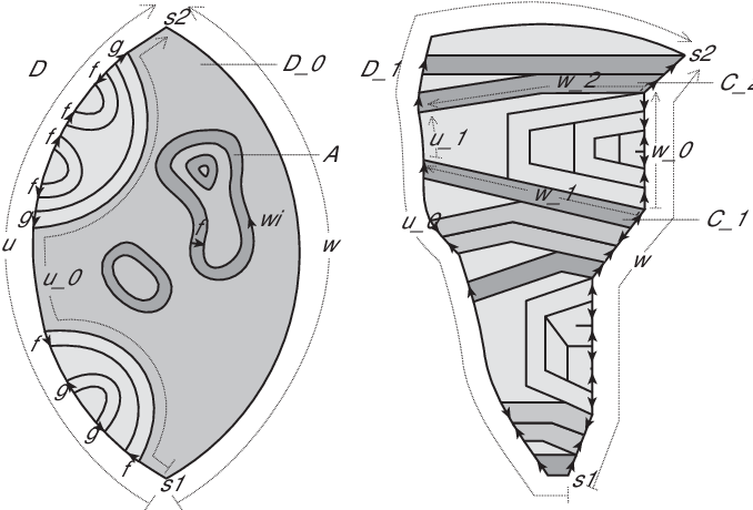
The essential idea in this proof is straightforward: the –corridors (defined in Section 4) emanating from stack up with the length of the corridors growing to roughly at the top of the stack; taking the logarithm of this length gives a lower bound on extrinsic diameter of . However, fleshing this idea out into a rigorous proof requires considerable care.
The first complication we face is that –corridors need not run right across , but can terminate at an edge in the side of an – or – corridor or ring. As every letter in is , the edges of connected in pairs by – and –corridors all lie in . Thus lies in a single connected component of the planar complex obtained by deleting from the interiors and ends of all the – and –corridors. (In the left diagram of Figure 6, is shaded.) Note that . Thus it suffices to prove that . We will do so by considering a further –van Kampen diagram obtained from by removing the interiors of a collection of –disc subdiagrams and gluing in replacement diagrams .
Let be the edge–path in from to such that followed by is the anticlockwise boundary circuit of .
Suppose is an – or –ring in that is not enclosed by another – or –ring. The outer boundary circuit of is labelled by a word in . The retraction of Lemma 3.2 maps to itself and satisfies the hypotheses of Lemma 8.2. So induces a distance decreasing singular combinatorial map from , the diagram enclosed by , onto an –van Kampen diagram. Therefore, without increasing extrinsic diameter, we may assume to be an –diagram. By Lemma 3.3, is null–homotopic in the subpresentation of .
Let be a topological 2–disc van Kampen diagram for in .
We will show that there is an –corridor in with one side labelled by a word such that is large. Recall that each –corridor in a –van Kampen diagram connects two edges that are either in the boundary of the diagram or the boundary of a 2–cell with label . But every such 2–cell is part of an –corridor, and as contains no – or –corridor, each of its –corridors connects two edges in . Each –edge in is part of an –corridor that must either return to or end on . An –corridor of the former type connects two oppositely oriented –edges in . Consider with and running upwards with on the left and on the right (as in Figure 6). So –corridors of the latter type are horizontal, stacked one above another.
Define a horizontal corridor to be an up– or down–corridor according to whether the edge it meets on is oriented upwards or downwards. And call an up–corridor a last–up–corridor when it meets an edge on that is labelled by the final letter of a prefix of with the property that for all prefixes of with . Note that there are exactly last–up–corridors in . In the right diagram of Figure 6 the up– and down–corridors are shaded and the last–up–corridors are darker. That figure also depicts the scenario addressed in the following lemma.
Lemma 5.5
Suppose that and are two horizontal corridors running from to in , that is below , and that there are no horizontal corridors between and . Assume that the subarc of connecting, but not including, the two edges where and meet is labelled by a word . Let and be the words read right to left along the top of and along the bottom of , respectively. Then we have equality of the exponential sums .
Proof of Lemma 5.5. Let be the subarc of connecting, but not including, the two edges where and meet . Let be the subword of that we read along .
Edges labelled by in and by in are the start of –corridors that must return to or , respectively, because there are no horizontal corridors between and . So and freely reduces to the empty word. Moreover in we find that where is obtained from by removing all occurrences . Also, is null–homotopic.
Now as they are the labels of the sides of –corridors and . So by Lemma 3.4, is null–homotopic in
As does not occur in , we deduce that .
Returning to our proof of Proposition 5.4, we note that edges that are part of but not of are labelled by letters in because they are in the sides of – or –corridors. So Lemma 5.5 applies to adjacent horizontal corridors that meet at edges connected by an arc of that does not include edges from . By the pigeonhole principle, there must be a stack of last–up–corridors that all meet a fixed subarc of that includes no edges from . (The stack may also include horizontal corridors that are not last–up–corridors.)
If is a horizontal –corridor and and are the words along the top and bottom sides of , then when is an up–corridor, and when is a down–corridor. Let be the exponent sum of the letters in the word along the bottom edge of the lowest last–up–corridor in . Note that is non–zero because the –corridor’s two ends are labelled differently. The number of up–corridors minus the number of down corridors in is and so by Lemma 5.5, defining to be the word we read along the edge–path along the top of the highest corridor in , we find .
Suppose and are prefixes of . If in then in by Lemma 3.4, and so . So if , then the vertices , of reached after reading and map to different vertices in . So, because and , the number of vertices in the image of in is at least . But we must say more: there are prefixes of that all end and for which are all different. The vertices at the end of the arc labelled by these are not in the interior of any of the diagrams defined prior to Lemma 5.5 (as contain no –edges) — so the number of vertices in the image of in is at least .
The number of vertices in a closed ball of radius in is at most for some constant depending only on the valence of the vertices in , and hence on the number of defining generators in . Thus
5.3 An upper bound for the distortion of in
One conclusion of Proposition 5.1 was that it is possible to express as a word of length . The main result of this section, Proposition 5.7, is that no greater distortion of is possible; this will be crucial in Section 7 when we come to analyse –van Kampen diagrams by breaking them down into – and –subdiagrams meeting along arcs labelled by powers of .
Lemma 5.6
If is a word in the generators of that equals in the group, then
where .
Proof. If we represent elements of as column–vectors, then the actions of and by conjugation are given by left multiplication by the matrices
respectively. Similarly, we can give matrices for the actions of and .
We will inductively obtain words , all of which equal in , as follows. In every van Kampen diagram for , the letters in occur in pairs or connected by –corridors and –corridors. The geometry of these corridors necessitates that have a subword of the form or , where . Obtain from by replacing every letter () in by a word of minimal length in that equals or , as appropriate. Let be the matrix with ones in every entry on and below the diagonal and zeros elsewhere. Comparing with the four matrices discussed above we see that is at most the –th entry in the column vector .
Using the identity
we calculate that
Now and so is at most the –th entry in . The asserted bound follows.
Recall that denotes the exponent sum of letters in .
Proposition 5.7
Suppose is a word equalling in . Let . Then
where is a constant depending only on .
Proof. The retraction of Lemma 3.2 maps , letter–by–letter, to a word equalling in . Each is mapped by to which is central in . So if we define to be the word obtained from by removing all letters and to be the word obtained by applying , letter–by–letter, to then in .
By Lemma 5.6
The asserted bound then follows because, for a suitable constant depending only on , one has for all .
5.4 The intrinsic diameter of diagrams for
The results in this section culminate with an upper bound on the intrinsic diameter functional of . This will be used in Section 7.1, when we establish the upper bound on the extrinsic diameter of .
Lemma 5.8
If is a length word in representing an element of the subgroup or of , then there is a word in or in , respectively, such that in and , where depends only on .
Proof. The retracts of Lemma 3.2 mapping onto and mean that it is enough to prove this lemma for instead of . The result for can be proved in the same manner as Lemma 5.6.
Define
a subpresentation of . Note that the 2–dimensional portions of every –van Kampen are comprised of intersecting –, –, and – rings and corridors (where and ).
Lemma 5.9
If is a minimal area –van Kampen diagram for a word then
- (i)
amongst the corridors and rings in , no two cross twice,
- (ii)
contains no – or –rings (),
- (iii)
contains no –rings,
- (iv)
contains no –rings, and
- (v)
the length of each – and –corridor () in is less than .
Proof. For (i), first suppose that for some with , there is an –corridor or –ring that crosses an –corridor or –ring twice, intersecting at two 2–cells and . Let and be portions of and between (but not including) and , as shown in Figure 7. By an innermost argument we may assume that no –corridor or –ring intersects twice and that no –corridor or –ring intersects twice. Removing and , relabelling all the –edges in by and all the –edges in by , and then gluing up as shown in Figure 7, would produce a van Kampen diagram for of lesser area than . This would contradict the minimality of the area of . (Topologically, the effect of the surgery on is to collapse to points arcs running through and between opposite vertices in and . This does not spoil planarity because no opposite pair of vertices were identified in .)

Next suppose that for some , an –corridor or ring crosses an –corridor or ring twice at 2–cells and . Let and be portions of and between (but not including) and . We may assume that no –corridor or –ring intersects twice and that no –corridor or –ring () intersects twice. Let be the subdiagram between and . For reasons we are about to explain we may assume includes no 2–cells labelled by , (equivalently, contains no –edge). This leads to a contradiction, as above.
No 2–cell of labelled lies in an –corridor, as such a corridor would intersect twice. Also includes no 2–cell that is part of an –ring — such a ring could intersect and so would have to be entirely in ; but then, by another innermost argument, this –ring would only contain 2–cells labelled by as otherwise it would twice intersect an –corridor for some . So includes no 2–cells labelled by , and for similar reasons, no 2–cells labelled by . So all –edges in are identified in pairs and are amongst the 1–dimensional portions of . It follows that there are no –edges in , or there is a –edge in that is connected to the rest of at only one vertex, or there is a 2–disc component of that does not adjoin .
The second case is impossible because it would imply that was not reduced. The third case cannot happen because for some , an –corridor would have to cross , travel through this 2–disc portion and then cross again. Thus has no –edges.
The same arguments tell us that for all , no – and – corridors or rings in can cross twice. No other combination of rings and corridors can cross even once.
Now follows immediately from , as do and in the cases where the rings include 2–cells other than those labelled by or . In the remaining cases the outer boundary of the ring is labelled by a freely reducible word in , which contradicts the minimality of the area of .
For , suppose is an – or –corridor. The boundary circuit of is comprised of the two ends of and two edge–paths, one of which, call it , must have length less than . By (i)–(iv) a different corridor connects each on a side of to . So has length less than .
Lemma 5.10
There exists a constant such that for all .
Proof. Suppose is a minimal area –van Kampen diagram for a word . All –corridors in are embedded: if a portion (of non–zero length) of the path along the side of an –corridor formed an edge–loop then that would have to enclose a zero area subdiagram (by the results of Lemma 5.9) and therefore be labelled by a non–reduced path — but then would not be a minimal area diagram as there would be an inverse pair of 2–cells on the corridor. So from any given vertex in , travelling across –corridors at most times, we meet either an –corridor (), or an –corridor (), or . In the former two cases one can follow a path of length at most along a side of the – or –corridor to . From any point on one can reach the base vertex by following the boundary circuit.
Proposition 5.11
.
Proof. Suppose is a null–homotopic word in and is a van Kampen diagram for . We will construct a new van Kampen diagram for that satisfies the claimed bound on intrinsic diameter. We begin the construction of by taking an edge–circuit of length in the plane to serve as . We direct and label the edges of so that one reads around it.
The occurrences of and in are paired so that the corresponding edges of are joined by corridors in . For each such pair, there must be a subword in some cyclic conjugate of or such that both and represent elements of the subgroup . Join the pairs of – and –edges in by –corridors running through the interior of . It follows from Lemma 5.8 that the lengths of both sides of these –corridors are at most a constant times .
Likewise, insert corridors into the interior of joining pairs of – and –edges, of – and –edges, and of and –edges. There is no obstruction to planarity in the 2–complex because we are mimicking the layout of corridors in .
To complete the construction of , we shall fill the 2–disc holes inside . The boundary circuit of each hole is made up of the sides of corridors and a number of disjoint subarcs of . The length of is at most , up to a multiplicative constant, because these disjoint subarcs contribute at most and the lengths of the sides of each contribute at most a constant times , where . By Lemma 5.10, these circuits can be filled by –van Kampen diagrams with intrinsic diameter at most a constant times . And, as the corridors have length at most a constant times , we deduce that , as required.
Remark 5.12
Let us consider why the Dehn function of is at most for some constant .
Lemma 5.9 implies that the Dehn function of is at most for some : the total contribution of the 2–cells labelled by or for some is at most ; removing all – and –corridors (for all ) leaves components with linear length boundary circuits filled by minimal area van Kampen diagrams over
and a standard corridors argument shows the Dehn function of this subpresentation is bounded above by an exponential function. The construction of diagrams in Proposition 5.11 then establishes that the Dehn function of is at most for some .
6 Diameter in
In this section we establish an upper bound on the intrinsic, and hence extrinsic, diameter of null–homotopic words in the presentation for . Also we show how the shortcuts of Proposition 5.1 lead to an improved bound on extrinsic diameter when we regard as a word in the presentation for .
Proposition 6.1
Fix integers and . Suppose is a null–homotopic word in the presentation for , that , and that . Then there is a –van Kampen diagram for with . Moreover, as an –van Kampen diagram,
To prove this result we will need some purchase on the geometry of – and –corridors. This is provided by the following two lemmas.
Lemma 6.2
Suppose is a minimal area –van Kampen diagram for a null–homotopic word and that is a –corridor in . Let be the word along the sides of . If is a subword of and then cannot represent the same group element as a non–zero power of . In particular, is embedded; that is, the sides of are simple paths in .
Proof. As is of minimal area, is freely reduced as a word in
Killing and retracts onto
in which generate a free subgroup. This retraction sends to a word in that is freely reduced and therefore non–trivial. The result follows.
The analogue of this result for –corridors is more complex.
Lemma 6.3
Suppose is a minimal area –van Kampen diagram for a null–homotopic word and that is a –corridor in . Then is a topological 2–disc subdiagram of with boundary label , where and are freely reduced words in . Moreover, defining and to be the arcs of along which one reads and , there exists , depending only on , such that from any point on () there is a path in of length at most to . Also, no subword of or represents the same group element as a non–zero power of .
Proof. That is reduced, that is a simple path in , and that no subword of or represents the same group element as a non–zero power of , are all proved as in Lemma 6.2. And is a topological 2–disc by a similar argument involving the retraction .
So is obtained from by replacing each by for all , and then freely reducing. The constant exists by the Bounded Cancellation Lemma of [6].
Proof of Proposition 6.1. Let be a –van Kampen diagram for that is of minimal area. Note that contains no –, – or –rings. Removing the – and –corridors from leaves a disjoint union of subdiagrams over
Since there are no –rings in and the words along the sides of the –corridors are reduced, from any vertex in one can reach by following at most –edges across successive –corridors.
We claim that if is a – or –corridor in and is the word along a side of then , where and are the lengths of the two arcs that together comprise and have the same end points as one side of . This is because killing and retracts onto , and the calculation used in the proof of Proposition 5.6 shows that the conjugation action of the stable letter is an automorphism of polynomial growth of degree . And on page 452 of [4] the first author shows that the growth of the inverse automorphism is also polynomial of degree .
It follows that because the boundary of consists of portions of , and the sides of – and –corridors.
We are now ready to estimate . Suppose is a vertex of . In the light of Lemmas 6.2 and 6.3, there is no loss of generality in assuming is not in the interior of a – or –corridor. Move from to by successively crossing – and –corridors as follows. When located on a – or –corridor that has not just been crossed, follow at most (the constant of Lemma 6.3) edges to cross to the other side; otherwise follow a maximal length embedded path of –edges across some . Finally follow to the base vertex . Let denote the resulting edge–path from to .
It must be verified that we can indeed reach by moving in the manner described and that . First note that there are no embedded edge–loops in labelled by words in because the interior of such a loop could be removed and the hole glued up (as retracts onto ), reducing the area of . Next observe that does not cross the same – or –corridor twice, for otherwise there would have to be an innermost – or –corridor that crosses twice, contradicting either Lemma 6.2 or Lemma 6.3.
So crossing the – and –corridors, of which there are at most , contributes at most to the length of . We have already argued that each section of between an adjacent pair of – or –corridors has length . So these sections together contribute at most to the total length. The final section of is part of and so has length at most . The total is as required.
For the bound on , we note that in the word metric (i.e. measured in the Cayley graph) the distance from the initial to the terminal vertex of each arc of whose edges are all labelled by , is by Proposition 5.1. Therefore , as required.
7 Proof of the main theorem
In this section we prove Theorem 7.3 (modulo some technicalities postponed to Section 8). Theorem 1.3 then follows because and can be chosen so that the ratio of the intrinsic and extrinsic diameter filling functionals of grows faster than any prescribed polynomial.
Before stating the theorem we recall the definition of an alternating product expression in an amalgam and a well known lemma — see Lemma 6.4 in Section III. of [5] or Section 5.2 of [9] .
Definition 7.1
Let be an amalgam of groups and along a common subgroup . Suppose and are generating sets for and , respectively. An alternating product expression for is a cyclic conjugate of in which for all we have , , and if then neither nor is the empty word.
Lemma 7.2
In the notation of Definition 7.1, if represents 1 in then in any alternating product expression for , some or represents an element of .
Theorem 7.3
For all integers , the extrinsic and intrinsic diameter filling functions of the group presented by , satisfy
7.1 Proof of the upper bound on
Suppose is a null–homotopic word in . Let be an alternating product decomposition for where each and is a word on the generators of and respectively. Take a planar edge–circuit around which, after directing and labelling the edges, one reads . Decompose into arcs along which we read the and , and call the vertices at which these meet alternation vertices. Say that an edge–path is a –arc when it is made up of –edges orientated the same way.
Repeated appeals to Lemma 7.2, the first of which tells us that some or represents a word in , allow us to deduce that –arcs with the following properties can be inserted into the interior of : each –arc connects two distinct alternation vertices of ; any two –arcs are disjoint; and the –arcs partition the interior of into topological 2–disc regions, whose boundary loops are labelled by words that are null–homotopic either in or in . Call these bounding loops –loops and –loops, respectively.
Lemma 7.4
For each –arc , let be the length of the shorter of the two subarcs of that share their two end vertices with . Then the length of satisfies
where is the constant of Proposition 5.7, which depends only on .

Proof of Lemma 7.4. We induct on . The base case, holds vacuously. For the inductive step, of the two regions adjoining , choose to be that which is in the interior of the disc bounded by and the length subarc of — see Figure 8. The boundary of is comprised of , disjoint subarcs of , and some –arcs that we call . Define to be the total length of these subarcs of . Then
| (2) |
By induction hypothesis, for all . We address two cases.
Case: is a –loop. The exponent sum of the occurrences of in any null–homotopic word in is zero because retracts onto via the map that kills all generators other than . So
with the second inequality following from (2).
This completes the proof of the lemma.
Next we fill the – and –loops inside to produce a van Kampen diagram that satisfies the asserted bound on extrinsic diameter. Let . By Lemma 7.4, the length of each of their boundary circuits is at most , with the contributions from portions not on coming entirely from –arcs. First we fill the –loops as per Proposition 6.1, with diagrams each of which meets and has extrinsic diameter as an –van Kampen diagram.
Next we glue a shortcut diagram along each of the –arcs as per Proposition 5.1. These diagrams have intrinsic diameter , measured from base vertices on . Finally, fill the remaining –loops — all have length and meet , and by Proposition 5.11 they can be filled by van Kampen diagrams of intrinsic, and hence extrinsic, diameter .
The result is an –van Kampen diagram that admits the asserted bound on extrinsic diameter.
7.2 Proof of the lower bound on .
Define
Let be the (positive) word such that in . Define . For some we have . This plays a key role in the construction of the –van Kampen for , an outline for which is shown in Figure 9.

Lemma 7.6
The word has extrinsic diameter at least in , where is a constant depending only on .
Proof of Lemma 7.6. Our approach builds on the proof by the first author of Theorem 3.4 in [2]. Suppose is a –van Kampen diagram for . First we find an edge–path in , along which one reads a word in which the exponent sum of the letters is at least for some constant . A –corridor connects the two letters in , and along each side of this corridor we read a word in that equals in . A –corridor joins the in this latter word to some in . Let be the prefix of such that the letter immediately following is this , and then let be the edge–path along the side of the –corridor running from the vertex at the end of to the vertex at the end of . Let be the word one reads along . Then in . Killing , and , retracts onto
in which , where . By Lemma 3.5, the exponent sum of in , and hence of in , is , which is at least for some constant depending only on .
Killing all generators other than defines a retraction of onto . The 0–skeleton of is and the existence of shows that image of has diameter at least , since the retraction from the 0–skeleton of to decreases distance. This completes the proof of the lemma.
Let be a minimal intrinsic diameter –van Kampen diagram for . On account of the retraction , we may assume to have the properties described in Proposition 8.4 (2). That is, the –cells within comprise a subcomplex whose connected components are all simply connected unions of topological disc subcomplexes any two of which meet at no more than one vertex. Refer to these topological disc subcomplexes as –islands. Around the boundary of each –island we read a word in that freely reduces to the empty word because has infinite order in .
We obtain a –van Kampen diagram for from by cutting out the –islands and then gluing up the attaching cycles by identifying adjacent, oppositely–oriented edges (i.e. successively cancelling pairs or in the attaching words). The removal of the –islands and subsequent gluing is described by a collapsing map that is injective and combinatorial except on the –islands. This is depicted in Figure 10. Note that, no matter what choice of we make, will be planar by Lemma 8.1, since after cutting out and gluing up a number of the –islands, the boundary circuit of every remaining –island is a simple loop.
Let be a maximal geodesic tree in the 1–skeleton of , based at . Suppose is a geodesic in from a vertex not in the interior of a –island to . Define an edge–path in the 1–skeleton of from to to follow the arcs of outside the interior of –islands, and to follow the geodesic path in the tree whenever enters a –island .
It will be important (in Case 2 below) that the arcs of defined as geodesics in the images of the boundaries of –islands follow edge–paths labelled by reduced words in . That is, they must not traverse a pair of edges labelled by or . The gluing involved choices that, according to the following lemma (illustrated in Figure 10), we can exploit to ensure that the paths satisfy the conditions we require.

Lemma 7.7
The gluing map can be chosen so as to satisfy the following. Suppose is an edge–path in from a vertex to a vertex and is an initial segment of some geodesic in from to . Assume, further, that lies in some –island and meets at and and nowhere else. Define to be the geodesic in the tree from to . Then along we read a reduced word in .
Proof. Start with any choice of gluing map . Suppose that is a –island in and that are as per the lemma, but that follows a word in that incudes an inverse pair, or . Then perform a diamond move as illustrated in Figure 11 to remove the inverse pair. This, in effect, amounts to changing the choice of .

Suppose that are another pair as per the lemma. We claim that when we do the diamond move to remove a pair of edges from the effect, if any, on the word one reads along is also the removal of an inverse pair. Consider the ways in which could meet the pair of edges on which the diamond move is to be performed. The danger is that an inverse pair might be inserted into the word along . But this could only happen when crosses at the vertex between the two edges, and such crossing is impossible because and are both part of geodesic arcs based at in the tree .
There are only finitely many pairs on . So after a finite number of diamond moves, is transformed to a map that satisfies the requirements of the lemma.
Returning once more to the proof of the theorem, let be a vertex in for which and let be a vertex of such that . Let be the geodesic in from to . And let be the edge–path from to , obtained by connecting up the images under of the portions of not in the interior of –islands with geodesic edge–paths in the trees . So is a concatenation of two types of geodesic arcs: those that run through the image under of the boundary of some –island (call these island arcs), and those arcs from .
We fix and examine the following two cases.
- Case 1)
The island–arcs all have length at most .
In place of each island–arc in , we find an arc in of length at least one (in fact, this is a crude lower bound) because the word along each such arc in equals some non–zero power of in . So and therefore , because is a geodesic in , based at .
- Case 2)
Some island–arc through , where is some –island in , has length more than .
Let be the corresponding subarc of through . If then it follows immediately that .
Assume that . Then divides into two subdiagrams each of which has boundary circuit made up of together with a portion of around which we read a word in with exponent sum more than . Applying Proposition 5.4 to either of these two subdiagrams we learn that the intrinsic diameter of is at least a constant times .
So
and taking and we finally have our result.
8 Amalgams and retractions
The main results in this section concern amalgams (that is, free products with amalgamation). But first we give some technical results on cutting, gluing and collapsing operations on 2–complexes. We perform such operations on van Kampen diagrams and our concern is that planarity should not be lost.
The proof of the following lemma is straight–forward and we omit it.
Lemma 8.1
Suppose that is a finite, combinatorial complex embedded in the plane and that is the (not necessarily embedded) edge–circuit in around the boundary of the closure of a component of for which is compact.
- 1.
If is a topological 2–disc combinatorial complex with , then gluing to by identifying the boundary circuit of with produces a planar 2–complex.
- 2.
If is simple and is a planar contractible combinatorial 2–complex with , then gluing to by identifying the boundary circuit of with gives a planar 2–complex.
- 3.
Identifying two adjacent edges and in , as illustrated in Figure 12, produces a planar 2–complex unless and together comprise the boundary of a subdiagram of (as in the rightmost diagram of the figure).

A singular combinatorial map from one complex to another is a continuous map in which every closed –cell is either mapped homeomorphically onto an –cell or is mapped onto .
We leave the proof of the following technical lemma to the reader.
Lemma 8.2
Let and be finite presentations. Suppose is a map and let be the extension of defined by
Suppose that for all , the word is either freely reducible or has a cyclic conjugate in .
If is a –van Kampen diagram for a word , then there is a singular combinatorial map to a –van Kampen diagram for that is distance decreasing with respect to the path metrics on and . Moreover, suppose is an edge of labelled by and is not a single vertex; if then preserves the orientation of and is labelled by , and if then reverses the orientation of and is labelled by .
Corollary 8.3
In addition to the hypotheses of Lemma 8.2 assume that is a subpresentation of . If is a null–homotopic word in , and if , then there is a –van Kampen diagram for that is of minimal intrinsic diameter (or radius) amongst all –van Kampen diagrams for .
In the following proposition, the hypothesis that no cyclic conjugate of a word in is in is mild. It could only fail for freely reducible words in . It allows the 2–cells of a –van Kampen to be partitioned into –cells and –cells; that is, 2–cells that have boundary words in or in , respectively. Note that whenever an –cell shares an edge with an –cell, that edge is labelled by .
Proposition 8.4
Let and be presentations of groups and , such that , where has infinite order in both and . The amalgam has presentation . Assume that no cyclic conjugate of a word in is in .
Suppose that retracts to via a homomorphism that maps to and maps all other to or .
- 1.
Suppose is a null–homotopic word in . Then has an –van Kampen diagram that is of minimal intrinsic diameter (or radius) amongst all –van Kampen diagrams for .
- 2.
Suppose is a null–homotopic word in . Then has a minimal intrinsic diameter –van Kampen diagram such that whenever is a simple edge–circuit in around which we read a word in , the subdiagram it bounds is an –van Kampen diagram.
Proof. The first part is a consequence of Corollary 8.3. For the second part we take a –van Kampen diagram for of minimal intrinsic diameter and obtain a –van Kampen diagram for with the required properties by repeating the following procedure.
Suppose is a simple edge–circuit in around which we read a word in . Let be the word we read around , and let be the –van Kampen subdiagram bounded by . Glue the –van Kampen diagram for supplied by Lemma 8.2, in place of . This does not increase intrinsic diameter because the map of Lemma 8.2 is distance decreasing. Also the gluing cannot destroy planarity because is simple — see Lemma 8.1 (2).
9 Quasi–isometry invariance
A special case of the following theorem is that for any two finite presentations of the same group, and .
Theorem 9.1
If and be finite presentations for quasi–isometric groups and , respectively, then and .
Proof. The theorem is proved by keeping track of diameters as one follows the standard proof that finite presentability is a quasi–isometry invariant [5, page 143]. The first quantified version of this proof (in the context of Dehn functions) appeared in [1].
Fix word metrics and for and , respectively, and quasi–isometries and with constants and , such that for all and all ,
| (3) | |||||
| (4) | |||||
| (5) |
Suppose is an edge–circuit in the Cayley graph , visiting vertices in order. Consider the circuit in obtained by joining by geodesics of length at most , using (4). Fill with a minimal–intrinsic–diameter van Kampen diagram . Extend by joining the images of adjacent vertices by geodesics in , each of length at most by (3), to give a combinatorial map from the 1–skeleton of a diagram obtained by subdividing each of the edges of . Each 2–cell in has boundary length at most . Extend to a map filling by joining each vertex on to on by a geodesic, which has length at most by (5). So is obtained from by attaching a collar of 2–cells around its boundary. Adjacent vertices in are mapped by to vertices at most apart by (4) and then by to vertices at most by (3). So the lengths of the boundaries of the 2–cells in the collar are each at most .
It follows that if we define to be the set of all null–homotopic words in of length at most then extends to a van Kampen diagram filling , where . So is a finite presentation for . Now, and so is at most . By (3) we can multiply this by to get an upper bound on the intrinsic diameter of . Adding a further for the collar, we get
| (6) |
which establishes for this particular .
However, the theorem concerns arbitrary for which is a finite presentation for . The boundary of each 2–cell of is mapped by to an edge–circuit in of length at most . So, to make into a van Kampen diagram over , we fill each of its 2–cells with a (possibly singular) van Kampen diagram over . But, a technical concern here is that gluing a singular 2–disc diagram along a non–embedded edge–circuit of could destroy planarity. The way we deal with this is to fill the 2–cells of one at a time. And, on each occasion, if the 2–cell to be filled has non–embedded boundary circuit then we discard all the edges inside the simple edge–circuit in such that no edge of is outside , and then we fill .
Discarding the edges inside all such does not stop the estimate (6) holding. Adding to account for each of the fillings gives an upper bound on and so . Interchanging the roles of and , we immediately deduce that and so we have , as required.
That can be proved the same way, except we take to be a minimal–extrinsic–diameter filling of , and then by (3)
and adding a further constant gives an upper bound on .
References
- [1] J. M. Alonso. Inégalitiés isopérimétriques et quasi-isométries. C.R. Acad. Sci. Paris Ser. 1 Math., 311:761–764, 1990, MR1082628, Zbl 0726.57002
- [2] M. R. Bridson. Asymptotic cones and polynomial isoperimetric inequalities. Topology, 38(3):543–554, 1999, MR1670404, Zbl 0929.20032
- [3] M. R. Bridson. The geometry of the word problem. In M. R. Bridson and S. M. Salamon, editors, Invitations to Geometry and Topology, pages 33–94. O.U.P., 2002, MR1967746, Zbl 0996.54507
- [4] M. R. Bridson. Polynomial Dehn functions and the length of asynchronously automatic structures. Proc. London Math. Soc., 85(2):441–465, 2002, MR1912057, Zbl 1046.20027
- [5] M. R. Bridson and A. Haefliger. Metric Spaces of Non-positive Curvature. Number 319 in Grundlehren der mathematischen Wissenschaften. Springer Verlag, 1999, MR1744486, Zbl 0988.53001
- [6] D. Cooper. Automorphisms of free groups have finitely generated fixed point sets. J. Algebra, 111:453–456, 1987, MR0916179, Zbl 0628.20029
- [7] M. Gromov. Asymptotic invariants of infinite groups. In G. Niblo and M. Roller, editors, Geometric group theory II, number 182 in LMS lecture notes. Camb. Univ. Press, 1993, MR1253544, Zbl 0841.20039
- [8] M. Gromov. Metric structures for Riemannian and non-Riemannian spaces, volume 152 of Progress in Mathematics. Birkhäuser Boston Inc., Boston, MA, 1999. Based on the 1981 French original, With appendices by M. Katz, P. Pansu and S. Semmes, Translated from the French by S. M. Bates, MR1699320, Zbl 1113.53001
- [9] J.-P. Serre. Trees. Springer Monographs in Mathematics. Springer-Verlag, 2003. Translated from the French original by J. Stillwell, Corrected 2nd printing of the 1980 English translation, MR1954121, Zbl 1013.20001
Martin R. Bridson
Mathematical Institute, 24–29 St Giles’, Oxford, OX1 3LB,
UK
bridson@maths.ac.uk, http://people.maths.ox.ac.uk/bridson/
Timothy R. Riley
Department of Mathematics, University Walk, Bristol, BS8 1TW, UK
tim.riley@bristol.ac.uk, http://www.maths.bris.ac.uk/matrr/