Realizations of the associahedron and cyclohedronThanks: Hohlweg is partially supported by CRC. This work was done during the time both authors were at the Institut Mittag-Leffler, Djursholm, Sweden.

Christophe Hohlweg Christophe HohlwegThe Fields Institute
222 College Street
Toronto, Ontario, M5T 3J1
CANADA Email address: chohlweg@fields.utoronto.ca URL: http://www.fields.utoronto.ca/˜chohlweg and Carsten Lange Carsten LangeFreie Universität Berlin
FB Mathematik und Informatik
Arnimallee 3
14195 Berlin,
GERMANY Email address: lange@math.tu-berlin.de

Date: September 14, 2006

Abstract.

We describe many different realizations with integer coordinates for the associahedron (i.e. the Stasheff polytope) and for the cyclohedron (i.e. the Bott-Taubes polytope) and compare them to the permutahedron of type A and B respectively.

The coordinates are obtained by an algorithm which uses an oriented Coxeter graph of type ${\textnormal{A}}_{n}$ or ${\textnormal{B}}_{n}$ as only input data and which specializes to a procedure presented by J.-L. Loday for a certain orientation of ${\textnormal{A}}_{n}$ . The described realizations have cambrian fans of type A and B as normal fan. This settles a conjecture of N. Reading for cambrian lattices of these types.

1. Introduction

The associahedron ${\mathsf{Asso}}({\textnormal{A}}_{n-1})$ was discovered by J. Stasheff in 1963 [27] and is of great importance in the theory of operads. It is a simple $(n-1)$ -dimensional convex polytope whose $1$ -skeleton is isomorphic to the undirected Hasse diagram of the Tamari lattice on the set ${\mathcal{T}}_{n+2}$ of triangulations of an $(n+2)$ -gon (see for instance [16]) and therefore a fundamental example of a secondary polytope as described in [13]. Numerous realizations of the associahedron have been given, see [6, 17] and the references therein.

An elegant and simple realization of the associahedron by picking some of the inequalities for the permutahedron is due to S. Shnider & S. Sternberg [25] (for a corrected version consider J. Stasheff & S. Shnider [28, Appendix B]). The removed inequalities are related to the vertices by a well-known surjection from $S_{n}$ to the set $Y_{n}$ of planar binary trees that relates the weak order of ${\textnormal{A}}_{n-1}$ with the Tamari lattice as described in [2, Sec. 9]. J.-L. Loday presented recently an algorithm to compute the coordinates of this realization, [17]: label the vertices of the associahedron by planar binary trees with $n+2$ leaves and apply a simple algorithm on trees to obtain integer coordinates in $\mathbbm{R}^{n}$ .

The associahedron fits, up to combinatorial equivalence, in a larger family of polytopes discovered by S. Fomin and A. Zelevinsky [11] (and realized as convex polytopes by F. Chapoton, S. Fomin, and A. Zelevinsky [6]) that is indexed by the elements in the Cartan-Killing classification. Among these generalized associahedra, the cyclohedron ${\mathsf{Asso}}({\textnormal{B}}_{n})$ was first described by R. Bott and C. Taubes in 1994 [4] in connection with knot theory and rediscovered independently by R. Simion [26]. It is a simple $n$ -dimensional convex polytope whose vertices are given by the set ${\mathcal{T}}_{n+2}^{B}$ of centrally symmetric triangulations of a $(2n+2)$ -gon. Various realizations have also been given in [6, 9, 19, 23, 26], but none of them is similar to Loday’s realization.

It is a natural question to ask for a construction similar to Loday’s for the cyclohedron and we present such a construction in this article: Starting with a realization of the permutahedron ${\mathsf{Perm}}({\textnormal{B}}_{n})$ , i.e. the convex hull of the orbit of the point $(1,2,\ldots,2n)$ with respect to the action of the hyperoctahedral group, we give an explicit description of realizations of the cyclohedron by removing facets of ${\mathsf{Perm}}({\textnormal{B}}_{n})$ . Moreover we introduce an algorithm to obtain (integer) coordinates for the vertices of these realizations.

It should also be mentioned that the associahedron and cyclohedron fit into another large family of polytopes, the graph associahedra introduced by M. Carr and S. Devadoss [5] and by M. Davis, T. Januszkiewicz, and R. Scott [8] in the study of real blow-ups of projective hyperplane arrangements. Generalized associahedra and graph associahedra fit into the class of generalized permutahedra of A. Postnikov [21] where the right-hand sides for the facet inequalities of the permutahedron ${\mathsf{Perm}}({\textnormal{A}}_{n-1})$ are altered. In fact, the associahedron and cyclohedron can be obtained from this permutahedron by changing the right-hand side of some facet inequalities as described for example by Postnikov [21]. This description of the cyclohedron is obtained from “cyclic intervals of $[n]$ ”, that is, the cyclohedron is seen as “graph associahedron of a cycle”. On the contrary, the realizations given in this article see the associahedron and cyclohedron related to the Coxeter graph of type $A$ and $B$ . The associahedron and cyclohedron may be obtained in many ways by omission of some inequalities. We explicitly describe possible choices for these facet inequalities related oriented Coxeter graphs of type $A$ and $B$ and the resulting coordinates. Moreover, the presented realizations of the cyclohedron are the first explicit realizations as a “generalized type $B$ permutahedron”, i.e. the cyclohedron is obtained from the permutahedron of type $B$ by changing the right hand side of some inequalities.

It turns out that Loday’s construction is generalized in two ways by our algorithm: Firstly, for a certain orientation of the Coxeter graph of type $A$ our algorithm coincides with his construction and secondly, our algorithm also works for the type B associahedron, it yields coordinates for the cyclohedron for any oriented Coxeter graph of type $B$ .

In §1.1 and §1.2 we explain our algorithm and realizations of the associahedron and of the cyclohedron and state the main results. These results are proved in §2 and §3 by explicitly stating a H-representation¹¹ 1 There are two ways to realize a polytope: The H-representation is the intersection of a finite number of closed half spaces and the V-description is the convex hull of a finite number of points, see Ziegler [30] for further deatils. for each realization. Finally in §4 we comment some observations concerning isometry classes and barycenters of these realizations. Moreover, in this section we show that the normal fans of the realizations we provide coincide with the cambrian fans of type $A$ and $B$ . We settle therefore Conjecture 1.1 of N. Reading [22] in type $A$ and $B$ .

N.B. We remark that our construction yields polytopes with the combinatorial type of the generalized associahedra of type $A_{n}$ and $B_{n}$ . It might be worth to mention that the combinatorics of all the polytopes involved is determined by their $1$ -skeleton or graph, since these polytopes are simple. This was shown by R. Blind and P. Mani-Levitska, [3], as well as by G. Kalai, [14].

1.1. Realizations of the associahedron

Let $S_{n}$ be the symmetric group acting on the set $[n]=\{1,\dots,n\}$ . As a Coxeter group of type $A_{n-1}$ , $S_{n}$ is generated by the simple transpositions $\tau_{i}=(i,i+1)$ , $i\in[n-1]$ . The Coxeter graph ${\textnormal{A}}_{n-1}$ is then

Let ${\mathscr{A}}$ be an orientation of ${\textnormal{A}}_{n-1}$ . Following N. Reading, we distinguish between up and down elements of $\{2,\ldots,n-1\}$ : An element $i\in\{2,\ldots n-1\}$ is up if the edge $\{\tau_{i-1},\tau_{i}\}$ is directed from $\tau_{i}$ to $\tau_{i-1}$ and down otherwise. We extend this definition to $[n]$ by the convention that $1$ and $n$ are always down. We remark that in Reading’s work $1$ and $n$ can be chosen to be up or down. Let ${\mathsf{D}}_{\mathscr{A}}$ be the set of down elements and ${\mathsf{U}}_{\mathscr{A}}$ be the set of up elements (possibly empty).

The notion of up and down induces a labelling of a fixed convex $(n+2)$ -gon $P$ as follows: label one vertex of the $(n+2)$ -gon by $0$ . The adjacent vertex in counterclockwise direction is labelled by the smallest down element of $[n]$ not already used. Repeat this procedure as long as there is a down element that has not been used. If there is no such element use label $n+1$ and continue to label the next counterclockwise element by the largest up element of $[n]$ that has not been used so far and iterate. An example is given in Figure 1.

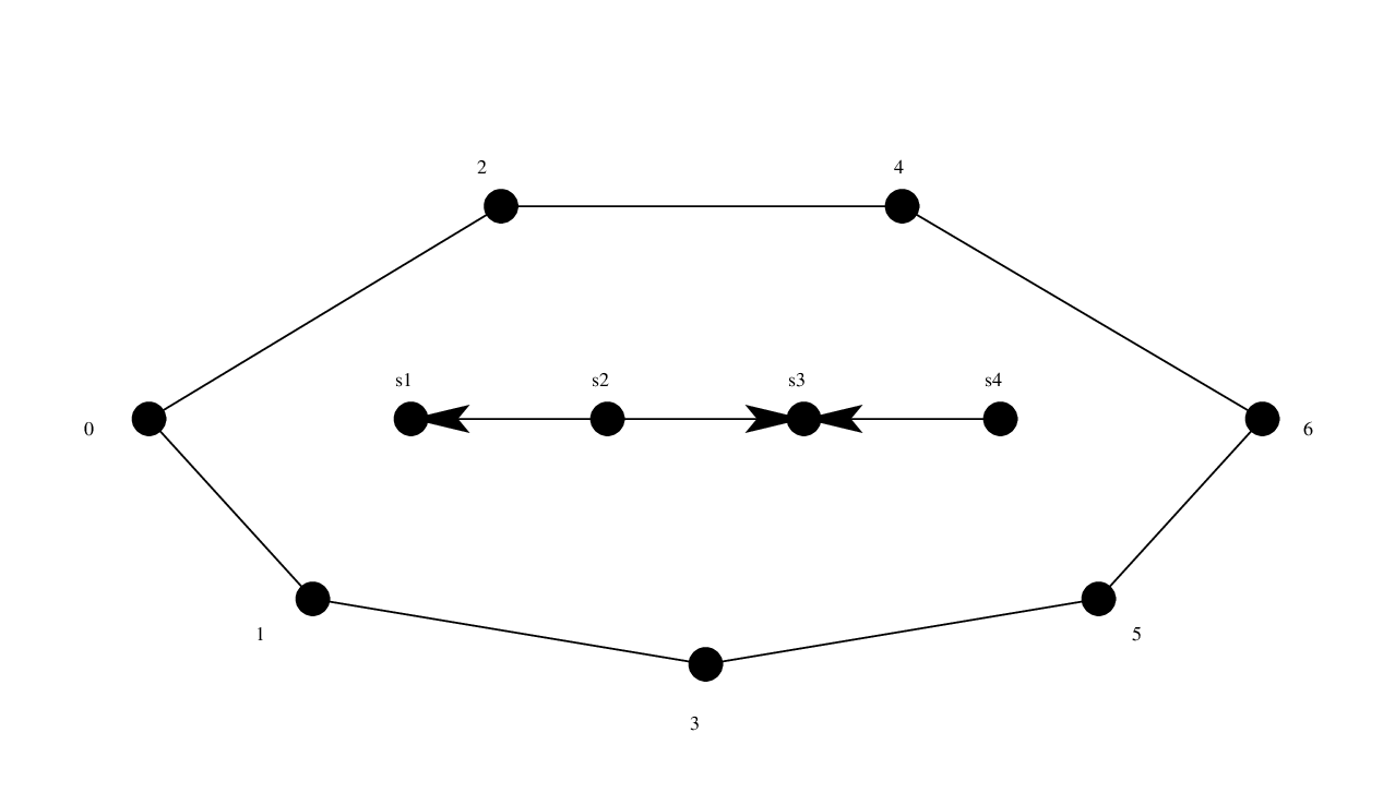
Refer to caption — Figure 1. A labelling of a heptagon that corresponds to the orientation ${\mathscr{A}}$ on ${\textnormal{A}}_{4}$ shown inside the heptagon. We have ${\mathsf{D}}_{{\mathscr{A}}}=\{1,3,5\}$ and ${\mathsf{U}}_{{\mathscr{A}}}=\{2,4\}$ .

Now we consider $P$ labelled according to a fixed orientation ${\mathscr{A}}$ . A triangulation $T$ of $P$ is a planar graph with vertex set the vertices of $P$ and edge set the edges of $P$ and $n-1$ non-crossing diagonals different from the boundary edges. We denote by ${\mathcal{T}}_{n+2}$ the set of all triangulations of $P$ and describe a triangulation by its non-crossing diagonals. Our goal is now to define an injective map

	$\displaystyle M_{{\mathscr{A}}}:{\mathcal{T}}_{n+2}$	$\displaystyle\longrightarrow\mathbbm{R}^{n}$
	$\displaystyle T$	$\displaystyle\longmapsto(x_{1},x_{2},\dots,x_{n})$

that assigns explicit coordinates to a triangulation.

Before we define $M_{{\mathscr{A}}}$ , we introduce a family of functions $\mu_{i}:\{0,1,\dots,n+1\}\to[n+2]$ that measure distances between labels of $P$ and that is parameterized by $i\in[n]$ . For $j<i$ , $\mu_{i}(j)$ counts the number of edges $\{a,b\}$ of the path (on the boundary of $P$ ) connecting $i$ and $j$ that uses only labels $\leq i$ . For $j\geq i$ , $\mu_{i}(j)$ counts the number of edges $\{a,b\}$ of the path (on the boundary of $P$ ) connecting $i$ and $j$ that uses only labels $\geq i$ . For instance, we have $\mu_{4}(5)=2$ and $\mu_{5}(4)=5$ in Figure 1.

\begin{overpic}[pics/a3_associahedra_new.eps] \put(15.0,1.3){$T_{1}=\ $\tiny$0$} \put(25.0,-1.3){\tiny$1$} \put(25.0,3.7){\tiny$2$} \put(28.5,-1.3){\tiny$3$} \put(30.0,1.3){\tiny$4$} \put(28.5,3.7){\tiny$5$} \put(14.0,38.4){$T_{3}=\ $\tiny$0$} \put(24.0,36.0){\tiny$1$} \put(24.0,41.1){\tiny$2$} \put(27.5,36.0){\tiny$3$} \put(29.0,38.4){\tiny$4$} \put(27.5,41.1){\tiny$5$} \put(69.0,1.3){$T_{2}=\ $\tiny$0$} \put(79.0,-1.3){\tiny$1$} \put(79.0,3.7){\tiny$2$} \put(82.5,3.7){\tiny$3$} \put(82.5,-1.3){\tiny$4$} \put(84.0,1.3){\tiny$5$} \put(69.0,38.4){$T_{4}=\ $\tiny$0$} \put(79.0,36.0){\tiny$1$} \put(79.0,41.1){\tiny$2$} \put(82.5,41.1){\tiny$3$} \put(82.5,36.0){\tiny$4$} \put(84.0,38.41){\tiny$5$} \end{overpic}

Figure 2. The vertices of the two associahedra shown have coordinates that are computed from triangulations of labelled hexagons.

For a triangulation $T\in{\mathcal{T}}_{n+2}$ of $P$ and $i\in[n]$ , we denote by ${\mathsf{L}}^{T}_{i}$ the set $\left\{a\vphantom{0\leq a<i\text{ and }\{a,i\}\in T}\right.\;\left|\;\vphantom{a}0\leq a<i\text{ and }\{a,i\}\in T\right\}$ and by ${\mathsf{R}}^{T}_{i}$ the set $\left\{b\vphantom{i<b\leq n+1\text{ and }\{b,i\}\in T}\right.\;\left|\;\vphantom{b}i<b\leq n+1\text{ and }\{b,i\}\in T\right\}$ . Set

p_{\ell}^{T}(i):=\max_{a\in{\mathsf{L}}_{i}^{T}}\ \{\mu_{i}(a)\}\qquad\textrm{and}\qquad p_{r}^{T}(i):=\max_{b\in{\mathsf{R}}_{i}^{T}}\ \{\mu_{i}(b)\}.

The weight $\omega_{i}$ of $i$ in $T$ is the integer $p_{\ell}^{T}(i)p_{r}^{T}(i)$ . We now define the coordinates $x_{i}$ of $M_{{\mathscr{A}}}(T)$ :

x_{i}:=\begin{cases}\omega_{i}&\textrm{if }i\in{\mathsf{D}}_{\mathscr{A}}\\ n+1-\omega_{i}&\textrm{if }i\in{\mathsf{U}}_{\mathscr{A}}.\end{cases}

In the setting of Figure 2, let ${\mathscr{A}}_{1}$ denote the orientation that yields the realization on the left and ${\mathscr{A}}_{2}$ denote the orientation that yields the realization on the right. Consider the triangulations $T_{1}=\{\{0,3\},\{2,3\},\{2,4\}\}$ , $T_{2}=\{\{0,4\},\{2,4\},\{3,4\}\}$ , $T_{3}=\{\{1,2\},\{1,5\},\{3,5\}\}$ , and $T_{4}=\{\{1,2\},\{1,3\},\{1,5\}\}$ that are given by their set of diagonals ( $T_{1},T_{3}$ are triangulations of the left hexagon while $T_{2},T_{4}$ are triangulations of the right hexagon). Then

M_{{\mathscr{A}}_{1}}(T_{1})=M_{{\mathscr{A}}_{2}}(T_{2})=(1,2,3,4)\qquad\text{and}\qquad M_{{\mathscr{A}}_{1}}(T_{3})=M_{{\mathscr{A}}_{2}}(T_{4})=(4,3,2,1).

Theorem 1.1.

Fix an orientation ${\mathscr{A}}$ on ${\textnormal{A}}_{n-1}$ . The convex hull of $\left\{M_{{\mathscr{A}}}(T)\vphantom{T\in{\mathcal{T}}_{n+2}}\right.\;\left|\;\vphantom{M_{{\mathscr{A}}}(T)}T\in{\mathcal{T}}_{n+2}\right\}$ is a realization of the associahedron ${\mathsf{Asso}}({\textnormal{A}}_{n-1})$ with integer coordinates.

This V-representation of ${\mathsf{Asso}}({\textnormal{A}}_{n-1})$ as convex hull of vertices is proved in Section 2.

Remark 1.2.

If all edges of ${\textnormal{A}}_{n-1}$ are directed from left to right, then the realization just described coincides with the one given by Loday. In this situation, ${\mathsf{U}}_{{\mathscr{A}}}=\varnothing$ . Let $T\in{\mathcal{T}}_{n+2}$ and for each $i\in[n]$ , let $a$ and $b$ be such that $p_{\ell}^{T}(i)=\mu_{i}(a)$ and $p_{r}^{T}(i)=\mu_{i}(b)$ . Consider the triangle $\{a,i,b\}$ . Label this triangle by $i$ . Now, take the dual graph of $T$ : it is a planar binary tree with $n+1$ leaves whose root is determined by the edge $\{0,n+1\}$ of $T$ and whose internal nodes are labelled by the label of the corresponding triangle. Then for each $i\in[n]$ the weight $\omega_{i}$ of $i$ is the product of the leaves of the left side of $i$ and of the leaves of the right side. That is precisely how J.-L. Loday computes the coordinates of the vertices in his realization, starting from planar binary trees.

We are now interested in a surjective map

\Phi_{\mathscr{A}}:S_{n}\to{\mathcal{T}}_{n+2}

for any given orientation ${\mathscr{A}}$ of ${\textnormal{A}}_{n-1}$ . These maps have been used earlier. L. Billera & B. Sturmfels used them in [1] where associahedra are described as iterated fibre polytopes. Other references are V. Reiner [23], A. Björner & M. Wachs [2, Remark 9.14], J.-L. Loday & M. Ronco, [18], A. Tonk, [29], and N. Reading [22], who used this family of maps in his study of cambrian lattices of type $A$ . The orientation ${\mathscr{A}}$ where each edge of $A_{n-1}$ is oriented from left to right yields a well-studied map that turns out to be a lattice epimorphism from the (right) weak order lattice to the Tamari lattice. In fact, the undirected Hasse diagram of a cambrian lattice of type $A$ is combinatorially equivalent to the $1$ -skeleton of ${\mathsf{Asso}}({\textnormal{A}}_{n-1})$ [22, Theorem 1.3]. In other words, these maps can be viewed as ‘ $1$ -skeleton’ maps from ${\mathsf{Perm}}({\textnormal{A}}_{n-1})$ to ${\mathsf{Asso}}({\textnormal{A}}_{n-1})$ .

We follow the procedure given in [22] by N. Reading to describe these maps $\Phi_{{\mathscr{A}}}$ . We remark that N. Reading uses the left weak order while we prefer the right weak order. So we invert $\sigma\in S_{n}$ to translate between left and right weak order. Let $\sigma\in S_{n}$ and start with the path of the labelled $(n+2)$ -gon that connects $0$ with $n+1$ and passes through all down elements. Now read the permutation $\sigma^{-1}$ (represented as a word in $[n]$ ) from left to right and construct inductively a new path from $0$ to $n+1$ : If the next letter of $\sigma^{-1}$ is a down element then delete this element in the path; if the next letter is an up element then insert this element between its largest predecessor and its smallest successor in the path. The edges used during this process define a triangulation $\Phi_{\mathscr{A}}(\sigma)$ of the labelled $(n+2)$ -gon, see Figure 3 for an example.

The permutahedron ${\mathsf{Perm}}({\textnormal{A}}_{n-1})$ is the classical permutahedron $\Pi_{n-1}$ which is defined as the convex hull of the points

M(\sigma):=(\sigma(1),\sigma(2),\dots,\sigma(n))\in\mathbbm{R}^{n},\qquad\forall\sigma\in S_{n}.

The idea of S. Shnider & S. Sternberg to obtain the associahedron from the permutahedron by discarding inequalities extends to all realizations of the associahedron of Theorem 1.1. The map $K_{{\mathscr{A}}}$ assigns subsets of $[n-1]$ to a diagonal and is defined in Section 2.

Proposition 1.3.

Fix an orientation ${\mathscr{A}}$ . The associahedron of Theorem 1.1 is given by a subset of the inequalities for the permutahedron ${\mathsf{Perm}}({\textnormal{A}}_{n-1})$ . These inequalities are determined by the image under $K_{{\mathscr{A}}}$ of the diagonals of the $(n+2)$ -gon labelled according to ${\mathscr{A}}$ .

Moreover, the following analog to [17, Proposition 2] shows that our realizations are closely related to the maps $\Phi_{{\mathscr{A}}}$ : A triangulation $T$ has a singleton $\{\sigma\}=(\Phi_{{\mathscr{A}}})^{-1}(T)$ as preimage if and only if $M_{{\mathscr{A}}}(T)$ is a vertex of the permutahedron ${\mathsf{Perm}}({\textnormal{A}}_{n-1})$ . But there are more ways to characterize the common vertices of the associahedron and permutahedron which depend on a chosen orientation ${\mathscr{A}}$ .

Proposition 1.4.

Fix an orientation ${\mathscr{A}}$ on ${\textnormal{A}}_{n-1}$ and let $T\in{\mathcal{T}}_{n+2}$ and $\sigma\in S_{n}$ . The following statements are equivalent:

(a)

$M_{{\mathscr{A}}}(T)=M(\sigma)$ ,
(b)

$\Phi_{{\mathscr{A}}}(\sigma)=T$ and the diagonals of $T$ can be labelled such that

$\varnothing\subset K_{{\mathscr{A}}}(D_{1})\subset\ldots\subset K_{{\mathscr{A}}}(D_{n-1})\subset[n]$

is a sequence of strictly increasing nested sets.
(c)

$(\Phi_{{\mathscr{A}}})^{-1}(T)=\{\sigma\}$ ,
(d)

$\Phi_{{\mathscr{A}}}(\sigma)=T$ and for each $i\in[n]$ we have $p_{\ell}^{T}(i)=1$ or $p_{r}^{T}(i)=1$ .

The proof of both propositions is postponed to Section 2.

1.2. Realizations of the cyclohedron

An orientation ${\mathscr{A}}$ of ${\textnormal{A}}_{2n-1}$ is symmetric if the edges $\{\tau_{i},\tau_{i+1}\}$ and $\{\tau_{2n-i-1},\tau_{2n-i}\}$ are oriented in opposite directions for all $i\in[2n-2]$ . There is a bijection between the symmetric orientations of ${\textnormal{A}}_{2n-1}$ and the orientations ${\mathscr{B}}$ of the Coxeter graph ${\textnormal{B}}_{n}$ that we describe below. A triangulation $T\in{\mathcal{T}}_{2n+2}$ is centrally symmetric if $T$ , viewed as a triangulation of a regular $(2n+2)$ -gon, is centrally symmetric. Let ${\mathcal{T}}_{2n+2}^{B}$ be the set of the centrally symmetric triangulations of the labelled $(2n+2)$ -gon.

Theorem 1.5.

Let ${\mathscr{A}}$ be a symmetric orientation of ${\textnormal{A}}_{2n-1}$ . The convex hull of $\left\{M_{{\mathscr{A}}}(T)\vphantom{T\in{\mathcal{T}}^{B}_{2n+2}}\right.\;\left|\;\vphantom{M_{{\mathscr{A}}}(T)}T\in{\mathcal{T}}^{B}_{2n+2}\right\}$ is a realization of the cyclohedron ${\mathsf{Asso}}({\textnormal{B}}_{n})$ with integer coordinates.

A proof of Theorem 1.5 is be given in Section 3, examples are shown in Figures 4 and 5. The latter shows a realization of ${\mathsf{Asso}}({\textnormal{B}}_{3})$ together with a table of the coordinates of its vertices and the corresponding triangulations of the labelled octagon. We emphasize that Theorem 1.5 is not true if the orientation ${\mathscr{A}}$ is not symmetric as also visualized in Figure 4: the obtained convex hull does not have the correct dimension, is not simple and has triangular faces.

The hyperoctahedral group $W_{n}$ is the subgroup of $S_{2n}$ that consists of all permutations $\sigma$ with the property $\sigma(2n+1-i)+\sigma(i)=2n+1$ for all $i\in[n]$ . As a Coxeter group of type $B_{n}$ , the hyperoctahedral group is generated by the simple transpositions $s_{i}:=\tau_{i}\tau_{2n-i}$ , $i\in[n-1]$ , and the transposition $t=\tau_{n}$ . The Coxeter graph ${\textnormal{B}}_{n}$ is

There is a bijection between the orientations of ${\textnormal{B}}_{n}$ and the symmetric orientations of ${\textnormal{A}}_{2n-1}$ . Let ${\mathscr{B}}$ be an orientation of ${\textnormal{B}}_{n}$ , then we construct an orientation of ${\textnormal{A}}_{2n-1}$ by putting the orientation ${\mathscr{B}}$ on the subgraph of ${\textnormal{A}}_{n-1}$ that consists of the vertices $\tau_{n},\tau_{n+1},\dots,\tau_{2n-1}$ , and by completing the orientation symmetrically with respect to $\tau_{n}$ . For convenience, we sometimes refer a symmetric orientation on ${\textnormal{A}}_{2n-1}$ as ${\mathscr{B}}$ . For instance, the orientation

on ${\textnormal{B}}_{5}$ gives the following orientation on ${\textnormal{A}}_{9}$

\begin{overpic}[pics/b3_associahedron.eps] \put(46.5,68.0){\scriptsize$1$} \put(28.0,69.0){\scriptsize$2$} \put(44.0,54.5){\scriptsize$3$} \put(12.0,37.0){\scriptsize$4$} \put(35.0,34.5){\scriptsize$5$} \put(5.0,13.0){\scriptsize$6$} \put(50.0,29.5){\scriptsize$7$} \put(49.5,4.5){\scriptsize$8$} \put(50.0,14.5){\scriptsize$9$} \put(127.0,8.0){\scriptsize$10$} \put(134.5,16.0){\scriptsize$11$} \put(60.0,43.0){\scriptsize$12$} \put(128.5,44.0){\scriptsize$13$} \put(36.0,19.0){\scriptsize$14$} \put(24.5,19.0){\scriptsize$15$} \put(86.5,74.5){\scriptsize$16$} \put(59.5,69.0){\scriptsize$17$} \put(39.1,71.8){\scriptsize$18$} \put(35.0,76.0){\scriptsize$19$} \put(51.0,79.0){\scriptsize$20$} \end{overpic}

\begin{array}[]{ccc}\text{label}&\text{coordinate}&\text{triangulation}\\ \hline\cr 1&(3,5,6,1,2,4)&\begin{minipage}[0.0pt]\rule{-17.07164pt}{34.1433pt}\begin{overpic}[pics/octagon_1.eps] \put(1.0,6.8){\tiny$0$} \put(1.0,3.0){\tiny$1$} \put(3.0,9.0){\tiny$2$} \put(7.0,9.0){\tiny$3$} \put(3.0,1.0){\tiny$4$} \put(7.0,1.0){\tiny$5$} \put(9.0,3.0){\tiny$6$} \put(9.0,6.8){\tiny$7$} \end{overpic} \end{minipage}\\ 2&(3,6,5,2,1,4)&\begin{minipage}[0.0pt]\rule{-17.07164pt}{34.1433pt}\begin{overpic}[pics/octagon_2.eps] \put(1.0,6.8){\tiny$0$} \put(1.0,3.0){\tiny$1$} \put(3.0,9.0){\tiny$2$} \put(7.0,9.0){\tiny$3$} \put(3.0,1.0){\tiny$4$} \put(7.0,1.0){\tiny$5$} \put(9.0,3.0){\tiny$6$} \put(9.0,6.8){\tiny$7$} \end{overpic} \end{minipage}\\ 3&(2,4,6,1,3,5)&\begin{minipage}[0.0pt]\rule{-17.07164pt}{34.1433pt}\begin{overpic}[pics/octagon_3.eps] \put(1.0,6.8){\tiny$0$} \put(1.0,3.0){\tiny$1$} \put(3.0,9.0){\tiny$2$} \put(7.0,9.0){\tiny$3$} \put(3.0,1.0){\tiny$4$} \put(7.0,1.0){\tiny$5$} \put(9.0,3.0){\tiny$6$} \put(9.0,6.8){\tiny$7$} \end{overpic} \end{minipage}\\ 4&(1,6,3,4,1,6)&\begin{minipage}[0.0pt]\rule{-17.07164pt}{34.1433pt}\begin{overpic}[pics/octagon_4.eps] \put(1.0,6.8){\tiny$0$} \put(1.0,3.0){\tiny$1$} \put(3.0,9.0){\tiny$2$} \put(7.0,9.0){\tiny$3$} \put(3.0,1.0){\tiny$4$} \put(7.0,1.0){\tiny$5$} \put(9.0,3.0){\tiny$6$} \put(9.0,6.8){\tiny$7$} \end{overpic} \end{minipage}\\ 5&(1,4,5,2,3,6)&\begin{minipage}[0.0pt]\rule{-17.07164pt}{34.1433pt}\begin{overpic}[pics/octagon_5.eps] \put(1.0,6.8){\tiny$0$} \put(1.0,3.0){\tiny$1$} \put(3.0,9.0){\tiny$2$} \put(7.0,9.0){\tiny$3$} \put(3.0,1.0){\tiny$4$} \put(7.0,1.0){\tiny$5$} \put(9.0,3.0){\tiny$6$} \put(9.0,6.8){\tiny$7$} \end{overpic} \end{minipage}\\ 6&(1,6,-1,8,1,6)&\begin{minipage}[0.0pt]\rule{-17.07164pt}{34.1433pt}\begin{overpic}[pics/octagon_6.eps] \put(1.0,6.8){\tiny$0$} \put(1.0,3.0){\tiny$1$} \put(3.0,9.0){\tiny$2$} \put(7.0,9.0){\tiny$3$} \put(3.0,1.0){\tiny$4$} \put(7.0,1.0){\tiny$5$} \put(9.0,3.0){\tiny$6$} \put(9.0,6.8){\tiny$7$} \end{overpic} \end{minipage}\\ 7&(1,3,5,2,4,6)&\begin{minipage}[0.0pt]\rule{-17.07164pt}{34.1433pt}\begin{overpic}[pics/octagon_7.eps] \put(1.0,6.8){\tiny$0$} \put(1.0,3.0){\tiny$1$} \put(3.0,9.0){\tiny$2$} \put(7.0,9.0){\tiny$3$} \put(3.0,1.0){\tiny$4$} \put(7.0,1.0){\tiny$5$} \put(9.0,3.0){\tiny$6$} \put(9.0,6.8){\tiny$7$} \end{overpic} \end{minipage}\\ 8&(1,2,3,4,5,6)&\begin{minipage}[0.0pt]\rule{-17.07164pt}{34.1433pt}\begin{overpic}[pics/octagon_8.eps] \put(1.0,6.8){\tiny$0$} \put(1.0,3.0){\tiny$1$} \put(3.0,9.0){\tiny$2$} \put(7.0,9.0){\tiny$3$} \put(3.0,1.0){\tiny$4$} \put(7.0,1.0){\tiny$5$} \put(9.0,3.0){\tiny$6$} \put(9.0,6.8){\tiny$7$} \end{overpic} \end{minipage}\\ 9&(1,2,4,3,5,6)&\begin{minipage}[0.0pt]\rule{-17.07164pt}{34.1433pt}\begin{overpic}[pics/octagon_9.eps] \put(1.0,6.8){\tiny$0$} \put(1.0,3.0){\tiny$1$} \put(3.0,9.0){\tiny$2$} \put(7.0,9.0){\tiny$3$} \put(3.0,1.0){\tiny$4$} \put(7.0,1.0){\tiny$5$} \put(9.0,3.0){\tiny$6$} \put(9.0,6.8){\tiny$7$} \end{overpic} \end{minipage}\\ 10&(6,-3,3,4,10,1)&\begin{minipage}[0.0pt]\rule{-17.07164pt}{34.1433pt}\begin{overpic}[pics/octagon_10.eps] \put(1.0,6.8){\tiny$0$} \put(1.0,3.0){\tiny$1$} \put(3.0,9.0){\tiny$2$} \put(7.0,9.0){\tiny$3$} \put(3.0,1.0){\tiny$4$} \put(7.0,1.0){\tiny$5$} \put(9.0,3.0){\tiny$6$} \put(9.0,6.8){\tiny$7$} \end{overpic} \end{minipage}\\ \end{array}\qquad\begin{array}[]{ccc}\text{label}&\text{coordinate}&\text{triangulation}\\ \hline\cr 11&(6,-3,4,3,10,1)&\begin{minipage}[0.0pt]\rule{-17.07164pt}{34.1433pt}\begin{overpic}[pics/octagon_11.eps] \put(1.0,6.8){\tiny$0$} \put(1.0,3.0){\tiny$1$} \put(3.0,9.0){\tiny$2$} \put(7.0,9.0){\tiny$3$} \put(3.0,1.0){\tiny$4$} \put(7.0,1.0){\tiny$5$} \put(9.0,3.0){\tiny$6$} \put(9.0,6.8){\tiny$7$} \end{overpic} \end{minipage}\\ 12&(2,3,6,1,4,5)&\begin{minipage}[0.0pt]\rule{-17.07164pt}{34.1433pt}\begin{overpic}[pics/octagon_12.eps] \put(1.0,6.8){\tiny$0$} \put(1.0,3.0){\tiny$1$} \put(3.0,9.0){\tiny$2$} \put(7.0,9.0){\tiny$3$} \put(3.0,1.0){\tiny$4$} \put(7.0,1.0){\tiny$5$} \put(9.0,3.0){\tiny$6$} \put(9.0,6.8){\tiny$7$} \end{overpic} \end{minipage}\\ 13&(6,-1,6,1,8,1)&\begin{minipage}[0.0pt]\rule{-17.07164pt}{34.1433pt}\begin{overpic}[pics/octagon_13.eps] \put(1.0,6.8){\tiny$0$} \put(1.0,3.0){\tiny$1$} \put(3.0,9.0){\tiny$2$} \put(7.0,9.0){\tiny$3$} \put(3.0,1.0){\tiny$4$} \put(7.0,1.0){\tiny$5$} \put(9.0,3.0){\tiny$6$} \put(9.0,6.8){\tiny$7$} \end{overpic} \end{minipage}\\ 14&(6,5,-5,12,2,1)&\begin{minipage}[0.0pt]\rule{-17.07164pt}{34.1433pt}\begin{overpic}[pics/octagon_14.eps] \put(1.0,6.8){\tiny$0$} \put(1.0,3.0){\tiny$1$} \put(3.0,9.0){\tiny$2$} \put(7.0,9.0){\tiny$3$} \put(3.0,1.0){\tiny$4$} \put(7.0,1.0){\tiny$5$} \put(9.0,3.0){\tiny$6$} \put(9.0,6.8){\tiny$7$} \end{overpic} \end{minipage}\\ 15&(5,6,-5,12,1,2)&\begin{minipage}[0.0pt]\rule{-17.07164pt}{34.1433pt}\begin{overpic}[pics/octagon_15.eps] \put(1.0,6.8){\tiny$0$} \put(1.0,3.0){\tiny$1$} \put(3.0,9.0){\tiny$2$} \put(7.0,9.0){\tiny$3$} \put(3.0,1.0){\tiny$4$} \put(7.0,1.0){\tiny$5$} \put(9.0,3.0){\tiny$6$} \put(9.0,6.8){\tiny$7$} \end{overpic} \end{minipage}\\ 16&(6,3,6,1,4,1)&\begin{minipage}[0.0pt]\rule{-17.07164pt}{34.1433pt}\begin{overpic}[pics/octagon_16.eps] \put(1.0,6.8){\tiny$0$} \put(1.0,3.0){\tiny$1$} \put(3.0,9.0){\tiny$2$} \put(7.0,9.0){\tiny$3$} \put(3.0,1.0){\tiny$4$} \put(7.0,1.0){\tiny$5$} \put(9.0,3.0){\tiny$6$} \put(9.0,6.8){\tiny$7$} \end{overpic} \end{minipage}\\ 17&(6,5,4,3,2,1)&\begin{minipage}[0.0pt]\rule{-17.07164pt}{34.1433pt}\begin{overpic}[pics/octagon_17.eps] \put(1.0,6.8){\tiny$0$} \put(1.0,3.0){\tiny$1$} \put(3.0,9.0){\tiny$2$} \put(7.0,9.0){\tiny$3$} \put(3.0,1.0){\tiny$4$} \put(7.0,1.0){\tiny$5$} \put(9.0,3.0){\tiny$6$} \put(9.0,6.8){\tiny$7$} \end{overpic} \end{minipage}\\ 18&(5,6,4,3,1,2)&\begin{minipage}[0.0pt]\rule{-17.07164pt}{34.1433pt}\begin{overpic}[pics/octagon_18.eps] \put(1.0,6.8){\tiny$0$} \put(1.0,3.0){\tiny$1$} \put(3.0,9.0){\tiny$2$} \put(7.0,9.0){\tiny$3$} \put(3.0,1.0){\tiny$4$} \put(7.0,1.0){\tiny$5$} \put(9.0,3.0){\tiny$6$} \put(9.0,6.8){\tiny$7$} \end{overpic} \end{minipage}\\ 19&(4,6,5,2,1,3)&\begin{minipage}[0.0pt]\rule{-17.07164pt}{34.1433pt}\begin{overpic}[pics/octagon_19.eps] \put(1.0,6.8){\tiny$0$} \put(1.0,3.0){\tiny$1$} \put(3.0,9.0){\tiny$2$} \put(7.0,9.0){\tiny$3$} \put(3.0,1.0){\tiny$4$} \put(7.0,1.0){\tiny$5$} \put(9.0,3.0){\tiny$6$} \put(9.0,6.8){\tiny$7$} \end{overpic} \end{minipage}\\ 20&(4,5,6,1,2,3)&\begin{minipage}[0.0pt]\rule{-17.07164pt}{34.1433pt}\begin{overpic}[pics/octagon_20.eps] \put(1.0,6.8){\tiny$0$} \put(1.0,3.0){\tiny$1$} \put(3.0,9.0){\tiny$2$} \put(7.0,9.0){\tiny$3$} \put(3.0,1.0){\tiny$4$} \put(7.0,1.0){\tiny$5$} \put(9.0,3.0){\tiny$6$} \put(9.0,6.8){\tiny$7$} \end{overpic} \end{minipage}\\ \end{array}

Figure 5. The vertex labels of this realization of the generalized associahedron of type

B_{3}

are decoded into coordinates and triangulations in table below. The corresponding orientation of

{\textnormal{B}}_{3}

is obtained by directing the edges from left to right.

Let ${\mathscr{B}}$ be an orientation of ${\textnormal{B}}_{n}$ , or equivalently a symmetric orientation of ${\textnormal{A}}_{2n-1}$ . Denote by $\Phi^{B}_{\mathscr{B}}$ the restriction $\Phi_{{\mathscr{B}}|W_{n}}$ of the map $\Phi_{\mathscr{B}}$ to $W_{n}$ . Then

\Phi_{\mathscr{B}}^{B}:W_{n}\longrightarrow{\mathcal{T}}_{2n+2}^{B}

is surjective.

N. Reading showed that $\Phi^{B}_{\mathscr{B}}$ is a surjective lattice homomorphism from the weak order lattice on $W_{n}$ to a cambrian lattice of type $B_{n}$ . Again, the undirected Hasse diagram of each cambrian lattice of type $B_{n}$ is combinatorially equivalent to the $1$ -skeleton of ${\mathsf{Asso}}({\textnormal{B}}_{n})$ , [22, Theorem 1.3]. The permutahedron ${\mathsf{Perm}}({\textnormal{B}}_{n})$ of type $B_{n}$ is the convex hull of the points

M(\sigma)=(\sigma(1),\sigma(2),\dots,\sigma(2n))\in\mathbbm{R}^{2n},\qquad\forall\sigma\in W_{n}\subset S_{2n}.

The next two propositions show that the realizations of the cyclohedron given in Theorem 1.5 have similar properties as the ones of the associahedron given in Theorem 1.1: They are obtained by removing certain inequalities from the inequalities for ${\mathsf{Perm}}({\textnormal{B}}_{n})$ and the common vertices ${\mathsf{Asso}}({\textnormal{B}}_{n})$ and ${\mathsf{Perm}}({\textnormal{B}}_{n})$ are characterized in many ways.

Proposition 1.6.

Fix an orientation ${\mathscr{B}}$ . The associahedron ${\mathsf{Asso}}({\textnormal{B}}_{n})$ of Theorem 1.5 is given by a subset of the inequalities for the permutahedron ${\mathsf{Perm}}({\textnormal{B}}_{n-1})$ . These inequalities are determined by the image under $K_{{\mathscr{B}}}$ of the diagonals of the $(2n+2)$ -gon labelled according to ${\mathscr{B}}$ .

Proposition 1.7.

Fix an orientation ${\mathscr{B}}$ on ${\textnormal{B}}_{n}$ and let $T\in{\mathcal{T}}_{2n+2}$ be centrally symmetric and $\sigma\in W_{n}\subset S_{2n}$ . The following statements are equivalent:

(a)

$M_{{\mathscr{B}}}(T)=M(\sigma)$ ,
(b)

$\Phi^{B}_{{\mathscr{B}}}(\sigma)=T$ and the diagonals of $T$ can be labelled such that

$\varnothing\subset K_{{\mathscr{A}}}(D_{1})\subset\ldots\subset K_{{\mathscr{A}}}(D_{2n-1})\subset[2n]$

is a sequence of strictly increasing nested sets.
(c)

$(\Phi^{B}_{{\mathscr{B}}})^{-1}(T)=\{\sigma\}$ ,
(d)

$\Phi^{B}_{{\mathscr{B}}}(\sigma)=T$ and for each $i\in[2n]$ we have $p_{\ell}^{T}(i)=1$ or $p_{r}^{T}(i)=1$ .

The proofs are given in Section 3.

1.3. Concerning the proofs

The general idea to prove these results is to follow Loday’s strategy: We start with a classical H-representation of ${\mathsf{Perm}}({\textnormal{A}}_{n-1})$ , i.e. a representation by (in)equalities. Then we identify among all defining inequalities the ${\mathscr{A}}$ -admissible ones. These are in bijection to the diagonals of the labelled $(n+2)$ -gon and are precisely the inequalities of an H-representation of ${\mathsf{Asso}}({\textnormal{A}}_{n-1})$ . Finally, we show that the intersection of all ${\mathscr{A}}$ -admissible half spaces whose diagonals define a triangulation $T\in{\mathcal{T}}_{n+2}$ is the point $M_{{\mathscr{A}}}(T)$ . The process of removing the non-admissible hyperplanes is visualized in Figures 6 and 7. The facets supported by non-admissible inequalities are shaded.

In his proof, Loday used two vital tools: A precise description of the admissible half spaces given by Stasheff, [28, Appendix], and the fact that any planar binary tree can be cut into two planar binary trees. The latter piece of information gives rise to an inductive argument.

In Section 2, we generalize Stasheff’s H-representation of ${\mathsf{Asso}}({\textnormal{A}}_{n-1})$ for all orientations of ${\textnormal{A}}_{n-1}$ , using results of Reading, [22]. But the induction of Loday does not generalize to our set-up. We give a different proof that uses bistellar flips on triangulations (i.e. flips of diagonals).

The permutahedron ${\mathsf{Perm}}({\textnormal{B}}_{n})$ of type $B$ can be obtained by intersecting the permutahedron ${\mathsf{Perm}}({\textnormal{A}}_{2n-1})$ with “type- $B$ -hyperplanes”. If the orientation ${\mathscr{A}}$ of ${\textnormal{A}}_{2n-1}$ is symmetric, we conclude that the following diagram is commutative:

The symbol $\diamond$ indicates that we intersect the starting polytope with all non-admissible half spaces, and the symbol $\star$ indicates that we intersect the starting polytope with the “type- $B$ -hyperplanes”. This gives the general idea of the proof for type $B$ .

2. H-representations of the associahedron and proofs for Subsection 1.1

We start with a classical H-representation of the permutahedron ${\mathsf{Perm}}({\textnormal{A}}_{n-1})$ with vertex set $\left\{M(\sigma)\vphantom{\sigma\in S_{n}}\right.\;\left|\;\vphantom{M(\sigma)}\sigma\in S_{n}\right\}$ , see Figure 8 for ${\mathsf{Perm}}({\textnormal{A}}_{2})$ . Firstly, we consider the hyperplane

H=\left\{x\in\mathbb{R}^{n}\vphantom{\sum_{i\in[n]}x_{i}=\tfrac{n(n+1)}{2}}\right.\;\left|\;\vphantom{x\in\mathbb{R}^{n}}\sum_{i\in[n]}x_{i}=\tfrac{n(n+1)}{2}\right\}.

Secondly, each non-empty proper subset $K\subset[n]$ with $k:=|K|$ defines the closed half space

\mathscr{H}_{K}:=\left\{x\in\mathbb{R}^{n}\vphantom{(n-k)\sum_{i\in K}x_{i}-k\sum_{i\in[n]\setminus K}x_{i}+\tfrac{nk(n-k)}{2}\geq 0}\right.\;\left|\;\vphantom{x\in\mathbb{R}^{n}}(n-k)\sum_{i\in K}x_{i}-k\sum_{i\in[n]\setminus K}x_{i}+\tfrac{nk(n-k)}{2}\geq 0\right\}.

The open half space $\mathscr{H}^{+}_{K}$ and the hyperplane $H_{K}$ are defined by strict inequality and equality respectively. The negative half space $\mathscr{H}^{-}_{K}$ is the complement of $\mathscr{H}_{K}$ in $\mathbb{R}^{n}$ . Now the permutahedron can be described as:

{\mathsf{Perm}}({\textnormal{A}}_{n-1})=H\cap\bigcap_{\varnothing\neq K\subset[n]}\mathscr{H}_{K}.

Moreover, $M(\sigma)\in H_{K}$ if and only if $\sigma^{-1}(\big[|K|\big])=K$ , see for instance [17, §2.2]. In other words,

(1)

\{M(\sigma)\}=H\cap\bigcap_{{\scriptstyle\varnothing\neq K\subset[n]\atop\scriptstyle K=\sigma^{-1}([|K|])}}H_{K}.

\begin{overpic}[pics/a2_permutahedron_II.eps] \put(4.0,47.0){$M(123)=(1,2,3)$} \put(8.0,67.0){$M(132)=(1,3,2)$} \put(59.0,64.0){$M(231)=(2,3,1)$} \put(79.0,45.0){$M(321)=(3,2,1)$} \put(84.0,21.5){$M(312)=(3,1,2)$} \put(31.0,20.0){$M(213)=(2,1,3)$} \put(36.0,55.0){$\{1\}$} \put(70.0,25.0){$\{2\}$} \put(63.0,50.0){$\{3\}$} \put(47.0,36.0){$\{1,2\}$} \put(44.0,61.0){$\{1,3\}$} \put(72.0,32.0){$\{2,3\}$} \put(40.0,8.0){\tiny{$x_{1}$}} \put(24.5,25.0){\tiny{$x_{2}$}} \put(22.5,4.0){\tiny{$x_{3}$}} \end{overpic}

Figure 8. The convex hull of

\left\{M(\sigma)\vphantom{\sigma\in S_{3}}\right.\;\left|\;\vphantom{M(\sigma)}\sigma\in S_{3}\right\}

yields a

2

-dimensional permutahedron in

\mathbbm{R}^{3}

contained in the affine hypeplane

H

with

x_{1}+x_{2}+x_{3}=6

. The intersections

H\cap H_{K}

for

\varnothing\subset K\subset[n]

are the lines defined by the edges of

{\mathsf{Perm}}({\textnormal{A}}_{2})

. The edges are labelled by the set

K

Let $P$ be the $(n+2)$ -gon labelled according to a given orientation ${\mathscr{A}}$ of ${\textnormal{A}}_{n-1}$ . We now describe an injective map $K_{{\mathscr{A}}}$ from the set of diagonals of $P$ to the set of non-empty proper subsets of $[n]$ . Set $\overline{{\mathsf{D}}}_{{\mathscr{A}}}={\mathsf{D}}_{{\mathscr{A}}}\cup\{0,n+1\}$ . For a diagonal $D=\{a,b\}$ , $0\leq a<b\leq n+1$ , we define

K_{{\mathscr{A}}}(D):=\begin{cases}\left\{i\in{\mathsf{D}}_{{\mathscr{A}}}\vphantom{a<i<b}\right.\;\left|\;\vphantom{i\in{\mathsf{D}}_{{\mathscr{A}}}}a<i<b\right\}&\textrm{if }a,b\in\overline{{\mathsf{D}}}_{{\mathscr{A}}}\\ \left\{i\in{\mathsf{D}}_{{\mathscr{A}}}\vphantom{a<i}\right.\;\left|\;\vphantom{i\in{\mathsf{D}}_{{\mathscr{A}}}}a<i\right\}\cup\left\{i\in{\mathsf{U}}_{{\mathscr{A}}}\vphantom{b\leq i}\right.\;\left|\;\vphantom{i\in{\mathsf{U}}_{{\mathscr{A}}}}b\leq i\right\}&\textrm{if }a\in\overline{{\mathsf{D}}}_{{\mathscr{A}}},b\in{\mathsf{U}}_{{\mathscr{A}}}\\ {\mathsf{D}}_{{\mathscr{A}}}\cup\left\{i\in{\mathsf{U}}_{{\mathscr{A}}}\vphantom{i\leq a\text{ or }b\leq i}\right.\;\left|\;\vphantom{i\in{\mathsf{U}}_{{\mathscr{A}}}}i\leq a\text{ or }b\leq i\right\}&\textrm{if }a,b\in{\mathsf{U}}_{{\mathscr{A}}}\\ \left\{i\in{\mathsf{D}}_{{\mathscr{A}}}\vphantom{b>i}\right.\;\left|\;\vphantom{i\in{\mathsf{D}}_{{\mathscr{A}}}}b>i\right\}\cup\left\{i\in{\mathsf{U}}_{{\mathscr{A}}}\vphantom{a\geq i}\right.\;\left|\;\vphantom{i\in{\mathsf{U}}_{{\mathscr{A}}}}a\geq i\right\}&\textrm{if }a\in{\mathsf{U}}_{{\mathscr{A}}},b\in\overline{{\mathsf{D}}}_{{\mathscr{A}}}.\end{cases}

In other words, $K_{\mathscr{A}}(D)$ is the subset of $[n]$ obtained by reading counterclockwise the labels of $P$ starting from $a$ and ending with $b$ , and by removing $0$ , $n+1$ , and $\{a,b\}\cap{\mathsf{D}}_{\mathscr{A}}$ .

Definition 2.1.

Fix an orientation ${\mathscr{A}}$ of ${\textnormal{A}}_{n-1}$ . The half space $\mathscr{H}_{K}$ is ${\mathscr{A}}$ -admissible if there is a diagonal $D$ of $P$ such that $K=K_{{\mathscr{A}}}(D)$ .

For instance, the ${\mathscr{A}}$ -admissible half-spaces for the symmetric orientation ${\mathscr{A}}$ corresponding to the realization on the left of Figure 2 correspond to the subsets

\{1\},\ \{3\},\ \{4\},\ \{1,2\},\ \{1,3\},\ \{3,4\},\ \{1,2,3\},\ \{1,3,4\},\ \{2,3,4\},

while the admissible half spaces of the other realization in Figure 2 correspond to

\{1\},\ \{2\},\ \{4\},\ \{1,2\},\ \{1,4\},\ \{2,3\},\ \{1,2,3\},\ \{1,2,4\},\ \{1,3,4\}.

We first proof a sequence of lemmas and corollaries to obtain in Proposition 2.10 a better understanding of the relationship between the points $M_{{\mathscr{A}}}(T)$ on the one hand and $H$ , $H_{K}$ , and $\mathscr{H}^{+}_{K}$ on the other hand. The aim is to show that

(1)

$M_{{\mathscr{A}}}(T)$ is contained in $H$ for every triangulation $T$ ;
(2)

$D$ is a diagonal of a triangulation $T$ if and only if $M_{{\mathscr{A}}}(T)\in H_{K_{{\mathscr{A}}}(D)}$ ;
(3)

If $D$ is not a diagonal of the triangulation $T$ then $M_{{\mathscr{A}}}(T)\in\mathscr{H}^{+}_{K_{{\mathscr{A}}}(D)}$ .

We first show that certain half spaces are admissible for any orientation ${\mathscr{A}}$ of ${\textnormal{A}}_{n-1}$ .

Lemma 2.2.

For any orientation ${\mathscr{A}}$ of ${\textnormal{A}}_{n-1}$ the sets $S_{u}=\{1,2,\ldots,u\}$ for $1\leq u\leq n-1$ and $\widetilde{S}_{v}=\{n,n-1,\ldots,n-v\}$ for $0\leq v\leq n-2$ yield ${\mathscr{A}}$ -admissible half spaces $\mathscr{H}_{S_{u}}$ and $\mathscr{H}_{\widetilde{S}_{v}}$ .

Proof.

Denote the elements of ${\mathsf{D}}_{{\mathscr{A}}}$ by $i_{1}=1<i_{2}<\ldots<i_{\alpha}=n$ and the elements of ${\mathsf{U}}_{{\mathscr{A}}}$ by $j_{1}<\ldots<j_{\beta}$ . Let $1\leq u\leq n-1$ . Let $j_{k}$ be the greatest integer in $(S_{u}\cap{\mathsf{U}}_{\mathscr{A}})\cup\{0\}$ and $i_{\ell}$ be the greatest integer in $(S_{u}\cap{\mathsf{D}}_{\mathscr{A}})$ . Observe that $i_{\ell}<n$ since $i_{\ell}\in S_{u}$ . Therefore $j_{k}<i_{l+1}$ and the diagonal $\{j_{k},i_{l+1}\}$ is mapped to $S_{u}$ under $K_{\mathscr{A}}$ . Proceed similarly with $\widetilde{S}_{v}$ . ∎

Both associahedra considered in Figure 2 have a vertex $(1,2,3,4)$ and $(4,3,2,1)$ . The first vertex corresponds in both cases to the triangulation with diagonals $\{1\},\ \{1,2\},\ \{1,2,3\}$ and the second vertex corresponds in both cases to the triangulation with diagonals $\{4\},\ \{4,3\},\ \{4,3,2\}$ . This is true in general. More precisely, we have the following corollary.

Corollary 2.3.

For any orientation ${\mathscr{A}}$ of ${\textnormal{A}}_{n-1}$ there are triangulations $T$ and $\widetilde{T}$ of the labelled $(n+2)$ -gon such that $M_{{\mathscr{A}}}(T)=(1,2,,\ldots,n)$ and $M_{{\mathscr{A}}}(\widetilde{T})=(n,n-1,\ldots,1)$ .

Proof.

The diagonals described in the proof of Lemma 2.2 to obtain the sets $S_{u}$ yield a triangulation $T$ with $M_{{\mathscr{A}}}(T)=(1,2,\ldots,n)$ and the diagonals for the sets $\widetilde{S}_{u}$ yield a triangulation $\widetilde{T}$ with $M_{{\mathscr{A}}}(\widetilde{T})=(n,n-1,\ldots,1)$ . ∎

Definition 2.4.

A triangulation $T\in{\mathcal{T}}_{n+2}$ refines a given diagonal $D$ if this diagonal $D$ is used in the triangulation $T$ . We write $T\prec D$ in this situation.

Lemma 2.5.

Fix an orientation ${\mathscr{A}}$ on ${\textnormal{A}}_{n-1}$ .

1.

There is a triangulation $T\in{\mathcal{T}}_{n+2}$ with $M_{{\mathscr{A}}}(T)=(x_{1},\ldots,x_{n})$ such that

$\sum_{i\in[n]}x_{i}=\tfrac{n(n+1)}{2}.$
2.

For each diagonal $D$ with $d:=|K_{{\mathscr{A}}}(D)|$ , there is a triangulation $T\in{\mathcal{T}}_{n+2}$ refining $D$ with $M_{{\mathscr{A}}}(T)=(x_{1},\ldots,x_{n})$ such that

$\sum_{i\in K_{\mathscr{A}}(D)}x_{i}=\tfrac{d(d+1)}{2}.$

Proof.

Denote the elements of $\overline{{\mathsf{D}}}_{{\mathscr{A}}}$ by $i_{0}=0<i_{1}=1<i_{2}<\ldots<i_{\alpha-1}<i_{\alpha}=n<i_{\alpha+1}=n+1$ and the elements of ${\mathsf{U}}_{{\mathscr{A}}}$ by $j_{1}<j_{2}<\ldots<j_{\beta}$ . Observe that $\alpha+\beta=n$ .

1.

The triangulations $T$ and $\widetilde{T}$ of Corollary 2.3 have the desired property.
2.
We have to distinguish four cases. The aim is to produce a permutation $\sigma\in S_{n}$ such that $\Phi_{\mathscr{A}}(\sigma)$ refines a given diagonal $D$ . The first $d$ elements of $\sigma^{-1}$ are precisely the elements of $K_{\mathscr{A}}(D)$ , therefore it is sufficient to specify the first $d$ elements of $\sigma^{-1}$ . This is what we shall do.
1. i.
  
  $D=\{a,b\}$ with $a,b\in\overline{{\mathsf{D}}}_{{\mathscr{A}}}$ and $a<b$ .
  Let $u<v$ be such that $i_{u}=a$ and $i_{v}=b$ . Then the desired triangulation is obtained from any permutation $\sigma$ when $\sigma^{-1}$ starts with the word $i_{u+1}i_{u+2}\ldots i_{v-1}$ . More precisely, we have $x_{i_{u+1}}=1\cdot 1$ , $x_{i_{u+2}}=2\cdot 1$ , $\ldots$ , $x_{i_{v-1}}=(v-1-u)\cdot 1=d$ , i.e. $\sum_{i\in K_{{\mathscr{A}}}(D)}x_{i}=\tfrac{d(d+1)}{2}$ .
2. ii.
  
  $D=\{a,b\}$ with $a\in\overline{{\mathsf{D}}}_{{\mathscr{A}}}$ , $b\in{\mathsf{U}}_{{\mathscr{A}}}$ , and $a<b$ .
  Let $u$ and $v$ be such that $i_{u}=a$ and $j_{v}=b$ . Then any permutation $\sigma$ where $\sigma^{-1}$ starts with $i_{\alpha}i_{\alpha-1}\ldots i_{u+1}j_{\beta}j_{\beta-1}\ldots j_{u}$ yields $\sum_{i\in K_{{\mathscr{A}}}(D)}x_{i}=\tfrac{d(d+1)}{2}$ .
3. iii.
  
  $D=\{a,b\}$ with $a\in{\mathsf{U}}_{{\mathscr{A}}}$ , $b\in\overline{{\mathsf{D}}}_{{\mathscr{A}}}$ , and $a<b$ .
  Let $u$ and $v$ be such that $i_{u}=b$ and $j_{v}=a$ . Consider the coordinates obtained from the triangulation associated to any permutation $\sigma$ where $\sigma^{-1}$ starts with the word $i_{1}i_{2}\ldots i_{u-1}j_{1}j_{2}\ldots j_{v}$ .
4. iv.
  
  $D=\{a,b\}$ with $a,b\in{\mathsf{U}}_{{\mathscr{A}}}$ and $a<b$ .
  Let $u$ and $v$ be such that $j_{u}=a$ and $j_{v}=b$ . Let $\sigma$ be any permutation where $\sigma^{-1}$ starts with the word $i_{1}i_{2}\ldots i_{\alpha}j_{1}j_{2}\ldots j_{u}j_{\beta}j_{\beta-1}\ldots j_{v}$ .

∎

Let $T\in{\mathcal{T}}_{n+2}$ a triangulation of the labelled $(n+2)$ -gon $P$ and $\{a,c\}$ be a diagonal of $T$ . There are two unique labels $b$ , $d$ of $T$ such that $\{a,c\}$ is a diagonal of the quadrilateral given by the edges $\{a,b\}$ , $\{b,c\}$ , $\{c,d\}$ , and $\{a,d\}$ of $T$ . Hence the diagonal $\{b,d\}$ is not an edge of $T$ . The bistellar flip of the diagonal $\{a,c\}$ is the transformation which map $T$ to $T^{\prime}$ where $T^{\prime}\in{\mathcal{T}}_{n+2}$ is the triangulation obtained by replacing the diagonal $\{a,c\}$ by the diagonal $\{b,d\}$ in $T$ . For two triangulations $T,T^{\prime}\in{\mathcal{T}}_{n+2}$ , we write $T\dot{\sim}T^{\prime}$ if $T^{\prime}$ can be obtained from $T$ by a bistellar flip of a diagonal of $T$ . The relation $\dot{\sim}$ is symmetric. Denote by $\sim$ the transitive and reflexive closure of $\dot{\sim}$ . For any $T,T^{\prime}\in{\mathcal{T}}_{n+2}$ , there is a sequence $T=T_{1},T_{2},\dots,T_{p}=T^{\prime}$ of triangulations in ${\mathcal{T}}_{n+2}$ such that $T_{i}\dot{\sim}T_{i+1}$ for all $i\in[p-1]$ .

Lemma 2.6.

Fix an orientation ${\mathscr{A}}$ on ${\textnormal{A}}_{n-1}$ . Let $T\in{\mathcal{T}}_{n+2}$ and $D$ a diagonal of $T$ . Consider the triangulation $T^{\prime}$ that is obtained from $T$ by a bistellar flip from $D$ to $D^{\prime}$ . Set $M_{{\mathscr{A}}}(T)=(x_{1},\ldots,x_{n})$ and $M_{{\mathscr{A}}}(T^{\prime})=(y_{1},\ldots,y_{n})$ . The vertices of the quadrilateral with diagonals $D$ and $D^{\prime}$ are labelled $a<b<c<d$ . Then $x_{i}=y_{i}$ for all $i\in[n]\setminus\{b,c\}$ and $x_{b}+x_{c}=y_{b}+y_{c}$ .

Proof.

It follows immediately from the definitions that $x_{i}=y_{i}$ for all $i\in[n]\setminus\{b,c\}$ . We have to show that $x_{b}+x_{c}=y_{b}+y_{c}$ . There are $4$ cases to distinguish: $b$ and $c$ are elements of $\overline{{\mathsf{D}}}_{{\mathscr{A}}}$ or ${\mathsf{U}}_{{\mathscr{A}}}$ .

$b,c\in\overline{{\mathsf{D}}}_{{\mathscr{A}}}$ .
We have $\mu_{c}(a)=\mu_{b}(a)+\mu_{c}(b)$ , $\mu_{b}(d)=\mu_{b}(c)+\mu_{c}(d)$ , and

	$\displaystyle\mu_{b}(a)\mu_{b}(c)+\mu_{c}(a)\mu_{c}(d)$	$\displaystyle=\mu_{b}(a)\mu_{b}(c)+[\mu_{b}(a)+\mu_{c}(b)]\mu_{c}(d)$
		$\displaystyle=\mu_{b}(a)[\mu_{b}(c)+\mu_{c}(d)]+\mu_{c}(b)\mu_{c}(d)$
		$\displaystyle=\mu_{b}(a)\mu_{b}(d)+\mu_{c}(b)\mu_{c}(d).$

If $D=\{a,c\}$ and $D^{\prime}=\{b,d\}$ we have $x_{b}+x_{c}=\mu_{b}(a)\mu_{b}(c)+\mu_{c}(a)\mu_{c}(d)$ and $y_{b}+y_{c}=\mu_{b}(a)\mu_{b}(d)+\mu_{c}(b)\mu_{c}(d)$ . If $D=\{b,d\}$ and $D^{\prime}=\{a,c\}$ we have $y_{b}+y_{c}=\mu_{b}(a)\mu_{b}(c)+\mu_{c}(a)\mu_{c}(d)$ and $x_{b}+x_{c}=\mu_{b}(a)\mu_{b}(d)+\mu_{c}(b)\mu_{c}(d)$ .

ii.

$b\in\overline{{\mathsf{D}}}_{{\mathscr{A}}}$ and $c\in{\mathsf{U}}_{{\mathscr{A}}}$ .
We have $\mu_{c}(a)=\mu_{c}(b)-\mu_{b}(a)$ , $\mu_{b}(c)=\mu_{b}(d)+\mu_{c}(d)$ , and

	$\displaystyle\mu_{b}(a)\mu_{b}(d)+n+1-\mu_{c}(a)\mu_{c}(d)$	$\displaystyle=\mu_{b}(a)\mu_{b}(d)+n+1-[\mu_{c}(b)-\mu_{b}(a)]\mu_{c}(d)$
		$\displaystyle=\mu_{b}(a)[\mu_{b}(d)+\mu_{c}(d)]+n+1-\mu_{c}(b)\mu_{c}(d)$
		$\displaystyle=\mu_{b}(a)\mu_{b}(c)+n+1-\mu_{c}(b)\mu_{c}(d)$

We have either $D=\{a,d\}$ and $D^{\prime}=\{b,c\}$ or $D=\{b,c\}$ and $D^{\prime}=\{a,d\}$ . Both cases imply $x_{b}+x_{c}=y_{b}+y_{c}$ .

iii.

$b\in{\mathsf{U}}_{{\mathscr{A}}}$ and $c\in\overline{{\mathsf{D}}}_{{\mathscr{A}}}$ .
We have $\mu_{c}(a)=\mu_{c}(b)-\mu_{b}(a)$ , $\mu_{b}(c)=\mu_{b}(d)+\mu_{c}(d)$ , and

	$\displaystyle n+1-\mu_{b}(a)\mu_{b}(d)+\mu_{c}(a)\mu_{c}(d)$	$\displaystyle=n+1-\mu_{b}(a)\mu_{b}(d)+[\mu_{c}(b)-\mu_{b}(a))\mu_{c}(d)$
		$\displaystyle=n+1-\mu_{b}(a)[\mu_{b}(d)+\mu_{c}(d)]+\mu_{c}(b)\mu_{c}(d)$
		$\displaystyle=n+1-\mu_{b}(a)\mu_{b}(c)+\mu_{c}(b)\mu_{c}(d)$

We have either $D=\{a,d\}$ and $D^{\prime}=\{b,c\}$ or $D=\{b,c\}$ and $D^{\prime}=\{a,d\}$ . Both cases imply $x_{b}+x_{c}=y_{b}+y_{c}$ .

iv.

$b,c\in{\mathsf{U}}_{{\mathscr{A}}}$ .
We have $\mu_{c}(a)=\mu_{c}(b)+\mu_{b}(a)$ , $\mu_{b}(c)=\mu_{b}(d)+\mu_{c}(d)$ , and

	$\displaystyle n+1-\mu_{b}(a)\mu_{b}(c)+n+1$	$\displaystyle-\mu_{c}(a)\mu_{c}(d)$
		$\displaystyle=n+1-\mu_{b}(a)\mu_{b}(c)+n+1-[\mu_{c}(b)+\mu_{b}(a)]\mu_{c}(d)$
		$\displaystyle=n+1-\mu_{b}(a)[\mu_{b}(c)+\mu_{c}(d)]+n+1-\mu_{c}(b)\mu_{c}(d)$
		$\displaystyle=n+1-\mu_{b}(a)\mu_{b}(d)+n+1-\mu_{c}(b)\mu_{c}(d)$

We have either $D=\{a,c\}$ and $D^{\prime}=\{b,d\}$ or $D=\{b,d\}$ and $D^{\prime}=\{a,c\}$ . Both cases imply $x_{b}+x_{c}=y_{b}+y_{c}$ .

∎

Corollary 2.7.

Fix an orientation ${\mathscr{A}}$ on ${\textnormal{A}}_{n-1}$ . Let $T\in{\mathcal{T}}_{n+2}$ and write $M_{{\mathscr{A}}}(T)=(x_{1},\ldots,x_{n})$ .

1.

$\sum_{i\in[n]}x_{i}$ is invariant under bistellar flips of diagonals.
2.

Let $D$ and $D^{\prime}$ be distinct diagonals of $T$ , i.e. $T$ refines both $D$ and $D^{\prime}$ . Denote the triangulation obtained from a bistellar flip of $D^{\prime}$ by $T^{\prime}$ and $M_{{\mathscr{A}}}(T^{\prime})=(y_{1},\ldots,y_{n})$ . Then

$\sum_{i\in K_{{\mathscr{A}}}(D)}y_{i}=\sum_{i\in K_{\mathscr{A}}(D)}x_{i}.$

Proof.

1.

Follows immediately from Lemma 2.6.
2.

The claim follows immediately from the first statement of this lemma: Let $a<b<c<d$ be the labels that define the quadrilateral for the bistellar flip of $D^{\prime}$ . Since $T$ refines $D$ and $D^{\prime}$ , we conclude that either $b,c\in K_{{\mathscr{A}}}(D)$ or $b,c\not\in K_{{\mathscr{A}}}(D)$ .

∎

A careful analysis of the proof of Lemma 2.6 yields the following result.

Corollary 2.8.

Fix an orientation ${\mathscr{A}}$ on ${\textnormal{A}}_{n-1}$ . Let $T\in{\mathcal{T}}_{n+2}$ and $D$ a diagonal of $T$ . Consider the triangulation $T^{\prime}$ that is obtained from $T$ by a bistellar flip from $D$ to $D^{\prime}$ . Set $d=|K_{{\mathscr{A}}}(D)|$ , $M_{{\mathscr{A}}}(T)=(x_{1},\ldots,x_{n})$ , and $M_{{\mathscr{A}}}(T^{\prime})=(y_{1},\ldots,y_{n})$ . Then

\sum_{i\in K_{{\mathscr{A}}}(D)}y_{i}>\sum_{i\in K_{{\mathscr{A}}}(D)}x_{i}=\tfrac{d(d+1)}{2}.

Proof.

Again, we have to consider the quadrilateral spanned by the diagonals $D$ and $D^{\prime}$ , its vertices are without loss of generality $a<b<c<d$ . We only show the first case $b,c\in\overline{{\mathsf{D}}}_{{\mathscr{A}}}$ . The other cases are handled analogously. Suppose we flip from $\{a,c\}$ to $\{b,d\}$ . Then $b\in K_{{\mathscr{A}}}(D)$ and $c\not\in K_{{\mathscr{A}}}(D)$ . The claim follows from $x_{b}<y_{b}$ as shown in the proof of Lemma 2.6 since $\mu_{b}(c)<\mu_{b}(d)$ . ∎

Lemma 2.9.

Fix an orientation ${\mathscr{A}}$ on ${\textnormal{A}}_{n-1}$ . Let $T\in{\mathcal{T}}_{n+2}$ and write $M_{{\mathscr{A}}}(T)=(x_{1},\ldots,x_{n})$ . If $T$ does not refine a given diagonal $D$ with $d:=|K_{{\mathscr{A}}}(D)|$ then

\sum_{i\in K_{\mathscr{A}}(D)}x_{i}>\tfrac{d(d+1)}{2}.

Proof.

Let $u$ and $v$ be the endpoints of $D$ such that $u<v$ . Since $T$ does not refine $D$ , we have diagonals of $T$ that intersect the line segment between $u$ and $v$ in its relative interior. Let $D_{1},\ldots,D_{t}$ be all these diagonals ordered such that $D\cap D_{i+1}$ (as intersection of line segments not as intersection of subsets of $\{0,\ldots n+1\}$ ) is closer to $v$ than $D\cap D_{i}$ for all $i\in[t-1]$ . Let $u_{i}$ and $v_{i}$ denote the endpoints of $D_{i}$ where $u_{i}\in K_{{\mathscr{A}}}(D)$ and $v_{i}\not\in K_{{\mathscr{A}}}(D)$ for each $i\in[t]$ .

The strategy is now to flip the diagonal $D_{1}$ , then $D_{2},\ldots D_{t}$ to obtain a triangulation $T^{\prime}$ that refines $D$ . We show by induction on $t$ that $\sum_{i\in K_{\mathscr{A}}(D)}x_{i}$ decreases with each flip.

We first remark that the special case $t=1$ is covered by Corollary 2.8 (obtain a triangulation $T^{\prime}$ that refines $D$ by a bistellar flip from $D_{1}$ to $D$ ).

Suppose the claim is true for all $\bar{t}<t$ . Apply a bistellar flip to the diagonal $D_{1}$ of the quadrilateral $\{a<b<c<d\}=\{u,u_{1},v_{1},u_{2},v_{2}\}$ to obtain the triangulation $T^{\prime}$ with $M_{{\mathscr{A}}}(T^{\prime})=(y_{1},\ldots,y_{n})$ and new diagonal $D_{1}^{\prime}$ (this is in fact a quadrilateral since there is no other diagonal intersecting $D$ between $D_{1}$ and $D_{2}$ i.e. $u_{1}=u_{2}$ or $v_{1}=v_{2}$ ). In $T^{\prime}$ , only $D_{2},\ldots,D_{t}$ intersect the line between $u$ and $v$ . We have $\sum_{i\in K_{{\mathscr{A}}}(D)}y_{i}>\tfrac{d(d+1)}{2}$ by induction, so it suffices to show $\sum_{i\in K_{{\mathscr{A}}}(D)}x_{i}\geq\sum_{i\in K_{{\mathscr{A}}}(D)}y_{i}$ .

From $D^{\prime}_{1}\cap D=\{u\}$ we conclude that one of the following statements is true:

(1)

$K_{{\mathscr{A}}}(D^{\prime}_{1})\subset K_{{\mathscr{A}}}(D)$ ,
(2)

$K_{{\mathscr{A}}}(D^{\prime}_{1})\supset K_{{\mathscr{A}}}(D)$ ,
(3)

$K_{{\mathscr{A}}}(D^{\prime}_{1})\cap K_{{\mathscr{A}}}(D)=\varnothing$ ,
(4)

$u=c\in{\mathsf{U}}_{\mathscr{A}}$ .

Observe first that Corollary 2.8 implies that $\sum_{i\in K_{{\mathscr{A}}}(D_{1}^{\prime})}x_{i}>\sum_{i\in K_{{\mathscr{A}}}(D_{1}^{\prime})}y_{i}$ .

The first case implies that at least one of $b$ and $c$ is contained in $K_{{\mathscr{A}}}(D)$ (possibly both). From Lemma 2.6 we conclude $\sum_{i\in K_{{\mathscr{A}}}(D)}x_{i}\geq\sum_{i\in K_{{\mathscr{A}}}(D)}y_{i}$ .

The second case implies that either none, one, or both of $b,c$ are contained in $K_{{\mathscr{A}}}(D)$ . If none or both are contained in $K_{{\mathscr{A}}}(D)$ , we have $\sum_{i\in K_{{\mathscr{A}}}(D)}x_{i}=\sum_{i\in K_{{\mathscr{A}}}(D)}y_{i}$ . If one of $b,c$ is contained in $K_{{\mathscr{A}}}(D)$ , we have $\sum_{i\in K_{{\mathscr{A}}}(D)}x_{i}>\sum_{i\in K_{{\mathscr{A}}}(D)}y_{i}$ by Lemma 2.6.

The third case implies that $c=u$ and $u\in\overline{{\mathsf{D}}}_{{\mathscr{A}}}$ , i.e. $b,c\not\in K_{{\mathscr{A}}}(D)$ and. Hence we conclude $\sum_{i\in K_{{\mathscr{A}}}(D)}x_{i}=\sum_{i\in K_{{\mathscr{A}}}(D)}y_{i}$ by Lemma 2.6.

The fourth case implies that $b,c$ are contained in $K_{{\mathscr{A}}}(D)$ , then we have $\sum_{i\in K_{{\mathscr{A}}}(D)}x_{i}=\sum_{i\in K_{{\mathscr{A}}}(D)}y_{i}$ by Lemma 2.6 again. ∎

As an consequence we obtain the following result:

Proposition 2.10.

Fix an orientation ${\mathscr{A}}$ on ${\textnormal{A}}_{n-1}$ and let $T\in{\mathcal{T}}_{n+2}$ and let $D$ be a diagonal. Then

(1)

$M_{{\mathscr{A}}}(T)\in H$ ,
(2)

$T\prec D$ if and only if $M_{{\mathscr{A}}}(T)\in H_{K_{{\mathscr{A}}}(D)}$ ,
(3)

$M_{{\mathscr{A}}}(T)\in\mathscr{H}^{+}_{K_{{\mathscr{A}}}(D)}$ if $T$ does not refine $D$ .

Proof.

It is a well-known fact that any triangulation of a polygon can be transformed into any other triangulation by a sequence of bistellar flips. If both triangulations have a common diagonal, this sequence can be chosen in such that this diagonal is common to all intermediate triangulations. These remarks combined with Lemma 2.5 and Corollary 2.7 settle the first two statements.

If $T$ does not refine $D$ , then write $M_{{\mathscr{A}}}(T)=(x_{1},\dots,x_{n})$ and $d:=|K_{{\mathscr{A}}}(D)|$ . As $M_{\mathscr{A}}(T)\in H$ ,

(n-d)\sum_{i\in K_{\mathscr{A}}(D)}x_{i}-d\sum_{i\in[n]\setminus K}x_{i}+\tfrac{nd(n-d)}{2}=n\sum_{i\in K_{\mathscr{A}}(D)}x_{i}-\tfrac{nd(d+1)}{2}>0

by Lemma 2.9. In other words, $M_{{\mathscr{A}}}(T)\in\mathscr{H}^{+}_{K_{{\mathscr{A}}}(D)}$ . ∎

Corollary 2.11.

Fix an orientation ${\mathscr{A}}$ on ${\textnormal{A}}_{n-1}$ and let $T\in{\mathcal{T}}_{n+2}$ . Then

\left\{M_{\mathscr{A}}(T)\right\}=H\cap\bigcap_{D\succ T}H_{K_{{\mathscr{A}}}(D)}.

Proof.

It is clear that $\dim\left(H\cap\bigcap_{D\succ T}H_{K_{{\mathscr{A}}}(D)}\right)\leq 0$ . But this intersection contains $M_{\mathscr{A}}(T)$ by Proposition 2.10. ∎

Theorem 2.12.

The intersection of all ${\mathscr{A}}$ -admissible half-spaces with $H$ yields an associahedron with vertex set $\{M_{\mathscr{A}}(T),\,T\in{\mathcal{T}}_{n+2}\}$ .

Proof.

We first observe that the intersection of all admissible half spaces defines a bounded set in $\mathbbm{R}^{n}$ . This follows from the following facts:

(1)

From Lemma 2.2,Corollary 2.3, Proposition 2.10 and the H-representation of ${\mathsf{Perm}}({\textnormal{A}}_{n-1})$ , we conclude that all half spaces $\mathscr{H}_{K}$ that contain $(1,2,\ldots,n)$ or $(n,n-1,\ldots,1)$ on their boundary $H_{K}$ are admissible. The half spaces $\mathscr{H}_{K}$ that contain $(1,2,\ldots,n)$ on their boundary intersect with $H$ in a cone $C$ with apex $(1,2,,\ldots,n)$ of dimension $\dim H$ . Similarly, the half spaces $\mathscr{H}_{K}$ that contain $(n,n-1,\ldots,1)$ in their boundary intersect with $H$ in a cone $\widetilde{C}$ with apex $(n,n-1,\ldots,1)$ of dimension $\dim H$ . Since all these half spaces can be partitioned into pairs $\mathscr{H}_{K}$ and $\mathscr{H}_{[n]\setminus K}$ where $H_{K}$ is parallel to $H_{[n]\setminus K}$ and $\mathscr{H}_{K}\supset\mathscr{H}^{-}_{[n]\setminus K}$ , we conclude that the intersection $C\cap\widetilde{C}$ is a convex polytope.
(2)

We intersect $C\cap\widetilde{C}$ with all remaining admissible half spaces to obtain a convex polytope $Q$ that contains ${\mathsf{Perm}}({\textnormal{A}}_{n-1})$ .

By Proposition 2.10, we know that the vertex set $V(Q)$ contains the set $\left\{M_{\mathscr{A}}(T)\vphantom{T\in{\mathcal{T}}_{n+2}}\right.\;\left|\;\vphantom{M_{\mathscr{A}}(T)}T\in{\mathcal{T}}_{n+2}\right\}$ and each vertex in $\left\{M_{\mathscr{A}}(T)\vphantom{T\in{\mathcal{T}}_{n+2}}\right.\;\left|\;\vphantom{M_{\mathscr{A}}(T)}T\in{\mathcal{T}}_{n+2}\right\}$ is simple: it is contained in precisely $(n+2)-3=n-1$ facet defining hyperplanes and in the interior of all other admissible half spaces. In particular, we conclude that each vertex of $\left\{M_{\mathscr{A}}(T)\vphantom{T\in{\mathcal{T}}_{n+2}}\right.\;\left|\;\vphantom{M_{\mathscr{A}}(T)}T\in{\mathcal{T}}_{n+2}\right\}$ is connected to precisely $(n-1)$ vertices of $\left\{M_{\mathscr{A}}(T)\vphantom{T\in{\mathcal{T}}_{n+2}}\right.\;\left|\;\vphantom{M_{\mathscr{A}}(T)}T\in{\mathcal{T}}_{n+2}\right\}$ by an edge: replace a defining hyperplane $H_{1}$ of $M_{{\mathscr{A}}}(T)$ by the hyperplane $H_{2}$ that corresponds to the diagonal obtained from “flipping $H_{1}$ in $T$ ”. This implies that all vertices of $Q$ are contained in $\left\{M_{\mathscr{A}}(T)\vphantom{T\in{\mathcal{T}}_{n+2}}\right.\;\left|\;\vphantom{M_{\mathscr{A}}(T)}T\in{\mathcal{T}}_{n+2}\right\}$ since the $1$ -skeleton of a polytope is connected.

Thus $Q$ is a simple polytope and its $1$ -skeleton is the flip graph of an $(n+2)$ -gon. This implies that $Q$ is an associahedron. ∎

2.1. Proof of Theorem 1.1, Proposition 1.3, and Proposition 1.4

Theorem 1.1 and Proposition 1.3 are immediate consequences of Theorem 2.12.

Proof of Proposition 1.4.

$(a)\Rightarrow(b)$ : Denote the diagonals of $T$ by $D_{1},\ldots,D_{n-1}$ . From Equation 1, Statement $(a)$ , and Corollary 2.11 we have

H\cap\bigcap_{{\scriptstyle\varnothing\neq K\subset[n]\atop\scriptstyle K=\sigma^{-1}([|K|])}}H_{K}\quad=\quad\left\{M(\sigma)\right\}\quad=\quad\left\{M_{\mathscr{A}}(T)\right\}\quad=\quad H\cap\bigcap_{D\succ T}H_{K_{{\mathscr{A}}}(D)}.

Since $M(\sigma)\not\in H_{K}$ if $K\subset[n]$ and not of the type $\sigma^{-1}([r])$ , $1\leq r\leq n-1$ , we may assume that $K_{{\mathscr{A}}}(D_{i})=\sigma^{-1}([i])$ , $1\leq i\leq n-1$ . In particular,

\varnothing\subset K_{{\mathscr{A}}}(D_{1})\subset\ldots\subset K_{{\mathscr{A}}}(D_{n-1})\subset[n]

is a strictly increasing nested sequence of sets.
To see $\Phi_{{\mathscr{A}}}(\sigma)=T$ , we observe $\sigma^{-1}(1)=K_{{\mathscr{A}}}(D_{1})$ , $\sigma^{-1}(r)=K_{{\mathscr{A}}}(D_{r})\setminus K_{{\mathscr{A}}}(D_{r-1})$ for $2\leq i\leq n-1$ , and $\sigma^{-1}(n)=[n]\setminus K_{{\mathscr{A}}}(D_{n-1})$ . The construction for $\Phi_{{\mathscr{A}}}(\sigma)$ yields the diagonals $D_{i}$ and the boundary of $P$ , in other words, $\Phi(\sigma)=T$ .
$(b)\Rightarrow(c)$ : We trivially have $\{\sigma\}\subseteq(\Phi_{{\mathscr{A}}})^{-1}(T)$ , so it remains to show $(\Phi_{{\mathscr{A}}})^{-1}(T)\subseteq\{\sigma\}$ .

Assume $\sigma^{\prime}\in S_{n}$ with $\Phi_{{\mathscr{A}}}(\sigma^{\prime})=T$ and $\varnothing\subset K_{{\mathscr{A}}}(D_{1})\subset\ldots\subset K_{{\mathscr{A}}}(D_{n-1})\subset[n]$ . The (unique) singleton set $K_{{\mathscr{A}}}(D_{1})=\{r\}$ must consist of a down element: Suppose $r\in K_{{\mathscr{A}}}(D_{1})$ is up, then $r$ is an endpoint of $D_{1}$ , otherwise $K_{{\mathscr{A}}}(D_{1})\neq\{r\}$ . But if the other endpoint is $>r$ (resp. $<r$ ) then $1\in K_{{\mathscr{A}}}(D_{1})$ (resp. $n\in K_{{\mathscr{A}}}(D_{1})$ ) which also contradicts $K_{{\mathscr{A}}}(D_{1})=\{r\}$ . The diagonal $D_{1}$ must be obtained in the first step of the construction of $T$ from $\sigma^{\prime}$ , that is, $(\sigma^{\prime})^{-1}(1)=r$ , since $r\in K_{{\mathscr{A}}}(D_{j})$ for $j\geq 2$ . Now suppose, we have finished $t$ steps in the construction for $\Phi_{{\mathscr{A}}}(\sigma^{\prime})$ and the diagonals used so far are $D_{1},\ldots,D_{t}$ . The nestedness of the $K_{{\mathscr{A}}}(D_{i})$ and the allowed steps in the construction of $\Phi_{{\mathscr{A}}}(\sigma^{\prime})$ force $(\sigma^{\prime})^{-1}(t+1)=K_{{\mathscr{A}}}(D_{t+1})\setminus K_{{\mathscr{A}}}(D_{t})$ , i.e. $(\sigma^{\prime})^{-1}(t+1)$ is uniquely determined. Hence $\sigma^{\prime}=\sigma$ by induction.
$(c)\Rightarrow(d)$ : Consider $i\in[n]$ with $p_{\ell}^{T}(i)>1$ and $p_{r}^{T}(i)>1$ . Then $2\leq i\leq n-1$ . Denote by $u$ the label that realizes $p_{\ell}^{T}(i)$ and by $v$ the label that realizes $p_{r}^{T}(i)$ . We have $u<i<v$ and $D_{u}:=\{u,i\}$ , $D_{v}:=\{i,v\}$ are diagonals of $T$ . These two diagonals cut $P$ into three uniquely determined $\delta_{i}$ -gons $P_{i}$ , $1\leq i\leq 3$ , such that $P_{1}$ is given by $D_{u}$ and the path between $i$ and $u$ on the boundary of $P$ that uses only vertices with labels $\leq i$ , $P_{3}$ is given by $D_{v}$ and the path between $i$ and $v$ on the boundary of $P$ that uses only vertices with labels $\geq i$ , and $P_{2}$ is given by $D_{u}$ , $D_{v}$ , and all edges of $P$ not used by $P_{1}$ or $P_{3}$ . The diagonals of $T$ different from $D_{u}$ and $D_{v}$ are a diagonal of precisely one of the polygons $P_{1}$ , $P_{2}$ , or $P_{3}$ , so we have induced triangulations $T_{i}$ of $P_{i}$ . See Figure 9 for an example of this situation.

\begin{overpic}[pics/example_proof.eps] \put(7.0,28.0){$0$} \put(22.0,11.0){$1$} \put(36.0,47.0){$2$} \put(51.5,6.0){$3$} \put(66.5,47.0){$4$} \put(81.5,11.0){$5$} \put(96.0,28.0){$6$} \end{overpic}

Figure 9. A triangulation

T

of a labelled heptagon with

p_{\ell}(3)=3

and

p_{r}(3)=2

. The polygons

P_{1}

P_{2}

, and

P_{3}

have vertex set

\{0,1,2,3\}

\{2,3,4,6\}

, and

\{3,5,6\}

. In this case,

\sigma^{\prime}\in S_{5}

is given by

(\sigma^{\prime})^{-1}=21534

, while

\sigma^{\prime\prime}

is given by

52134

Assume that $i\in{\mathsf{D}}_{{\mathscr{A}}}$ . There is a (not necessarily unique) permutation $\sigma^{\prime}\in S_{n}$ with $(\sigma^{\prime})^{-1}=\lambda_{1}\ldots\lambda_{\delta_{1}-2}\mu_{1}\ldots\mu_{\delta_{3}-2}\nu_{1}\ldots\nu_{\delta_{2}-2}$ such that the $\lambda_{i}$ generate $P_{1}$ and its triangulation $T_{1}$ , the $\mu_{i}$ generate $P_{3}$ and its triangulation $T_{3}$ , and the $\nu_{1}$ generate the diagonals of $T_{2}$ and the path between $u$ and $v$ on the boundary of $P$ that does not contain $i$ . But the permutation $\sigma^{\prime\prime}$ with $(\sigma^{\prime\prime})^{-1}=\mu_{1}\ldots\mu_{\delta_{3}-2}\lambda_{1}\ldots\lambda_{\delta_{1}-2}\nu_{1}\ldots\nu_{\delta_{2}}$ satisfies $\Phi_{{\mathscr{A}}}(\sigma^{\prime\prime})=T$ and $\sigma^{\prime}\neq\sigma^{\prime\prime}$ , that is, $(\Phi_{{\mathscr{A}}})^{-1}(T)$ is not a singleton set.

The case $i\in{\mathsf{U}}_{{\mathscr{A}}}$ is handled similarly: Using the same convention for $\lambda_{i}$ , $\mu_{i}$ , and $\nu_{i}$ as in the preceeding case, we find a permutation $\sigma^{\prime}$ with inverse $(\sigma^{\prime})^{-1}=\nu_{1}\ldots\nu_{\delta_{2}-2}\mu_{1}\ldots\mu_{\delta_{3}-2}\lambda_{1}\ldots\lambda_{\delta_{1}-2}$ which yields $T$ . The permutation $\sigma^{\prime\prime}$ given by $(\sigma^{\prime\prime})^{-1}=\nu_{1}\ldots\nu_{\delta_{2}-2}\lambda_{1}\ldots\lambda_{\delta_{1}-2}\mu_{1}\ldots\mu_{\delta_{3}-2}$ is different from $\sigma^{\prime}$ and satisfies $\Phi_{{\mathscr{A}}}(\sigma^{\prime\prime})=T$ .
$(d)\Rightarrow(a)$ : We have to prove that $x_{\sigma^{-1}(i)}=i$ , for all $i\in[n]$ . Observe that $\sigma^{-1}(1)$ must be a down element since $p_{\ell}^{T}(\sigma^{-1}(1))$ or $p_{r}^{T}(\sigma^{-1}(1))=1$ and $1,n$ are down elements. Therefore $p_{\ell}^{T}(\sigma^{-1}(1))=p_{r}^{T}(\sigma^{-1}(1))=1$ and $x_{\sigma^{-1}(1)}=1$ .

We first prove by induction on $i>1$ that the following assertions are true if $p_{\ell}^{T}(i)=1$ or $p_{r}^{T}(i)=1$ .

(i.)

Only one diagonal $D_{i}=\{u_{i},v_{i}\}$ ( $u_{i}<v_{i}$ ) is added at the step $i$ of the construction of $\Phi_{\mathscr{A}}(\sigma)$ .
(ii.)

The set $\{D_{1},\cdots,D_{i}\}$ defines a triangulation $T_{i}$ in ${\mathcal{T}}_{i+2}$ . The set of vertices of this triangulation is then $\{\sigma^{-1}(k),u_{k},v_{k},\ k\in[i]\}$ .
(iii.)

$\{\sigma^{-1}(k),\ k\in[i]\}=K_{\mathscr{A}}(D_{i})$ .

The case $k=1$ follows from the fact that $\sigma^{-1}(1)$ is a down element. Assume now that these statements are true for any $k\in[i-1]$ .

If $\sigma^{-1}(i)\in{\mathsf{D}}_{\mathscr{A}}$ , then assertion (i.) holds by definition. Statement (ii.) follows from (c) and by induction (assertion (ii.)), while statement (iii.) follows from statement (ii.) and by induction (assertion (iii.)).

Suppose now that $\sigma^{-1}(i)\in{\mathsf{U}}_{\mathscr{A}}$ . As $p_{\ell}^{T}(\sigma^{-1}(i))$ or $p_{r}^{T}(\sigma^{-1}(i))=1$ and by induction (assertion (ii.)), we have to add $\sigma^{-1}(i)$ to the path constructed at the step $i-1$ between the vertices of $D_{i-1}$ , and one of these vertices is either a vertex preceding $\sigma^{-1}(i)$ or a vertex following $\sigma^{-1}(i)$ in the labelled $(n+2)$ -gon. The statements (i.), (ii.) and (iii.) follow now easily from this discussion.

We now finish the proof: From Lemma 2.5, Corollary 2.7, and statement (iii.) we have $\sum_{k\in[i]}x_{\sigma^{-1}(k)}=\tfrac{i(i+1)}{2}$ for all $i\in[n]$ . Therefore for $i>1$

x_{\sigma^{-1}(i)}=\sum_{k\in[i]}x_{\sigma^{-1}(k)}-\sum_{k\in[i-1]}x_{\sigma^{-1}(k)}=i.

∎

3. The cyclohedron and proofs for Subsection 1.2

In this Section, ${\mathscr{B}}$ is an orientation of ${\textnormal{B}}_{n}$ or equivalently asymmetric orientation of ${\textnormal{A}}_{2n-1}$ .

The convex hull of $\left\{M(\sigma)\vphantom{\sigma\in W_{n}}\right.\;\left|\;\vphantom{M(\sigma)}\sigma\in W_{n}\right\}$ is called permutahedron ${\mathsf{Perm}}(B_{n})$ of type $B$ . It is well-known that its vertex set is $\left\{M(\sigma)\vphantom{\sigma\in W_{n}}\right.\;\left|\;\vphantom{M(\sigma)}\sigma\in W_{n}\right\}$ . We start this section with an H-representation of ${\mathsf{Perm}}({\textnormal{B}}_{n})$ . For each $i\in[n]$ we consider the hyperplane

H^{B}_{i}=\left\{x\in\mathbb{R}^{2n}\vphantom{x_{i}+x_{2n+1-i}=2n+1}\right.\;\left|\;\vphantom{x\in\mathbb{R}^{2n}}x_{i}+x_{2n+1-i}=2n+1\right\}.

Such a hyperplane is called type $B$ hyperplane. Observe that $H\cap\bigcap_{i\in[n]}H^{B}_{i}=H\cap\bigcap_{i\in[n-1]}H^{B}_{i}$ . We claim that

{\mathsf{Perm}}({\textnormal{B}}_{n})=\bigcap_{i\in[n]}H_{i}^{B}\cap\bigcap_{\varnothing\neq K\subset[n]}\mathscr{H}_{K}={\mathsf{Perm}}({\textnormal{A}}_{2n-1})\cap\bigcap_{i\in[n-1]}H^{B}_{i}.

We certainly have ${\mathsf{Perm}}(B_{n})\subseteq{\mathsf{Perm}}({\textnormal{A}}_{2n-1})\cap\bigcap_{i\in[n-1]}H^{B}_{i}$ . Suppose that $v\not\in\left\{M(\sigma)\vphantom{\sigma\in W_{n}}\right.\;\left|\;\vphantom{M(\sigma)}\sigma\in W_{n}\right\}$ is a vertex of ${\mathsf{Perm}}({\textnormal{A}}_{2n-1})\cap\bigcap_{i\in[n-1]}H^{B}_{i}$ . Then $v$ must be contained in the relative interior of an edge of ${\mathsf{Perm}}(A_{2n-1})$ which is not entirely contained in $\bigcap_{i\in[n]}H^{B}_{i}$ , that is,

v=(v_{1},\ldots,v_{2n})=\lambda M(\sigma_{1})+(1-\lambda)M(\sigma_{2})

for $0<\lambda<1$ and $\sigma_{1},\sigma_{2}\in S_{2n}\setminus W_{n}$ with $\sigma_{1}=\tau_{i}\sigma_{2}$ and $i\in[2n]\setminus\{n\}$ . If $i<n$ , then there is an index $j\in[n]\setminus\{i,i+1\}$ (if $i>n+1$ there is an index $j\in[n]\setminus\{2n+1-i,2n+2-i\}$ ) such that $\sigma_{1}(j)+\sigma_{1}(2n+1-j)\neq 2n+1$ . Now $v_{j}+v_{2n+1-j}\neq 2n+1$ since $\sigma_{1}(j)=\sigma_{2}(j)$ and $\sigma_{1}(2n+1-j)=\sigma_{2}(2n+1-j)$ . We conclude

{\mathsf{Perm}}({\textnormal{B}}_{n})=\operatorname{conv}\left\{(\sigma(1),\dots,\sigma(2n))\vphantom{\sigma\in W_{n}\subset S_{2n}}\right.\;\left|\;\vphantom{(\sigma(1),\dots,\sigma(2n))}\sigma\in W_{n}\subset S_{2n}\right\}={\mathsf{Perm}}({\textnormal{A}}_{2n-1})\cap\bigcap_{i\in[n-1]}H^{B}_{i}.

Lemma 3.1.

Let $T\in{\mathcal{T}}_{2n+2}$ . Then $T\in{\mathcal{T}}_{2n+2}^{B}$ if and only if $M_{{\mathscr{B}}}(T)\in H^{B}_{i}$ for all $i\in[n-1]$ .

Proof.

We start with a fundamental observation for any orientation $\mathscr{B}$ of ${\textnormal{B}}_{n}$ . As ${\mathscr{B}}$ is a symmetric orientation of ${\mathscr{A}}_{2n-1}$ , we have $i\in{\mathsf{D}}_{\mathscr{B}}\setminus\{1,2n\}$ if and only if $2n+1-i\in{\mathsf{U}}_{\mathscr{B}}$ for all $i\in[2n-1]\setminus\{1\}$ . A centrally symmetric triangulation $T$ yields therefore $\omega_{i}=\omega_{2n+1-i}$ , or equivalently, $x_{i}+x_{2n+1-i}=2n+1$ for all $i\in\{2,\dots,2n-1\}$ . Thus $M_{\mathscr{B}}(T)\in H^{B}_{i}$ for any $i\in\{2,\dots,n\}$ . From $M_{{\mathscr{B}}}(T)\in H$ follows $x_{1}+x_{2n}=2n+1$ .

We now aim for the converse, i.e. consider a triangulation $T$ of a $(2n+2)$ -gon $P$ with $M_{{\mathscr{B}}}(T)\in H^{B}_{i}$ for all $i\in[n-1]$ . As $M_{\mathscr{B}}(T)\in H\cap\bigcap_{i\in[n-1]}H_{i}^{B}$ , we conclude that $M_{\mathscr{B}}(T)\in H_{n}^{B}$ .

Let us consider a regular realization of the $(2n+2)$ -polygon $P$ labelled according to $\mathscr{B}$ and agree on the following terminology: Two labels $i$ and $j$ are centrally symmetric if the vertices of $P$ labelled $i$ and $j$ are centrally symmetric. If we consider a triangulation $T$ of $P$ then the notion easily extends to edges and triangles. The fundamental observation can now be phrased as label $i$ is centrally symmetric to label $2n+1-i$ for $i\in[2n]\setminus\{1,2n\}$ . Moreover, label $1$ is centrally symmetric to label $2n+1$ and label $0$ is centrally symmetric to label $2n$ .

We therefore suppose $\omega_{i}=\omega_{2n+1-i}$ for $i\in[n]\setminus\{1\}$ and $\omega_{1}+\omega_{2n}=2n+1$ since $M_{\mathscr{B}}(T)\in H_{i}^{B}$ for all $i\in[n]$ .

Choose labels $a_{i}$ and $b_{i}$ such that $\mu_{i}(a_{i})=p_{\ell}^{T}(i)$ and $\mu_{i}(b_{i})=p_{r}^{T}(i)$ for all labels $i\in[2n]$ . It is easy to see that $\Delta_{i}:=\{a_{i},i,b_{i}\}$ is a triangle used by $T$ to triangulate $P$ . As $a_{i}<i<b_{i}$ , two triangles $\Delta_{i}$ and $\Delta_{j}$ coincide if and only if $i=j$ . Since $T$ consists of $2n$ distinct triangles, the triangles $\Delta_{i}$ are precisely the triangles used by $T$ . In other words, $\left\{\Delta_{i}\vphantom{i\in[2n]}\right.\;\left|\;\vphantom{\Delta_{i}}i\in[2n]\right\}$ determines the triangulation $T$ .

We now show by induction on $k\in[n]$ that $\Delta_{k}$ is centrally symmetric to $\Delta_{2n+1-i}$ . This concludes the proof since $T$ is a centrally symmetric triangulation of $P$ if and only if $\Delta_{i}$ and $\Delta_{2n+1-i}$ are centrally symmetric for all $i$ .

If $k=1$ then $a_{1}=0$ and $b_{2n}=2n+1$ . This implies $\mu_{1}(b_{1})=\omega_{1}=2n+1-\omega_{2n}=2n+1-\mu_{2n}(a_{2n})$ . Therefore the edge $\{a_{2n},2n+1\}\in T$ and $\{1,b_{1}\}\in T$ are centrally symmetric. Hence the triangles $\Delta_{1}$ and $\Delta_{2n}$ are centrally symmetric.

Suppose the induction hypothesis is true for $i\in[k]$ where $1<k<n$ . If $a_{k+1}$ does not precede $k+1$ then $\{a_{k+1},k+1\}$ must be diagonal of $T$ , i.e. an edge of the triangles $\Delta_{k+1}$ and $\Delta_{\beta}$ . We conclude from $a_{k+1}<k+1$ that $k+1=b_{\beta}$ or $\beta=a_{k+1}$ . Both cases imply $\beta\leq k$ . In other words, there is $\beta\in[k]$ such that $\{a_{k+1},k+1\}$ is an edge of $\Delta_{\beta}$ or $a_{k+1}$ precedes $k+1$ .

In the first case $\mu_{k+1}(a_{k+1})=\mu_{2n-k}(b_{2n-k})=:p$ since $\Delta_{\beta}$ and $\Delta_{2n+1-\beta}$ are centrally symmetric by induction. Hence

\mu_{k+1}(b_{k+1})=\tfrac{\omega_{k+1}}{p}=\tfrac{\omega_{2n-k}}{p}=\mu_{2n-k}(a_{2n-k}).

Thus $\Delta_{k+1}$ and $\Delta_{2n-k}$ are centrally symmetric.

In the second case, the symmetry of $\Delta_{k}$ and $\Delta_{2n+1-k}$ implies that the label $b_{2n-k}$ succeeds the label $2n-k$ . Again, $\Delta_{k+1}$ and $\Delta_{2n-k}$ are centrally symmetric. ∎

Proposition 3.2.

Let $\mathscr{B}$ be an orientation of the Coxeter graph $B_{n-1}$ .

1.

For $T\in{\mathcal{T}}^{B}_{2n+2}$ we have

$\left\{M_{\mathscr{B}}(T)\right\}=H\cap\bigcap_{D\succ T}H_{K_{{\mathscr{B}}}(D)}\cap\bigcap_{i\in[n-1]}H^{B}_{i}.$
2.

The intersection of the hyperplane $H$ , the type $B$ hyperplanes $H^{B}_{i}$ , $i\in[n-1]$ , and the ${\mathscr{B}}$ -admissible half spaces $\mathscr{H}_{K}$ is an H-representation of the cyclohedron ${\mathsf{Asso}}({\textnormal{B}}_{n})$ . In particular, the permutahedron ${\mathsf{Perm}}({\textnormal{B}}_{n})$ is contained in the cyclohedron ${\mathsf{Asso}}({\textnormal{B}}_{n})$ which is contained in the associahedron ${\mathsf{Asso}}({\textnormal{A}}_{n-1})$ .

Proof.

1.

follows from Lemma 3.1 and Corollary 2.11.
2.

We first observe that the intersection of all admissible half spaces and of all type $B$ hyperplanes defines a bounded set in $\mathbbm{R}^{2n}$ . This follows immediately from Theorem 2.12. The intersection of all those admissible hyperplanes with $H$ yields therefore a bounded $n$ -dimensional convex polytope.

The first part, Corollary 2.11, Theorem 2.12, and Lemma 3.1 show that the set of vertices of this polytope is $\{M_{\mathscr{B}}(T),\,T\in{\mathcal{T}}^{B}_{2n+2}\}$ and that this convex polytope is simple: each vertex is contained in precisely $2n-1-(n-1)=n$ facet defining hyperplanes.

A centrally bistellar flip in a centrally symmetric triangulation is a succession of at most two bistellar flips: flip a diagonal together with its centrally symmetric. By (1.), the $1$ -skeleton of this polytope is the flip graph of the centrally symmetric triangulations of an $(2n+2)$ -gon: Two vertices ‘differ in precisely one centrally diagonal flip’ if and only if the vertices are connected by an edge. Therefore it is the $1$ -skeleton of the cyclohedron ([26, Theorem 1]).

∎

3.1. Proof of Theorem 1.5, Proposition 1.6, and Proposition 1.7

These statements follow immediatley from Propositions 1.3, 1.4, and 3.2.

4. Remarks and Questions

4.1. On normal fans of these realizations

Recall the following well-known facts about Coxeter groups. Let $W$ be a finite Coxeter group acting on a vector space $V$ as a reflection group. The Coxeter fan of $W$ (relative to $V$ ) is the fan created by the Coxeter (hyperplane) arrangement of $W$ in $V$ . Choose a generic point in a maximal cone of the Coxeter fan, then the convex hull of the orbit of this point under the action of $W$ yields a permutahedron whose normal fan is the Coxeter fan. An example are the permutahedra ${\mathsf{Perm}}({\textnormal{A}}_{n-1})$ and ${\mathsf{Perm}}({\textnormal{B}}_{n})$ which are the convex hull of the $S_{n}$ -orbit of $(1,2,\ldots,n)$ and the $W_{n}$ -orbit of $(1,2,\ldots,2n)$ . Denote by $\mathcal{N}({\textnormal{A}}_{n-1})$ the normal fan of ${\mathsf{Perm}}({\textnormal{A}}_{n-1})$ . This fan is a Coxeter fan of type ${\textnormal{A}}_{n-1}$ in $H$ .

For each orientation ${\mathscr{A}}$ of ${\textnormal{A}}_{n-1}$ , the cambrian fan $\mathcal{N}({\mathscr{A}})$ associated to the orientation ${\mathscr{A}}$ is the fan obtained by gluing all maximal cones in $\mathcal{N}({\textnormal{A}}_{n-1})$ that correspond to permutations $\sigma\in\Phi_{\mathscr{A}}^{-1}(T)$ for any given $T\in{\mathcal{T}}_{n+2}$ , [22]. Reading proved that this fan is always simplicial and the normal fan of a realization of the associahedron that comes from Loday’s or a bipartite orientation. He conjectured that this is true for any orientation of the Coxeter graphs of type $A$ and $B$ .

Moreover, Reading explicitly described the rays of $\mathcal{N}({\mathscr{A}})$ in [22, Sec. 9]. This description translates directly to a description of the admissible half spaces for a given orientation ${\mathscr{A}}$ . It is easy to see that this bijection extends to an isomorphism of the face lattice of $\mathcal{N}({\mathscr{A}})$ and the normal fan of the associahedron obtained from ${\mathscr{A}}$ . Hence we obtain the following proposition.

Proposition 4.1.

Fix an orientation ${\mathscr{A}}$ on ${\textnormal{A}}_{n-1}$ . The normal fan of the realization of ${\mathsf{Asso}}({\textnormal{A}}_{n-1})$ associated to ${\mathscr{A}}$ is precisely the cambrian fan $\mathcal{N}({\mathscr{A}})$ .

The normal fan of the type $B$ permutahedron ${\mathsf{Perm}}(B_{n})$ lives in $\mathbb{R}^{2n}\cap H\bigcap_{i\in[n-1]}H^{B}_{i}$ and is precisely

\mathcal{N}({\textnormal{B}}_{n})=\mathcal{N}({\textnormal{A}}_{2n-1})\cap\bigcap_{i\in[n-1]}H^{B}_{i}.

Let ${\mathscr{B}}$ be a symmetric orientation on ${\textnormal{A}}_{2n-1}$ or equivalently an orientation of ${\textnormal{B}}_{n}$ . From Reading’s work (last sentence of [22]): The Cambrian fan $\mathcal{N}_{B}({\mathscr{B}})$ of type $B_{n}$ is given from the corresponding cambrian fan $\mathcal{N}({\mathscr{B}})$ of type $A_{2n-1}$ by the formula:

\mathcal{N}_{B}({\mathscr{B}})=\mathcal{N}({\mathscr{B}})\cap\bigcap_{i\in[n-1]}H^{B}_{i}.

Hence we have the following corollary..

Corollary 4.2.

Fix an orientation ${\mathscr{B}}$ on ${\textnormal{B}}_{n}$ . The normal fan of the realization of ${\mathsf{Asso}}({\textnormal{B}}_{n})$ associated to ${\mathscr{B}}$ is the cambrian fan $\mathcal{N}_{B}({\mathscr{B}})$ .

Remark 4.3.

In [22, §9], N. Reading proved in type $A_{n}$ and $B_{n}$ that the cambrian fan corresponding to a bipartite orientation (i.e. $i$ is a down element if and only if $i+1$ is an up element) is linearly isomorph to a cluster fan. The realization of the permutahedron of type $A_{n}$ or $B_{n}$ used in this article fix a geometric representation of the corresponding Coxeter group. Let $\Phi$ be a crystallographic root system and $\Phi^{+}$ be its set of positive roots: the cluster fan associated to $\Phi$ is then the fan spanned by the almost positive roots of $\Phi$ [11]. Hence, for a bipartite orientation, we have a realization of the associahedron (or of the cyclohedron) whose normal fan is linearly isomorph to a cluster fan, as in [6] (see also [10, Theorem 5.11]).

4.2. On isometry classes of these realizations

We are starting here a study of the (affine) isometry classes of our realizations of ${\mathsf{Asso}}({\textnormal{A}}_{n-1})$ . Some experiments with GAP [24] and polymake [12] show that these realizations are not all isometric. Indeed, if two realizations are isometric, then they necessarily have the same number of common vertices with ${\mathsf{Perm}}({\textnormal{A}}_{n-1})$ but we shall see that this condition is not sufficient. It would be interesting to classify the isometry classes of these realizations in terms of ‘equivalence classes’ on orientations of the Coxeter graph ${\textnormal{A}}_{n-1}$ .

The simplest definition of such equivalence classes yields isometric realizations. Two orientations ${\mathscr{A}}$ and ${\mathscr{A}}^{\prime}$ of ${\textnormal{A}}_{n-1}$ are equivalent if ${\mathscr{A}}$ is obtained from ${\mathscr{A}}^{\prime}$ by reversing the orientations of all edges. This implies ${\mathsf{U}}_{{\mathscr{A}}}={\mathsf{D}}_{{\mathscr{A}}^{\prime}}\setminus\{1,n\}$ and each equivalence class consists of two orientations. The following result can be easily deduced from definitions:

Proposition 4.4.

Let ${\mathscr{A}}$ and ${\mathscr{A}}^{\prime}$ be two orientations of ${\textnormal{A}}_{n-1}$ . If ${\mathscr{A}}$ and ${\mathscr{A}}^{\prime}$ are equivalent, then the isometric transformation $(x_{1},\dots,x_{n})\to(n+1-x_{1},\dots,n+1-x_{n})$ on $\mathbb{R}^{n}$ maps the realization of ${\mathsf{Asso}}({\textnormal{A}}_{n-1})$ associated to ${\mathscr{A}}$ on the realization of ${\mathsf{Asso}}({\textnormal{A}}_{n-1})$ associated to ${\mathscr{A}}^{\prime}$ .

Each orientation is completely determined by its set of up indices. The following table gives the number $n_{\mathscr{A}}$ of common vertices of ${\mathsf{Perm}}({\textnormal{A}}_{n-1})$ and ${\mathsf{Asso}}({\textnormal{A}}_{n-1})$ for each orientation ${\mathscr{A}}$ of ${\textnormal{A}}_{n-1}$ for $n\leq 5$ as well as the number $I_{{\mathscr{A}}}$ of integer points contained in the associahedron. The number $n_{{\mathscr{A}}}$ can be either computed by GAP, with an algorithm based on the cambrian congruences, and the equivalence between $(a)$ and $(c)$ in Proposition 1.4 or by counting the vertices of the associahedron with coordinates a permutation of $(1,2,\ldots,n)$ . The coordinates can be obtained for example by using polymake, the numbers $I_{{\mathscr{A}}}$ can be computed with the help of LattE, [7]. Input data for all examples is available at [15].

\begin{array}[]{l|cc|cccc|cccccccc}&n=3&&n=4&&&&n=5&&&&&&&\\ \hline\cr{\mathsf{U}}_{\mathscr{A}}&\varnothing&\{2\}&\varnothing&\{2,3\}&\{2\}&\{3\}&\varnothing&\{2,3,4\}&\{2\}&\{3,4\}&\{4\}&\{2,3\}&\{2,4\}&\{3\}\\ n_{\mathscr{A}}&4&4&8&8&9&9&16&16&19&19&19&19&20&20\\ I_{{\mathscr{A}}}&8&8&55&55&60&60&567&567&672&672&672&672&742&742\end{array}

For $n=5$ , $\{2\}$ and $\{3,4\}$ form an equivalence class as well as $\{4\}$ and $\{2,3\}$ . All these up sets yield $n_{{\mathscr{A}}}=19$ , and the number of integer point they contain is $672$ .

We now consider the transitive closure of the following modification of the equivalence of two orientations introduced above. This modified notion of equivalence yields the equivalence classes $\varnothing$ and $\{2,3,4\}$ ; $\{2\}$ , $\{3,4\}$ , $\{4\}$ , and $\{2,3\}$ ; and $\{2,4\}$ and $\{3\}$ in case of $n=5$ . Two orientations ${\mathscr{A}}$ and ${\mathscr{A}}^{\prime}$ of ${\mathscr{A}}_{n-1}$ are equivalent if ${\mathscr{A}}$ is obtained from ${\mathscr{A}}^{\prime}$ by reversing the orientations of all edges or if the oriented graph ${\mathscr{A}}$ is obtained from ${\mathscr{A}}^{\prime}$ by a rotation of 180 degrees. The transitive closure of this modified notion of equivalence suggests isometry classes for $n=6$ that can be detected by $I_{{\mathscr{A}}}$ but not by $n_{{\mathscr{A}}}$ :

\begin{array}[]{l|cccccccc}n=6&&&&&&&&\\ \hline\cr{\mathsf{U}}_{{\mathscr{A}}}&\varnothing&\{2\}&\{5\}&\{2,3\}&\{3\}&\{4\}&\{2,5\}&\{2,4\}\\ &\{2,3,4,5\}&\{3,4,5\}&\{2,3,4\}&\{4,5\}&\{2,4,5\}&\{2,3,5\}&\{3,4\}&\{3,5\}\\ n_{{\mathscr{A}}}&32&39&39&42&42&42&44&45\\ I_{{\mathscr{A}}}&7958&10116&10116&11155&12294&12294&12310&13795\end{array}

We believe that these equivalence classes can be characterized by the number of integer lattice points contained by the corresponding realizations, and that such an equivalence class consists precisely of isometric realizations. Moreover, viewing these polytopes as generalized permutahedra as defined by A. Postnikov [21], it should be possible to describe these realizations explitly as a Minkowski sum (with possibly negative coefficients). Once a such a Minkowski sum decomposition is determined for a given oriented Coxeter graph, explicit formulae for the volume and number of integer points are explicit.

4.3. On barycenters

In his article, J.-L. Loday mentions an observation made by F. Chapoton that the vertices of the permutahedron and the associahedron of his realization have the same barycenter: $G=(\frac{n+1}{2},\ldots,\frac{n+1}{2})$ . We observed that for $n\leq 10$ and any orientation ${\mathscr{A}}$ of ${\textnormal{A}}_{n-1}$ , the barycenter of the vertices of the realization of the associahedron associated to ${\mathscr{A}}$ is $G$ . This seems to be true for the cyclohedron, too, as we computed all barycenters of cyclohedra up to dimension $5$ . This leads us to the following question: Let ${\mathscr{A}}$ be an orientation of ${\textnormal{A}}_{n-1}$ and ${\mathscr{B}}$ an orientation of ${\textnormal{B}}_{n}$ , is $G$ the barycenter of $\operatorname{conv}\{M_{\mathscr{A}}(T),\ T\in{\mathcal{T}}_{n+2}\}$ and $\operatorname{conv}\{M_{\mathscr{B}}(T),\ T\in{\mathcal{T}}^{B}_{2n+2}\}$ ?

Acknowledgements

The authors are grateful to the organizers Anders Björner and Richard Stanley of the algebraic combinatorics session at the Institut Mittag-Leffler in Djursholm, Sweden, where the main part of this work was done. They also thank Jean-Louis Loday for some useful comments on a preliminary version of this work.

C.H.: I wish to thank Jean-Louis Loday for very instructive conversations on the topic of this article, which took place when I was a member of the Institut de Recherche Mathématique Avancée in Strasbourg, France.

C.L.: I thank the organizers Ezra Miller, Vic Reiner, and Bernd Sturmfels of the PCMI summer session 2004 in Park City, Utah, for making my participation possible. My interest in generalized associahedra was initiated by Sergey Fomin’s lectures Root systems and generalized associahedra during this session. Moreover, many thanks to the polymake team (Ewgenij Gawrilow, Michael Joswig, Thilo Schröder, and Niko Witte) for their invaluable help, to Konrad Polthier (the visualization would be much harder without javaview [20]), and to Jesús de Loera for making Latte available.

References

[1] L. Billera and B. Sturmfels, Iterated fibre polytopes, Mathematika 41 (1994), 348–363.
[2] A. Björner and M. Wachs, Shellable nonpure complexes and posets II, Trans. Amer. Math. Soc. 349 (1997), 3945–3975.
[3] R. Blind and P. Mani-Levitska, On puzzles and polytope isomorphisms, Aequationes Math. 34 (1987), 287–297.
[4] R. Bott and C. Taubes, On the self-linking of knots, J. Math. Phys. 35 (1994), 5247–5287.
[5] M. Carr and S. Devadoss, Coxeter complexes and graph-associahedra (2004), 19 pages, arXiv:,ath.QA/0407229.
[6] F. Chapoton, S. Fomin and A. Zelevinsky, Polytopal Realizations of generalized associahedra, Canad. Math. Bull. 45 (2003), 537–566.
[7] J. A. De Loera, D. Haws, R. Hemmecke, P. Huggins, J. Tauzer, and R. Yoshida, A User’s guide for LattE, v1.1, 2003. the software package is available at http://www.math.ucdavis.edu/˜latte.
[8] M. Davis, T. Januszkiewicz, and R. Scott, Fundamental groups of minimal blow-ups, Adv. Math. 177 (2003), 115–179.
[9] S. L. Devadoss, A space of cyclohedra, Discrete Comp. Geom. 29 (2003), 61–75.
[10] S. Fomin and N. Reading, Root systems and generalized associahedra, lectures notes, IAS/Park City Math. Ser., to appear. (arXiv:math.CO/0512339)
[11] S. Fomin and A. Zelevinsky, Y-systems and generalized associahedra, Ann. of Math. 158 (2003), 977–1018
[12] E. Gawrilow and M. Joswig,Polymake, version 2.1, with contributions by T. Schröder and N. Witte, free software, http://www.math.tu-berlin.de/polymake, 1997–2004.
[13] I. Gel’fand, M. Kapranov, and A. Zelevinsky,Discriminants, Resultants, and Multidimensional Determinants, Birkhäuser, Boston, 1994.
[14] G. Kalai, A simple way to tell a simple polytope from its graph, J. Combin. Theory Ser. A 49 (1988), 381–383.
[15] http://www.math.tu-berlin.de/˜lange/examples.
[16] C. Lee, The associahedron and triangulations of the n-gon, European. J. Combin. 10 (1989), 551–560.
[17] J.-L. Loday, Realization of the Stasheff polytope, Arch. Math. 83 (2004), 267–278.
[18] J.-L. Loday and M. Ronco, Hopf algebra of the planar binary trees, Adv. Math. 139 (1998), 293–309.
[19] M. Markl, Simplex, associahedron, and cyclohedron, Contemp. Math. 227 (1999), 235–265.
[20] K. Polthier, S. Khadem, E. Preuss and U. Reitebuch, Javaview, the software is available at
http://www.zib.de/javaview/.
[21] A. Postnikov, Permutahedra, associahedra, and beyond (2004), 59 pages, arXiv:math.CO/0507163.
[22] N. Reading, Cambrian lattices to appear in Adv. Math. (2004), 37 pages, arXiv:math.CO/0402086.
[23] V. Reiner, Equivariant fiber polytopes, Doc. Math. 7 (2002), 113–132.
[24] M. Schönert et al., GAP – Groups, Algorithms, and Programming – version 3 release 4 patchlevel 4". Lehrstuhl D für Mathematik, Rheinisch Westfälische Technische Hochschule, Aachen, Germany, 1997.
[25] S. Shnider and S. Sternberg, Quantum groups: from coalgebas to Drinfeld algebras, Graduate texts in mathematical physics, International Press, 1994.
[26] R. Simion, A type-B associahedron, Adv. Appl. Math. 30 (2003), 2–25.
[27] J. Stasheff, Homotopy associativity of H-spaces I, II, Trans. Amer. Math. Soc. 108 (1963), 293–312.
[28] J. Stasheff, From operads to "physically" inspired theories, Operads: Proceedings of Renaissance Conferences (Hartford, CT/Luminy, 1995), 53–81, Contemp. Math., 202, Americ. Math. Soc. (1997).
[29] A. Tonk, Relating the associahedron and the permutohedron, Operads: Proceedings of Renaissance Conferences (Hartford, CT/Luminy, 1995), 33–36, Contemp. Math., 202, Americ. Math. Soc. (1997).
[30] G. M. Ziegler, Lectures on Polytopes, Grad. Texts in mathematics 152, Springer-Verlag, New York, 2nd corr. printing, 1998 ed, 1995.