Homological matrices

Throughout this paper we work at the chain level. To do so we introduced in Section 2 transversal $1$-categories following ideas by May and Kriz [9], and homology with corners for oriented smooth manifolds. In Section 3 we defined homological quantum field theory in arbitrary dimensions. Section 4 contains our main example of one-dimensional ${\rm HLQFT}$ which is based on the notion of parallel transportation along chains of paths.

In Section 5 we introduce a higher dimensional homological analogue of matrices using the graphical representation of matrices introduced in [6]. We describe the relation between $1$-dimensional restricted ${\rm HLQFT}$ and higher dimensional matrices.

A transversality structure ${\mathcal{C}}^{\star}$ in a dg-precategory ${\mathcal{C}}$ consist of the following data:

• •

  For $x_{0},\cdots,x_{n}\in{\rm Ob}({\mathcal{C}})$ a ${\rm dg\mbox{-}vect}$ ${\mathcal{C}}(x_{0},\cdots,x_{n}).$

• •

  inclusions $i_{n}\colon{\mathcal{C}}(x_{0},\cdots,x_{n})\hookrightarrow\displaystyle\bigotimes_{i=1}^{n}{\mathcal{C}}(x_{i-1},x_{i}).$

We think of ${\mathcal{C}}(x_{0},\cdots,x_{n})$ as the differential graded subspace of $\displaystyle\bigotimes_{i=1}^{n}{\mathcal{C}}(x_{i-1},x_{i})$ consisting of transversal $n$-tuples ${\mathcal{C}}(x_{0},\cdots,x_{n}).$ Thus any $0$ or $1$-tuple is automatically transversal. For $n\geq 2$ any closed $n$-tuple in $\displaystyle\bigotimes_{i=1}^{n}{\mathcal{C}}(x_{i-1},x_{i})$ is homologous to a closed transversal $n$-tuple, and any subsequence of a transversal sequence is transversal.

Let $D^{1}=\{y\in\mathbb{R}\mid|y|\leq 1\}.$ The operad of little intervals ${\rm I}=\{{\rm I}(n)\}_{n\geq 1}$ is defined as follows: for each $n\geq 1,$ ${\rm I}(n)$ is the topological space

where $T_{a,r}\colon D^{1}\to D^{1}$ is the affine transformation $T_{a,r}(y)=ry+a,$ for $x\in D^{1}$ and $r\geq 0$ small enough.

We regard ${\rm I}$ as a non-symmetric operad for the purposes of this note. Notice that a configuration of little intervals is naturally numbered using the order in $D^{1}.$ Compositions in ${\rm I}=\{{\rm I}(n)\}_{n\geq 1}$ are illustrated by Figure 1

We shall use the dg-vect operad of singular chains ${\rm C}_{s}({\rm I})=\{{\rm C}_{s}({\rm I}(n))\}_{n\geq 1}$ with compositions induced by those on ${\rm I}.$ A dg-precategory ${\mathcal{C}}$ is said to be a transversal $1$-category if a domain ${\mathcal{C}}^{\star}$ in ${\mathcal{C}}$ is given together with maps $\theta_{n}\colon{\rm C}_{s}({\rm I}(n))\otimes{\mathcal{C}}(x_{0},\cdots,x_{n})\to{\mathcal{C}}(x_{0},x_{n})$ for any $x_{0},\cdots,x_{n}\in{\rm Ob}({\mathcal{C}}).$ This data should satisfy the following axioms: 1) $\theta_{1}(1\otimes(\ ))={\rm id}\colon{\mathcal{C}}(x_{0},x_{1}))\to{\mathcal{C}}(x_{0},x_{1}),$ where $1$ denotes the identity in ${\rm C}({\rm I}(1)).$ 2) For each partition $n=n_{1}+\cdots+n_{k},$ the map $\displaystyle\bigotimes_{i=1}^{k}{\rm C}_{s}({\rm I}(n_{i}))\otimes(\displaystyle\bigotimes_{i=1}^{n}{\mathcal{C}}(x_{n_{i-1}},\cdots,x_{n_{i}}))\to\displaystyle\bigotimes_{i=1}^{k}{\mathcal{C}}(x_{n_{i-1}},x_{n_{i}})$ obtained by including ${\mathcal{C}}(x_{0},\cdots,x_{n})$ in $\displaystyle\bigotimes_{i=1}^{k}{\mathcal{C}}(x_{n_{i-1}},\cdots,x_{n_{i}}),$ shuffling, and applying $\theta^{\otimes k}$ factors through ${\mathcal{C}}(x_{n_{0}},x_{n_{1}},\cdots,x_{n_{k}}),$ see [2]. Using that ${\rm H}({\rm I}(n))=k$ for all $n\geq 1,$ it is shown in [2] that

The concept of transversal $1$-algebra may be deduced from that of a transversal category as follows: a dg-vect $A$ is a transversal $1$-algebra if and only if the precategory ${\mathcal{C}}_{A}$ with only one object $p,$ such that ${\mathcal{C}}_{A}(p,p)=A$ is a $1$-category.

Smooth manifolds with corners are defined in [10]. Given a smooth manifold $M$ we define the graded vector space

with $i\in{\mathbb{N}},$ where ${\rm C}_{\it i}(M)$ denotes the complex vector space

For $K$ an oriented manifold, $-K$ denotes the same manifold provided with the opposite orientation. We let $\partial\colon{\rm C}_{i}(M)\to{\rm C}_{{i}-\rm{1}}(M)$ be the map given by $\partial(K_{x},x)=\sum_{c}(\overline{c},x_{\overline{c}}),$ where the sum ranges over the connected components of $\partial_{1}K_{x}$ provided with the induced boundary orientation and $x_{\overline{c}}$ denotes the restriction of $x$ to the closure of $c.$ In [2] is proven that

We shall define the category ${\rm HLQFT}$ of homological quantum field theories as follows

1) Construct a $1$-category $\scr{C}{\rm ob}_{n}^{M}$ for each $n\geq 1$ and compact oriented smooth manifold $M.$

2) Consider the associated category ${\rm Cob}_{n}^{M}={\rm H}(\scr{C}{\rm ob}_{n}^{M}).$

3) Define the category ${\rm HLQFT}(M,n)$ to be the category of monoidal functors ${\rm MFunc}({\rm Cob}_{n},{\rm vect}).$

Let us first define the transversal $1$-category $\scr{C}{\rm ob}_{n}^{M}.$ By we denote $D(M)$ the set of all embedded connected oriented submanifolds of $M.$ $\pi_{0}(M)$ denotes the set of connected components of $M.$ We define the completion of a manifold $M$ to be $\overline{M}=\displaystyle\prod_{c\in\pi_{0}(N)}c.$ Figure 2 gives an example of a manifold and its completion.

Objects in $\scr{C}{\rm ob}_{n}^{M}$ are triples $(N,f,<)$ where $N$ is a compact oriented manifold of dimension $n-1,$ $f\colon\pi_{0}(N)\to D(M)$ is any map, and $<$ is a linear ordering on $\pi_{0}(N).$ By convention the empty set is assumed to be a $n$-dimensional manifold for all $n\in\mathbb{N}.$

Let $(N_{i},f_{i},<_{i})$ and $(N_{o},\ f_{o},<_{o})$ be objects in $\scr{C}{\rm ob}_{n}^{M}.$ We set

where $\overline{\scr{C}{\rm ob}_{n}^{M}}$ is the set of triples $(P,\alpha,\xi)$ such that

1) $P$ is a compact oriented smooth manifold with corners of dimension $n.$

2) $\alpha\colon N_{i}\bigsqcup N_{o}\times[0,1]\to{\rm{im}}(\alpha)\subseteq P$ is a diffeomorphism and $\alpha\mid_{N_{i}\bigsqcup N_{o}}\to\partial P$ is a diffeomorphism such that $\alpha|_{N_{i}}$ reverses orientation and $\alpha|_{N_{o}}$ preserves orientation.

3) $\xi\in{\rm C}({\rm Map}(P,M)_{f_{i},f_{o}}),$ where ${\rm Map}(P,M)_{f_{i},f_{o}}$ is the set of all smooth maps $g\colon P\to M$ such that for $c\in\pi_{0}(N_{j}),\ \xi(a,)$ is a constant map with value in $f_{j}(c)$ on an open neighborhood of $c,$ for $j=i,o.$ We considered ${\rm C}({\rm Map}(P,M)_{f_{i},f_{o}})$ with degrees shifted down by $\dim N_{0}.$ Thus $\xi$ is a smooth map $\xi\colon K_{\xi}\times P\to M$ for some compact oriented manifold with corners $K_{\xi}.$

If $\alpha\in{\rm Map}(PM)_{f_{i},f_{o}}$ we define $e_{i}(\alpha)\in\displaystyle\prod_{c\in\pi_{0}(N_{i})}f_{i}(c)$ by $e_{i}(\alpha)(c)=e_{i}(x)$ for $x\in c;$ similarly $e_{o}(\alpha)\in\displaystyle\prod_{c\in\pi_{0}(N_{o})}f_{o}(c)$ is given by $e_{o}(\alpha)(c)=e_{o}(x)$ for $x\in c.$ Triples $(P_{1},\alpha_{1},\xi_{1})\sim(P_{2},\alpha_{2},\xi_{2})$ in $\overline{\scr{C}{\rm ob}_{n}^{M}}((N_{i},f_{i},<_{i}),\ (N_{o},f_{o},<_{o}))$ if and only if there is an orientation preserving diffeomorphism $\varphi\colon P_{1}\to P_{2}$ such that $\varphi\circ\alpha_{1}=\alpha_{2},$ and $\varphi_{\star}(\xi_{1})=\xi_{2}.$

$\scr{C}{\rm ob}_{n}^{M}((N_{0},f_{0},<_{0}),\cdots,(N_{k},f_{k},<_{k}))$ is the set of all $k$-tuples $\{(P_{i},\alpha_{i},\xi_{i})\}_{i=1}^{k}$ such that $(P_{i},\alpha_{i},\xi_{i})\in\scr{C}{\rm ob}_{n}^{M}((N_{i-1},f_{i-1},<_{i-1}),(N_{i},f_{i},<_{i}))$ and for all $1\leq i\leq j\leq k$ the map

is transversal to $\Omega_{k}=\displaystyle\prod_{i=1}^{k}\Delta^{N_{i}}_{2}\subset\displaystyle\prod_{i=1}^{k-1}\overline{N}_{i}\times\overline{N}_{i}$ where $\Delta^{N_{i}}_{2}=\{(a,a)\in\overline{N}_{i}\times\overline{N}_{i}\}$ for $1\leq i\leq k-1.$ Clearly

Since $e$ is a smooth map and $e(\xi_{1},\ldots,\xi_{k})\pitchfork\Omega_{k}$ then

is a manifold with corners.

Given $a\in{\rm C}_{s}({\rm I}(k)),$ $(P_{i},\alpha_{i},\xi_{i})\in\scr{C}{\rm ob}_{n}^{M}((N_{i-1},f_{i-1},<_{i-1}),(N_{i},f_{i},<_{i}))$ for $1\leq i\leq k,$ the composition morphism $a((P_{1},\alpha_{1},\xi_{1}),\cdots,(P_{k},\alpha_{k},\xi_{k}))\in\scr{C}{\rm ob}_{n}^{M}((N_{0},f_{0},<_{0}),(N_{k},f_{k},<_{k})))$ is the triple $(a(P_{1},\cdots,P_{k}),a(\alpha_{1},\cdots,\alpha_{k}),a(\xi_{1},\cdots,\xi_{k}))$ where

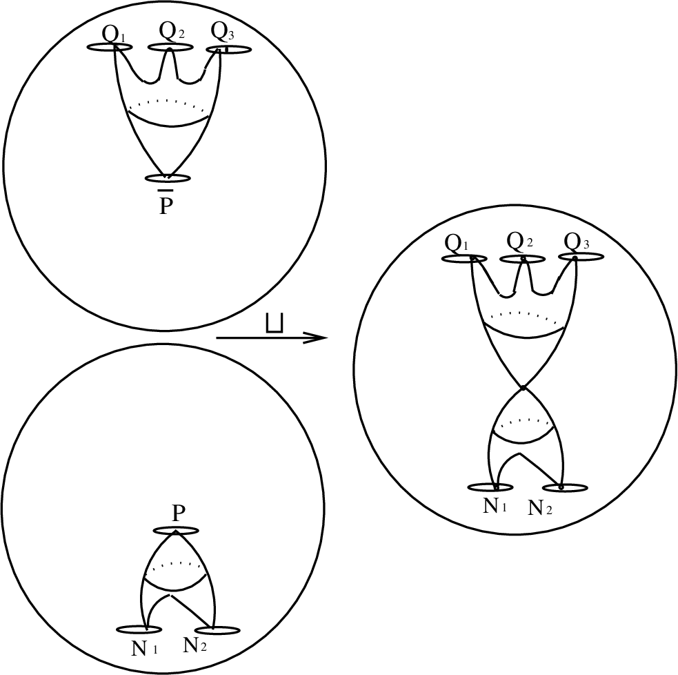
The map $a(\xi_{1},\cdots,\xi_{k})\colon K_{a}(\xi_{1},\cdots,\xi_{k})\times P_{1}\displaystyle\bigsqcup_{N_{1}}\cdots\displaystyle\bigsqcup_{N_{k-1}}P_{k}\to M$ is given by $a(\xi_{1},\cdots,\newline \xi_{k})((s,t_{1}\cdots,t_{k}),u)=\xi_{i}(t_{i})(u)$ for any tuple $(s,t_{1}\cdots,t_{k})$ in $K_{a}\times K_{\xi_{1}}\times_{\overline{N}_{1}}\cdots\times_{\overline{N}_{k-1}}K_{\xi_{k}}$ and $u\in P_{i}.$ Figure 4 represents a $n$-cobordism enriched over $M$ and Figure 4 shows a composition of $n$-cobordism enriches over $M.$

${\rm Cob}^{M}_{n,r}$ is the full subcategory of ${\rm Cob}^{M}_{n},$ such that the empty set is not included as an object.

Given monoidal categories ${\mathcal{C}}$ and ${\mathcal{D}}$ we denote by ${\rm MFunc}({\mathcal{C}},{\mathcal{D}})$ the category of monoidal functors from ${\mathcal{C}}$ to ${\mathcal{D}}.$

The map

is defined as follows: consider the natural projection $\pi\colon\displaystyle\prod_{i\in[n]}P\mid_{c(i)}\to\displaystyle\prod_{i\in[n]}c(i),$ and let $x$ be a chain $x\colon K_{x}\to\displaystyle\prod_{i\in[n]}P\mid_{c(i)},$ where $x=(x_{1},\dots,x_{n}).$ The domain of ${\rm H}_{\Lambda}(\alpha,t)(x)$ is given by

The map ${\rm H}_{\Lambda}(\alpha,t)(x)\colon K_{{\rm H}_{\Lambda}(\alpha,t)(x)}\to\displaystyle\prod_{i\in[n]}P\mid_{d(i)}$ is given by

where $y\in K_{x},\ y_{i}\in K_{t_{i}}.$

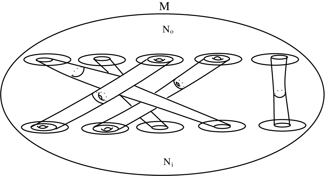
Fix a compact oriented manifold $M.$ We proceed to construct a higher dimensional homological analogue of matrices by generalizing the spaces $\textrm{Digraph}(m,n)$ as follows: 1) We replace each point of the set $[m]$ by oriented embedded submanifold of $M.$ So the indices of a generalized matrix are maps $c\colon[m]\to D(M).$ 2) The vector space $\textrm{Digraph}(m,n)$ is replaced by the space ${\rm HG}(c,d)$ of homological bipartite graphs with one packet of edges, where $c\colon[m]\to D(M)$ and $d\colon[n]\to D(M).$ The space ${\rm HG}(c,d)$ is given by

with degrees in ${\rm H}({\rm Map}(I,M)_{c(j),d(i)})$ shifted by $\dim(d(i)).$ 3) Given $A\in{\rm HG}(d,e)$ and $B\in{\rm HG}(c,d)$ then we define the product $AB\in{\rm HG}(c,e)$ of $A$ and $B$ by the rule

for all $i\in[n],j\in[m]\mbox{ and }k\in[p]$ where $B_{ji}\in{\rm H}({\rm Map}(I,M)_{c(i),d(j))},\ A_{kj}\in{\rm H}({\rm Map}(I,M)_{d(j),e(k))}$ and the composition maps

are defined as for $1$-dimensional homological quantum field theories.

For a map $c\colon[n]\to D(M),$ the space ${\rm HG}(c,c)$ is an algebra which may be regarded as higher dimensional homological analogue of $M_{n}(\mathbb{C}).$ A representation of ${\rm HG}(c,c)$ on a $\mathbb{C}$-vector space $V$ is a linear map $\rho\colon{\rm HG}(c,c)\to{{\rm End}}(V)$ such that $\rho(AB)=\rho(A)\rho(B).$ Figure 8 shows an example of product of homological matrix in ${\rm HG}(d,e)$ with a homological matrix ${\rm HG}(c,d).$

In [5] the $m$-symmetric power ${\rm S}^{m}{\rm A}$ of an algebra ${\rm A}$ is defined as follows: as a vector space ${\rm S}^{m}{\rm A}=({\rm A}^{\otimes m})_{S_{m}},$ ($S_{m}$-coinvariants.) The product in ${\rm S}^{m}{\rm A}$ is that as if $\overline{a_{1}\otimes\cdots\otimes a_{m}}\in{\rm S}^{m}{\rm A}$ and $\overline{b_{1}\otimes\cdots\otimes b_{m}}\in{\rm S}^{m}{\rm A}$ then

where ${\rm sgn}(a,b,\sigma)=(-1)^{e}$ and $e=e(a,b,\sigma)=\sum_{i>j}|a_{i}b_{\sigma^{-1}(j)}|+\sum_{\sigma(i)>\sigma(j)}|b_{i}b{{}_{j}}|.$

As shown in [5] if ${\rm A}$ is the algebra ${{\rm End}}({\mathbb{R}}^{p\mid q})$ of supermatrices of dimension $(p\mid q)\times(p\mid q)$ then ${\rm S}^{m}({{\rm End}})({\mathbb{R}}^{p\mid q})$ is the Schur superalgebra (see [7]) which controls the polynomial representations of ${{\rm End}}({\mathbb{R}}^{p\mid q}).$ We proceed to define Schur algebras in the homological context.

Figure 9 shows an element of ${\rm Schur}_{4}(c,c)={\rm S}^{4}({\rm H}(c,c)).$ Figure 10 shows a product in ${\rm Schur}_{2}(c,c).$

References

• [1] M. F. Atiyah, Topological quantum field theory I, Ann. Inst. Fourier (Grenoble) Publications mathématiques de l’Institut des Hautes Études Scientifiques, 17 (4), 1982, 661-692.
• [2] E. Castillo and R. Díaz, Homological quantum field theory , math.KT/0509532.
• [3] M. Chas and D. Sullivan,String Topology, Math.GT/9911159.
• [4] R. L.Cohen, and J. D. S. Jones, A homotopy theoretic realization of string topology, Math. Ann. 324 (4), 2002, 773-798.
• [5] R. Díaz and E. Pariguan. Quantum symmetric functions. Communications in Algebra. Vol 33, Issue 6, 2005, 1947-1978.
• [6] R. Diaz, and E. Pariguan, Graphical introduction to classical Lie algebras, math.RT/0504602. To appear in Boletin de la Asociacion Matemática Venezolana.
• [7] J. A. Green, Polynomial representations of G​LnGL_{n}, no. 830, Lecture notes in mathematics. Springer-Velarg, New York, 1980.
• [8] M. Karoubi, Cochaines quasi-commutatives en topologie algebrique, http://arxiv.org/ftp/math/papers/0509/0509268.pdf.
• [9] I. Kriz and J. P. May, Operads, Algebras, Modules, and Motives, 233, Astérisque, 1995.
• [10] R. Melrose, Differential analysis on manifolds with corners, http://www-math.mit.edu/ rbm/book.html.
• [11] G. B. Segal, The definition of conformal field theory, 1988.
• [12] D. Sullivan,Open and Closed String field theory interpreted in classical Algebraic Topology, Topology, Geometry and Quantum Field Theory. London Math. Soc. Lecture Notes vol. 308, (2004), 344-357.
• [13] R. Thom, Sur les variétés cobordantes., Colloque de topologie et géométrie différentielle, Strasbourg, 7, 1952, La Biblioth�ue Nationale et Universitaire de Strasbourg.
• [14] V. Turaev, Homotopy field theory in dimension 2 and group-algebras, QA/9910010.