跳到论文正文
W Papers独立论文阅读器 arXiv:math/0510260 论文正文 计算阅读时间 · 0%
引用这篇论文根据当前论文元数据生成,正式投稿前建议核对。


License: arXiv.org perpetual non-exclusive license
arXiv:math/0510260v4 [math.SG] 03 Apr 2009

A relative Seidel morphism and the Albers map

Shengda Hu Address: Department of pure mathematics, University of Waterloo, Waterloo (Ontario), Canada Current address: Email address: hshengda@math.uwaterloo.ca and François Lalonde Address: Département de mathématiques et de statistique, Université de Montréal, Montréal (Québec), Canada Current address: Email address: lalonde@dms.umontreal.ca
Abstract.

In this note, we introduce a relative (or Lagrangian) version of the Seidel homomorphism that assigns to each homotopy class of paths in Ham⁡(M){\rm Ham}(M), starting at the identity and ending on the subgroup that preserves a given Lagrangian submanifold LL, an element in the Floer homology of LL. We show that these elements are related to the absolute Seidel elements by the Albers map. We also study, for later use, the effect of reversing the signs of the symplectic structure as well as the orientations of the generators and of the operations on the Floer homologies.

2000 Mathematics Subject Classification
53D12, 53D40, 53D45, 57R58, 57S05

1. Introduction

Let (M,ω)(M,\omega) be a closed symplectic manifold. Seidel constructed in [16] a map from a covering of π1​Ham​(M,ω)\pi_{1}{\rm Ham}(M,\omega) to the invertible elements of either Q​H∗​(M,ω)QH_{*}(M,\omega) or F​H∗​(M)FH_{*}(M). It has found many uses, for example, in the study of Hamiltonian fibrations (Lalonde–McDuff–Polterovich [8]) and the quantum ring structure of toric varieties (McDuff-Tolman [11]). In this article, we introduce a similar construction when given a Lagrangian submanifold LL in (M,ω)(M,\omega). Instead of considering the loops in Ham⁡(M,ω){\rm Ham}(M,\omega), we consider the paths in Ham⁡(M,ω){\rm Ham}(M,\omega) starting at the identity and ending in the subgroup HamL​(M,ω){\rm Ham}_{L}(M,\omega):

HamL​(M,ω):={φ∈Ham⁡(M,ω)|φ⁡(L)=L}{\rm Ham}_{L}(M,\omega):=\{\varphi\in{\rm Ham}(M,\omega)|\varphi(L)=L\}

Another natural subgroup to consider consists of Hamiltonian symplectomorphisms that fix LL pointwisely. It is easy to see that any diffeomorphism of LL that is isotopic to the identity can be extended to a Hamiltonian symplectomorphism in MM that preserves LL. It follows that the two choices of subgroups essentially differ by Diff⁡(L){\rm Diff}(L). For the purpose of this paper, the reader can think of either choice.

Under the monotonicity assumption in the Lagrangian setting, one can define the Seidel elements for the elements in a covering of π1​(Ham⁡(M,ω),HamL​(M,ω))\pi_{1}({\rm Ham}(M,\omega),{\rm Ham}_{L}(M,\omega)). There is a homotopy exact sequence for the Hamiltonian groups, and we show that the following diagram commute (cf. corollary 3.16)

π~1​Ham​(M,ω)\textstyle{\widetilde{\pi}_{1}{\rm Ham}(M,\omega)\ignorespaces\ignorespaces\ignorespaces\ignorespaces\ignorespaces\ignorespaces\ignorespaces\ignorespaces}Ψ\scriptstyle{\Psi}π~1​(Ham⁡(M,ω),HamL​(M,ω))\textstyle{\widetilde{\pi}_{1}({\rm Ham}(M,\omega),{\rm Ham}_{L}(M,\omega))\ignorespaces\ignorespaces\ignorespaces\ignorespaces\ignorespaces\ignorespaces\ignorespaces\ignorespaces}ΨL\scriptstyle{\Psi_{L}}π~0​HamL​(M,ω)\textstyle{\widetilde{\pi}_{0}{\rm Ham}_{L}(M,\omega)}F​H∗​(M)\textstyle{FH_{*}(M)\ignorespaces\ignorespaces\ignorespaces\ignorespaces}𝒜\scriptstyle{\mathscr{A}}F​H∗​(M,L)\textstyle{FH_{*}(M,L)} (1.1)

where Ψ\Psi and ΨL\Psi_{L} denotes the respective absolute and relative Seidel maps and 𝒜\mathscr{A} denotes Albers’ comparison map between F​H∗​(M)FH_{*}(M) and F​H∗​(M,L)FH_{*}(M,L) [3].

We should explain the above diagram a little more. The Seidel maps are defined for the extensions π~1\widetilde{\pi}_{1} of the respective π1\pi_{1}’s by the corresponding period groups Γω\Gamma_{\omega} or ΓL\Gamma_{L}. An element g~∈π~1​Ham​(M,ω)\widetilde{g}\in\widetilde{\pi}_{1}{\rm Ham}(M,\omega) can be viewed canonically as an element in π~1​(Ham⁡(M,ω),HamL​(M,ω))\widetilde{\pi}_{1}({\rm Ham}(M,\omega),{\rm Ham}_{L}(M,\omega)) (cf. lemma 3.13) and the corresponding Seidel elements are related by 𝒜\mathscr{A}. The group π~0​HamL​(M,ω)\widetilde{\pi}_{0}{\rm Ham}_{L}(M,\omega) is an extension of π0​HamL​(M,ω)\pi_{0}{\rm Ham}_{L}(M,\omega) so that the top sequence is exact. On the other hand, we may adopt McDuff’s point of view in [10] where the Seidel map is defined on π1\pi_{1}’s directly by choosing a prefered extension g~\widetilde{g} for each g∈π1g\in\pi_{1}. Then (1.1) holds with the non-extended homotopy groups.

One of the original motivations for studying these Seidel elements and the above diagram was to obtain information on the third term in the exact sequence, namely π0​HamL​(M,ω)\pi_{0}{\rm Ham}_{L}(M,\omega). This is the most elementary question that one may ask about the subgroup HamL​(M,ω){\rm Ham}_{L}(M,\omega) of Hamiltonian transformations leaving a given Lagrangian submanifold invariant.

If, say, one calls the elements in the image of 𝒜∘Ψ{\mathscr{A}}\circ\Psi the circular Seidel elements in F​H∗​(M,L)FH_{*}(M,L) and the elements in the image of ΨL\Psi_{L} the semi-circular ones, then by the commutativity of the diagram, the latter ones contain the former ones. One could try to find semi-circular, but not circular, elements by computing explicitly the two Seidel morphisms. This would imply that

π1​Ham​(M,ω)→π1​(Ham⁡(M,ω),HamL​(M,ω))\pi_{1}{\rm Ham}(M,\omega)\rightarrow\pi_{1}({\rm Ham}(M,\omega),{\rm Ham}_{L}(M,\omega))

is not onto, and therefore π0​HamL​(M,ω)\pi_{0}{\rm Ham}_{L}(M,\omega) is not trivial. Of course, if a given component of HamL​(M,ω){\rm Ham}_{L}(M,\omega) is made of Hamiltonian diffeomorphisms whose restrictions to LL is not isotopic to the identity, it is obviously not the identity component. Hence our construction is useful when components are made of Hamiltonian diffeomorphisms whose restriction to LL is isotopic to the identity (or cannot be easily shown to be non-isotopic to the identity).

In presence of a real structure on MM, i.e. of an anti-symplectic involution cc with fixed point set LL, one could replace everywhere HamL​(M,ω){\rm Ham}_{L}(M,\omega) by its subgroup Hamc​(M,ω){\rm Ham}_{c}(M,\omega) of Hamiltonian diffeomorphisms of MM commuting with cc. Obviously the corresponding diagram (1.1) would still commute. In this paper, we restrict ourselves to a detailed setting of the theory, postponing to a forthcoming paper applications and computations of examples.

In section §2, we review Lagrangian Floer homology in the setting of Hamiltonian paths, cf. [3]. Other versions of Floer homology of a single Lagrangian already exist, e.g. [12, 4, 5, 6] by Oh, Fukaya–Oh–Ohta–Ono, Biran–Cornea. Because we will be working over ℝ{\mathbb{R}}, we include a discussion of the coherent orientation for the Floer trajectories, essentially following Fukaya–Oh–Ohta–Ono [6]. The necessary gluing is similar to those found in Albers [3]. The half-pair-of-pants product is analogous to the pair-of-pants product in the Hamiltonian Floer homology with some notorious differences (say its non-commutativity). It should coincide with the product defined from holomorphic triangles as in [6] or using the linear cluster complex as in [4]. For later use, we also discuss the action of F​H∗​(M)FH_{*}(M) as well as the Albers’ comparison map. Other versions of the action of F​H∗​(M)FH_{*}(M) has been described before, e.g. in the context of the linear cluster complex (or pearl complex) [4] or in the context of L∞L_{\infty}-action on the A∞A_{\infty}-algebra in [6].

In §3 we carry out Seidel’s construction for F​H∗​(M,L)FH_{*}(M,L) and show that it has the expected properties. It is also in this section that we show the commutativity of diagram (1.1). Finally, for later use related to the computations in (X,ω)×(X,−ω)(X,\omega)\times(X,-\omega), we explain in §4 and in §5 the effect of reversing the orientations of the generators of the symplectic and Lagrangian Floer homologies a well as the reversal of time in operations on Floer homologies.

We would like to mention here that the possibility of defining a relative Seidel morphism appears implicitly in the recent paper of Rémi Leclercq in [9]. Indeed, the proof of his basic proposition 3.1 that he needs to define his Lagrangian spectral invariants, contains the main ingredients of the construction of a relative Seidel morphism, even though it is not presented in these terms.

Acknowledgement. We would like to thank the referee for the constructive suggestions. The first author would like to thank Octav Cornea, Dusa McDuff and Jean-Yves Welschinger for valuable discussions.

2. Lagrangian Floer theory

Let (M,ω)(M,\omega) be a symplectic manifold and LL a Lagrangian submanifold. We set up here the Floer theory for (M,L)(M,L) with a generic Hamiltonian purturbation.

2.1. Novikov rings

We think of ω\omega, c1​(T​M)c_{1}(TM) and μL\mu_{L} as functions on π2​(M)\pi_{2}(M) or π2​(M,L)\pi_{2}(M,L) and denote them as:

Iω:π2​(M)​ or ​π2​(M,L)→ℝ,Ic:π2​(M)→ℝ​ and ​Iμ:π2​(M,L)→ℝ.I_{\omega}:\pi_{2}(M)\text{ or }\pi_{2}(M,L)\to{\mathbb{R}},I_{c}:\pi_{2}(M)\to{\mathbb{R}}\text{ and }I_{\mu}:\pi_{2}(M,L)\to{\mathbb{R}}.

Let

Γω=π2​(M)ker⁡Iω∩ker⁡Ic​ and ​ΓL=π2​(M,L)ker⁡Iω∩ker⁡Iμ,\Gamma_{\omega}=\frac{\pi_{2}(M)}{\ker I_{\omega}\cap\ker I_{c}}\text{ and }\Gamma_{L}=\frac{\pi_{2}(M,L)}{\ker I_{\omega}\cap\ker I_{\mu}},

where one could as well replace π2​(M)\pi_{2}(M) and π2​(M,L)\pi_{2}(M,L) by their images under the respective Hurewicz homomorphisms, namely, the spherical homology groups H2S​(M)H^{S}_{2}(M) and H2S​(M,L)H^{S}_{2}(M,L), since the quotients are the same11 1 If one adopts the point of view in [10] so that (1.1) holds for the non-extended groups, then the π2\pi_{2}’s are replaced by the respective the spherical homology in ℝ\mathbb{R}-coefficients, namely H2S​(M,ℝ)H^{S}_{2}(M;\mathbb{R}) and H2S​(M,L,ℝ)H^{S}_{2}(M,L;\mathbb{R}). The maps IωI_{\omega}, IcI_{c} and IμI_{\mu} are well defined on these homology groups and Γω\Gamma_{\omega} and ΓL\Gamma_{L} are defined as the respective quotients. . Then the Novikov rings for quantum (or Floer) homology are defined as follows:

Λω={∑B∈ΓωaBeB|aB∈ℝ and ∀K∈ℝ,#{B|aB≠0 and ω(B)<K}<∞}\Lambda_{\omega}=\left\{\left.\sum_{B\in\Gamma_{\omega}}a_{B}e^{B}\right|a_{B}\in{\mathbb{R}}\text{ and }\forall K\in{\mathbb{R}},\#\{B|a_{B}\neq 0\text{ and }\omega(B)<K\}<\infty\right\}
ΛL={∑B∈ΓLaBeB|aB∈ℝ and ∀K∈ℝ,#{B|aB≠0 and ω(B)<K}<∞}.\Lambda_{L}=\left\{\left.\sum_{B\in\Gamma_{L}}a_{B}e^{B}\right|a_{B}\in{\mathbb{R}}\text{ and }\forall K\in{\mathbb{R}},\#\{B|a_{B}\neq 0\text{ and }\omega(B)<K\}<\infty\right\}.

Their degrees are defined by deg⁡(eB)=−2​Ic​(B)\deg(e^{B})=-2I_{c}(B) and deg⁡(eB)=−Iμ​(B)\deg(e^{B})=-I_{\mu}(B). The homotopy exact sequence π2​(L)→π2​(M)→π2​(M,L)→π1​(L)\pi_{2}(L)\to\pi_{2}(M)\to\pi_{2}(M,L)\to\pi_{1}(L) induces an inclusion on the quotients

i:Γω→ΓL,i:\Gamma_{\omega}\to\Gamma_{L},

since ker⁡Iω∩ker⁡Ic\ker I_{\omega}\cap\ker I_{c} is mapped to ker⁡Iω∩ker⁡Iμ\ker I_{\omega}\cap\ker I_{\mu}. It follows that there is a natural inclusion of the Novikov rings:

i:Λω→ΛL.i:\Lambda_{\omega}\to\Lambda_{L}.

We can then make a ΛL\Lambda_{L}-module into a Λω\Lambda_{\omega}-module via this inclusion.

2.2. The flow equation

Let H:[0,1]×M→ℝH:[0,1]\times M\to{\mathbb{R}} be a time-dependent Hamiltonian function and 𝐉={Jt}t∈[0,1]\mathbf{J}=\{J_{t}\}_{t\in[0,1]} a time-dependent ω\omega-compatible almost complex structure. The space of such pairs is

ℋ​𝒥=C∞​([0,1]×M)×𝒥,\mathcal{HJ}=C^{\infty}([0,1]\times M)\times\mathcal{J},

where 𝒥\mathcal{J} is the space of one-parameter families of ω\omega-compatible almost complex structures. Let

D+2={z∈ℂ:|z|⩽1,ℑz⩾0},D^{2}_{+}=\{z\in{\mathbb{C}}:|z|{\leqslant}1,\Im z{\geqslant}0\},

∂+\partial_{+} denote the part of boundary of D+2D^{2}_{+} on the unit circle, parametrized by t∈[0,1]t\in[0,1] as ei​π​te^{i\pi t}, and ∂0\partial_{0} the part on the real line, parametrized by t∈[0,1]t\in[0,1] as 2​t−12t-1.

We consider the path space

𝒫LM={l:([0,1],{0,1})→(M,L)|[l]=0∈π1(M,L)}.{\mathcal{P}}_{L}M=\{l:([0,1],\{0,1\})\to(M,L)|[l]=0\in\pi_{1}(M,L)\}.

and the covering space 𝒫~L​M\widetilde{\mathcal{P}}_{L}M of 𝒫L​M{\mathcal{P}}_{L}M whose elements are the equivalence classes:

[l,w] where l∈𝒫LM and w:(D+2;∂+,∂0)→(M;l,L),[l,w]\text{ where }l\in{\mathcal{P}}_{L}M\text{ and }w:(D^{2}_{+};\partial_{+},\partial_{0})\to(M;l,L),

where

(l,w)∼(l′,w′)⇔l=l′​ and ​Iω​(w​#​(−w′))=Iμ​(w​#​(−w′))=0.(l,w)\sim(l^{\prime},w^{\prime})\iff l=l^{\prime}\text{ and }I_{\omega}(w\#(-w^{\prime}))=I_{\mu}(w\#(-w^{\prime}))=0.

The action functional on 𝒫~L​M\widetilde{\mathcal{P}}_{L}M is given by

aH([l,w])=−∫D+2w∗ω+∫[0,1]Ht(l(t))dt,a_{H}([l,w])=-\int_{D^{2}_{+}}w^{*}\omega+\int_{[0,1]}H_{t}(l(t))dt,

where we use the convention d​H=−ιXH​ωdH=-\iota_{X_{H}}\omega for the Hamiltonian vector fields. An element l~=[l,w]∈𝒫~L​M\widetilde{l}=[l,w]\in\widetilde{\mathcal{P}}_{L}M is a critical point of aHa_{H} if and only if ll is a Hamiltonian path connecting points on LL.

Definition 2.1.

A critical point l~\widetilde{l} is nondegenerate if d​ϕ1​Tl⁡(0)​L⋔Tl⁡(1)​Ld\phi_{1}T_{l(0)}L\pitchfork T_{l(1)}L, where ϕt∈[0,1]\phi_{t\in[0,1]} is the Hamiltonian isotopy generated by Ht∈[0,1]H_{t\in[0,1]}.

In a way similar to the case of Hamiltonian Floer homology on MM, we have

Proposition 2.2

For a generic HH, all critical points of aHa_{H} are non-degenerate. ∎

Floer theory studies the negative gradient flow of aHa_{H}. Let (,)𝐉(,)_{\mathbf{J}} be the metric on 𝒫L​M{\mathcal{P}}_{L}M defined by

(ξ,η)𝐉=∫[0,1]ω⁡(ξ⁡(t),Jt​η​(t))​𝑑t,(\xi,\eta)_{\mathbf{J}}=\int_{[0,1]}\omega(\xi(t),J_{t}\eta(t))dt,

then the equation of negative gradient flow for aHa_{H} is the following perturbed 𝐉\mathbf{J}-holomorphic equation for u:ℝ×[0,1]→Mu:{\mathbb{R}}\times[0,1]\to M:

{∂u∂s+Jt​(u)​(∂u∂t−XHt​(u))=0 for all ​(s,t)∈ℝ×[0,1],u|ℝ×{0,1}⊂L\left\{\begin{matrix}\frac{\partial u}{\partial s}+J_{t}(u)\left(\frac{\partial u}{\partial t}-X_{H_{t}}(u)\right)=0&\text{ for all }(s,t)\in{\mathbb{R}}\times[0,1],\\ u|_{{\mathbb{R}}\times\{0,1\}}\subset L\end{matrix}\right. (2.1)

The energy E⁡(u)E(u) of a solution uu of (2.1) with respect to the metric induced by 𝐉\mathbf{J} is defined as its ss-energy:

E⁡(u)=∫|∂u∂s|t2​𝑑s​𝑑tE(u)=\int\left|\frac{\partial u}{\partial s}\right|_{t}^{2}dsdt

where the tt-metric on MM is ⟨ξ,η⟩t=ω⁡(ξ,Jt​η){\langle}\xi,\eta{\rangle}_{t}=\omega(\xi,J_{t}\eta). Suppose that all critical points of aHa_{H} are non-degenerate, and let uu be a finite energy solution, then ls​(t):=u​(s,t)l_{s}(t):=u(s,t) converges uniformly to Hamiltonian paths in C0C^{0}-topology, i.e. ∃l±\exists l_{\pm} critical points of aHa_{H} so that lims→±∞ls​(t)=l±​(t)\lim_{s\to\pm\infty}l_{s}(t)=l_{\pm}(t) uniformly in tt.

2.3. Conley-Zehnder index

For each nondegenerate critical point l~=[l,w]\widetilde{l}=[l,w], we can define a Conley-Zehnder index μH​(l~)\mu_{H}(\widetilde{l}). Since D+2D^{2}_{+} is contractible, we find a symplectic trivialization Φ\Phi of the bundle w∗​T​Mw^{*}TM given by Φz:Tw⁡(z)​M→ℂn\Phi_{z}:T_{w(z)}M\to{\mathbb{C}}^{n} with standard symplectic structure ω0\omega_{0} on ℂn{\mathbb{C}}^{n}. We require that Φr​(Tw⁡(r)​L)=ℝn\Phi_{r}(T_{w(r)}L)={\mathbb{R}}^{n} for r∈∂0D+2⊂D+2r\in\partial_{0}D^{2}_{+}\subset D^{2}_{+}, which is possible since ∂0D+2\partial_{0}D^{2}_{+} is contractible. Then the linearized Hamiltonian flow d​ϕtd\phi_{t} along ll defines a path of symplectic matrices

Et=Φei​π​t∘d​ϕt∘Φ1−1∈S​p​(ℂn).E_{t}=\Phi_{e^{i\pi t}}\circ d\phi_{t}\circ\Phi^{-1}_{1}\in Sp({\mathbb{C}}^{n}).

The Conley-Zehnder index of l~\widetilde{l} is defined using the Maslov index of paths of Lagrangian subspaces introduced in Robbin-Salamon [14]:

Proposition (Definition) 2.3

The Conley-Zehnder index of l~\widetilde{l} is defined as μH​(l~)=μ⁡(Et​ℝn,ℝn)\mu_{H}(\widetilde{l})=\mu(E_{t}{\mathbb{R}}^{n},{\mathbb{R}}^{n}); it satisfies:

  1. (1)

    μH​(l~)\mu_{H}(\widetilde{l}) does not depend on the trivialization;

  2. (2)

    μH​(l~)+n2∈ℤ\mu_{H}(\widetilde{l})+\frac{n}{2}\in{\mathbb{Z}};

  3. (3)

    under the deck transformation by β∈ΓL\beta\in\Gamma_{L}, we have μH​(l~​#​β)=μH​(l~)+Iμ​(β)\mu_{H}(\widetilde{l}\#\beta)=\mu_{H}(\widetilde{l})+I_{\mu}(\beta).

Proof.

For (2)(2) see [14], Theorem 2.42.4. The rest can be shown similarly as in the case of Hamiltonian loops in MM. ∎

Definition 2.4.

The Floer chain group is FC∗(H)=⊕kFCk(H)FC_{*}(H)=\oplus_{k}FC_{k}(H) where

FCk(H):={∑μH​(l~)=kal~l~|al~∈ℝ and ∀K∈ℝ,#{l~|al~≠0,aH(l~)<K}<∞}.FC_{k}(H):=\left\{\left.\sum_{\mu_{H}(\widetilde{l})=k}a_{\widetilde{l}}\widetilde{l}\right|a_{\tilde{l}}\in{\mathbb{R}}\text{ and }\forall K\in{\mathbb{R}},\#\{\widetilde{l}|a_{\widetilde{l}}\neq 0,a_{H}(\widetilde{l})<K\}<\infty\right\}.

It is easy to see that F​C∗​(H)FC_{*}(H) is a graded module over the Novikov ring ΛL\Lambda_{L} via:

eB⋅l~=l~​#​βe^{B}\cdot\widetilde{l}=\widetilde{l}\#\beta

and we have

eB⋅F​C∗​(H)⊂F​C∗−deg⁡(eB)​(H).e^{B}\cdot FC_{*}(H)\subset FC_{*-\deg(e^{B})}(H).

We note that by the ring inclusion i:Λω→ΛLi:\Lambda_{\omega}\to\Lambda_{L}, F​C∗​(H)FC_{*}(H) is also a Λω\Lambda_{\omega}-module.

2.4. The linearized operator and moduli spaces of flows

Let us suppose that all critical points of aHa_{H} are non-degenerate and consider the linearized operator of (2.1) at a finite energy solution uu

Du​ξ=∇∂∂sξ+Jt​(u)​∇∂∂tξ+∇ξJt​(u)​∂tu−∇ξ(Jt​(u)​XHt​(u)),D_{u}\xi=\nabla_{\frac{\partial}{\partial s}}\xi+J_{t}(u)\nabla_{\frac{\partial}{\partial t}}\xi+\nabla_{\xi}J_{t}(u)\partial_{t}u-\nabla_{\xi}\left(J_{t}(u)X_{H_{t}}(u)\right), (2.2)

where ξ∈Γ⁡(u∗​T​M,L)={ξ∈Γ⁡(u∗​T​M)|ξ|ℝ×{0,1}⊂T​L}\xi\in\Gamma(u^{*}TM;L)=\{\xi\in\Gamma(u^{*}TM)|\xi|_{{\mathbb{R}}\times\{0,1\}}\subset TL\}. Under suitable Banach completion, Du:Lkp​(u∗​T​M,L)→Lk−1p​(u∗​T​M)D_{u}:L^{p}_{k}(u^{*}TM;L)\to L^{p}_{k-1}(u^{*}TM) is Fredholm whose index is the expected dimension of the space of solutions near uu.

By [15] (Theorem 7.1), the index can be identified as the difference of the Conley-Zehnder indices of the two ends:

Proposition 2.5

Let ℳ~H,𝐉​(M,L,l~−,l~+)\widetilde{{\mathcal{M}}}_{H,\mathbf{J}}(M,L;\widetilde{l}_{-},\widetilde{l}_{+}) be the space of all solutions of the equation (2.1) connecting l~−\widetilde{l}_{-} to l~+\widetilde{l}_{+} such that [l~−​#​u​#​(−l~+)]=0∈ΓL[\widetilde{l}_{-}\#u\#(-\widetilde{l}_{+})]=0\in\Gamma_{L}. Its expected dimension is then given by:

ind​Du=μH​(l~−)−μH​(l~+).{\rm ind}D_{u}=\mu_{H}(\widetilde{l}_{-})-\mu_{H}(\widetilde{l}_{+}).

∎

The unparametrized moduli space is ℳH,𝐉​(M,L,l~−,l~+)=ℳ~H,𝐉​(M,L,l~−,l~+)/ℝ{\mathcal{M}}_{H,\mathbf{J}}(M,L;\widetilde{l}_{-},\widetilde{l}_{+})=\widetilde{{\mathcal{M}}}_{H,\mathbf{J}}(M,L;\widetilde{l}_{-},\widetilde{l}_{+})/{\mathbb{R}} where the ℝ{\mathbb{R}} action is the shifting of ss. Thus we have in generic conditions:

dimℳH,𝐉​(M,L,l~−,l~+)=μH​(l~−)−μH​(l~+)−1.\dim{\mathcal{M}}_{H,\mathbf{J}}(M,L;\widetilde{l}_{-},\widetilde{l}_{+})=\mu_{H}(\widetilde{l}_{-})-\mu_{H}(\widetilde{l}_{+})-1.

2.5. Coherent orientations

We will work over ℚ{\mathbb{Q}} or ℂ{\mathbb{C}} instead of ℤ2{\mathbb{Z}}_{2}. For this reason, we impose the following assumption from now on:

Assumption 2.6.

LL is relatively spin, i.e. LL is orientable and w2​(L)∈H2​(L,ℤ2)w_{2}(L)\in H^{2}(L;{\mathbb{Z}}_{2}) extends to a class in H2​(M)H^{2}(M).

The above assumption implies that the moduli spaces of holomorphic discs with boundary on LL can be canonically oriented with the choice of a relatively spin structure on LL, i.e.

  • •

    an orientation of LL,

  • •

    an extension of w2​(L)w_{2}(L) to H2​(M)H^{2}(M) and

  • •

    a spin structure on T​L⊕V|L(2)TL\oplus V|_{L_{(2)}}, i.e. a trivialization of T​L⊕V|L(1)TL\oplus V|_{L_{(1)}} that extends to L(2)L_{(2)},

where L(2)L_{(2)} is the 22-skeleton of some triangulation of LL and VV is an oriented real vector bundle on the 33-skeleton M(3)M_{(3)} of MM so that w2​(V)w_{2}(V) extends w2​(L)w_{2}(L). It follows that T​L⊕V|L(2)TL\oplus V|_{L_{(2)}} is indeed spin. Starting from these choices, we may assign to the moduli spaces ℳ~H,𝐉​(M,L,l~−,l~+)\widetilde{\mathcal{M}}_{H,\mathbf{J}}(M,L;\widetilde{l}_{-},\widetilde{l}_{+}) a coherent orientation (see for example [6], §4444) in the following way.

First, in order to orient the moduli space of half-tubes ℳ~H,𝐉​(M,L,l~−,l~+)\widetilde{\mathcal{M}}_{H,\mathbf{J}}(M,L;\widetilde{l}_{-},\widetilde{l}_{+}), we consider essentially an oriented version of the argument for the PSS [3]. It involves another type of moduli spaces ℳ~H±,𝐉±±​(M,L,l~)\widetilde{\mathcal{M}}^{\pm}_{H^{\pm},\mathbf{J}^{\pm}}(M,L;\widetilde{l}) consisting of maps from either the capped strip Z−Z_{-} or Z+Z_{+} ([3]):

ℂ⊃Z±=D∓2∪(ℝ±×[0,1])→u±M​ so that ​u​(∂Z±)⊂L.{\mathbb{C}}\supset Z_{\pm}=D^{2}_{\mp}\cup({\mathbb{R}}^{\pm}\times[0,1])\xrightarrow{u^{\pm}}M\text{ so that }u({\partial Z_{\pm}})\subset L. (2.3)

where this time D−2D^{2}_{-} denotes the closed left half part of the disk of raduis 1/21/2 centered at 1/2​i∈ℂ1/2i\in{\mathbb{C}} while D+2D^{2}_{+} denotes the closed right half part. The coordinates in Z±Z_{\pm} is z=s+i​tz=s+it. Choose and fix (H±,𝐉±)(H^{\pm},\mathbf{J}^{\pm}), a pair of smoothly zz-dependent Hamiltonian function and almost complex structures so that

(H±,𝐉±)|D∓2=(0,J)​ and ​(H±,𝐉±)|1∓s<0=(H,𝐉),(H^{\pm},\mathbf{J}^{\pm})|_{D^{2}_{\mp}}=(0,J)\text{ and }(H^{\pm},\mathbf{J}^{\pm})|_{1\mp s<0}=(H,\mathbf{J}),

where JJ is a generic almost complex structure on MM. Consider the equation for u±:Z±→Mu^{\pm}:Z_{\pm}\to M:

{∂u±∂s+Jz±​(u±)​(∂u±∂t−XHz±​(u±))=0 for all ​(s,t)∈Z±,u|∂Z±⊂L\left\{\begin{matrix}\frac{\partial u^{\pm}}{\partial s}+J^{\pm}_{z}(u^{\pm})\left(\frac{\partial u^{\pm}}{\partial t}-X_{H^{\pm}_{z}}(u^{\pm})\right)=0&\text{ for all }(s,t)\in Z_{\pm},\\ u|_{\partial Z_{\pm}}\subset L\end{matrix}\right. (2.4)

The energy E⁡(u±)E(u^{\pm}) is defined as the ss-energy in the usual way, and finite energy solutions u±u^{\pm} converge uniformly to Hamiltonian paths of HH when s→±∞s\to\pm\infty. Then set

ℳ~H±,𝐉±(M,L;l~):={u±:Z±→M|u±​ satisfies (2.4),lims→±∞u±=l​ and [l~​#​(−u±)]=0∈ΓL}.\widetilde{\mathcal{M}}_{H^{\pm},\mathbf{J}^{\pm}}(M,L;\widetilde{l}):=\left\{u^{\pm}:Z_{\pm}\to M\left|\begin{matrix}u^{\pm}\text{ satisfies \eqref{lagFloer:capeq}},\\ \lim_{s\to\pm\infty}u^{\pm}=l\text{ and }\\ [\widetilde{l}\#(-u^{\pm})]=0\in\Gamma_{L}\end{matrix}\right.\right\}.

There are evaluation maps for these moduli spaces, at the points p±=±1/2+1/2i∈D2±p_{\pm}=\pm 1/2+1/2i\in D^{2}_{\pm}:

e​v±:ℳ~H±,𝐉±​(M,L,l~)→L:u±↦u±​(p∓).ev^{\pm}:\widetilde{\mathcal{M}}_{H^{\pm},\mathbf{J}^{\pm}}(M,L;\widetilde{l})\to L:u^{\pm}\mapsto u^{\pm}(p_{\mp}).

We argue that a choice of the orientations of all the moduli spaces of the form ℳ~H+,𝐉+​(M,L,l~+)\widetilde{\mathcal{M}}_{H^{+},\mathbf{J}^{+}}(M,L;\widetilde{l}^{+}) induces the orientations of the moduli spaces of the form ℳ~H−,𝐉−​(M,L,l~−)\widetilde{\mathcal{M}}_{H^{-},\mathbf{J}^{-}}(M,L;\widetilde{l}^{-}) where l+=l−l^{+}=l^{-}. We consider the gluing of the equations (2.4) for the moduli spaces ℳ~H+,𝐉+​(M,L,l~+)\widetilde{\mathcal{M}}_{H^{+},\mathbf{J}^{+}}(M,L;\widetilde{l}^{+}) and ℳ~H−,𝐉−​(M,L,l~−)\widetilde{\mathcal{M}}_{H^{-},\mathbf{J}^{-}}(M,L;\widetilde{l}^{-}) along ll. That is, choose and fix an appropriate cut off function β\beta and consider the domains

Z+,R=D−2∪([0,R+1]×[0,1])​ and ​Z−,R=D+2∪([−R−1,0]×[0,1]),Z_{+,R}=D^{2}_{-}\cup([0,R+1]\times[0,1])\text{ and }Z_{-,R}=D^{2}_{+}\cup([-R-1,0]\times[0,1]),

and use β\beta to glue the two equations on Z±Z_{\pm} to define an equation on the glued domain

ZR:=Z+,R⊔Z−,R/(z∼z−R−1​ in the ends).Z_{R}:=Z_{+,R}\sqcup Z_{-,R}/(z\sim z-R-1\text{ in the ends}).

We note that ZRZ_{R} is conformal to D2D^{2} and the equation on ZRZ_{R} is in fact a compact perturbation of the ∂¯J\bar{\partial}_{J}-equation for discs with boundary on LL. Because the moduli space of discs is canonically oriented by the choice of a relatively spin structure, we see that the moduli space ℳ~H±,𝐉±​(M,L,l~,R)\widetilde{\mathcal{M}}_{H^{\pm},\mathbf{J}^{\pm}}(M,L;\widetilde{l},R) for the glued equation on ZRZ_{R} is oriented. From the additivity of indices by standard gluing arguments, we see that the orientations of the ++-moduli spaces induce orientations of the −--moduli spaces.

Let B∈π2​(M,L)B\in\pi_{2}(M,L) and consider l~B=l~​#​B\widetilde{l}^{B}=\widetilde{l}\#B. When ℳ~H+,𝐉+​(M,L,l~B)\widetilde{\mathcal{M}}_{H^{+},\mathbf{J}^{+}}(M,L;\widetilde{l}^{B}) is not empty, its orientation is defined from that of ℳ~H+,𝐉+​(M,L,l~)\widetilde{\mathcal{M}}_{H^{+},\mathbf{J}^{+}}(M,L;\widetilde{l}) and the ∂¯\bar{\partial}-equation for discs with boundary on LL representing class BB. We note that the moduli space of discs might be empty, or the ∂¯\bar{\partial}-operator might be non-surjective. Nevertheless, an orientation can be assigned to the index of the ∂¯\bar{\partial}-operator. Summarizing, we have

Proposition 2.7

The orientations of the moduli spaces ℳ~H±,𝐉±​(M,L,l~)\widetilde{\mathcal{M}}_{H^{\pm},\mathbf{J}^{\pm}}(M,L;\widetilde{l}) are determined by the canonical orientations on the indices of the ∂¯\bar{\partial}-operators of discs with boundaries on LL as well as a choice of the orientations on ℳ~H+,𝐉+​(M,L,l~j)\widetilde{\mathcal{M}}_{H^{+},\mathbf{J}^{+}}(M,L;\widetilde{l}_{j}) for a ΛL\Lambda_{L}-basis {l~j}\{\widetilde{l}_{j}\} of F​C∗​(H)FC_{*}(H). ∎

Definition 2.8.

The basis {l~j}\{\widetilde{l}_{j}\} is called a preferred basis for the orientation of the Floer complex F​C∗​(M,L,H,𝐉)FC_{*}(M,L;H,\mathbf{J}).

To obtain the orientations for the moduli spaces ℳ~H,𝐉​(M,L,l~−,l~+)\widetilde{\mathcal{M}}_{H,\mathbf{J}}(M,L;\widetilde{l}_{-},\widetilde{l}_{+}), we notice, for example, that gluing these latter moduli spaces with the moduli spaces ℳ~H+,𝐉+​(M,L,l~−)\widetilde{\mathcal{M}}_{H^{+},\mathbf{J}^{+}}(M,L;\widetilde{l}_{-}) yields the moduli spaces ℳ~H+,𝐉+​(M,L,l~+)\widetilde{\mathcal{M}}_{H^{+},\mathbf{J}^{+}}(M,L;\widetilde{l}_{+}). Since both the latter two have been given orientations, these orientations canonically determine orientations on the moduli spaces of half-tubes. Considering the opposite gluing, that is to say using ℳ~H−,𝐉−​(M,L,l~+)\widetilde{\mathcal{M}}_{H^{-},\mathbf{J}^{-}}(M,L;\widetilde{l}_{+}) instead of ℳ~H+,𝐉+​(M,L,l~−)\widetilde{\mathcal{M}}_{H^{+},\mathbf{J}^{+}}(M,L;\widetilde{l}_{-}), would give the same induced orientations. It is now easy to see that the orientations introduced on ℳ~H,𝐉​(M,L,l~−,l~+)\widetilde{\mathcal{M}}_{H,\mathbf{J}}(M,L;\widetilde{l}_{-},\widetilde{l}_{+}) are naturally coherent in the sense of Hofer-Salamon [7].

2.6. Floer homology

From now on, we consider only monotone Lagrangians, i.e. satisfies the following:

 there is ​λ>0​ such that ​Iω=λ​Iμ​ on ​π2​(M,L).\text{ there is }\lambda>0\text{ such that }I_{\omega}=\lambda I_{\mu}\text{ on }\pi_{2}(M,L). (2.5)

Together with assumption 2.6, we see that the minimal Maslov number of LL is at least 22. The monotonicity condition also ensures that there are no non-trivial holomorphic spheres with non-positive Chern numbers or non-trivial discs with boundary on LL with non-positive Maslov index.

Let Mk​(𝐉)M_{k}(\mathbf{J}) denote the set of points of MM lying on non-constant JJ-holomorphic spheres with Chern number ⩽k\leqslant k, Lk​(𝐉)L_{k}(\mathbf{J}) the set of points of LL lying on the boundary of non-constant JJ-holomorphic discs with Maslov number ⩽k\leqslant k and P⁡(H)P(H) be the set of points of MM lying on connecting orbits of HH. In the following, we will assume that the pair (H,𝐉)(H,\mathbf{J}) is regular in the sense that

  • •

    all J0/1J_{0/1}-holomorphic discs with Maslov index 22 are regular,

  • •

    𝐉\mathbf{J} is regular for pseudo-holomorphic spheres with Chern number 11,

  • •

    all connecting orbits of HH are non-degenerate,

  • •

    DuD_{u} is surjective for finite energy solutions uu of (2.1) with index ​Du⩽2\text{index }D_{u}\leqslant 2.

  • •

    P⁡(H)∩M1​(𝐉)=∅P(H)\cap M_{1}(\mathbf{J})=\emptyset and P​(H)∩L2​(𝐉)P(H)\cap L_{2}(\mathbf{J}) is empty or of dimension 00.

Standard arguments (cf. e.g. [7]) implies that generic pairs are regular.

The Floer chain complex F​C∗​(H,𝐉)FC_{*}(H,\mathbf{J}) is given by the Floer chain group F​C∗​(H)FC_{*}(H) with the boundary map defined from counting the 00-dimensional moduli space of solutions:

∂H,𝐉l~−=∑μH​(l~−)=μH​(l~+)+1#​ℳH,𝐉​(M,L,l~−,l~+)​l~+,\partial_{H,\mathbf{J}}\widetilde{l}_{-}=\sum_{\mu_{H}(\widetilde{l}_{-})=\mu_{H}(\widetilde{l}_{+})+1}\#{\mathcal{M}}_{H,\mathbf{J}}(M,L;\widetilde{l}_{-},\widetilde{l}_{+})\widetilde{l}_{+},

and extending linearly. We then show that

Proposition 2.9

With assumptions 2.6 and assume that (H,𝐉)(H,\mathbf{J}) is regular, then ∂H,𝐉2=0\partial_{H,\mathbf{J}}^{2}=0.

Proof: Writing

∂H,𝐉2l~−=∑μH​(l~−)=μH​(l~0)+1#​ℳH,𝐉​(M,L,l~−,l~0)​∑μH​(l~0)=μH​(l~+)+1#​ℳH,𝐉​(M,L,l~0,l~+)​l~+\partial_{H,\mathbf{J}}^{2}\widetilde{l}_{-}=\sum_{\mu_{H}(\widetilde{l}_{-})=\mu_{H}(\widetilde{l}_{0})+1}\#{\mathcal{M}}_{H,\mathbf{J}}(M,L;\widetilde{l}_{-},\widetilde{l}_{0})\sum_{\mu_{H}(\widetilde{l}_{0})=\mu_{H}(\widetilde{l}_{+})+1}\#{\mathcal{M}}_{H,\mathbf{J}}(M,L;\widetilde{l}_{0},\widetilde{l}_{+})\widetilde{l}_{+}

we see that the proposition is equivalent to saying that for each pair of l~−\widetilde{l}_{-} and l~+\widetilde{l}_{+}, we have

∑μH​(l~−)=μH​(l~0)+1∑μH​(l~0)=μH​(l~+)+1#​ℳH,𝐉​(M,L,l~0,l~+)​#​ℳH,𝐉​(M,L,l~−,l~0)=0.\sum_{\mu_{H}(\widetilde{l}_{-})=\mu_{H}(\widetilde{l}_{0})+1}\sum_{\mu_{H}(\widetilde{l}_{0})=\mu_{H}(\widetilde{l}_{+})+1}\#{\mathcal{M}}_{H,\mathbf{J}}(M,L;\widetilde{l}_{0},\widetilde{l}_{+})\#{\mathcal{M}}_{H,\mathbf{J}}(M,L;\widetilde{l}_{-},\widetilde{l}_{0})=0.

The summand above is the counting for the moduli space of the broken half-tubes connecting l~±\widetilde{l}_{\pm}. The moduli space of broken half-tubes is part of the boundary components of the 11-dimensional moduli space ℳH,𝐉​(M,L,l~−,l~+){\mathcal{M}}_{H,\mathbf{J}}(M,L;\widetilde{l}_{-},\widetilde{l}_{+}).

Let 𝒞\mathcal{C} be a connected component of the (compactification) of ℳH,𝐉​(M,L,l~−,l~+){\mathcal{M}}_{H,\mathbf{J}}(M,L;\widetilde{l}_{-},\widetilde{l}_{+}). A boundary point of 𝒞\mathcal{C} is of type II if it is a broken half-tube, is type I​III if it is a bubbling off of holomorphic discs. The counting in ∂H,𝐉2\partial^{2}_{H,\mathbf{J}} concerns the type II boundaries. We have the following 33 cases for ∂𝒞\partial\mathcal{C}:

  • •

    empty or is of type I​III on both ends, or

  • •

    is of type II on both ends, or

  • •

    is of type II on one end and type I​III on the other.

Obviously, if no type I​III boundary occur in the compactification, an argument similar to the Hamiltonian Floer theory gives the proposition. In the following, we assume that type I​III boundary does occur. Then the type II boundary and type I​III boundary are cobordant and the vanishing of counting for either type implies the vanishing of the other. In the following we show the vanishing of counting for the type I​III boundary points, which would then imply the proposition.

Assume that type I​III boundary does occur. Then there exist critical points l~±\widetilde{l}_{\pm} and a holomorphic disc vv with μL=2\mu_{L}=2 so that vv is attached to a solution uu of (2.1) such that lims→±∞u⁡(s,t)=l±\lim_{s\to\pm\infty}u(s,t)=l_{\pm}. It follows that μH​(l~−)=μH​(l~+)\mu_{H}(\widetilde{l}_{-})=\mu_{H}(\widetilde{l}_{+}). By regularity assumptions, we see that l~−=l~+=l~\widetilde{l}_{-}=\widetilde{l}_{+}=\widetilde{l} where ll is a connecting Hamiltonian orbit of HH and u⁡(s,t)=l⁡(t)u(s,t)=l(t) for all ss. Also by our assumption, L2​(𝐉)L_{2}(\mathbf{J}) is compact of dimension nn. It follows that there are J0/1J_{0/1}-holomorphic discs through each point of LL.

The orientations of the moduli spaces of J0/1J_{0/1}-holomorphic discs with minimal Maslov number are consistent in the sense that they are connected through cobordisms. On the other hand, the orientation of ℳH,𝐉​(M,L,l~−,l~+)≠∅{\mathcal{M}}_{H,\mathbf{J}}(M,L;\widetilde{l}_{-},\widetilde{l}_{+})\neq\emptyset is obtained as in §2.5, by considering the gluing operations, via the canonical orientation of the moduli space of disc together with the choice of orientations on the moduli spaces ℳ~+\widetilde{\mathcal{M}}_{+}. The boundary components of ℳH,𝐉​(M,L,l~−,l~+){\mathcal{M}}_{H,\mathbf{J}}(M,L;\widetilde{l}_{-},\widetilde{l}_{+}) is oriented by considering the gluing operations. To derive the orientation of the type I​III boundary points, we need to consider the gluing of the following moduli spaces to the main component ll:

the moduli spaces ℳ~±\widetilde{\mathcal{M}}_{\pm} of the capped strips and the moduli space ℳ1​(M,L,B,J0/1){\mathcal{M}}_{1}(M,L;B,J_{0/1}) of 11-marked J0/1J_{0/1}-holomorphic disc with μL​(B)=2\mu_{L}(B)=2.

The ordering of the gluing operations is given by the orientation of the half-tube ℝ×[0,1]{\mathbb{R}}\times[0,1]. Namely, for the case of bubbling off of a disc at t=0t=0, the cyclic order is ℳ~+\widetilde{\mathcal{M}}_{+}, ℳ1​(M,L,B,J0){\mathcal{M}}_{1}(M,L;B,J_{0}) then ℳ~−\widetilde{\mathcal{M}}_{-} and for bubbling off at t=1t=1, the order is ℳ~−\widetilde{\mathcal{M}}_{-}, ℳ1​(M,L,B,J1){\mathcal{M}}_{1}(M,L;B,J_{1}) then ℳ~+\widetilde{\mathcal{M}}_{+}. Note that the orientations of the moduli spaces of holomorphic discs are consistent, while the cyclic ordering of the gluing operations are opposite. It follows that the counting of configuration of bubbling off at t=0t=0 and t=1t=1 have opposite signs. It then follows that the counting of type I​III boundary points vanishes, which implies ∂H,𝐉2=0\partial_{H,\mathbf{J}}^{2}=0. ∎

Thus we define the Floer homology of (M,L)(M,L) for the regular pair (H,𝐉)(H,\mathbf{J}) to be

FH∗(M,L;H,𝐉)=H∗(FC∗(H,𝐉),∂H,𝐉).FH_{*}(M,L;H,\mathbf{J})=H_{*}(FC_{*}(H,\mathbf{J}),\partial_{H,\mathbf{J}}).

The independence of F​H∗​(M,L,H,𝐉)FH_{*}(M,L;H,\mathbf{J}) with respect to the choices of (regular) HH and 𝐉\mathbf{J} can be seen using the usual arguments of continuation principle and homotopy of homotopies.

2.7. Half pair of pants product

The product on F​H∗​(M,L)FH_{*}(M,L) can be defined by “half pair-of-pants”, perturbed similarly as in Seidel [16], as following. Consider the half cylinder with a boundary puncture Σ0=ℝ×[0,1]∖{(r,0)}\Sigma_{0}={\mathbb{R}}\times[0,1]\setminus\{(r,0)\}. The surface Σ0\Sigma_{0} has three ends e±e_{\pm} and e0e_{0}:

e+:[1,∞)×[0,1]→Σ0 and e−:(−∞,−1]×[0,1]→Σ0e_{+}:[1,\infty)\times[0,1]\to\Sigma_{0}\text{ and }e_{-}:(-\infty,-1]\times[0,1]\to\Sigma_{0}

where e±​(s,t)=(s,t)e_{\pm}(s,t)=(s,t), and

e0:(−∞,−1]×[0,1]→Σ0:(b,θ)↦s+it=eb−1+π​i​θe_{0}:(-\infty,-1]\times[0,1]\to\Sigma_{0}:(b,\theta)\mapsto s+it=e^{b-1+\pi i\theta}

is holomorphic with respect to the standard complex structures on the domain and target, whose image lies completely in (−12,12)×(0,14)(-\frac{1}{2},\frac{1}{2})\times(0,\frac{1}{4}). The ends e−e_{-} and e0e_{0} are the “incoming” ends and e+e_{+} is the “outgoing end”. We choose regular pairs (H±,𝐉±)(H_{\pm},\mathbf{J}_{\pm}) and (H0,𝐉0)(H_{0},\mathbf{J}_{0}) for the corresponding ends. Consider the pair (𝐇,𝐉)(\mathbf{H},\mathbf{J}) where 𝐇∈C∞​(Σ×M)\mathbf{H}\in C^{\infty}(\Sigma\times M) and 𝐉\mathbf{J} is a family of compatible almost complex structures parametrized by Σ\Sigma, such that the pull back of (𝐇,𝐉)(\mathbf{H},\mathbf{J}) by the maps e∗e_{*} is equal to the corresponding pair (H∗,𝐉∗)(H_{*},\mathbf{J}_{*}). Furthermore, we require that 𝐇\mathbf{H} restricts to 00 over e0​([−2,−1]×[0,1])×Me_{0}([-2,-1]\times[0,1])\times M.

Remark 2.10.

Here and in the following, a region 𝒟⊂ℝ×[0,1]\mathscr{D}\subset{\mathbb{R}}\times[0,1] is provided with cylindrical coordinates if there is a biholomorphic map e:I×S→𝒟e:I\times S\to\mathscr{D} where I⊂ℝI\subset{\mathbb{R}} is a (possibly infinite) interval and S=[0,1]S=[0,1] or ℝ/ℤ{\mathbb{R}}/{\mathbb{Z}}. When we ask for the regular pair (𝐇,𝐉)(\mathbf{H},\mathbf{J}) to pull back to a pair (H′,𝐉′)(H^{\prime},\mathbf{J}^{\prime}) on a region provided with cylindrical coordinates I×SI\times S, we mean that there is a sequence of (nonempty) smaller intervals

I′′⊂I′′¯⊊(I′)∘⊂I′¯⊊I∘⊂I,I^{\prime\prime}\subset\bar{I^{\prime\prime}}\subsetneq(I^{\prime})^{\circ}\subset\bar{I^{\prime}}\subsetneq I^{\circ}\subset I,

so that (𝐇,𝐉)(\mathbf{H},\mathbf{J}) pull-backs to (H′,𝐉′)(H^{\prime},\mathbf{J}^{\prime}) on e⁡(I′′×S)e(I^{\prime\prime}\times S) while it pulls-back to (0,J0)(0,J_{0}) on e⁡((I∖I′)×S)e((I\setminus I^{\prime})\times S) for some fixed generic compatible almost complex structure J0J_{0}.

The description is conveniently summarized on figure 1.

Refer to caption
Figure 1.

Let (ℝ×[0,1])0=(ℝ×[0,1])∖e0((−∞,−1]×[0,1])({\mathbb{R}}\times[0,1])^{0}=({\mathbb{R}}\times[0,1])\setminus e_{0}((-\infty,-1]\times[0,1]) and consider the equation

{∂u∂s+Js,t​(u)​(∂u∂t−XHs,t​(u))=0 for ​(s,t)∈(ℝ×[0,1])0,∂u0∂s+Je0​(s,t)​(u0)​(∂u0∂t−XHe0​(s,t)​(u0))=0 for (s,t)∈(−∞,−1]×[0,1],u|(ℝ×{0,1})∖{(0,0)}⊂L\left\{\begin{matrix}\frac{\partial u}{\partial s}+J_{s,t}(u)\left(\frac{\partial u}{\partial t}-X_{H_{s,t}}(u)\right)=0&\text{ for }(s,t)\in({\mathbb{R}}\times[0,1])^{0},\\ \frac{\partial u_{0}}{\partial s}+J_{e_{0}(s,t)}(u_{0})\left(\frac{\partial u_{0}}{\partial t}-X_{H_{e_{0}(s,t)}}(u_{0})\right)=0&\text{ for }(s,t)\in(-\infty,-1]\times[0,1],\\ u|_{({\mathbb{R}}\times\{0,1\})\setminus\{(0,0)\}}\subset L\end{matrix}\right. (2.6)

where u0=u∘e0u_{0}=u\circ e_{0}. On the ends e∗e_{*}, a solution uu of finite energy again limits to critical points l~∗\widetilde{l}_{*} for the Floer action functional aH∗a_{H_{*}} when s→±∞s\to\pm\infty. The half pair-of-pants product is then defined on the chain level by counting the 00-dimensional moduli space ℳ𝐇,𝐉​(M,L,l~−,l~0,l~+){\mathcal{M}}_{\mathbf{H},\mathbf{J}}(M,L;\widetilde{l}_{-},\widetilde{l}_{0},\widetilde{l}_{+}) of such solutions:

l~−∗l~0=∑l~+#​ℳ𝐇,𝐉​(M,L,l~−,l~0,l~+)​l~+.\widetilde{l}_{-}*\widetilde{l}_{0}=\sum_{\widetilde{l}_{+}}\#{\mathcal{M}}_{\mathbf{H},\mathbf{J}}(M,L;\widetilde{l}_{-},\widetilde{l}_{0},\widetilde{l}_{+})\widetilde{l}_{+}.

The orientation of the moduli spaces involved is obtained by considering the gluing with the respective moduli spaces of capped strips. More precisely, gluing with ℳ~H−+,𝐉−+​(M,L,l~−)\widetilde{\mathcal{M}}_{H_{-}^{+},\mathbf{J}_{-}^{+}}(M,L;\widetilde{l}_{-}) and ℳ~H0+,𝐉0+​(M,L,l~0)\widetilde{\mathcal{M}}_{H_{0}^{+},\mathbf{J}_{0}^{+}}(M,L;\widetilde{l}_{0}) gives a compact perturbation of the moduli problem for ℳ~H++,𝐉++​(M,L,l~+)\widetilde{\mathcal{M}}_{H_{+}^{+},\mathbf{J}_{+}^{+}}(M,L;\widetilde{l}_{+}). The order of the gluing operation is first on the end e0e_{0} then e−e_{-}. With all these fixed, we give ℳ𝐇,𝐉​(M,L,l~−,l~0,l~+){\mathcal{M}}_{\mathbf{H},\mathbf{J}}(M,L;\widetilde{l}_{-},\widetilde{l}_{0},\widetilde{l}_{+}) the induced orientation. We note that, implicitly, we are also using the orientation of the moduli spaces of holomorphic discs.

To show that it passes to homology, we again look at the boundary of the 11-dimensional moduli space of solutions. The assumption on the minimal Maslov number implies that a generic family does not have any disc bubbling and thus all 11-dimensional moduli spaces can be compactified by adding broken trajectories.

Remark 2.11.

There are two boundary components in ℝ×[0,1]{\mathbb{R}}\times[0,1]. In the discussion above, we could also puncture the half cylinder at (0,1)(0,1) instead and all the arguments will go through and end up with a product of the form l~0∗l~−\widetilde{l}_{0}*\widetilde{l}_{-}. The model used above, which is used in this article, will be called the right model and the one which punctures (0,1)(0,1) will be called the left model.

Now we assume that the identity exists for the product just defined and give a description of it in the following. For δ≪1\delta\ll 1, the domain we consider is the unpunctured domain in figure 2.

Refer to caption
Figure 2.

The semi-annulus labelled by H0H_{0} is biholomorphic to the half-cylinder [ln⁡δ+1,−1]×[0,1][\ln\delta+1,-1]\times[0,1] by the following:

eδ:[ln⁡δ+1,−1]×[0,1]→ℝ×[0,1]:(b,θ)↦s+i​t=eb−1+π​i​θ.e_{\delta}:[\ln\delta+1,-1]\times[0,1]\to{\mathbb{R}}\times[0,1]:(b,\theta)\mapsto s+it=e^{b-1+\pi i\theta}.

As δ→0\delta\to 0, the length of the half-cylinder goes to ∞\infty. We then choose a regular pair (𝐇δ,𝐉δ)(\mathbf{H}_{\delta},\mathbf{J}_{\delta}) that pulls-back to the respective regular pairs on the shaded regions and to (0,J0)(0,J_{0}) on the half disc labelled by 00. When δ>0\delta>0 counting of the 00-dimensional moduli spaces of the solutions to the perturbed ∂¯\bar{\partial} equation described by figure 2 gives the connecting homomorphism between F​H∗​(M,L,H−,𝐉−)FH_{*}(M,L;H_{-},\mathbf{J}_{-}) and F​H∗​(M,L,H+,𝐉+)FH_{*}(M,L;H_{+},\mathbf{J}_{+}), which by definition is the identity on the Floer homology F​H∗​(M,L)FH_{*}(M,L).

Now let δ→0\delta\to 0, then in the limit the domain splits into two parts, one of which is the domain in figure 1. Another part is the “cap domain” as shown in figure 3.

Refer to caption
Figure 3.

Now let ℳ~H0+,𝐉0+​(M,L,l~0)\widetilde{\mathcal{M}}_{H_{0}^{+},\mathbf{J}_{0}^{+}}(M,L;\widetilde{l}_{0}) denote the corresponding moduli space of caps (as considered in §2.5) defined by the above domain, and consider the element defined from counting dimension 00 moduli spaces:

1L:=∑l~0#​ℳ~H0+,𝐉0+​(M,L,l~0)​[l~0]∈F​H∗​(M,L).1\!\!1_{L}:=\sum_{\widetilde{l}_{0}}\#\widetilde{\mathcal{M}}_{H_{0}^{+},\mathbf{J}_{0}^{+}}(M,L;\widetilde{l}_{0})[\widetilde{l}_{0}]\in FH_{*}(M,L).

A gluing argument as those in [3] then shows that multiplication by 1L1\!\!1_{L} gives the identity map of F​H∗​(M,L)FH_{*}(M,L), i.e. 1L1\!\!1_{L} is the identity of F​H∗​(M,L)FH_{*}(M,L) under the half-pair-of-pants product.

2.8. Action of F​H∗​(M)FH_{*}(M)

Putting in our framework ideas that first appeared in Albers [3], and then in Biran-Cornea [4], we have the following

Proposition 2.12

There is a natural action F​H∗​(M)⊗ΛωF​H∗​(M,L)→F​H∗​(M,L)FH_{*}(M)\otimes_{\Lambda_{\omega}}FH_{*}(M,L)\to FH_{*}(M,L), that exhibits F​H∗​(M,L)FH_{*}(M,L) as a right F​H∗​(M)FH_{*}(M)-module, where the Novikov ring Λω\Lambda_{\omega} is defined over ℝ\mathbb{R}.

We first recall some basic notations from the Hamiltonian Floer homology F​H∗​(M)FH_{*}(M). We consider the space Ω​M\Omega M of contractible loops in MM and its covering space Ω~​M\widetilde{\Omega}M which fits into the following covering diagram:

Γω→Ω~​M→Ω​M.\Gamma_{\omega}\to\widetilde{\Omega}M\to\Omega M.

An element γ~∈Ω~​M\widetilde{\gamma}\in\widetilde{\Omega}M is an equivalent class of pairs (γ,v)(\gamma,v) where

{γ:ℝ/ℤ→M}∈Ω​M​ and ​v:(D2,S1)→(M,γ)\{\gamma:{\mathbb{R}}/{\mathbb{Z}}\to M\}\in\Omega M\text{ and }v:(D^{2},S^{1})\to(M,\gamma)

such that v⁡(e2​π​i​t)=γ⁡(t)v(e^{2\pi it})=\gamma(t). The equivalence relation is given by

(γ,v)∼(γ′,v′)​ whenever ​γ=γ′​ and ​Iω​(v​#−v′)=Ic​(v​#−v′)=0.(\gamma,v)\sim(\gamma^{\prime},v^{\prime})\text{ whenever }\gamma=\gamma^{\prime}\text{ and }I_{\omega}(v\#-v^{\prime})=I_{c}(v\#-v^{\prime})=0.

We describe the definition of such an action at the chain level. The domain we consider is Σ0=ℝ×[0,1]∖{(0,12)}\Sigma_{0}={\mathbb{R}}\times[0,1]\setminus\{(0,\frac{1}{2})\}, on which we put the structure of 3 ends, e±e_{\pm} as in the previous subsection and epe_{p}:

ep:(−∞,−1]×ℝ/ℤ→Σ0:(b,θ)↦s+it=eb−1+2​π​i​θ+i2e_{p}:(-\infty,-1]\times{\mathbb{R}}/{\mathbb{Z}}\to\Sigma_{0}:(b,\theta)\mapsto s+it=e^{b-1+2\pi i\theta}+\frac{i}{2}

which is biholomorphic and whose image lies completely in (−12,12)×(14,34)(-\frac{1}{2},\frac{1}{2})\times(\frac{1}{4},\frac{3}{4}). We choose regular pairs (H±,𝐉±)(H_{\pm},\mathbf{J}_{\pm}) for F​H∗​(M,L)FH_{*}(M,L) on the ends e±e_{\pm} and (Hp,𝐉p)(H_{p},\mathbf{J}_{p}) for F​H∗​(M)FH_{*}(M) on the end epe_{p}. We consider the pair (𝐇,𝐉)(\mathbf{H},\mathbf{J}) where 𝐇∈C∞​(Σ0×M)\mathbf{H}\in C^{\infty}(\Sigma_{0}\times M) and 𝐉\mathbf{J} a family of almost complex structures parametrized by Σ0\Sigma_{0} so that it pull-backs to the respective (𝐇∗,𝐉∗)(\mathbf{H}_{*},\mathbf{J}_{*}) on the ends. The domain is again summarized in figure 4.

Refer to caption
Figure 4.

Let Σ0p=Σ0∖ep((−∞,−1]×ℝ/ℤ)\Sigma_{0}^{p}=\Sigma_{0}\setminus e_{p}((-\infty,-1]\times{\mathbb{R}}/{\mathbb{Z}}) and consider the equation

{∂u∂s+Js,t​(u)​(∂u∂t−XHs,t​(u))=0 for ​(s,t)∈Σ0p,∂up∂s+Jep​(s,t)​(u0)​(∂up∂t−XHep​(s,t)​(up))=0 for (s,t)∈(−∞,−1]×ℝ/ℤ,u|ℝ×{0,1}⊂L\left\{\begin{matrix}\frac{\partial u}{\partial s}+J_{s,t}(u)\left(\frac{\partial u}{\partial t}-X_{H_{s,t}}(u)\right)=0&\text{ for }(s,t)\in\Sigma_{0}^{p},\\ \frac{\partial u_{p}}{\partial s}+J_{e_{p}(s,t)}(u_{0})\left(\frac{\partial u_{p}}{\partial t}-X_{H_{e_{p}(s,t)}}(u_{p})\right)=0&\text{ for }(s,t)\in(-\infty,-1]\times{\mathbb{R}}/{\mathbb{Z}},\\ u|_{{\mathbb{R}}\times\{0,1\}}\subset L\end{matrix}\right. (2.7)

where up=u∘epu_{p}=u\circ e_{p}. On the ends e∗e_{*}, a solution uu of finite energy limits to critical points l~±\widetilde{l}_{\pm} and γ~0\widetilde{\gamma}_{0} for the respective Floer action functionals when s→±∞s\to\pm\infty. The chain level action is then defined by counting the 00-dimensional moduli space ℳ𝐇,𝐉​(M,L,l~−,γ~0,l~+){\mathcal{M}}_{\mathbf{H},\mathbf{J}}(M,L;\widetilde{l}_{-},\widetilde{\gamma}_{0},\widetilde{l}_{+}) of such solutions:

l~−∘γ~0=∑l~+#​ℳ𝐇,𝐉​(M,L,l~−,γ~0,l~+)​l~+.\widetilde{l}_{-}\circ\widetilde{\gamma}_{0}=\sum_{\widetilde{l}_{+}}\#{\mathcal{M}}_{\mathbf{H},\mathbf{J}}(M,L;\widetilde{l}_{-},\widetilde{\gamma}_{0},\widetilde{l}_{+})\widetilde{l}_{+}.

The moduli spaces involved are oriented by the canonical orientation of moduli spaces of discs as well as the choices of orientation for the caps. The chain level action passes to homology by the condition RR, which garantees no bubbling off of holomorphic discs and spheres for the dimension 11 moduli spaces. Composing with the PSS isomorphism, we obtain the action of Q​H∗​(M)QH_{*}(M) on F​H∗​(M,L)FH_{*}(M,L).

For the sake of completeness and commodity of the reader, we continue to reformulate ideas and results introduced by Albers in our setting: we now show that the action gives a structure of F​H∗​(M)FH_{*}(M)-module. Thus we need here that

l~−∘(γ~1∗P​Pγ~2)=(l~−∘γ~1)∘γ~2,\widetilde{l}_{-}\circ(\widetilde{\gamma}_{1}*_{PP}\widetilde{\gamma}_{2})=(\widetilde{l}_{-}\circ\widetilde{\gamma}_{1})\circ\widetilde{\gamma}_{2}, (2.8)

where ∗P​P*_{PP} is the pair-of-pants product in F​H∗​(M)FH_{*}(M). We consider the twice-punctured domain ΣR,0=ℝ×[0,1]∖{(R,12),(0,12)}\Sigma_{R,0}={\mathbb{R}}\times[0,1]\setminus\{(R,\frac{1}{2}),(0,\frac{1}{2})\}, where we always set R>0R>0. The basic structure of ends on the domain is illustrated on Figure 5,
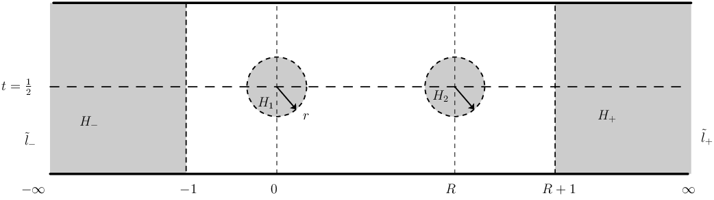
Refer to caption
Figure 5.

where r=ϵ​min⁡(R2,12)r=\epsilon\min(\frac{R}{2},\frac{1}{2}) for some ϵ≪1\epsilon\ll 1. The end e−:(−∞,−1]×[0,1]→ΣR,0e_{-}:(-\infty,-1]\times[0,1]\to\Sigma_{R,0} is the identity map while e+:[1,∞)×[0,1]→ΣR,0e_{+}:[1,\infty)\times[0,1]\to\Sigma_{R,0} shifts by RR to the right. The structure of the ends in the shaded discs labelled by HjH_{j} for j=1,2j=1,2 are given by the following

ej:(−∞,−1]×ℝ/ℤ→ΣR,0:(b,θ)↦s+it=eb+2​π​i​θ+zj,e_{j}:(-\infty,-1]\times{\mathbb{R}}/{\mathbb{Z}}\to\Sigma_{R,0}:(b,\theta)\mapsto s+it=e^{b+2\pi i\theta}+z_{j},

where z1=i2z_{1}=\frac{i}{2} and z2=R+i2z_{2}=R+\frac{i}{2}, and (Hj,𝐉j)(H_{j},\mathbf{J}_{j}) are regular pairs for F​H∗​(M)FH_{*}(M) on the ends eje_{j} for j=1,2j=1,2. The equation (2.8) is obtained when R→0R\to 0 or R→∞R\to\infty, for which we need compact perturbations of the above basic structure. Because the perturbations are restricted in a compact region of the domain, as well as the condition RR excluding bubbling off of discs and spheres, the corresponding operators and resulting moduli spaces (at dimension 00) allow for a cobordism argument, which will establish the equation (2.8).

For R→∞R\to\infty we choose regular pair (H0,𝐉0)(H_{0},\mathbf{J}_{0}) for F​H∗​(M,L)FH_{*}(M,L) and perturb as in figure 6.

Refer to caption
Figure 6.

We write the coordinates explicitly in the region labelled by H0H_{0}:

e0,R:[0,R2]×[0,1]→ΣR,0:(s,t)↦(s+R4,t).e_{0,R}:[0,\frac{R}{2}]\times[0,1]\to\Sigma_{R,0}:(s,t)\mapsto(s+\frac{R}{4},t).

When R→∞R\to\infty, the width of the shaded region labelled by H0H_{0} goes to ∞\infty. This gives the right hand side of (2.8). On the other hand, for R≪1R\ll 1 we choose a regular pair (H3,𝐉3)(H_{3},\mathbf{J}_{3}) for F​H∗​(M)FH_{*}(M) and perturb as in figure 7,

Refer to caption
Figure 7.

where the shaded region labelled by H3H_{3} is an annulus centered at (R2,12)(\frac{R}{2},\frac{1}{2}), for which the outer circle has radius e−1e^{-1} and the inner circle has radius 2​R2R. This region is biholomorphic to the cylinder [ln⁡(2​R),−1]×ℝ/ℤ[\ln(2R),-1]\times{\mathbb{R}}/{\mathbb{Z}} via

e3,R:[ln⁡(2​R),−1]×ℝ/ℤ→ΣR,0:(b,θ)↦s+i​t=eb+2​π​i​θ+12​(R+i),e_{3,R}:[\ln(2R),-1]\times{\mathbb{R}}/{\mathbb{Z}}\to\Sigma_{R,0}:(b,\theta)\mapsto s+it=e^{b+2\pi i\theta}+\frac{1}{2}(R+i),

and we put on the annulus (H3,θ,J3,θ)(H_{3,\theta},J_{3,\theta}) using the cylindrical coordinates given by the map e3,Re_{3,R}. When R→0R\to 0, the length of the above cylinder goes to ∞\infty. This gives the left hand side of (2.8).

The equations we consider are similar to (2.6), where we choose a generic family of pairs (𝐇R,𝐉R)(\mathbf{H}^{R},\mathbf{J}^{R}) where 𝐇R∈C∞​(ΣR,0×M)\mathbf{H}^{R}\in C^{\infty}(\Sigma_{R,0}\times M) and 𝐉R\mathbf{J}^{R} is a family of almost complex structures parametrized by ΣR,0\Sigma_{R,0}, so that its pull-back to the cylindrical parts (the shaded parts in the above diagrams) coincides with the corresponding labellings and restricts to 00 in a neighbourhood of the boundaries of the shaded regions. Then the equation for (u,R)(u,R) have the form:

{∂u∂s+Js,tR​(u)​(∂u∂t−XHs,tR​(u))=0 for ​(s,t)∈ unshaded region,∂u∗∂s+Je∗​(s,t)R​(u∗)​(∂u∗∂t−XHe∗​(s,t)R​(u∗))=0 for ​(s,t)∈ the domain of ​e∗,u|ℝ×{0,1}⊂L\left\{\begin{matrix}\frac{\partial u}{\partial s}+J^{R}_{s,t}(u)\left(\frac{\partial u}{\partial t}-X_{H^{R}_{s,t}}(u)\right)=0&\text{ for }(s,t)\in\text{ unshaded region},\\ \frac{\partial u_{*}}{\partial s}+J^{R}_{e_{*}(s,t)}(u_{*})\left(\frac{\partial u_{*}}{\partial t}-X_{H^{R}_{e_{*}(s,t)}}(u_{*})\right)=0&\text{ for }(s,t)\in\text{ the domain of }e_{*},\\ u|_{{\mathbb{R}}\times\{0,1\}}\subset L\end{matrix}\right. (2.9)

where u∗=u∘e∗u_{*}=u\circ e_{*} and ∗=+,−,1,2,(0,R)when ​R→∞,(3,R)when ​R→0*=+,-,1,2,(0,R)_{\text{when }R\to\infty},(3,R)_{\text{when }R\to 0} respectively. The gluing that relates the limiting configuration to the configuration where R∈(0,∞)R\in(0,\infty) is similar in all respects to the one employed in the literature, e.g. in [3].

We recall here that the pair-of-pants product in F​H∗​(M,ω)FH_{*}(M,\omega) is defined by considering the domain S2∖{0,1,∞}S^{2}\setminus\{0,1,\infty\} (see figure 8).

Refer to caption
Figure 8.

The shaded discs around 00, 11 and ∞\infty are provided with cylindrical coordinates, so that the disc around 00 and 11 are identified with (−∞,−1]×ℝ/ℤ(-\infty,-1]\times{\mathbb{R}}/{\mathbb{Z}} and the one around ∞\infty is identified with [1,∞)×ℝ/ℤ[1,\infty)\times{\mathbb{R}}/{\mathbb{Z}}. To set the order of the multiplication, let γ~j\widetilde{\gamma}_{j} be critical points for the action functional of HjH_{j} for j=1,2j=1,2. Then counting 00-dimensional moduli spaces of maps from the above domain satisfying the perturbed holomorphic equation as described in figure 8 defines the product γ~1∗γ~2\widetilde{\gamma}_{1}*\widetilde{\gamma}_{2}. Comparing this with the description of figure 7, we see that the F​H∗​(M)FH_{*}(M)-action is indeed a right action.

Remark 2.13.

Via the PSS-isomorphism between F​H∗​(M)FH_{*}(M) and Q​H∗​(M)QH_{*}(M), the action described in this section can also be thought of as a right action of Q​H∗​(M)QH_{*}(M) on F​H∗​(M,L)FH_{*}(M,L). In a way similar to the description of the PSS-isomorphism, the action by Q​H∗​(M)QH_{*}(M) can be constructed directly using Morse trajectories as in Biran-Cornea [4].

2.9. Albers’ map

We describe a proof of the following

Proposition 2.14

The action introduced above is compatible with the comparison map 𝒜:F​H∗​(M)→F​H∗​(M,L)\mathscr{A}:FH_{*}(M)\to FH_{*}(M,L) introduced by Albers in [3] via the half-pair-of-pants product, whenever all ingredients are defined. It means

[l~−]∘[γ~0]=[l~−]∗𝒜⁡([γ~0]),[\widetilde{l}_{-}]\circ[\widetilde{\gamma}_{0}]=[\widetilde{l}_{-}]*\mathscr{A}([\widetilde{\gamma}_{0}]),

where [l~−]∈F​H∗​(M,L)[\widetilde{l}_{-}]\in FH_{*}(M,L) and [γ~0]∈F​H∗​(M)[\widetilde{\gamma}_{0}]\in FH_{*}(M).

We consider the domain Σδ=ℝ×[0,1]∖{(0,δ)}\Sigma_{\delta}={\mathbb{R}}\times[0,1]\setminus\{(0,\delta)\}, δ→0\delta\to 0 with the cylindrical structure as in figure 9, where r=ϵ​δr=\epsilon\delta for some ϵ≪1\epsilon\ll 1.

Refer to caption
Figure 9.

We choose a regular pair (H0,𝐉0)(H_{0},\mathbf{J}_{0}) for F​H∗​(M,L)FH_{*}(M,L) and (H1,𝐉1)(H_{1},\mathbf{J}_{1}) for F​H∗​(M)FH_{*}(M). The shaded half-annulus labelled by H0H_{0} is centered at (0,0)(0,0) and outer radius e−2e^{-2} and inner radius is 2​δ2\delta. The cylindrical coordinates on the shaded half-annulus is given by the biholomorphic map

ea,δ:[ln⁡(2​δ)+1,−1]×[0,1]→Σδ:(b,θ)↦s+i​t=eb−1+π​i​θ,e_{a,\delta}:[\ln(2\delta)+1,-1]\times[0,1]\to\Sigma_{\delta}:(b,\theta)\mapsto s+it=e^{b-1+\pi i\theta},

and we put on it (Ha,θ,Ja,θ)(H_{a,\theta},J_{a,\theta}) using ea,δe_{a,\delta}. When δ→0\delta\to 0, the length of the cylinder goes to ∞\infty. We then solve an equation for (u,δ)(u,\delta) of the type (2.9) with the above domain and the cylindrical data. In the limit δ→0\delta\to 0, the domain splits into the domain for the half-pair-of-pants in §2.7 together with the “chimney domain” used to define the map 𝒜\mathscr{A}, see figure 10.

Refer to caption
Figure 10.

Then a gluing argument similar to the one in [3] proves the statement.

The following corollary of proposition 2.14 gives the image of the identity 1∈F​H∗​(M)1\!\!1\in FH_{*}(M) under the comparison map 𝒜\mathscr{A}:

Proposition 2.15

Suppose that identity exists for the half-pair-of-pants product defined in §2.7, then 𝒜⁡(1)=1L\mathscr{A}(1\!\!1)=1\!\!1_{L}.

Proof: According to proposition 2.14, we only have to show that the action of 11\!\!1 on F​H∗​(M,L)FH_{*}(M,L) gives the identity map. We consider the domain in figure 11, for δ≪1\delta\ll 1.

Refer to caption
Figure 11.

When δ>0\delta>0, this again leads to the identity map on the Lagrangian Floer homology F​H∗​(M,L)FH_{*}(M,L). In the limit when δ→0\delta\to 0, the domain splits into two parts, one of which is described in figure 4. The other one is the “capped domain” in the description of PSS map in [13], see figure 12.

Refer to caption
Figure 12.

A similar argument as in §2.7 shows that counting the dimension 00 moduli spaces of caps gives 1∈F​H∗​(M)1\!\!1\in FH_{*}(M), and a gluing argument then shows that the action of 11\!\!1 on F​H∗​(M,L)FH_{*}(M,L) is indeed the identity map. ∎

3. Seidel’s construction for Lagrangian Floer homology

For the discussion in this section, we impose furthermore the following

Assumption 3.1.

F​H∗​(M,L)FH_{*}(M,L) is non-vanishing, in particular, LL is non-displaceable in MM.

By this assumption, any (time-dependent) Hamiltonian function has contractible flow line connecting points on LL.

3.1. Path group and action

Let HamL​(M,ω){\rm Ham}_{L}(M,\omega) be the subgroup of Ham⁡(M,ω){\rm Ham}(M,\omega) that preserves LL, i.e.

ϕ∈HamL​(M,ω)⇔ϕ∈Ham⁡(M,ω)​ and ​ϕ​(L)=L.\phi\in{\rm Ham}_{L}(M,\omega)\iff\phi\in{\rm Ham}(M,\omega)\text{ and }\phi(L)=L.

We consider the following path group in Ham⁡(M,ω){\rm Ham}(M,\omega):

Definition 3.2.

𝒫L​Ham​(M,ω):={g:([0,1],{0},{1})→(Ham⁡(M,ω),i​d,HamL​(M,ω))}{\mathcal{P}}_{L}{\rm Ham}(M,\omega):=\{g:([0,1];\{0\},\{1\})\to({\rm Ham}(M,\omega);id,{\rm Ham}_{L}(M,\omega))\} is a group with pointwise composition:

(g∘h)t=gt​ht.(g\circ h)_{t}=g_{t}h_{t}.

For g∈𝒫L​Ham​(M,ω)g\in{\mathcal{P}}_{L}{\rm Ham}(M,\omega), the action of it on a path l:([0,1];{0,1})→(M,L)l:([0,1];\{0,1\})\to(M,L) is

(g∘l)​(t)=lg​(t):=gt∘l⁡(t).(g\circ l)(t)=l^{g}(t):=g_{t}\circ l(t).

Suppose that gg is generated by K:[0,1]×M→ℝK:[0,1]\times M\to{\mathbb{R}} then we have g∗​αH=αHgg^{*}\alpha_{H}=\alpha_{H^{g}} and g∗(,)𝐉=(,)𝐉gg^{*}(,)_{\mathbf{J}}=(,)_{\mathbf{J}^{g}} where

Hg​(t,x)=H⁡(t,gt​x)−K⁡(t,gt​x)​ and ​Jtg​(x)=d​gt−1∘Jt​(gt​x)∘d​gt.H^{g}(t,x)=H(t,g_{t}x)-K(t,g_{t}x)\text{ and }J_{t}^{g}(x)=dg_{t}^{-1}\circ J_{t}(g_{t}x)\circ dg_{t}.

In particular, we have (Hg)h=Hg​h(H^{g})^{h}=H^{gh} and (𝐉g)h=𝐉g​h(\mathbf{J}^{g})^{h}=\mathbf{J}^{gh}. Let ϕt\phi_{t} denote the Hamiltonian isotopy generated by HtH_{t}, then HtgH^{g}_{t} generates gt−1​ϕtg^{-1}_{t}\phi_{t}. It follows that the connecting Hamiltonian flow lines of HtH_{t} and HtgH_{t}^{g} are in one-to-one correspondence.

As in Lalonde-McDuff-Polterovich [8] where it is shown that Ham⁡(M){\rm Ham}(M) acts trivially on homology (and sends contractible loops in MM to contractible loops), one sees easily that the same argument shows that the action of 𝒫L​Ham​(M,ω){\mathcal{P}}_{L}{\rm Ham}(M,\omega) on the space of paths preserves the component 𝒫L​M{\mathcal{P}}_{L}M.

Most computations in the following are parallel to the corresponding ones in [16].

Proposition 3.3

The action of 𝒫L​Ham​(M,ω){\mathcal{P}}_{L}{\rm Ham}(M,\omega) on 𝒫L​M{\mathcal{P}}_{L}M can be lifted to an action of 𝒫~L​Ham​(M,ω)\widetilde{{\mathcal{P}}}_{L}{\rm Ham}(M,\omega) on the covering 𝒫~L​M\widetilde{{\mathcal{P}}}_{L}M, where

𝒫~LHam(M,ω):={(g,g~)∈𝒫LHam(M,ω)×Homeo(𝒫~LM)|g~ lifts the action of g}\widetilde{{\mathcal{P}}}_{L}{\rm Ham}(M,\omega):=\left\{\left.(g,\widetilde{g})\in{\mathcal{P}}_{L}{\rm Ham}(M,\omega)\times{\rm Homeo}(\widetilde{{\mathcal{P}}}_{L}M)\right|\widetilde{g}\text{ lifts the action of }g\right\}
Proof.

We only need to show that the action can be lifted. Suppose γ:S1→𝒫L​M\gamma:S^{1}\to{\mathcal{P}}_{L}M is a loop that can be lifted to 𝒫~L​M\widetilde{\mathcal{P}}_{L}M, then it is represented by a map B:(S1×[0,1],S1×{0,1})→(M,L)B:\left(S^{1}\times[0,1],S^{1}\times\{0,1\}\right)\to(M,L), such that ω⁡(B)=μL​(B)=0\omega(B)=\mu_{L}(B)=0. The loop γg={g⁡(γs)}s∈S1\gamma^{g}=\{g(\gamma_{s})\}_{s\in S^{1}} is represented by Bg​(s,t)=gt∘B⁡(s,t)B^{g}(s,t)=g_{t}\circ B(s,t). Because d​gt:(B∗​T​M,∂B∗​T​L)→((Bg)∗​T​M,(∂Bg)∗​T​L)dg_{t}:(B^{*}TM,\partial B^{*}TL)\to((B^{g})^{*}TM,(\partial B^{g})^{*}TL) is an isomorphism of symplectic bundles preserving the Lagrangian boundary conditions, it follows that μL​(Bg)=μL​(B)=0\mu_{L}(B^{g})=\mu_{L}(B)=0. We compute (Bg)∗​ω=ω⁡(∂Bg∂s,∂Bg∂t)​d​s∧d​t=B∗​ω+d​θ(B^{g})^{*}\omega=\omega\left(\frac{\partial B^{g}}{\partial s},\frac{\partial B^{g}}{\partial t}\right)ds\wedge dt=B^{*}\omega+d\theta with θ=K⁡(t,Bg​(s,t))​d​t\theta=K(t,B^{g}(s,t))dt. Since θ|∂(S1×[0,1])=0\theta|_{\partial(S^{1}\times[0,1])}=0 we find that ω⁡(Bg)=ω⁡(B)=0\omega(B^{g})=\omega(B)=0. Thus, γg\gamma^{g} again can be lifted to 𝒫~L​M\widetilde{\mathcal{P}}_{L}M, which implies that the action of gg can be lifted. ∎

The groups fit into the exact sequence:

0→ΓL→𝒫~L​Ham​(M,ω)→𝒫L​Ham​(M,ω)→0,0\to\Gamma_{L}\to\widetilde{{\mathcal{P}}}_{L}{\rm Ham}(M,\omega)\to{\mathcal{P}}_{L}{\rm Ham}(M,\omega)\to 0,

and passing to homotopy, we get the exact sequence:

ΓL→π~1​(Ham⁡(M,ω),HamL​(M,ω))→π1​(Ham⁡(M,ω),HamL​(M,ω))→0.\Gamma_{L}\to\widetilde{\pi}_{1}({\rm Ham}(M,\omega),{\rm Ham}_{L}(M,\omega))\to\pi_{1}({\rm Ham}(M,\omega),{\rm Ham}_{L}(M,\omega))\to 0.

Let l~=[l,w]∈𝒫~L​M\widetilde{l}=[l,w]\in\widetilde{\mathcal{P}}_{L}M (not necessarily a critical point of any functional) and Φz:Tw⁡(z)​M→ℂn\Phi_{z}:T_{w(z)}M\to{\mathbb{C}}^{n} be any trivialization satisfying Φr:Tw⁡(r)​L→ℝn\Phi_{r}:T_{w(r)}L\to{\mathbb{R}}^{n} for r∈[−1,1]r\in[-1,1]. Let Φzg~\Phi^{\widetilde{g}}_{z} be a similar trivialization defined for l~g~=[lg,wg~]\widetilde{l}^{\widetilde{g}}=[l^{g},w^{\widetilde{g}}]. Now consider

Gt=Φei​π​tg~∘d​gt∘Φei​π​t−1:ℂn→ℂn.G_{t}=\Phi^{\widetilde{g}}_{e^{i\pi t}}\circ dg_{t}\circ\Phi_{e^{i\pi t}}^{-1}:{\mathbb{C}}^{n}\to{\mathbb{C}}^{n}.

Then {Gt​ℝn}\{G_{t}{\mathbb{R}}^{n}\} is a loop of Lagrangian subspaces in ℂn{\mathbb{C}}^{n}. The following definition then does not depend on either the trivialization or the choice of l~\widetilde{l}.

Definition 3.4.

The Maslov degree of g~\widetilde{g} is μ⁡(g~)=μ⁡(Gt​ℝn)\mu(\widetilde{g})=\mu(G_{t}{\mathbb{R}}^{n}). ∎

Proposition 3.5

Let l~=[l,w]\widetilde{l}=[l,w] be a critical point of aHga_{H^{g}}, then l~g~\widetilde{l}^{\widetilde{g}} is a critical point of aHa_{H}. Furthermore, l~\widetilde{l} is non-degenerate if and only if l~g~\widetilde{l}^{\widetilde{g}} is so. For such critical points, we have μ⁡(g~)=μH​(l~g~)−μHg​(l~)\mu(\widetilde{g})=\mu_{H}(\widetilde{l}^{\widetilde{g}})-\mu_{H^{g}}(\widetilde{l}). It follows that μ:g~↦μ⁡(g~)\mu:\widetilde{g}\mapsto\mu(\widetilde{g}) defines a group homomoprhism μ:π~1​(Ham⁡(M,ω),HamL​(M,ω))→ℤ\mu:\widetilde{\pi}_{1}({\rm Ham}(M,\omega),{\rm Ham}_{L}(M,\omega))\to{\mathbb{Z}}.

Proof.

A direct computation from the definitions establish the first statement of the proposition. Suppose ll is non-degenerate, then d​g1−1∘d​ϕ1​(Tl⁡(0)​L)⋔Tl⁡(1)​L⇔d​ϕ1​(Tl⁡(0)​L)⋔Tlg​(1)​Ldg_{1}^{-1}\circ d\phi_{1}(T_{l(0)}L)\pitchfork T_{l(1)}L\iff d\phi_{1}(T_{l(0)}L)\pitchfork T_{l^{g}(1)}L since d​g1dg_{1} preserves T​LTL, and so the second statement follows.

Let l~g~=[lg,wg]\widetilde{l}^{\widetilde{g}}=[l^{g},w^{g}] and Φz:Twg​(z)​M→ℂn\Phi_{z}:T_{w^{g}(z)}M\to{\mathbb{C}}^{n} be a trivialization that defines μH​(l~g~)\mu_{H}(\widetilde{l}^{\widetilde{g}}), then

μH​(l~g~)=μ⁡(Et​ℝn,ℝn), where ​Et=Φei​π​t∘d​ϕt∘Φ1−1:ℂn→ℂn.\mu_{H}(\widetilde{l}^{\widetilde{g}})=\mu(E_{t}{\mathbb{R}}^{n},{\mathbb{R}}^{n}),\text{ where }E_{t}=\Phi_{e^{i\pi t}}\circ d\phi_{t}\circ\Phi_{1}^{-1}:{\mathbb{C}}^{n}\to{\mathbb{C}}^{n}.

Let Φzg:Tw⁡(z)​M→ℂn\Phi^{g}_{z}:T_{w(z)}M\to{\mathbb{C}}^{n} be the trivialization defining μHg​(l~)\mu_{H^{g}}(\widetilde{l}), then

μHg​(l~)=μ⁡(Etg​ℝn,ℝn), where ​Etg=Φei​π​tg∘d​gt−1∘d​ϕt∘(Φ1g)−1:ℂn→ℂn.\mu_{H^{g}}(\widetilde{l})=\mu(E^{g}_{t}{\mathbb{R}}^{n},{\mathbb{R}}^{n}),\text{ where }E^{g}_{t}=\Phi^{g}_{e^{i\pi t}}\circ dg^{-1}_{t}\circ d\phi_{t}\circ\left(\Phi^{g}_{1}\right)^{-1}:{\mathbb{C}}^{n}\to{\mathbb{C}}^{n}.

Suppose Φ1g=Φ1\Phi^{g}_{1}=\Phi_{1} and let Gt−1=Φei​π​tg∘d​gt−1∘Φei​π​t−1G_{t}^{-1}=\Phi^{g}_{e^{i\pi t}}\circ dg^{-1}_{t}\circ\Phi_{e^{i\pi t}}^{-1}, then Et=Gt∘Etg=Gt​#​EtgE_{t}=G_{t}\circ E^{g}_{t}=G_{t}\#E^{g}_{t} because GtG_{t} is a loop. Thus the property of the Maslov index of Lagrangian paths (see [14] theorem 2.32.3) gives

μ⁡(Et​ℝn,ℝn)=μ⁡(Gt)+μ⁡(Etg​ℝn,ℝn)⇒μ⁡(g~)=μH​(l~g~)−μHg​(l~).\mu(E_{t}{\mathbb{R}}^{n},{\mathbb{R}}^{n})=\mu(G_{t})+\mu(E^{g}_{t}{\mathbb{R}}^{n},{\mathbb{R}}^{n})\Rightarrow\mu(\widetilde{g})=\mu_{H}(\widetilde{l}^{\widetilde{g}})-\mu_{H^{g}}(\widetilde{l}).

∎

In a way entirely parallel to [16], we have

Proposition 3.6

For critical points l~−\widetilde{l}_{-}, l~+\widetilde{l}_{+} of aHga_{H^{g}}, there is a bijection of moduli spaces:

ℳHg,𝐉g​(M,L,l~−,l~+)→ℳH,𝐉​(M,L,l~−g,l~+g)u↦ug\begin{matrix}{\mathcal{M}}_{H^{g},\mathbf{J}^{g}}(M,L;\widetilde{l}_{-},\widetilde{l}_{+})&\to&{\mathcal{M}}_{H,\mathbf{J}}(M,L;\widetilde{l}_{-}^{g},\widetilde{l}_{+}^{g})\\ u&\mapsto&u^{g}\end{matrix}

where

ug​(s,t):=gt∘u⁡(s,t).u^{g}(s,t):=g_{t}\circ u(s,t). (3.1)

Furthermore, (H,𝐉)(H,\mathbf{J}) is regular iff (Hg,𝐉g)(H^{g},\mathbf{J}^{g}) is. The map F​C∗​(g~,H,𝐉)FC_{*}(\widetilde{g};H,\mathbf{J}) defined by ⟨l~⟩↦⟨l~g⟩{\langle}\widetilde{l}{\rangle}\mapsto{\langle}\widetilde{l}^{g}{\rangle} passes to homology:

F​H∗​(g~):F​H∗​(Hg,𝐉g)→F​H∗+μ⁡(g~)​(H,𝐉)FH_{*}(\widetilde{g}):FH_{*}(H^{g},\mathbf{J}^{g})\to FH_{*+\mu(\widetilde{g})}(H,\mathbf{J})

and defines an automorphism of F​H∗​(M,L)FH_{*}(M,L) of degree μ⁡(g~)\mu(\widetilde{g}). Furthermore the following hold:

  1. (1)

    for (g,g~)=(i​d,i​d)(g,\widetilde{g})=(id,id), F​H∗​(g~)=i​dFH_{*}(\widetilde{g})=id,

  2. (2)

    for (g,g~)=(i​d,β)(g,\widetilde{g})=(id,\beta) with β∈ΓL\beta\in\Gamma_{L}, we have F​H∗​(g~)=β⋅i​dFH_{*}(\widetilde{g})=\beta\cdot id,

  3. (3)

    F​H∗​(g~)FH_{*}(\widetilde{g}) is a ΛL\Lambda_{L}-module automorphism of degree μ⁡(g~)\mu(\widetilde{g}),

  4. (4)

    F​H∗​(g~∘g~′)=F​H∗​(g~)∘F​H∗​(g~′)FH_{*}(\widetilde{g}\circ\widetilde{g}^{\prime})=FH_{*}(\widetilde{g})\circ FH_{*}(\widetilde{g}^{\prime}).

∎

3.2. Homotopy invariance

We consider a smooth path {gr}r∈[0,1]\{g_{r}\}_{r\in[0,1]} starting from the identity in 𝒫L​Ham​(M,ω){\mathcal{P}}_{L}{\rm Ham}(M,\omega) and a lift {(gr,g~r)}\{(g_{r},\widetilde{g}_{r})\} of it to 𝒫~L​Ham​(M,ω)\widetilde{\mathcal{P}}_{L}{\rm Ham}(M,\omega). Then proposition 3.5 implies that μ⁡(g~r)=0\mu(\widetilde{g}_{r})=0 for all r∈[0,1]r\in[0,1]. The path {gr}\{g_{r}\} corresponds to a smooth family {gr,t}(r,t)∈[0,1]2\{g_{r,t}\}_{(r,t)\in[0,1]^{2}} of Hamiltonian diffeomorphisms in Ham⁡(M,ω){\rm Ham}(M,\omega) so that

g0,t=gr,0=i​d​ and ​gr,1∈HamL​(M,ω)​ for all ​r∈[0,1].g_{0,t}=g_{r,0}=id\text{ and }g_{r,1}\in{\rm Ham}_{L}(M,\omega)\text{ for all }r\in[0,1].

Choose a smooth family of Hamiltonians Kr:[0,1]×M→ℝK_{r}:[0,1]\times M\to{\mathbb{R}} for r∈[0,1]r\in[0,1] so that KrK_{r} generates grg_{r} and K0=0K_{0}=0. Let

Hgr​(t,x)=H⁡(t,gr,t​(x))−Kr​(t,gt,r​(x))​ and ​Jtgr=d​gr,t−1∘Jt​(gr,t​(x))∘d​gr,tH^{g_{r}}(t,x)=H(t,g_{r,t}(x))-K_{r}(t,g_{t,r}(x))\text{ and }J_{t}^{g_{r}}=dg_{r,t}^{-1}\circ J_{t}(g_{r,t}(x))\circ dg_{r,t}

Let (H0,𝐉0)={(Ht,Jt)}t∈[0,1](H_{0},\mathbf{J}_{0})=\{(H_{t},J_{t})\}_{t\in[0,1]} and (H1,𝐉1)={(Htg1,Jtg1)}t∈[0,1](H_{1},\mathbf{J}_{1})=\{(H^{g_{1}}_{t},J^{g_{1}}_{t})\}_{t\in[0,1]}, then the construction in the last subsection gives

F​H∗​(g~1):F​H∗​(H1,𝐉1)→F​H∗​(H0,𝐉0).FH_{*}(\widetilde{g}_{1}):FH_{*}(H_{1},\mathbf{J}_{1})\to FH_{*}(H_{0},\mathbf{J}_{0}).

Let (H¯,𝐉¯)={(Hs,t,Js,t)}(s,t)∈ℝ×[0,1](\bar{H},\bar{\mathbf{J}})=\{(H_{s,t},J_{s,t})\}_{(s,t)\in{\mathbb{R}}\times[0,1]} be a regular homotopy connecting (H0,𝐉0)(H_{0},\mathbf{J}_{0}) and (H1,𝐉1)(H_{1},\mathbf{J}_{1}):

(H¯s,𝐉¯s)={(H1,𝐉1)s⩽−1(H0,𝐉0)s⩾1.(\bar{H}_{s},\bar{\mathbf{J}}_{s})=\left\{\begin{matrix}(H_{1},\mathbf{J}_{1})&s{\leqslant}-1\\ (H_{0},\mathbf{J}_{0})&s{\geqslant}1\end{matrix}\right..

We consider the moduli spaces of the solutions of the following equation for maps u:ℝ×[0,1]→Mu:{\mathbb{R}}\times[0,1]\to M with ∂u:ℝ×{0,1}→L\partial u:{\mathbb{R}}\times\{0,1\}\to L:

∂u∂s+Js,t​(u)​(∂u∂t−XHs,t​(u))=0.\frac{\partial u}{\partial s}+J_{s,t}(u)\left(\frac{\partial u}{\partial t}-X_{H_{s,t}}(u)\right)=0.

Here (H¯,𝐉¯)(\bar{H},\bar{\mathbf{J}}) being regular means that all solutions uu are regular, i.e. their linearizations are surjective. The moduli space ℳH¯,𝐉¯​(M,L,l~−,l~+){\mathcal{M}}_{\bar{H},\bar{\mathbf{J}}}(M,L;\widetilde{l}_{-},\widetilde{l}_{+}) denotes the space of solutions uu that converge to Hamiltonian paths when s→±∞s\to\pm\infty:

lims→−∞=l~−g1−1 and lims→+∞=l~+,\lim_{s\to-\infty}=\widetilde{l}_{-}^{g_{1}^{-1}}\text{ and }\lim_{s\to+\infty}=\widetilde{l}_{+},

where l~±\widetilde{l}_{\pm} are critical points of aHa_{H}. The dimension of the moduli space is given by

μH​(l~−)−μH​(l~+),\mu_{H}(\widetilde{l}_{-})-\mu_{H}(\widetilde{l}_{+}),

since there is no ℝ{\mathbb{R}}-action anymore. Then the continuation map on the chain level

ΦH¯,𝐉¯:F​C∗​(H1)→F​C∗​(H0)\Phi_{\bar{H},\bar{\mathbf{J}}}:FC_{*}(H_{1})\to FC_{*}(H_{0})

is defined by counting dimension 00 moduli spaces:

ΦH¯,𝐉¯​(l~−g1−1)=∑l~+#​ℳH¯,𝐉¯​(M,L,l~−,l~+)​l~+.\Phi_{\bar{H},\bar{\mathbf{J}}}(\widetilde{l}_{-}^{g_{1}^{-1}})=\sum_{\widetilde{l}_{+}}\#{\mathcal{M}}_{\bar{H},\bar{\mathbf{J}}}(M,L;\widetilde{l}_{-},\widetilde{l}_{+})\widetilde{l}_{+}.

That ΦH¯,𝐉¯\Phi_{\bar{H},\bar{\mathbf{J}}} is a chain map is shown by considering the dimension 11 moduli spaces. Thus we have the continuation map for Floer homology, which is also denoted ΦH¯,𝐉¯\Phi_{\bar{H},\bar{\mathbf{J}}}. The homotopy invariance of F​H∗​(g~)FH_{*}(\widetilde{g}) is equivalent to the following:

Proposition 3.7

With the above setup, we have F​H∗​(g~1)=ΦH¯,𝐉¯FH_{*}(\widetilde{g}_{1})=\Phi_{\bar{H},\bar{\mathbf{J}}}.

As in [16], we consider the deformation of homotopies, from the trivial homotopy to (H¯,𝐉¯)(\bar{H},\bar{\mathbf{J}}) by the curve {(gr,g~r)}\{(g_{r},\widetilde{g}_{r})\}, which is a family (H~,J~)={(Hr,s,t,Jr,s,t)}(r,s,t)∈[0,1]×ℝ×[0,1](\widetilde{H},\widetilde{J})=\{(H_{r,s,t},J_{r,s,t})\}_{(r,s,t)\in[0,1]\times{\mathbb{R}}\times[0,1]} where

Hr,s,t​(x)=Htgr​(x),\displaystyle H_{r,s,t}(x)=H^{g_{r}}_{t}(x), Jr,s,t​(x)=Jtgr​(x)\displaystyle J_{r,s,t}(x)=J^{g_{r}}_{t}(x) for ​s⩽−1\displaystyle\text{ for }s{\leqslant}-1
Hr,s,t​(x)=Ht​(x),\displaystyle H_{r,s,t}(x)=H_{t}(x), Jr,s,t​(x)=Jt​(x)\displaystyle J_{r,s,t}(x)=J_{t}(x) for ​s⩾1\displaystyle\text{ for }s{\geqslant}1
H0,s,t​(x)=Ht​(x),\displaystyle H_{0,s,t}(x)=H_{t}(x), J0,s,t​(x)=Jt​(x)\displaystyle J_{0,s,t}(x)=J_{t}(x) and
H1,s,t​(x)=Hs,t​(x)\displaystyle H_{1,s,t}(x)=H_{s,t}(x) J1,s,t​(x)=Js,t​(x)\displaystyle J_{1,s,t}(x)=J_{s,t}(x)

The equation that we are now concerned with is the following:

∂u∂s+Jr,s,t​(u)​(∂u∂t−XHr,s,t​(u))=0,\frac{\partial u}{\partial s}+J_{r,s,t}(u)\left(\frac{\partial u}{\partial t}-X_{H_{r,s,t}}(u)\right)=0, (3.2)

for the pair (r,u)(r,u), where r∈[0,1]r\in[0,1] and u:ℝ×[0,1]→Mu:{\mathbb{R}}\times[0,1]\to M with ∂u:ℝ×{0,1}→L\partial u:{\mathbb{R}}\times\{0,1\}\to L. Let ℳH~,𝐉~​(M,L,l~−,l~+){\mathcal{M}}_{\widetilde{H},\widetilde{\mathbf{J}}}(M,L;\widetilde{l}_{-},\widetilde{l}_{+}) denote the moduli space of solutions (r,u)(r,u) so that uu solves the equation at the parameter rr and converges to Hamiltonian paths as s→±∞s\to\pm\infty, i.e.:

lims→−∞=l~−gr−1 and lims→+∞=l~+,\lim_{s\to-\infty}=\widetilde{l}_{-}^{g_{r}^{-1}}\text{ and }\lim_{s\to+\infty}=\widetilde{l}_{+},

where l~±\widetilde{l}_{\pm} are critical points of aHa_{H}. Then the expected dimension of this moduli space is

μH​(l~−)−μH​(l~+)+1,\mu_{H}(\widetilde{l}_{-})-\mu_{H}(\widetilde{l}_{+})+1,

because of the extra parameter rr. The deformation of homotopies is said to be regular if the linearized operator for (3.2) is surjective for all (r,u)(r,u) and no bubbling off of either spheres or discs occur for the moduli spaces with dimension ⩽1{\leqslant}1. We note that here the monotonicity guarantees the existence of regular deformation of homotopies. ∎

3.3. Module property and Seidel element

Proposition 3.8

The map F​H∗​(g~)FH_{*}(\tilde{g}) is a module map with respect to the half pair of pants product on F​H∗​(M,L)FH_{*}(M,L), i.e. for [l~−],[l~0]∈F​H∗​(M,L)[\tilde{l}_{-}],[\tilde{l}_{0}]\in FH_{*}(M,L), we have

F​H∗​(g~)​([l~−]∗[l~0])=F​H∗​(g~)​([l~−])∗[l~0]FH_{*}(\tilde{g})([\tilde{l}_{-}]*[\tilde{l}_{0}])=FH_{*}(\tilde{g})([\tilde{l}_{-}])*[\tilde{l}_{0}]

Proof: Because of the homotopy invariance, we may reparametrize gg so that gt=i​dg_{t}=id for t∈[0,12]t\in[0,\frac{1}{2}]. Consider the half pair of pants product defined by the punctured strip as in Figure 1, §2.7. Let (𝐇,𝐉)(\mathbf{H},\mathbf{J}) be a regular pair which pulls back to the ends e±e_{\pm} and e0e_{0} respectively as (H±,J±)(H_{\pm},J_{\pm}) and (H0,J0)(H_{0},J_{0}). Then the pair (𝐇g,𝐉g)(\mathbf{H}^{g},\mathbf{J}^{g}) defined by

𝐇g​(s,t,x):=𝐇⁡(s,t,gt​x)−K⁡(s,t,gt​x)​ and ​𝐉g​(s,t,x):=d​gt−1∘𝐉s,t​(x)∘d​gt\mathbf{H}^{g}(s,t,x):=\mathbf{H}(s,t,g_{t}x)-K(s,t,g_{t}x)\text{ and }\mathbf{J}^{g}(s,t,x):=dg_{t}^{-1}\circ\mathbf{J}_{s,t}(x)\circ dg_{t}

pulls back to the ends e±e_{\pm} and e0e_{0} respectively as (H±g,J±g)(H^{g}_{\pm},J^{g}_{\pm}) and (H0,J0)(H_{0},J_{0}). Let l~±g\tilde{l}^{g}_{\pm} and l~±\tilde{l}_{\pm} be critical points of the action functionals aH±a_{H_{\pm}} and aH±ga_{H^{g}_{\pm}} respectively and l~0\tilde{l}_{0} a critical point of aH0a_{H_{0}}. We then have the isomorphism of moduli spaces as in Proposition 3.6

ℳ𝐇g,𝐉g​(M,L,l~−,l~0,l~+)≅ℳ𝐇,𝐉​(M,L,l~−g,l~0,l~+g):u↦ug,\mathcal{M}_{\mathbf{H}^{g},\mathbf{J}^{g}}(M,L;\tilde{l}_{-},\tilde{l}_{0},\tilde{l}_{+})\cong\mathcal{M}_{\mathbf{H},\mathbf{J}}(M,L;\tilde{l}_{-}^{g},\tilde{l}_{0},\tilde{l}_{+}^{g}):u\mapsto u^{g},

where ug​(s,t):=gt∘u⁡(s,t)u^{g}(s,t):=g_{t}\circ u(s,t). The statement then follows. ∎

From the properties in proposition 3.6 and the homotopy invariance, we may define similarly the Seidel element for the Lagrangian Floer homology. Here we have to assume more:

Definition 3.9.

Suppose that F​H∗​(M,L)FH_{*}(M,L) is non-zero and has an identity element with respect to the half-pair-of-pants product defined above, which is denoted 1L1\!\!1_{L}. Then

F​Ψg~,L:=F​H∗​(g~)​(1L)∈F​H∗​(M,L)F\Psi_{\widetilde{g},L}:=FH_{*}(\widetilde{g})(1\!\!1_{L})\in FH_{*}(M,L)

is the Seidel element for the class [g~]∈π~1​(Ham⁡(M,ω),H​a​mL​(M,ω))[\widetilde{g}]\in\widetilde{\pi}_{1}({\rm Ham}(M,\omega),Ham_{L}(M,\omega)).

It follows that in this case, for [l~]∈F​H∗​(M,L)[\widetilde{l}]\in FH_{*}(M,L) we have

F​H∗​(g~)​([l~])=F​Ψg~,L∗[l~].FH_{*}(\widetilde{g})([\widetilde{l}])=F\Psi_{\widetilde{g},L}*[\widetilde{l}].

The assumption above is satisfied in many cases, for example the diagonal in M×MM\times M.

3.4. Hamiltonian fibrations over a disc

The unit disc D2D^{2} in ℂ{\mathbb{C}} can be parametrized by the upper half plane ℍ¯\bar{\mathbb{H}} compactified by ℝ{\mathbb{R}} and a point at ∞\infty.

Notation 3.1.

The following notations are only used in this section. They are NOT compatible with the notations for the same objects used elsewhere in this paper. In the parametrization by ℍ{\mathbb{H}}, let

D±2={z∈ℍ¯|±(|z|−1)⩾0}.D^{2}_{\pm}=\{z\in\bar{\mathbb{H}}|\pm(|z|-1){\geqslant}0\}.

The two half discs can be identified by the map:

D+2→D−2:z↦z¯−1​ or ​r​ei​θ↦r−1​ei​θ.D^{2}_{+}\to D^{2}_{-}:z\mapsto{\bar{z}}^{-1}\text{ or }re^{i\theta}\mapsto r^{-1}e^{i\theta}.

We consider the fibration over D2D^{2} defined from an element g∈𝒫L​Ham​(M,ω)g\in{\mathcal{P}}_{L}{\rm Ham}(M,\omega):

Pg=M×D+2⊔M×D−2/∼:(x,ei​π​t)∼(gt(x),ei​π​t) for t∈[0,1].P_{g}=M\times D^{2}_{+}\sqcup M\times{D^{2}_{-}}/\sim:(x,e^{i\pi t})\sim(g_{t}(x),e^{i\pi t})\text{ for }t\in[0,1].

Let π:Pg→D2\pi:P_{g}\to D^{2} denote the projection. We note that along the S1S^{1}-boundary, we have the restricted bundle NN that is obtained as the union of the copies of LL in each fiber; it is a Lagrangian submanifold of PP. Note that N≃L×S1N\simeq L\times S^{1} over S1S^{1} if the restriction of g1g_{1} to LL is diffeotopic to the identity. A choice of the lifting g~∈𝒫~L​Ham​(M,ω)\widetilde{g}\in\widetilde{\mathcal{P}}_{L}{\rm Ham}(M,\omega) amounts again to the choice of a section class σg~\sigma_{\widetilde{g}} in π2​(Pg,N)\pi_{2}(P_{g},N) as follows. For x∈Lx\in L, consider l~=[x,x]∈𝒫~L\widetilde{l}=[x,x]\in\widetilde{\mathcal{P}}_{L} and let l~g~=[gt​(x),w]\widetilde{l}^{\widetilde{g}}=[g_{t}(x),w] with

w:D+2→M:w⁡(ei​π​t)=gt​(x).w:D^{2}_{+}\to M:w(e^{i\pi t})=g_{t}(x).

Via the identification of D±2D^{2}_{\pm}, we write

w−:D−2→M:w−​(z)=w⁡(z¯−1),w_{-}:D^{2}_{-}\to M:w_{-}(z)=w({\bar{z}}^{-1}),

in particular, w−​(ei​π​t)=gt​(x)w_{-}(e^{i\pi t})=g_{t}(x) as well. Now the following section in PgP_{g} represents σg~\sigma_{\widetilde{g}}:

{x}⊔{w−}/∼:(x,ei​π​t)∼(gt(x),ei​π​t) for t∈[0,1],\{x\}\sqcup\{w_{-}\}/\sim:(x,e^{i\pi t})\sim(g_{t}(x),e^{i\pi t})\text{ for }t\in[0,1],

where, for example, {w−}\{w_{-}\} denotes the graph of the map w−w_{-}.

Definition 3.10.

Let the smooth map u:D2→Pgu:D^{2}\to P_{g} represent B∈π2​(Pg,N)B\in\pi_{2}(P_{g},N). The vertical Maslov index of BB, denoted μv​(B)\mu^{v}(B) is the Maslov index of the bundle pair (u∗​Tv​Pg,(∂u)∗​Tv​N)(u^{*}T^{v}P_{g},(\partial u)^{*}T^{v}N), where Tv=ker⁡d​πT^{v}=\ker d\pi denotes the respective vertical tangent bundles.

It’s not hard to show that the above is well defined and not dependent on the choice of a smooth map uu. We then have the following

Proposition 3.11

μ⁡(g~)=μv​([σg~])\mu(\widetilde{g})=\mu^{v}([\sigma_{\widetilde{g}}]).

Proof: The trivial Lagrangian path Txv​N=Tx​LT^{v}_{x}N=T_{x}L over D+2D^{2}_{+} is isotopied to Gt​(x)​ℝnG_{t}(x){\mathbb{R}}^{n} over D−2D^{2}_{-}, via any trivialization chosen for u∗​Tv​Pgu^{*}T^{v}P_{g}. The proposition follows from the definitions. ∎

Remark 3.12.

Since we will not need it in this article, we leave to the reader to check that the definition of the action of the paths in 𝒫L​Ham​(M,ω){\mathcal{P}}_{L}{\rm Ham}(M,\omega) on the relative Floer homology can be interpreted in a geometric way on this bundle over the 2-disc, roughly as the absolute Seidel morphism was interpreted in Lalonde-McDuff-Polterovich [8] as a map from the quantum homology of the fiber at the north pole to the quantum homology of the fiber at the south pole in a fibration over the 2-sphere.

For this purpose, one considers the fibers (M±1,L±1)=π−1​(±1)(M_{\pm 1},L_{\pm 1})=\pi^{-1}(\pm 1). The natural map from F​H∗​(M1,L1)FH_{*}(M_{1},L_{1}) to F​H∗​(M−1,L−1)FH_{*}(M_{-1},L_{-1}) can be defined by the pearl complex (i.e. linear clusters). Namely, one flows inside M1M_{1} from a critical point of the Morse function on L1L_{1} in a linear cluster until that cluster reaches a pseudo-holomorphic section σ\sigma of PP with boundary on NN; then flows along a linear cluster in the fiber M−1M_{-1}, starting from the point σ∩M−1∈L−1\sigma\cap M_{-1}\in L_{-1}, until it reaches some critical point of the Morse function on L−1⊂M−1L_{-1}\subset M_{-1}.

3.5. Compatibility among the actions

We start by noting the obvious inclusion:

Ω0​Ham​(M,ω)⊂𝒫L​Ham​(M,ω),\Omega_{0}{\rm Ham}(M,\omega)\subset{\mathcal{P}}_{L}{\rm Ham}(M,\omega),

where Ω0​Ham​(M,ω)\Omega_{0}{\rm Ham}(M,\omega) denotes the group of smooth loops in Ham⁡(M,ω){\rm Ham}(M,\omega) based at the identity. Recall that in [16], the covering Ω~0​Ham​(M,ω)\widetilde{\Omega}_{0}{\rm Ham}(M,\omega) is defined as following (cf. proposition 3.3):

Ω~0Ham(M,ω):={(g,g~)∈Ω0Ham(M,ω)×Homeo(Ω~M)|g~ lifts the action of g}.\widetilde{\Omega}_{0}{\rm Ham}(M,\omega):=\{\left.(g,\widetilde{g})\in\Omega_{0}{\rm Ham}(M,\omega)\times{\rm Homeo}(\widetilde{\Omega}M)\right|\widetilde{g}\text{ lifts the action of }g\}.
Lemma 3.13

We have the inclusion of groups

Ω~0​Ham​(M,ω)⊂𝒫~L​Ham​(M,ω),\widetilde{\Omega}_{0}{\rm Ham}(M,\omega)\subset\widetilde{\mathcal{P}}_{L}{\rm Ham}(M,\omega),

extending the inclusion Γω→𝑖ΓL\Gamma_{\omega}\xrightarrow{i}\Gamma_{L} in §2.1.

Proof: We show that

Ω~0​Ham​(M,ω)⊂𝒫~L0​Ham​(M,ω),\widetilde{\Omega}_{0}{\rm Ham}(M,\omega)\subset\widetilde{\mathcal{P}}^{0}_{L}{\rm Ham}(M,\omega),

where

𝒫~L0Ham(M,ω):={(g,g~)∈𝒫~LHam(M,ω)|g1|L=id∈Diff(L)}.\widetilde{\mathcal{P}}^{0}_{L}{\rm Ham}(M,\omega):=\left\{\left.(g,\widetilde{g})\in\widetilde{\mathcal{P}}_{L}{\rm Ham}(M,\omega)\right|g_{1}|_{L}={\rm id}\in{\rm Diff}(L)\right\}.

Let

ΩL​M=Ω​M∩𝒫L​M\Omega_{L}M=\Omega M\cap{\mathcal{P}}_{L}M

be the space of loops in MM starting at points in LL. Then an element of Ω0​Ham​(M,ω)\Omega_{0}{\rm Ham}(M,\omega) or 𝒫L​Ham​(M,ω){\mathcal{P}}_{L}{\rm Ham}(M,\omega) is determined by how it acts on ΩL​M\Omega_{L}M. This fact gives a definition of the inclusion Ω0​Ham​(M,ω)↪𝒫L​Ham​(M,ω)\Omega_{0}{\rm Ham}(M,\omega)\hookrightarrow{\mathcal{P}}_{L}{\rm Ham}(M,\omega).

Let π:Ω~​M→Ω​M\pi:\widetilde{\Omega}M\to\Omega M and πL:𝒫~L​M→𝒫L​M\pi_{L}:\widetilde{\mathcal{P}}_{L}M\to{\mathcal{P}}_{L}M be the covering projections. Consider

Ω~L​M:=π−1​(ΩL​M)​ and ​𝒫~L0​M:=πL−1​(ΩL​M).\widetilde{\Omega}_{L}M:=\pi^{-1}(\Omega_{L}M)\text{ and }\widetilde{\mathcal{P}}_{L}^{0}M:=\pi_{L}^{-1}(\Omega_{L}M).

Then by definition, we have

Ω~LM={(l,wΩ)|l∈ΩLM and wΩ:(D2,S1)→(M,l)}/∼Ω\widetilde{\Omega}_{L}M=\{(l,w_{\Omega})|l\in\Omega_{L}M\text{ and }w_{\Omega}:(D^{2},S^{1})\to(M,l)\}/\sim_{\Omega}
𝒫~L0M={(l,w𝒫)|l∈ΩLM and w𝒫:(D+2;∂+,∂0)→(M;l,L)}/∼𝒫\widetilde{\mathcal{P}}_{L}^{0}M=\{(l,w_{\mathcal{P}})|l\in\Omega_{L}M\text{ and }w_{\mathcal{P}}:(D^{2}_{+};\partial_{+},\partial_{0})\to(M;l,L)\}/\sim_{\mathcal{P}}

where

wΩ∼ΩwΩ′⇔Iω(vΩ)=Ic(vΩ)=0 for vΩ=wΩ#(−wΩ′)w_{\Omega}\sim_{\Omega}w^{\prime}_{\Omega}\iff I_{\omega}(v_{\Omega})=I_{c}(v_{\Omega})=0\text{ for }v_{\Omega}=w_{\Omega}\#(-w^{\prime}_{\Omega})
w𝒫∼𝒫w𝒫′⇔Iω(v𝒫)=Iμ(v𝒫)=0 for v𝒫=w𝒫#(−w𝒫′)w_{\mathcal{P}}\sim_{\mathcal{P}}w^{\prime}_{\mathcal{P}}\iff I_{\omega}(v_{\mathcal{P}})=I_{\mu}(v_{\mathcal{P}})=0\text{ for }v_{\mathcal{P}}=w_{\mathcal{P}}\#(-w^{\prime}_{\mathcal{P}})

Let’s choose and fix a smooth map

ι:(D+2;∂+,∂0)→(D2;S1,{1})\iota:(D^{2}_{+};\partial_{+},\partial_{0})\to(D^{2};S^{1},\{1\})

which contracts ∂0\partial_{0} to {1}\{1\} and is an isomorphism otherwise. We have for wΩw_{\Omega}

w~Ω:=wΩ∘ι:(D+2;∂+,∂0)→(M;l,L),\widetilde{w}_{\Omega}:=w_{\Omega}\circ\iota:(D^{2}_{+};\partial_{+},\partial_{0})\to(M;l,L),

as well as

wΩ∼Ωw′Ω⇔w~Ω∼𝒫w~′Ω.w_{\Omega}\sim_{\Omega}w^{\prime}_{\Omega}\iff\widetilde{w}_{\Omega}\sim_{\mathcal{P}}\widetilde{w}^{\prime}_{\Omega}.

The “⇒\Rightarrow” above is obvious. The “⇐\Leftarrow” is because that Iμ=2​IcI_{\mu}=2I_{c} on the maps of the form w~Ω​#​(−w~Ω′)\widetilde{w}_{\Omega}\#(-\widetilde{w}^{\prime}_{\Omega}). In particular, ι\iota induces an inclusion ι∗:Ω~L​M→𝒫~L0​M\iota_{*}:\widetilde{\Omega}_{L}M\to\widetilde{\mathcal{P}}_{L}^{0}M.

On the other hand, for w𝒫w_{\mathcal{P}} as above, we define ∂0w𝒫\partial_{0}w_{\mathcal{P}} by

w𝒫|∂0:([−1,1],{±1})→([−1,1]/{±1},{[1]})→∂0w𝒫(L,l⁡(0)=l⁡(1)).w_{\mathcal{P}}|_{\partial_{0}}:([-1,1],\{\pm 1\})\to([-1,1]/\{\pm 1\},\{[1]\})\xrightarrow{\partial_{0}w_{\mathcal{P}}}(L,l(0)=l(1)).

We then see that ∂0:w𝒫↦∂0w𝒫\partial_{0}:w_{\mathcal{P}}\mapsto\partial_{0}w_{\mathcal{P}} defines a map

∂0∗:𝒫~L0​M→π1​(L)/K\partial_{0}^{*}:\widetilde{\mathcal{P}}_{L}^{0}M\to\pi_{1}(L)/K

where KK is the image of ker⁡Iω∩ker⁡Iμ\ker I_{\omega}\cap\ker I_{\mu} under the map π2​(M,L)→π1​(L)\pi_{2}(M,L)\to\pi_{1}(L), and there is the exact sequence

0→Ω~L​M→ι∗𝒫~L0​M→∂0∗π1​(L)/K.0\to\widetilde{\Omega}_{L}M\xrightarrow{\iota_{*}}\widetilde{\mathcal{P}}_{L}^{0}M\xrightarrow{\partial_{0}^{*}}\pi_{1}(L)/K.

It follows that 𝒫~L0​M\widetilde{\mathcal{P}}_{L}^{0}M is a disjoint union of copies of Ω~L​M\widetilde{\Omega}_{L}M.

Now an element in Ω~0​Ham​(M,ω)\widetilde{\Omega}_{0}{\rm Ham}(M,\omega) is determined by its action on Ω~L​M\widetilde{\Omega}_{L}M and one in 𝒫~L0​Ham​(M,ω)\widetilde{\mathcal{P}}^{0}_{L}{\rm Ham}(M,\omega) by its action on 𝒫~L0​M\widetilde{\mathcal{P}}_{L}^{0}M. It follows that Ω~0​Ham​(M,ω)\widetilde{\Omega}_{0}{\rm Ham}(M,\omega) is the subgroup of 𝒫~L0​Ham​(M,ω)\widetilde{\mathcal{P}}^{0}_{L}{\rm Ham}(M,\omega) preserving each copy of Ω~L​M\widetilde{\Omega}_{L}M in 𝒫~L0​M\widetilde{\mathcal{P}}_{L}^{0}M. The rest of the statement is obvious. ∎

Remark 3.14.

From the lemma, we obtain the exact sequence described in (1.1):

π~1​Ham​(M,ω)→π~1​(Ham⁡(M,ω),HamL​(M,ω))→π~0​HamL​(M,ω)→0,\widetilde{\pi}_{1}{\rm Ham}(M,\omega)\to\widetilde{\pi}_{1}({\rm Ham}(M,\omega),{\rm Ham}_{L}(M,\omega))\to\widetilde{\pi}_{0}{\rm Ham}_{L}(M,\omega)\to 0,

where the third term is the quotient. From the extension sequences of the first two groups and from the triviality of π0​Ham​(M,ω)\pi_{0}{\rm Ham}(M,\omega), we have the following extension sequence:

0→Γ′→π~0​HamL​(M,ω)→π0​HamL​(M,ω)→0,0\to\Gamma^{\prime}\to\widetilde{\pi}_{0}{\rm Ham}_{L}(M,\omega)\to\pi_{0}{\rm Ham}_{L}(M,\omega)\to 0,

where Γ′\Gamma^{\prime} is a quotient of ΓL\Gamma_{L}.

Theorem 3.15

Let [γ~]∈F​H∗​(M,ω)[\widetilde{\gamma}]\in FH_{*}(M,\omega) and g~∈Ω~0​Ham​(M,ω)⊂𝒫~L​Ham​(M,ω)\widetilde{g}\in\widetilde{\Omega}_{0}{\rm Ham}(M,\omega)\subset\widetilde{\mathcal{P}}_{L}{\rm Ham}(M,\omega). Then we have 22 2 The same holds for Seidel elements in quantum homology, for which one apply the construction in [10] for the Hamiltonian Seidel elements, while the relative version is obtained from a similar construction in the fibration over a disc. Correspondingly, one needs to consider H2S​(M,ℝ)H_{2}^{S}(M;\mathbb{R}) and H2S​(M,L,ℝ)H_{2}^{S}(M,L;\mathbb{R}) instead of H2S​(M)H_{2}^{S}(M) and H2S​(M,L)H_{2}^{S}(M,L) when defining the Novikov rings.

𝒜⁡(F​H∗​(g~)​([γ~]))=F​H∗​(g~)​𝒜​([γ~]).\mathscr{A}(FH_{*}(\widetilde{g})([\widetilde{\gamma}]))=FH_{*}(\widetilde{g})\mathscr{A}([\widetilde{\gamma}]).

Proof: Recall that the description of the “chimney domain” in [1] as ℝ×[0,1]/∼{\mathbb{R}}\times[0,1]/\sim where (s,0)∼(s,1)(s,0)\sim(s,1) when s⩽0s{\leqslant}0, and the conformal structure at (0,0)(0,0) is given by z\sqrt{z}. The domain is depicted in figure 13, where the shaded left half of the strip has its two boundaries glued together forming a half infinite cylinder. Let (H,𝐉)(H,\mathbf{J}) be a regular pair for both F​H∗​(M)FH_{*}(M) and F​H∗​(M,L)FH_{*}(M,L) so that (Hg,𝐉g)(H^{g},\mathbf{J}^{g}) is also regular for both of the theories.

Refer to caption
Figure 13.

We then consider an equation similar to (2.1):

{∂u∂s+Jtg​(u)​(∂u∂t−XHtg​(u))=0 for all ​(s,t)∈ℝ×[0,1],u⁡(s,0)=u⁡(s,1) for ​s⩽0u|[0,∞)×{0,1}⊂L\left\{\begin{matrix}\frac{\partial u}{\partial s}+J^{g}_{t}(u)\left(\frac{\partial u}{\partial t}-X_{H^{g}_{t}}(u)\right)=0&\text{ for all }(s,t)\in{\mathbb{R}}\times[0,1],\\ u(s,0)=u(s,1)&\text{ for }s\leqslant 0\\ u|_{[0,\infty)\times\{0,1\}}\subset L\end{matrix}\right. (3.3)

Then 𝒜⁡(γ~)\mathscr{A}(\tilde{\gamma}) is defined by counting 00-dimensional moduli spaces of solutions to (3.3).

We note that F​H∗​(g~)​([γ~])FH_{*}(\tilde{g})([\tilde{\gamma}]) is represented by γ~g\tilde{\gamma}^{g} while F​H∗​(g~)​([l~])FH_{*}(\tilde{g})([\tilde{l}]) by l~g\tilde{l}^{g}. As in Proposition 3.6, there is a bijection of moduli spaces of solutions to (3.3) with the pair (Hg,𝐉g)(H^{g},\mathbf{J}^{g}) and that with the pair (H,𝐉)(H,\mathbf{J}), given by

u↦ug, where ug(s,t):=gt∘u(s,t):ℝ×[0,1]/∼→M.u\mapsto u^{g},\text{ where }u^{g}(s,t):=g_{t}\circ u(s,t):{\mathbb{R}}\times[0,1]/\sim\to M.

This can be shown by directly computing the corresponding equation (3.3).

It follows that 𝒜\mathscr{A} and F​H∗​(g~)FH_{*}(\tilde{g}) commute on chain level. The independence of choices as well as of g~\tilde{g} in the same homotopy class is established similarly as in the case for the Seidel maps. ∎

Corollary 3.16

Assume that the identity exists for F​H∗​(M,L)FH_{*}(M,L), then the Seidel element F​Ψg~,L∈F​H∗​(M,L)F\Psi_{\widetilde{g},L}\in FH_{*}(M,L) is defined. Let F​Ψg~F\Psi_{\widetilde{g}} denote the Seidel element in F​H∗​(M)FH_{*}(M) then we have

𝒜⁡(F​Ψg~)=F​Ψg~,L.\mathscr{A}(F\Psi_{\widetilde{g}})=F\Psi_{\widetilde{g},L}.

Proof: Recall that Proposition 2.15 states that 𝒜⁡(1)=1L\mathscr{A}(1\!\!1)=1\!\!1_{L} where 11\!\!1 and 1L1\!\!1_{L} are the respective identity element in F​H∗​(M)FH_{*}(M) and F​H∗​(M,L)FH_{*}(M,L). Now replace [γ~][\widetilde{\gamma}] in proposition 3.15 by 1∈F​H∗​(M)1\!\!1\in FH_{*}(M) and we obtain the proposition. ∎

Remark 3.17.

The above corollary completes the commutative diagram (1.1), where the maps Ψ\Psi and ΨL\Psi_{L} are defined respectively as

Ψ⁡(g~):=F​Ψg~​ and ​ΨL​(g~):=F​Ψg~,L.\Psi(\widetilde{g}):=F\Psi_{\widetilde{g}}\text{ and }\Psi_{L}(\widetilde{g}):=F\Psi_{\widetilde{g},L}.

4. Reversing the sign of the symplectic structure

We consider here the effects of reversing the symplectic structure on MM, i.e. the relations between the structures defined on (M,ω)(M,\omega) and (M,−ω)(M,-\omega).

Fix a Lagrangian submanifold L⊂(M,ω)L\subset(M,\omega). Let ω′=−ω\omega^{\prime}=-\omega and c1′c_{1}^{\prime} and μ′\mu^{\prime} denote respectively the Chern class and Maslov class for the reversed symplectic structure and LL, then we obviously have

Iω′=−Iω,Ic′=−Ic​ and ​Iμ′=−Iμ.I_{\omega^{\prime}}=-I_{\omega},I_{c^{\prime}}=-I_{c}\text{ and }I_{\mu^{\prime}}=-I_{\mu}.

Correspondingly, we have the Novikov rings Λω′\Lambda_{\omega^{\prime}} and ΛL′\Lambda_{L^{\prime}}. Let τ:π2​(M)→π2​(M)\tau:\pi_{2}(M)\to\pi_{2}(M) and π2​(M,L)→π2​(M,L)\pi_{2}(M,L)\to\pi_{2}(M,L) be the respective involution induced by reversing the signs, then it induces involutions τ\tau of the groups Γω\Gamma_{\omega} and ΓL\Gamma_{L} as well as isomorphisms of the Novikov rings as graded rings:

τ:Λω→Λω′​ and ​τ:ΛL→ΛL′:aB​eB↦(−1)12​deg⁡eB​aB​eτ⁡(B).\tau:\Lambda_{\omega}\to\Lambda_{\omega^{\prime}}\text{ and }\tau:\Lambda_{L}\to\Lambda_{L^{\prime}}:a_{B}e^{B}\mapsto(-1)^{\frac{1}{2}\deg e^{B}}a_{B}e^{\tau(B)}. (4.1)

Under our assumption, we see that deg⁡eB\deg e^{B} is always even for either of the two Novikov rings, and thus the above is an isomorphism over ℝ{\mathbb{R}}.

4.1. Quantum ring structure on Q​H∗​(M)QH_{*}(M)

Let 2​m=dimℝM2m=\dim_{\mathbb{R}}M, then the orientation of (M,ω′)(M,\omega^{\prime}) is the (−1)m(-1)^{m}-multiple of that of (M,ω)(M,\omega).

Lemma 4.1

Let ⋔\pitchfork and ⋔′\pitchfork^{\prime} denote the intersections products on H∗​(M,ω)H_{*}(M,\omega) and H∗​(M,ω′)H_{*}(M,\omega^{\prime}) respectively. Then we have

τ(α⋔β)=τ(α)⋔′τ(β)\tau(\alpha\pitchfork\beta)=\tau(\alpha)\pitchfork^{\prime}\tau(\beta)

where α,β∈H∗​(M)=H∗​(M,ω)=H∗​(M,ω′)\alpha,\beta\in H_{*}(M)=H_{*}(M,\omega)=H_{*}(M,\omega^{\prime}) and

τ:H∗​(M,ω)→H∗​(M,ω′):α↦(−1)m​α.\tau:H_{*}(M,\omega)\to H_{*}(M,\omega^{\prime}):\alpha\mapsto(-1)^{m}\alpha.

Proof: Let {γj}\{\gamma_{j}\} be a base of H∗​(M)H_{*}(M) and {γj∗}\{\gamma_{j}^{*}\} it’s dual base with respect to the product ⋔\pitchfork and {γj∗′}\{\gamma_{j}^{*^{\prime}}\} that with respect to ⋔′\pitchfork^{\prime}. Thus we have

γj∗′=(−1)mγj∗.\gamma_{j}^{*^{\prime}}=(-1)^{m}\gamma_{j}^{*}.

Let a,b,cja,b,c_{j} and cj∗c_{j}^{*} be generic cycles representing α,β,γj\alpha,\beta,\gamma_{j} and γj∗\gamma_{j}^{*}. The intersection product ⋔\pitchfork (respectively ⋔′\pitchfork^{\prime}) is alternatively written as

α⋔β=∑j⟨α,β,γj∗⟩γj (respectively α⋔′β=∑j⟨α,β,γj∗′⟩′γj),\alpha\pitchfork\beta=\sum_{j}{\langle}\alpha,\beta,\gamma_{j}^{*}{\rangle}\gamma_{j}\text{ (respectively }\alpha\pitchfork^{\prime}\beta=\sum_{j}{\langle}\alpha,\beta,\gamma_{j}^{*^{\prime}}{\rangle}^{\prime}\gamma_{j}\text{)},

where ⟨α,β,γj∗⟩{\langle}\alpha,\beta,\gamma_{j}^{*}{\rangle} is the intersection number of a×b×cj∗a\times b\times c_{j}^{*} with △\triangle, the minimal diagonal, in M3M^{3}, oriented by ω\omega. We only need to compare the coefficients in front of the γj\gamma_{j}’s.

The orientations of the cycle △\triangle in (M,ω)3(M,\omega)^{3} and (M,−ω)3(M,-\omega)^{3}, as well as the orientations of M3M^{3} in either case, differ by (−1)m(-1)^{m}, while the orientations of γj∗\gamma_{j}^{*} and γj∗′\gamma_{j}^{*^{\prime}} also differ by (−1)m(-1)^{m}. The lemma then follows. ∎

We consider the effect on Q​H∗​(M)QH_{*}(M). Since

Q​H∗​(M,ω)=H∗​(M)⊗Λω​ and ​τ:Λω→Λω′,QH_{*}(M,\omega)=H_{*}(M)\otimes\Lambda_{\omega}\text{ and }\tau:\Lambda_{\omega}\to\Lambda_{\omega^{\prime}},

we define naturally the induced map by:

τ∗:Q​H∗​(M,ω)→Q​H∗​(M,ω′):α⊗f↦τ⁡(α)⊗τ⁡(f).\tau_{*}:QH_{*}(M,\omega)\to QH_{*}(M,\omega^{\prime}):\alpha\otimes f\mapsto\tau(\alpha)\otimes\tau(f). (4.2)
Proposition 4.2

The map τ∗\tau_{*} defined in (4.2) is a ring isomorphism of quantum homologies over the isomorphism τ\tau of the Novikov rings in (4.1).

Proof: The quantum intersection product on Q​H∗​(M,ω)QH_{*}(M,\omega) (resp. Q​H∗​(M,ω′)QH_{*}(M,\omega^{\prime})) is denoted ∗* (resp. ∗′*^{\prime}). Choose and fix a base {γj}\{\gamma_{j}\} of H∗​(M)H_{*}(M) and denote {γj∗}\{\gamma_{j}^{*}\} (resp. {γj∗′}\{\gamma_{j}^{*^{\prime}}\}) the dual base with respect to the intersection product on (M,ω)(M,\omega) (resp. (M,−ωCLOSE(M,-\omega)). Then for α,β∈H∗​(M)\alpha,\beta\in H_{*}(M):

α∗β=∑j,B⟨α,β,γj∗⟩Bγje−B and α∗′β=∑j,B⟨α,β,γj∗′⟩B′γje−B.\alpha*\beta=\sum_{j,B}{\langle}\alpha,\beta,\gamma^{*}_{j}{\rangle}_{B}\gamma_{j}e^{-B}\text{ and }\alpha*^{\prime}\beta=\sum_{j,B}{\langle}\alpha,\beta,\gamma_{j}^{*^{\prime}}{\rangle}^{\prime}_{B}\gamma_{j}e^{-B}.

We need to check that τ∗​{(α​eA)∗(β​eB)}=τ∗​(α​eA)∗′τ∗​(β​eB)\tau_{*}\{(\alpha e^{A})*(\beta e^{B})\}=\tau_{*}(\alpha e^{A})*^{\prime}\tau_{*}(\beta e^{B}), where we dropped the ⊗\otimes in the expressions. It follows from lemma 4.3 below, which compares the coefficients of the two quantum intersection products. Given the lemma, we have

L​H​S=τ∗​{(α∗β)​eA+B}=τ∗​{∑j,C⟨α,β,γj∗⟩C​γj​eA+B−C}=∑j,C(−1)m+Ic​(A+B−C)​⟨α,β,γj∗⟩C​γj​eτ⁡(A+B−C)◊=∑j,C(−1)Ic​(A+B)⟨α,β,γj∗′⟩′τ⁡(C)γjeτ⁡(A+B−C)=∑j,C⟨(−1)mα,(−1)mβ,γj∗′⟩′τ⁡(C)γje−τ⁡(C){(−1)Ic​(A)eτ⁡(A)}{(−1)Ic​(B)eτ⁡(B)}=R​H​S\begin{split}LHS=&\tau_{*}\{(\alpha*\beta)e^{A+B}\}=\tau_{*}\left\{\sum_{j,C}{\langle}\alpha,\beta,\gamma_{j}^{*}{\rangle}_{C}\gamma_{j}e^{A+B-C}\right\}\\ =&\sum_{j,C}(-1)^{m+I_{c}(A+B-C)}{\langle}\alpha,\beta,\gamma_{j}^{*}{\rangle}_{C}\gamma_{j}e^{\tau(A+B-C)}\\ \left.{}_{\lozenge}\right.=&\sum_{j,C}(-1)^{I_{c}(A+B)}{\langle}\alpha,\beta,\gamma_{j}^{*^{\prime}}{\rangle}^{\prime}_{\tau(C)}\gamma_{j}e^{\tau(A+B-C)}\\ =&\sum_{j,C}{\langle}(-1)^{m}\alpha,(-1)^{m}\beta,\gamma_{j}^{*^{\prime}}{\rangle}^{\prime}_{\tau(C)}\gamma_{j}e^{-\tau(C)}\left\{(-1)^{I_{c}(A)}e^{\tau(A)}\right\}\left\{(-1)^{I_{c}(B)}e^{\tau(B)}\right\}\\ =RHS&\end{split}

where ◊\lozenge is lemma 4.3. ∎

Lemma 4.3

For all B∈ΓωB\in\Gamma_{\omega} and jj, we have ⟨α,β,γj∗⟩B=(−1)m+Ic​(B)⟨α,β,γj∗′⟩τ⁡(B)′{\langle}\alpha,\beta,\gamma_{j}^{*}{\rangle}_{B}=(-1)^{m+I_{c}(B)}{\langle}\alpha,\beta,\gamma_{j}^{*^{\prime}}{\rangle}^{\prime}_{\tau(B)}.

Proof: We recall first the definition of the triple intersection ⟨α,β,γj∗⟩B{\langle}\alpha,\beta,\gamma_{j}^{*}{\rangle}_{B}. Consider the moduli space ℳ¯0,3​(M,ω,J,B)\bar{\mathcal{M}}_{0,3}(M,\omega,J;B) of JJ-holomophic spheres in MM with 33-marked points, representing B∈ΓωB\in\Gamma_{\omega}. The marked points fixes the parametrization of the principle components in the domain and we assume that they corresponds to 0,10,1 and ∞\infty (in that order) respectively. Let e​vev denote the evaluation map

e​v:ℳ¯0,3​(M,ω,J,B)→M3.ev:\bar{\mathcal{M}}_{0,3}(M,\omega,J;B)\to M^{3}.

Choose and fix generic cycles a,ba,b and c∗c^{*} in MM representing the classes α,β\alpha,\beta and γj∗\gamma_{j}^{*}, so that e​vev is transversal to a×b×c∗a\times b\times c^{*}. Then the triple intersection is defined to be the cardinality of the following intersection when the resulting dimension is 00:

⟨α,β,γj∗⟩B=e​v∗​([ℳ¯])⋔a×b×c∗.{\langle}\alpha,\beta,\gamma_{j}^{*}{\rangle}_{B}=ev_{*}([\bar{\mathcal{M}}])\pitchfork a\times b\times c^{*}.

Let ρ:ℂ​ℙ1→ℂ​ℙ1\rho:{\mathbb{CP}}^{1}\to{\mathbb{CP}}^{1} denote the standard complex conjugation on ℂ​ℙ1=S2{\mathbb{CP}}^{1}=S^{2}, in particular, it fixes the 33 marked points 0,10,1 and ∞\infty. We note that u:S2→(M,ω,J)u:S^{2}\to(M,\omega,J) is JJ-holomorphic and represents B∈ΓωB\in\Gamma_{\omega} iff ρ⁡(u):S2→𝜌S2→(M,ω′,J′)\rho(u):S^{2}\xrightarrow{\rho}S^{2}\to(M,\omega^{\prime},J^{\prime}) is J′J^{\prime}-holomorphic and represents τ⁡(B)∈Γω′\tau(B)\in\Gamma_{\omega^{\prime}}. We can in fact establish an explicit identification of the moduli spaces:

ρ:ℳ¯0,3​(M,ω,J,B)→ℳ¯0,3​(M,ω′,J′,τ⁡(B)):u↦ρ⁡(u),\rho:\bar{\mathcal{M}}_{0,3}(M,\omega,J;B)\to\bar{\mathcal{M}}_{0,3}(M,\omega^{\prime},J^{\prime};\tau(B)):u\mapsto\rho(u),

where slightly more care is taken in case of the nodal domains. Furthermore, the evaluation maps coincide, i.e.

e​v=e​v′∘ρ¯, where ​e​v′:ℳ¯0,3​(M,ω′,J′,τ⁡(B))→M3.ev=ev^{\prime}\circ\bar{\rho},\text{ where }ev^{\prime}:\bar{\mathcal{M}}_{0,3}(M,\omega^{\prime},J^{\prime};\tau(B))\to M^{3}.

It then follows that the two triple intersections coincide upto a sign.

The sign comes from two sources, the manifold MM and the moduli spaces ℳ{\mathcal{M}}. The orientation of (M,−ω)(M,-\omega) implies that

γj∗′=(−1)mγj∗ and ⋔′=(−1)3​m⋔.\gamma_{j}^{*^{\prime}}=(-1)^{m}\gamma_{j}^{*}\text{ and }\pitchfork^{\prime}=(-1)^{3m}\pitchfork.

It follows that the overall sign only comes from ℳ{\mathcal{M}} and the identification ρ\rho. We check this sign in the following. Fix u∈ℳ0,3​(M,ω,J,B)u\in{\mathcal{M}}_{0,3}(M,\omega,J;B), then the tangent space at uu is given by the linearized operator D​∂¯JD\bar{\partial}_{J}:

D​∂¯J​(ξ)​(z)=∇ξ​(z)+J⁡(u⁡(z))∘∇ξ​(z)∘jz+l.o.t., for ​ξ∈Ω0​(u∗​T​M),z∈S2,D\bar{\partial}_{J}(\xi)(z)=\nabla\xi(z)+J(u(z))\circ\nabla\xi(z)\circ j_{z}+l.o.t.,\text{ for }\xi\in\Omega^{0}(u^{*}TM),z\in S^{2},

where ∇\nabla is the induced connection on u∗​T​Mu^{*}TM from a Hermitian connection on T​MTM, compatible with (ω,J)(\omega,J). The operator D​∂¯JD\bar{\partial}_{J} can be homotopied through Fredholm operators to the standard ∂¯\bar{\partial} operator on the holomorphic vector bundle u∗​TJ1,0​Mu^{*}T^{1,0}_{J}M. Under this homotopy, we obtain an identification of the solution space to H0​(ℂ​ℙ1,u∗​TJ1,0​M)H^{0}({\mathbb{CP}}^{1},u^{*}T^{1,0}_{J}M). The orientation of ℳ0,3​(M,ω,J,B){\mathcal{M}}_{0,3}(M,\omega,J;B) at uu is then defined by the canonical orientation of the complex vector space H0​(ℂ​ℙ1,u∗​TJ1,0​M)H^{0}({\mathbb{CP}}^{1},u^{*}T^{1,0}_{J}M).

For v:=ρ⁡(u)∈ℳ0,3​(M,ω′,J′,τ⁡(B))v:=\rho(u)\in{\mathcal{M}}_{0,3}(M,\omega^{\prime},J^{\prime};\tau(B)), we have similarly the linearized operator

D​∂¯J′​(ζ)​(z)=∇′ζ​(z)+J′​(v⁡(z))∘∇′ζ​(z)∘jz+l.o.t, for ​ζ∈Ω0​(v∗​T​M),D\bar{\partial}_{J^{\prime}}(\zeta)(z)=\nabla^{\prime}\zeta(z)+J^{\prime}(v(z))\circ\nabla^{\prime}\zeta(z)\circ j_{z}+l.o.t,\text{ for }\zeta\in\Omega^{0}(v^{*}TM),

where ∇′\nabla^{\prime} is the induced connection on v∗​T​Mv^{*}TM from the same Hermitian connection on T​MTM. The following in fact holds:

D​∂¯J′=ρ∗​D​∂¯J,D\bar{\partial}_{J^{\prime}}=\rho^{*}D\bar{\partial}_{J},

and thus the homotopy to ∂¯\bar{\partial} is pulled back via ρ\rho. The orientation of the moduli space ℳ0,3​(M,ω′,J′,τ⁡(B)){\mathcal{M}}_{0,3}(M,\omega^{\prime},J^{\prime};\tau(B)) at vv is thus defined by the canonical orientation of the complex vector space H0​(ℂ​ℙ1,v∗​TJ′1,0​(M))H^{0}({\mathbb{CP}}^{1},v^{*}T^{1,0}_{J^{\prime}}(M)).

The tangent map d​ρd\rho at uu is:

d​ρ:ξ↦ρ∗​ξ​ where ​(ρ∗​ξ)​(z)=ξ⁡(ρ⁡(z)),d\rho:\xi\mapsto\rho^{*}\xi\text{ where }(\rho^{*}\xi)(z)=\xi(\rho(z)),

which induces the following indentification as real vector spaces:

d​ρ:H0​(ℂ​ℙ1,E)→H0​(ℂ​ℙ1,ρ∗​E¯),d\rho:H^{0}({\mathbb{CP}}^{1},E)\to H^{0}({\mathbb{CP}}^{1},\rho^{*}\bar{E}),

where E=u∗​TJ0,1​ME=u^{*}T^{0,1}_{J}M is a rank nn holomorphic vector bundle over ℂ​ℙ1{\mathbb{CP}}^{1}. We check that d​ρd\rho is complex anti-linear by evaluating ξ\xi and d​ρ​(ξ)d\rho(\xi) at respective points in ℂ​ℙ1{\mathbb{CP}}^{1}. Since the fibers EzE_{z} and (ρ∗​E¯)ρ⁡(z)(\rho^{*}\bar{E})_{\rho(z)} are identical with opposite complex structures, we have for λ∈ℂ\lambda\in{\mathbb{C}}:

(ρ∗​(λ​ξ)E)​(z)=(λ​ξ)E​(ρ⁡(z))=(λ¯​ξ)E¯​(ρ⁡(z))=(λ¯​ρ∗​ξ)E¯​(z).(\rho^{*}(\lambda\xi)_{E})(z)=(\lambda\xi)_{E}(\rho(z))=(\bar{\lambda}\xi)_{\bar{E}}(\rho(z))=(\bar{\lambda}\rho^{*}\xi)_{\bar{E}}(z).

It follows that the orientation of the map ρ\rho is given by (−1)dimℳ0,3​(M,B)=(−1)m+Ic​(B)(-1)^{\dim{\mathcal{M}}_{0,3}(M,B)}=(-1)^{m+I_{c}(B)} and the lemma follows. ∎

4.2. Seidel elements in Q​H∗​(M)QH_{*}(M)

The group Ham⁡(M,ω){\rm Ham}(M,\omega) is naturally a subgroup of Diff⁡(M){\rm Diff}(M). Suppose that {Ht}t∈[0,1]\{H_{t}\}_{t\in[0,1]} generates gt∈[0,1]∈Ham⁡(M,ω)g_{t\in[0,1]}\in{\rm Ham}(M,\omega), then regarded as an element in Ham⁡(M,−ω){\rm Ham}(M,-\omega), it is alternatively generated by {−Ht}t∈[0,1]\{-H_{t}\}_{t\in[0,1]}. We see that

Ham⁡(M,ω)=Ham⁡(M,−ω)⊂Diff⁡(M).{\rm Ham}(M,\omega)={\rm Ham}(M,-\omega)\subset{\rm Diff}(M).

We define a reversion map τ\tau on the group of loops:

τ:Ω0​Ham​(M,ω)→Ω0​Ham​(M,−ω):g:={gt}↦g−:={g1−t}.\tau:\Omega_{0}{\rm Ham}(M,\omega)\to\Omega_{0}{\rm Ham}(M,-\omega):g:=\{g_{t}\}\mapsto g^{-}:=\{g_{1-t}\}. (4.3)

The following lemma is obvious:

Lemma 4.4

Suppose K=KtK=K_{t} generates the loop g∈Ω0​Ham​(M,ω)g\in\Omega_{0}{\rm Ham}(M,\omega), then K¯:={K1−t}\underline{K}:=\{K_{1-t}\} generates the loop g−∈Ω0​(M,−ω)g^{-}\in\Omega_{0}(M,-\omega). ∎

We note that the loop g−g^{-} is homotopic to g−1g^{-1} in Ham⁡(M,±ω){\rm Ham}(M,\pm\omega), viewed as identical subgroup in Diff⁡(M){\rm Diff}(M).

The reversion map τ\tau on Ω​M\Omega M can be extended to Ω~​M\widetilde{\Omega}M via:

τ⁡([γ,v])=[τ⁡(γ),τ⁡(v)]​ where ​τ​(v):D2→M:z↦v⁡(z¯).\tau([\gamma,v])=[\tau(\gamma),\tau(v)]\text{ where }\tau(v):D^{2}\to M:z\mapsto v(\bar{z}).

Then τ:Ω~0​Ham​(M,ω)→Ω~0​Ham​(M,−ω)\tau:\widetilde{\Omega}_{0}{\rm Ham}(M,\omega)\to\widetilde{\Omega}_{0}{\rm Ham}(M,-\omega) is defined by

τ⁡(g,g~)​(τ⁡(γ~))=τ∘(g,g~)∘τ⁡(γ~)​ for ​γ~∈Ω~​M.\tau(g,\widetilde{g})(\tau(\widetilde{\gamma}))=\tau\circ(g,\widetilde{g})\circ\tau(\widetilde{\gamma})\text{ for }\widetilde{\gamma}\in\widetilde{\Omega}M.

In the following, we will use the description of the Seidel element Ψ[g]\Psi_{[g]} for [g]∈π1​Ham​(M,ω)[g]\in\pi_{1}{\rm Ham}(M,\omega) in terms of Gromov-Witten invariants in the Hamiltonian fibration P[g]→S2P_{[g]}\to S^{2} defined from [g][g] as in Lalonde-McDuff-Polterovich [8].

Proposition 4.5
Ψτ⁡([g])=τ∗​(Ψ[g])∈Q​H∗​(M,−ω).\Psi_{\tau([g])}=\tau_{*}(\Psi_{[g]})\in QH_{*}(M,-\omega).

Proof: Let (g,g~)∈Ω~0​Ham​(M,ω)(g,\widetilde{g})\in\widetilde{\Omega}_{0}{\rm Ham}(M,\omega) and Ψg~\Psi_{\widetilde{g}} the corresponding Seidel element. Let Pg→𝜋S2P_{g}\xrightarrow{\pi}S^{2} be the fibration defined by gg:

Pg=D12×M∪gD22×M, where D12×M∋(e2​π​i​t,x)∼(e2​π​i​t,gt(x))∈D22×M,P_{g}=D^{2}_{1}\times M\cup_{g}D^{2}_{2}\times M,\text{ where }D^{2}_{1}\times M\ni(e^{2\pi it},x)\sim(e^{2\pi it},g_{t}(x))\in D^{2}_{2}\times M,

and κ\kappa the coupling form on PgP_{g}, extending ω\omega on the fibers, then, for appropriate ε>0\varepsilon>0, ωg=π∗​ω0+ε​κ\omega_{g}=\pi^{*}\omega_{0}+\varepsilon\kappa is a symplectic form on PgP_{g} where ω0\omega_{0} is the standard symplectic form on S2S^{2} inducing the positive orientation on D12D^{2}_{1} (thus negative orientation on D22D^{2}_{2}). Then Ψg~\Psi_{\widetilde{g}} is defined by looking at the section classes in PgP_{g}.

The corresponding bundle Pg−P_{g^{-}} can be defined similarly. We give an alternative construction below. Let r:D2→D2r:D^{2}\to D^{2} be the standard conjugation as the unit disc in ℂ{\mathbb{C}}, and use the same letter rr to denote the induced conjugation map on S2=D21∪∂D22S^{2}=D^{2}_{1}\cup_{\partial}D^{2}_{2}. Then

Pg−=r∗​Pg,κ−=−r∗​κ,Pg=r∗​Pg−,κ=−r∗​κ−​ and ​r∗​ω0=−ω0,P_{g^{-}}=r^{*}P_{g},\kappa^{-}=-r^{*}\kappa,P_{g}=r^{*}P_{g^{-}},\kappa=-r^{*}\kappa^{-}\text{ and }r^{*}\omega_{0}=-\omega_{0},

where, of course, rr is also used to denote the pull-back maps between the Hamiltonian fibrations in the above. The symplectic form on Pg−P_{g^{-}} is then

ωg−=π∗​ω0+ε​κ−⇒r∗​ωg−=−ωg,\omega_{g^{-}}=\pi^{*}\omega_{0}+\varepsilon\kappa^{-}\Rightarrow r^{*}\omega_{g^{-}}=-\omega_{g},

i.e. r:(Pg−,ωg−)→≃(Pg,−ωg)r:(P_{g^{-}},\omega_{g^{-}})\xrightarrow{\simeq}(P_{g},-\omega_{g}) symplectically. The two sides will be used interchangeably.

Let σ0∈H2​(Pg)\sigma_{0}\in H_{2}(P_{g}) be the standard reference section class (cf. [10] Lemma 3.2), for example, when c1​(T​M)c_{1}(TM) and [ω][\omega] are not proportional on spherical classes in MM, we ask

c1v​(σ0)=κ⁡(σ0)=0.c_{1}^{v}(\sigma_{0})=\kappa(\sigma_{0})=0.

Then we have Ψg~=eσg~​Ψ[g]\Psi_{\widetilde{g}}=e^{\sigma_{\widetilde{g}}}\Psi_{[g]} for some σg~∈H2​(M,ℝ)\sigma_{\widetilde{g}}\in H_{2}(M;{\mathbb{R}}) and

Ψ[g]=∑B,j⟨[M],[M],ι∗​(γj∗)⟩σ0+ι∗​(B)​γj​e−B∈Q​H∗​(M,ω),\Psi_{[g]}=\sum_{B,j}{\langle}[M],[M],\iota_{*}(\gamma_{j}^{*}){\rangle}_{\sigma_{0}+\iota_{*}(B)}\gamma_{j}e^{-B}\in QH_{*}(M,\omega),

where ι:M→Pg\iota:M\to P_{g} is the inclusion of a fiber, B∈H2​(M,ℝ)B\in H_{2}(M;{\mathbb{R}}) so that σ0+ι∗​(B)∈H2​(Pg,ℤ)\sigma_{0}+\iota_{*}(B)\in H_{2}(P_{g};{\mathbb{Z}}) is represented by a section and {γj}\{\gamma_{j}\}, {γj∗}\{\gamma_{j}^{*}\} are dual bases of H∗​(M)H_{*}(M) under ⋔\pitchfork and ⟨…⟩…{\langle}\ldots{\rangle}_{\ldots} denotes the Gromov-Witten invariants in (Pg,ωg)(P_{g},\omega_{g}). It follows that

τ∗​(Ψ[g])=∑B,j(−1)m+Ic​(B)​⟨[M],[M],ι∗​(γj∗)⟩σ0+ι∗​(B)​γj​e−τ⁡(B)∈Q​H∗​(M,−ω).\tau_{*}(\Psi_{[g]})=\sum_{B,j}(-1)^{m+I_{c}(B)}{\langle}[M],[M],\iota_{*}(\gamma_{j}^{*}){\rangle}_{\sigma_{0}+\iota_{*}(B)}\gamma_{j}e^{-\tau(B)}\in QH_{*}(M,-\omega).

Let σ\sigma be a section class in (Pg,ωg)(P_{g},\omega_{g}), i.e. π∗​σ=[(S2,ω0)]\pi_{*}\sigma=[(S^{2},\omega_{0})] in the natural orientation, then τ⁡(σ):=−σ\tau(\sigma):=-\sigma is a section class in (Pg,−ωg)(P_{g},-\omega_{g}), because π∗​(−σ)=[(S2,−ω0)]\pi_{*}(-\sigma)=[(S^{2},-\omega_{0})]. On the other hand, σ0−:=τ⁡(σ0)\sigma_{0}^{-}:=\tau(\sigma_{0}) is a standard reference section class as well. We may write down the Seidel element for τ⁡(g~)\tau(\widetilde{g}) in Q​H∗​(M,−ω)QH_{*}(M,-\omega) as Ψτ⁡(g~)=eτ⁡(σg~)​Ψτ⁡([g])\Psi_{\tau(\widetilde{g})}=e^{\tau(\sigma_{\widetilde{g}})}\Psi_{\tau([g])}, where:

Ψτ⁡([g])=∑B,j⟨[M],[M],ι∗(γj∗′)⟩σ0−+ι∗​(τ⁡(B))′γje−τ⁡(B),\Psi_{\tau([g])}=\sum_{B,j}{\langle}[M],[M],\iota_{*}(\gamma_{j}^{*^{\prime}}){\rangle}^{\prime}_{\sigma_{0}^{-}+\iota_{*}(\tau(B))}\gamma_{j}e^{-\tau(B)},

and we have to show that:

⟨[M],[M],ι∗(γj∗′)⟩σ0−+ι∗​(τ⁡(B))′=(−1)m+Ic​(B)⟨[M],[M],ι∗(γj∗)⟩σ0+ι∗​(B).{\langle}[M],[M],\iota_{*}(\gamma_{j}^{*^{\prime}}){\rangle}^{\prime}_{\sigma_{0}^{-}+\iota_{*}(\tau(B))}=(-1)^{m+I_{c}(B)}{\langle}[M],[M],\iota_{*}(\gamma_{j}^{*}){\rangle}_{\sigma_{0}+\iota_{*}(B)}.

The dimension of the relevant moduli spaces is m+1+c1​(T​P)​(σ0+ι∗​(B))m+1+c_{1}(TP)(\sigma_{0}+\iota_{*}(B)). Let [Pg,ωg][P_{g},\omega_{g}] be the fundamental class of PgP_{g} with orientation given by ωg\omega_{g}, then

[Pg,ωg]=(−1)m+1​[Pg,−ωg]​ and [P_{g},\omega_{g}]=(-1)^{m+1}[P_{g},-\omega_{g}]\text{ and }
[M,ω]=(−1)m​[M,−ω].[M,\omega]=(-1)^{m}[M,-\omega].

We have also γj∗′=(−1)mγj∗\gamma_{j}^{*^{\prime}}=(-1)^{m}\gamma_{j}^{*}. It follows from the same argument as in lemma 4.3 that the overall sign for the Gromov-Witten invariants is given by

(−1)3​m+3+3​m+m+1+c1​(T​P)​(σ0+ι∗​(B))=(−1)m+c1​(T​S2)​([S2])+c1v​(B)=(−1)m+Ic​(B).(-1)^{3m+3+3m+m+1+c_{1}(TP)(\sigma_{0}+\iota_{*}(B))}=(-1)^{m+c_{1}(TS^{2})([S^{2}])+c_{1}^{v}(B)}=(-1)^{m+I_{c}(B)}.

∎

5. Reversing operations in Lagrangian Floer homology

We define first a reversion map on 𝒫~L​M\widetilde{\mathcal{P}}_{L}M, that we denote by τ¯\underline{\tau}. Let l~=[l,w]\widetilde{l}=[l,w] denote a typical element of 𝒫~L​M\widetilde{\mathcal{P}}_{L}M, i.e.

l:([0,1],{0,1})→(M,L) and w:(D+2;∂+,∂0)→(M;l,L).l:([0,1],\{0,1\})\to(M,L)\text{ and }w:(D^{2}_{+};\partial_{+},\partial_{0})\to(M;l,L).

Then we define l¯~:=τ¯​(l~)\underline{\widetilde{l}}:=\underline{\tau}(\widetilde{l}) by

l¯:[0,1]→M:t↦l⁡(1−t)​ and ​w¯:D+2→M:z↦w⁡(−z¯).\underline{l}:[0,1]\to M:t\mapsto l(1-t)\text{ and }\underline{w}:D^{2}_{+}\to M:z\mapsto w(-\bar{z}).

It’s obvious that τ¯\underline{\tau} is an involution, i.e. τ¯2=i​d\underline{\tau}^{2}=id. We note that the action of π2​(M,L)\pi_{2}(M,L) on 𝒫~L​M\widetilde{\mathcal{P}}_{L}M as deck transformations are intertwined by τ¯\underline{\tau}:

(B∘l~)¯=τ¯​([l,w​#​B])=[l¯,w​#​B¯]=[l¯,w¯​#​τ​(B)]=τ⁡(B)∘l¯~.\underline{(B\circ\widetilde{l})}=\underline{\tau}([l,w\#B])=[\underline{l},\underline{w\#B}]=[\underline{l},\underline{w}\#\tau(B)]=\tau(B)\circ\underline{\widetilde{l}}.

It follows that τ¯\underline{\tau} defines an involution on 𝒫~L​M\widetilde{\mathcal{P}}_{L}M.

Let now (H,𝐉)(H,\mathbf{J}) be a regular pair for defining the Floer homology of (M,L,ω)(M,L;\omega). We consider the reversed pair (H¯,𝐉¯)(\underline{H},\underline{\mathbf{J}}):

H¯t=H1−t​ and ​J¯t=−J1−t.\underline{H}_{t}=H_{1-t}\text{ and }\underline{J}_{t}=-J_{1-t}.

Then it’s easy to check that the corresponding action functionals satisfy

aH¯​(l¯~)=aH​(l~).a_{\underline{H}}(\underline{\widetilde{l}})=a_{H}(\widetilde{l}).

In fact, the involution τ\tau identifies the metric (,)𝐉(,)_{\mathbf{J}} with (,)𝐉¯(,)_{\underline{\mathbf{J}}} as well. We show that the Floer homologies are identified by τ\tau.

The next three lemmas are obvious.

Lemma 5.1

ll is Hamiltonian path of HH in (M,ω)(M,\omega) ⇔\iff l¯\underline{l} is a Hamiltonian path for H¯\underline{H} in (M,ω′=−ω)(M,\omega^{\prime}=-\omega). Furthermore, l~\widetilde{l} is non-degenerate ⇔\iff l¯~\underline{\widetilde{l}} is non-degenerate.

Proof: Let Xt=ω⁡(Ht)X_{t}=\omega(H_{t}) be the Hamiltonian vector field of HtH_{t}, then X¯t=−ω⁡(H1−t)=−X1−t\underline{X}_{t}=-\omega(H_{1-t})=-X_{1-t} is the Hamiltonian vector field of H¯t\underline{H}_{t}. Let ϕt\phi_{t} and ϕ¯t\underline{\phi}_{t} be the Hamiltonian isotopies generated by XtX_{t} and X¯t\underline{X}_{t} respectively, then ϕ¯t=ϕ1−t∘ϕ1−1\underline{\phi}_{t}=\phi_{1-t}\circ\phi_{1}^{-1}. Thus ϕ¯1=ϕ1−1\underline{\phi}_{1}=\phi_{1}^{-1} and the lemma follows. ∎

Next we compute the Conley-Zehnder index.

Lemma 5.2

μH​(l~)=μH¯​(l¯~)\mu_{H}(\widetilde{l})=\mu_{\underline{H}}(\underline{\widetilde{l}}).

Proof: We recall the notations in §2.3. Let Φz:(Tw⁡(z)​M,ω)→(ℂn,ω0)\Phi_{z}:(T_{w(z)}M,\omega)\to({\mathbb{C}}^{n},\omega_{0}) be the trivialization of w∗​T​Mw^{*}TM so that Φr​(Tw⁡(r)​L)=ℝn\Phi_{r}(T_{w(r)}L)={\mathbb{R}}^{n} for all r∈[−1,1]r\in[-1,1] and

Et=Φei​π​t∘d​ϕt∘Φ1−1∈S​p​(ℂn,ω0)E_{t}=\Phi_{e^{i\pi t}}\circ d\phi_{t}\circ\Phi^{-1}_{1}\in Sp({\mathbb{C}}^{n},\omega_{0})

be the path of symplectic matrices. Then

μH​(l~)=μ⁡(Et​ℝn⊕ℝn,△)\mu_{H}(\widetilde{l})=\mu(E_{t}{\mathbb{R}}^{n}\oplus{\mathbb{R}}^{n},\triangle)

where the symplectic structure on ℂn⊕ℂn{\mathbb{C}}^{n}\oplus{\mathbb{C}}^{n} is given by (ω0⊕−ω0)(\omega_{0}\oplus-\omega_{0}). For l¯~\underline{\widetilde{l}}, a symplectic trivialization of w¯∗​T​M\underline{w}^{*}TM is given by

Φ¯z:=Φ−z¯:(Tw¯​(z)​M,−ω)→(ℂn,−ω0),\underline{\Phi}_{z}:=\Phi_{-\bar{z}}:(T_{\underline{w}(z)}M,-\omega)\to({\mathbb{C}}^{n},-\omega_{0}),

and we have

E¯t:=Φ¯ei​π​t∘d​ϕ¯t∘Φ¯1−1=E1−t∘E1−1.\underline{E}_{t}:=\underline{\Phi}_{e^{i\pi t}}\circ d\underline{\phi}_{t}\circ\underline{\Phi}^{-1}_{1}=E_{1-t}\circ E_{1}^{-1}.

Now the index we need is

μH¯​(l¯~)=μ⁡(E¯t​ℝn⊕ℝn,△)​ in ​(ℂn⊕ℂn,−ω0⊕ω0).\mu_{\underline{H}}(\underline{\widetilde{l}})=\mu(\underline{E}_{t}{\mathbb{R}}^{n}\oplus{\mathbb{R}}^{n},\triangle)\text{ in }({\mathbb{C}}^{n}\oplus{\mathbb{C}}^{n},-\omega_{0}\oplus\omega_{0}).

Comparing with the expression for μH​(l~)\mu_{H}(\widetilde{l}), this reverses both the symplectic structure and the path of symplectic matrices. The property of the Maslov index of pairs as defined in [15] implies the lemma. ∎

Lemma 5.3

The pair (H,𝐉)(H,\mathbf{J}) is regular iff (H¯,𝐉¯)(\underline{H},\underline{\mathbf{J}}) is regular.

Proof: It is staightforward to check that the defining equations for the various objects involved in either case are identified by transformations induced from τ\tau. ∎

By §2.5, the orientations of the trajectories are given by those of the moduli spaces of discs (canonically given by the choice of relative spin structure) and the moduli spaces of capped strips. Here, we discuss first the effect of reversion on the moduli spaces of discs. We consider the parametrized disc D2D^{2}. Let ρ:D2→D2\rho:D^{2}\to D^{2} be the complex conjugation on D2⊂ℂD^{2}\subset{\mathbb{C}}. Obviously u:(D2,S1)→(M,L,ω,J)u:(D^{2},S^{1})\to(M,L;\omega,J) is a holomorphic disc with boundary on LL representing B∈π2​(M,L)B\in\pi_{2}(M,L) iff ρ⁡(u):(D2,S1)→𝜌(D2,S1)→𝑢(M,L,−ω,−J)\rho(u):(D^{2},S^{1})\xrightarrow{\rho}(D^{2},S^{1})\xrightarrow{u}(M,L;-\omega,-J) is holomorphic and represents τ⁡(B)∈ΓL′\tau(B)\in\Gamma_{L^{\prime}}. Let ℳ~​(M,L,ω,J,B)\widetilde{\mathcal{M}}(M,L;\omega,J;B) denote the moduli space of parametrized JJ-holomorphic discs representing the class BB.

Lemma 5.4

With the same choice of the relative spin structure of LL in MM, the orientation of the map

ρ:ℳ~​(M,L,ω,J,B)→ℳ~​(M,L,−ω,−J,τ⁡(B)):u↦ρ⁡(u)\rho:\widetilde{\mathcal{M}}(M,L;\omega,J;B)\to\widetilde{\mathcal{M}}(M,L;-\omega,-J;\tau(B)):u\mapsto\rho(u)

is given by (−1)12​deg⁡B(-1)^{\frac{1}{2}\deg B}.

Proof: Recall that the orientation of the moduli space of discs is given by the identification (cf. [6, 4]):

ker⁡D​∂¯J≃ker⁡(HolJ​(D2,S1,ℂn,ℝn)×HolJ​(S2,E)→e​vℂn).\ker D\bar{\partial}_{J}\simeq\ker({\rm Hol}_{J}(D^{2},S^{1};{\mathbb{C}}^{n},{\mathbb{R}}^{n})\times{\rm Hol}_{J}(S^{2};E)\xrightarrow{ev}{\mathbb{C}}^{n}).

The three items on the right are oriented respectively by the following. The first item is oriented by the choice of the relative spin structure, while independent of the structure JJ. With the choice of the relative spin structure, the second item is oriented by the structure JJ. The last item is oriented by JJ while independent of the relative spin structure. Under the map ρ\rho, the first item is canonically identified, while the rest follows similarly as in lemma 4.3. Thus, if we fix the relative spin structure of LL and reverse JJ, the orientation of the moduli space is changed by (−1)12​μL​(B)(-1)^{\frac{1}{2}\mu_{L}(B)}, which by definition is (−1)−12​deg⁡B=(−1)12​deg⁡B(-1)^{-\frac{1}{2}\deg B}=(-1)^{\frac{1}{2}\deg B}. ∎

The reversing map τ¯\underline{\tau} on 𝒫~L​M\widetilde{\mathcal{P}}_{L}M induces the correspondence between the respective caps (cf. (2.3)) via the complex conjugation ρ\rho of Z±⊂ℂZ_{\pm}\subset{\mathbb{C}}. We see that u±u^{\pm} is a solution of the equation (2.4) for (ω,𝐉,J,H)(\omega,\mathbf{J},J,H) iff u¯±=u±∘ρ\underline{u}^{\pm}=u^{\pm}\circ\rho is a solution for (−ω,𝐉¯,J¯,H¯)(-\omega,\underline{\mathbf{J}},\underline{J},\underline{H}). It follows that the corresponding moduli spaces of caps are isomorphic via the map

ρ:u↦ρ⁡(u)=u¯.\rho:u\mapsto\rho(u)=\underline{u}.

We assign the orientations for the reversed moduli spaces so that the map ρ\rho preserves the orientations for the preferred basis. The orientations of the reversed caps given by the reversed preferred basis are related by

(−1)ρ⁡(l~​#​B)=(−1)ρ⁡(l~)+12​deg⁡B.(-1)^{\rho(\widetilde{l}\#B)}=(-1)^{\rho(\widetilde{l})+\frac{1}{2}\deg B}.
Proposition 5.5

τ¯\underline{\tau} induces an isomorphism of Floer homologies, intertwining as well the isomorphism of Novikov rings (4.1),

τ∗:F​H∗​(M,L,ω,H,𝐉)→F​H∗​(M,L,−ω,H¯,𝐉¯).\tau_{*}:FH_{*}(M,L,\omega;H,\mathbf{J})\to FH_{*}(M,L,-\omega;\underline{H},\underline{\mathbf{J}}).

Proof: The map τ\tau induces natural transformation taking the equation (2.1) for the left side to the one for the right side:

v⁡(s,t):=τ⁡(u)​(s,t)=u⁡(s,1−t)​ so thatv(s,t):=\tau(u)(s,t)=u(s,1-t)\text{ so that}
∂v∂s+J¯t​(v)​(∂v∂t−XH¯t​(v))==∂u∂s|1−t+J1−t​(u⁡(s,1−t))​(∂u∂t|1−t−XH1−t​(u⁡(s,1−t)))=0\begin{split}&\frac{\partial v}{\partial s}+\underline{J}_{t}(v)\left(\frac{\partial v}{\partial t}-X_{\underline{H}_{t}}(v)\right)=\\ =&\left.\frac{\partial u}{\partial s}\right|_{1-t}+J_{1-t}(u(s,1-t))\left(\left.\frac{\partial u}{\partial t}\right|_{1-t}-X_{H_{1-t}}(u(s,1-t))\right)=0\end{split}

Together with the last three lemmas, we see that the moduli spaces, as well as the compactifications, correspond via τ\tau and τ¯\underline{\tau}. We then have an isomorphism at the chain level (where the orientations of the moduli spaces identified by τ\tau are defined to be the same) and thus the proposition follows. The intertwining of the isomorphism (4.1) is automatic. ∎

References

  • [1] A. Abbondandolo and M. Schwarz, On the Floer homology of cotangent bundles, Comm. Pure Appl. Math. 59 (2006), 254–316.
  • [2] M. Abreu, Topology of symplectomorphism groups of S2×S2S^{2}\times S^{2}, Invent. Math. 131 (1998), 1–23.
  • [3] P. Albers, A Lagrangian Piunikhin-Salamon-Schwarz morphism and two comparison homomorphisms in Floer homology, International Mathematical Research Notices 2007, article ID rnm134, 56 pages.
  • [4] P. Biran and O. Cornea, Quantum structures for Lagrangian submanifolds, arXiv:0708.4221 (2007), 193 pages.
  • [5] P. Biran and O. Cornea, Lagrangian Quantum Homology, The Yashafest, Stanford, June 2007, M. Abreu, F. Lalonde and L. Polterovich eds, to appear in the CRM Proceedings and Lecture Notes, American Mathematical Society.
  • [6] K. Fukaya, Y.-G. Oh, H. Ohta, and K. Ono, Lagrangian intersection Floer theory - anomaly and obstruction, preprint.
  • [7] H. Hofer and D. Salamon, Floer homology and Novikov rings, The Floer Memorial Volume, edited by H. Hofer, C. Taubes, A. Weinstein, and E. Zehnder, Birkhäuser 1995, pp 483–524.
  • [8] F. Lalonde, D. McDuff and L. Polterovich, Topological rigidity of Hamiltonian loops and quantum homology, Invent. Math. 135 (1999), 369–385.
  • [9] R. Leclercq, Spectral invariants in Lagrangian Floer theory, J. of Modern Dynamics, 2 (2008), 249–286.
  • [10] D. McDuff, Quantum homology of fibrations over S2S^{2}, International Journal of Mathematics, 11 (2000), 665–721.
  • [11] D. McDuff and S. Tolman, Topological properties of Hamiltonian circle actions, International Mathematics Research Papers (2006), 1–77.
  • [12] Y.-G. Oh, Relative Foer and quantum cohomology and the symplectic topology of Lagrangian sub-manifolds, in C. B. Thomas, editor, Contact and symplectic geometry, volume 8, Publications of the Newton Institute, pages 201–267, Cambridge Univ. Press, Cambridge, 1996.
  • [13] S. Piunikhin, D. Salamon and M. Schwarz, Symplectic Floer-Donaldson theory and quantum cohomology, Contact and symplectic geometry in C. B. Thomas, editor, Contact and symplectic geometry, volume 8, Publications of the Newton Institute, pages 171–200, Cambridge Univ. Press, Cambridge, 1996.
  • [14] J. Robbin and D. Salamon, The Maslov index for paths, Topology 32 (1993), 827–844.
  • [15] J. Robbin and D. Salamon, The spectral flow and the Maslov index, Bulletin of the LMS 27 (1995), 1–33.
  • [16] P. Seidel, π1\pi_{1} of symplectic automorphism groups and invertibles in quantum cohomology rings, Geometric and Functional Analysis 7 (1997), 1046–95.