Virtual Spatial Graphs
Abstract
Two natural generalizations of knot theory are the study of spatially embedded graphs, and Kauffman’s theory of virtual knots. In this paper we combine these approaches to begin the study of virtual spatial graphs.
1 Introduction
Knot theory is the study of isotopy classes of circles (or, for links, disjoint unions of circles) embedded in 3-space. There are many ways to extend the ideas of knot theory - two natural choices are the study of spatial graphs and Kauffman’s theory of virtual knots [5]. The theory of spatial graphs studies isotopy classes of general graphs embedded in 3-space; in particular, there has been considerable work done on spatial -graphs [4, 9]. Kauffman’s theory of virtual knots goes in a very different direction. Any knot can be described by its diagram, the result of projecting the embedding to a plane, retaining information about over- and under-crossings. Such a projection can be described by its Gauss code - the sequence of crossings as we move around the knot. However, there are many more such sequences than there are real knots; the problem of recognizing “realizable” Gauss codes is an old one [1, 2, 10]. One motivation for virtual knots is to provide “realizations” for the sequences which are not Gauss codes for classical knots.
It is natural to combine these two generalizations. In previous work, the authors extended the notion of Gauss codes to spatial graphs and looked at which codes were realizable by classical spatial graphs. The goal of this paper is to begin the study of virtual spatial graphs, which provide a way to represent the “non-realizable” Gauss codes. We will give the basic definitions, a few fundamental properties, and provide some examples. Future papers will continue various aspects of this study, such as looking at the notion of intrinsic linking in virtual spatial graphs.
Acknowledgements: The authors would like to acknowledge the hospitality of Waseda University, Tokyo, and Professor Kouki Taniyama during the International Workshop on Knots and Links in a Spatial Graph in July, 2004, where the idea for this project was conceived. During the research for this paper, the second author was supported by an LMU Faculty Research grant and Junior Faculty Sabbatical. We would also like to thank V. Manturov and J. Uhing for valuable comments on an early draft of this paper.
2 Defining Virtual Spatial Graphs
2.1 Definition and Reidemeister moves
Our definition of virtual spatial graphs is combinatorial, and closely follows Kauffman’s definition of virtual knots [5]. First, we recall the definition of a classical spatial graph. A graph is a pair of a set of vertices V and edges . Unless otherwise stated, our graphs are connected and directed, so that each edge is an ordered pair of vertices. A spatial graph is an embedding of in that maps the vertices to points and an edge to an arc whose endpoints are the images of the vertices and , and that is oriented from to . We will consider these embeddings modulo equivalence by ambient isotopy. We can always represent such an embedding by projecting it to a plane so that each vertex neighborhood is a collection of rays with one end at the vertex and so that crossings of edges of the graph are transverse double points in the interior of the edges (as in the usual knot and link diagrams) [6]. An example of such a diagram is shown in Figure 1.
 |
Kauffman [6] and Yamada [11] have shown that ambient isotopy of spatial graphs is generated by a set of local moves on these diagrams which generalize the Reidemeister moves for knots and links. These Reidemeister moves for graphs are shown in Figure 2.
 |
The first five moves (moves (I) - (V)) generate rigid vertex isotopy, where the cyclic order of the edges around each vertex is fixed. Moves (I) - (VI) generate pliable vertex isotopy, where the order of the vertices around each edge can be changed using move (VI).
A virtual graph diagram is just like a classical graph diagram, with the addition of virtual crossings. We will represent a virtual crossing as an intersection of two edges surrounded by a circle, with no under/over information. So we now have three kinds of crossings: positive and negative classical crossings and virtual crossings (see Figure 3).
 |
The idea is that the virtual crossings are not really there (hence the name “virtual”). To make sense of this, we extend our set of Reidemeister moves for graphs to include moves with virtual crossings. We need to introduce 5 more moves, (I*) - (V*), shown in Figure 4. Notice that moves (I*) - (IV*) are just the purely virtual versions of moves (I) - (IV); move (V*) is the only move which combines classical and virtual crossings (in fact, there are two versions of the move, since the classical crossing may be either positive or negative).
 |
There are also three moves which, while they might seem reasonable, are not allowed. These forbidden moves are shown in Figure 5. We will explain why these moves are forbidden in the next section, when we discuss Gauss codes.
 |
2.2 Gauss Codes
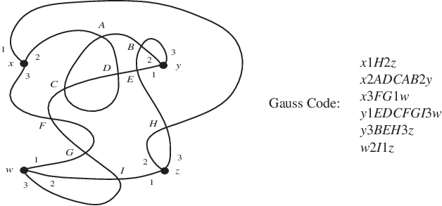
One motivation for the study of virtual spatial graphs comes from the Gauss code of a diagram for a spatial graph. Gauss codes for knot diagrams have a long history, and can be generalized to diagrams of any graph. The Gauss code simply records the sequence of (labeled) crossings along each edge of the graph, so abstractly the Gauss code is just a set of sequences of symbols from some alphabet so that each symbol appears twice in the set. Traditionally, the Gauss code is associated with an immersion of a closed curve (or graph) in the plane, so we begin by looking at the shadow of our graph diagram, where the over/under information at the crossings is ignored. Figure 6 illustrates how we write down the Gauss code for such a shadow.
 |
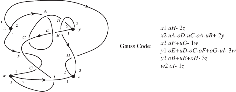
To get the Gauss code for the original diagram, we can augment the Gauss code for its shadow by recording whether each crossing is an over-crossing (o) or an under-crossing (u). If the graph is directed (i.e. the edges are oriented), we can also label each crossing by its sign, positive (+) or negative (-). Figure 7 shows the Gauss code for a directed graph diagram. (Clearly, a Gauss code must have the two occurrences of each symbol labeled with the same sign, and opposite over/under information.)
 |
It is often convenient to look at Gauss codes diagrammatically, using Gauss diagrams or arrow diagrams. In these diagrams, we select a planar immersion of the graph, with the order of the edges at each vertex specified by the Gauss code, label points along the edges according to the crossing sequences of the Gauss code, and then draw an arrow between each pair of occurrences of a label. The arrow is oriented from the undercrossing edge to the overcrossing edge, and is labeled with the sign of the crossing. Once the arrows are drawn, the labels on the edges are redundant, and can be removed. Some examples are shown in Figure 8.
 |
In the case of knots, there is an obvious immersion of the underlying graph - the standard embedding of a circle in the plane. For spatial graphs, the situation is more complicated. In general, there is no canonical choice for the “simplest” immersion of the graph, though generally we will try to minimize the number of crossings. But even if the underlying graph has a planar embedding, the order of the edges at the vertices may prevent us from using it, as in the third example in Figure 8. So the Gauss diagram may have additional crossings, which we simply ignore. Nevertheless, the Gauss diagram is a useful tool for understanding the effects of Reidemeister moves on Gauss codes.
The classical Reidemeister moves (I) - (V) for spatial graphs induce corresponding moves (i) - (v) on Gauss diagrams, shown in Figure 9. So if spatial graphs and are equivalent modulo the Reidemeister moves (I) - (V), then their Gauss diagrams and are equivalent modulo moves (i) - (v).
 |
However, the correspondence between equivalence classes of classical spatial graphs and equivalence classes of Gauss codes (or Gauss diagrams) is not bijective. Even when we are considering only shadows, not all Gauss codes can be realized by the shadow of some graph diagram - those that can be are called realizable or planar codes. An important problem in the study of Gauss codes is to find algorithms for determining whether a Gauss code is realizable. For closed curves, there are several algorithms [1, 2, 10]; the authors have generalized these methods to general graphs [3].
Virtual graph diagrams also have Gauss codes, produced in exactly the same way, except that virtual crossings are ignored (hence we say that they are not “real” crossings). One motivation for studying virtual graph diagrams is that they allow us to realize the “unrealizable” Gauss codes.
Theorem 1
Every Gauss code can be realized as the code for a virtual graph diagram.
Proof: We begin by embedding small neighborhoods of the vertices and the crossings in the plane, with the crossings decorated by orientation and over/under information. The rest of the diagram consists of arcs between the vertices and crossings, and the Gauss code determines the endpoints and orientations of these arcs. Simply draw in any collection of arcs with the desired endpoints, putting in virtual crossings wherever the arcs cross. The result is a virtual graph diagram with the desired Gauss code.
Remark: This proof will most likely not yield the “best” virtual graph diagram. It would be interesting (though undoubtedly difficult) to find an algorithm to produce a virtual graph diagram from a Gauss code with a minimal number of virtual crossings. Presumably, finding this minimal number, the virtual crossing number would be as difficult as finding the classical crossing number of a knot or graph diagram.
So now we want to ask whether the correspondence between virtual graph diagrams (modulo moves (I) - (V) and (I*) - (V*)) and Gauss diagrams (modulo moves (i) - (v)) is a bijection. In fact, we would like to define virtual spatial graphs as simply equivalence classes of abstract Gauss codes modulo moves (i) - (v). However, while every virtual graph diagram has a well-defined Gauss code, it is possible for different diagrams to have the same Gauss code, so the inverse map may not be well-defined. To show that this definition of a virtual spatial graph is the same as our original one, we need to show that two virtual graphs with the same Gauss code are virtually equivalent.
Remark: We can now see why the moves in Figure 5 are forbidden. While moves (I*) - (V*) do not affect the Gauss code, moves (VI*) - (VIII*) do change the Gauss code. Moves (VI*) and (VII*) change the order of the edges around a vertex, while move (VIII*) changes the order of two crossings along an edge. Allowing these moves would force us to expand our list of moves on Gauss codes.
Theorem 2
If two virtual graph diagrams have the same Gauss code, then they are virtually equivalent.
Proof: Our proof follows the argument of the analogous theorem for virtual knots [5]. Assume that and are two virtual graph diagrams with the same Gauss codes, so they have the same classical crossings, with the same local orientations and over/under behavior. By an isotopy, we can assume that these classical crossings are in the same positions in the plane, and that a small neighborhood of the crossings is the same in both diagrams. The arcs connecting these real crossings in each diagram contain only virtual crossings. Say that the crossings and are connected by the arc in and in . Since and have the same endpoints, and have only virtual crossings, may be moved to by virtual local moves (i.e. moves (I*) - (V*)) which do not change the Gauss code. Doing this in turn with every arc in results in a virtual equivalence between and , and completes the proof.
Corollary 1
If a virtual graph diagram has a Gauss code which is realizable, then it is virtually equivalent to a classical graph diagram.
We have not addressed the important question of whether the theory of classical spatial graphs is a proper subset of the theory of virtual spatial graphs, though we conjecture that it is.
Conjecture 1
If two classical spatial graphs are virtually equivalent, then they are classically equivalent.
The corresponding result for virtual knots depends on the fact that the knot quandle (plus longitudes) is a complete knot invariant [5]. While the quandle can be generalized to spatial graphs (both virtual and classical, as we will see in the next section), it is not nearly so powerful. So it is not yet clear how to prove this conjecture in the broader context of spatial graphs.
2.3 Forbidden Moves
If we allow the forbidden moves in Figure 5, then many more virtual graph diagrams become equivalent. In the case of knots, allowing move (VIII*) trivializes the theory, and all virtual knots become trivial [5, 8]. However, when we look at virtual links or virtual graph diagrams, the effect is not quite so drastic - there are some properties which are not trivialized by the forbidden moves (see Proposition 2 in Section 3.1). In this section we will briefly comment on the effects of allowing the forbidden moves.
Proposition 1
Say that is a virtual graph diagram with Gauss diagram . Order the edges of , and let be the set of arrows in with their tail on edge and their head on edge . If we allow move (VIII*) along with the moves for virtual rigid vertex isotopy (moves (I) - (V) and (I*) - (V*)), then we can transform (and hence ) such that:
- 1.
Every arrow of has its endpoints on distinct edges of the graph, so is empty.
- 2.
The arrows in are parallel and adjacent along both edges and , and all have the same sign.
If we also allow moves (VI), (VI*) and (VII*) (so we allow pliable vertex isotopy), then we can also ensure that:
- 1.
has any desired ordering of the edges at each vertex.
- 2.
is empty whenever edges and are adjacent (i.e. are incident to the same vertex).
Proof: First, we will consider the effect of allowing the forbidden move (VIII*). Nelson [8] proves that, in terms of Gauss diagrams, the move (VIII*) allows us move the head or tail of an arrow past the head or tail of an adjacent arrow (on the same edge). This means that any arrow in the Gauss diagram of a graph which has its head and tail on the same edge can be moved until the head and tail are adjacent, and then erased by move (i). So we can transform the Gauss diagram until is empty for every edge .
Similarly, moving arrows past each other allows us to make all the arrows in parallel and adjacent. If any pair of arrow in this set have opposite signs, then they cancel each other by move (ii). So the remaining arrows all have the same sign.
If, in addition, we allow move (VII*) (and therefore move (VI*)), then we can transpose two neighboring edges around any vertex. If two edges and are adjacent at vertex , then we can apply move (VII*) so that they are consecutive in the ordering of the edges around . Using move (VIII*), we can move any arrows in until there are no other arrows between their endpoints and vertex . Then we can use move (VI) (pliable vertex isotopy) to remove these arrows, leaving empty. After removing all these edges, we can once again use move (VII*) to get any desired ordering of the edges around each vertex.
Question 1
What is the equivalence relation on virtual graph diagrams (or their Gauss diagrams) generated by allowing move (VI*), but not move (VII*)? What if we allow (VI*) and (VIII*)?
3 Invariants of Virtual Spatial Graphs
3.1 The collection of virtual knots and links T(G)
In view of the large body of work on invariants of knots and links, a natural place to begin looking for invariants of spatial graphs, or virtual spatial graphs, is among the knots and links contained within the graph diagram. In particular, we are interested in whether individual cycles of the graph are knotted, and whether disjoint cycles (cycles which do not share any edges or vertices) are linked.
To formalize this, Kauffman [6] introduced a topological invariant of a spatial graph (i.e. an invariant of pliable vertex isotopy) defined as the collection of all knots and links formed by a local replacement at each vertex of the graph. Each local replacement joins two of the edges incident to the vertex and leaves the other edges as free ends (i.e. creates new vertices of degree one at the end of each of the other edges). Figure 10 shows the possible replacements for vertices of degree 3, 4 and 5.
 |
Choosing a replacement at each vertex of a graph creates a link (after erasing all unknotted arcs). is the collection of all links for all possible choices of replacements. Kauffman showed that is a pliable vertex isotopy invariant of [6].
For virtual graphs, we can define in exactly the same way, except that it is now a collection of virtual links. Kauffman’s proof easily generalizes to show that is also an invariant of virtual pliable vertex isotopy - in fact, is invariant under all our moves except for move (VIII*) (including the forbidden moves (VI*) and (VII*)). Figure 11 gives examples of for some virtual spatial graphs. It is worth observing that, since the trefoil knot with a single virtual crossing is not equivalent to a classical knot (as can be seen using the Jones polynomial), the third example on the left is a virtual spatial graph which is not equivalent to a classical spatial graph.
 |
Once we have defined , we can obtain invariants of the virtual graph diagram by applying common knot and link invariants to the elements of . For example, we can compute the pairwise linking numbers for all the links in by using the Gauss formula ((number of positive crossings) - (number of negative crossings)). If the links are virtual, these linking numbers may not be integers, but they are still invariant under all the classical and virtual Reidemeister moves. In fact, the Gauss formula is also invariant under the forbidden moves (VI*), (VII*) and (VIII*). For example, the two graphs on the right in Figure 11 have links in with different linking numbers, and so are inequivalent, even allowing the forbidden moves. This shows that the forbidden moves do not trivialize virtual graph theory, as they do virtual knot theory.
Proposition 2
There are virtual graph diagrams which are not equivalent modulo the forbidden moves.
3.2 Fundamental group
The fundamental group of a classical knot or spatial graph is the fundamental group of its complement in . Given a diagram for the knot or graph, this group can be given a presentation, the Wirtinger presentation, involving one generator for each arc in the diagram and one relation for each crossing or vertex, as shown in Figure 12. In the relation at the crossing, changing the direction of an edge interchanges the corresponding generator in the word with its inverse.
 |
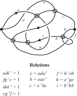
Kauffman [5] defined the fundamental group of a virtual knot by constructing a presentation from a diagram using a generator for each arc between classical crossings, and a relation at each classical crossing. We will define the fundamental group of a virtual spatial graph in the same way, by writing down a presentation with one generator for each arc between classical crossings (or vertices), and relations at each classical crossing or vertex (as shown in Figure 12). An example is shown in Figure 13.
 |
It is easy to check that the fundamental group is invariant under moves (I) - (VI) in Figure 2 (so it is an invariant of spatial graphs up to pliable vertex isotopy). In fact, for a classical spatial graph, this is exactly the same as the classical fundamental group. It is also easy to see that moves (I*) - (V*) in Figure 4 do not change any of the generators or relations, and so the fundamental group is an invariant of virtual spatial graphs. However, all three of the forbidden moves in Figure 5 do change the fundamental group - in particular, moves (VI*) and (VII*) change the relation at a vertex.
3.3 Virtual Graph Quandle
The quandle is a combinatorial knot invariant that was generalized to virtual knots by Kauffman [5], and strengthed by Manturov [7]. Modifying Manturov’s approach, we can construct a similar invariant for virtual spatial graphs, though for general graphs this invariant is less potent than in the case of knots.
Let be a set with one symbol for each arc in a diagram of . Further, let have an operation , an involution , and an invertible function . Construct the set of all words in the elements of using , and .
The virtual graph quandle , an invariant of the virtual spatial graph , is formed from by quotienting out the relations listed below. Following each relation, we note the Reidemeister move(s) that require that relation. To encode information about the diagram, we identify edge labels so that the arcs meeting in a crossing are labeled as in Figure 14.
 |
In addition, we require that all arcs meeting in a vertex be labeled as in Figure 15. That is, we identify the labels of two arcs entering the vertex, and we identify the label of an arc entering the vertex with the bar of the label of an arc leaving the vertex. This restriction at the vertices is needed to ensure invariance under move (IV).
 |
The first three relations are necessary for invariance under Reidemeister moves on the edges of , and are the same as the relations needed for the knot quandle.
| (I) | ||||
| (II) | ||||
| (III) |
We now need to add relations to give invariance under classical Reidemeister moves involving a vertex. Let gcd(), where is the valence of vertex .
| (IV) | ||||
| (IV) | ||||
| (V),(VI) | ||||
| (V),(VI) |
The following relations ensure invariance under the virtual Reidemeister moves. Notice that due to the labeling rule of Figure 14, is already invariant under moves (I*), (II*), and (III*).
| (IV*) | ||||
| (V*) | ||||
| (V*) |
Figure 16 demonstrates the invariance of under Reidemeister move IV. For the left side, we use to show invariance, and for the right, to show that the vertex relation is still satisfied. Invariance under the other Reidemeister moves can be checked in a similar manner. Figure 17 depicts two virtual spatial graphs that are distinguished by their quandles.
 |
 |
3.4 Yamada polynomial
Yamada introduced a polynomial invariant of spatial graphs in [11]. In this section we will review the definition of this invariant, and show that it can be extended to an invariant of virtual spatial graphs.
Yamada’s polynomial for an undirected graph can be defined combinatorially using skein relations as the unique polynomial which satisfies the following formulas:
- 1.
- 2.
, where is a nonloop edge in , is the result of deleting , and is the result of contracting .
- 3.
, where denotes disjoint union.
- 4.
, where is the graph obtained by joining and at any single vertex.
- 5.
, where is the -leafed bouquet of circles and . In particular, if is a single vertex, .
- 6.
Using these skein relations, can be computed by reducing the graph to a bouquet of circles. is an invariant of spatial graphs up to regular rigid vertex isotopy, meaning that it is invariant under moves (II), (III) and (IV) in Figure 2, but not moves (I), (V) or (VI) [11]. The behavior of under these moves are shown in Figure 18 (see [11]):
 |
From these formulas we see that we can obtain an invariant of rigid vertex isotopy (invariance under moves (I) - (V)) by defining , where is the smallest power of in . This will still not be invariant under move (VI), however, so it is not an invariant of pliable vertex isotopy.
In the case of virtual spatial graphs we can use exactly the same skein relations to compute and , simply by ignoring virtual crossings. The only difference is that we may end up with a virtual bouquet - a bouquet of circles with only virtual crossings, as in Figure 19.
 |
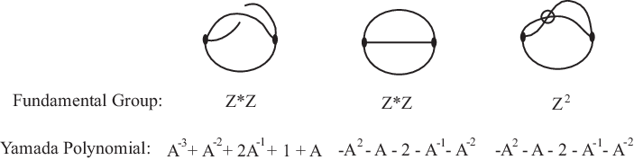
We will simply ignore the virtual crossings. In other words, if is a virtual bouquet of circles, then . Given a planar graph, a planar diagram for the graph is called trivial. It is an open question whether the Yamada polynomial for a non-trivial classical diagram of a planar graph can be the same as the polynomial for the trivial diagram. However, it is easy to find nontrivial virtual graph diagrams of planar graphs with trivial Yamada polynomial. Figure 20 gives three diagrams of the -graph, including the trivial one, together with their fundamental groups and Yamada polynomials. These show that there are non-trivial diagrams with the same fundamental group as the trivial diagram but a different Yamada polynomial, and vice-versa.
 |
References
- [1] de Fraysseix, H. and Ossona de Mendez, P.: On a Characterization of Gauss Codes, Discrete Comput. Geom., v. 22, 1999, pp. 287-295
- [2] Dehn, M.: Über Kombinatorische Topologie, Acta Math. 67, 1936, pp. 123-168
- [3] Fleming, T. and Mellor, B.: Chord Diagrams and Gauss Codes for Graphs, preprint, 2005
- [4] Goda, H.: Bridge index for theta curves in the 3-sphere. Topology Appl., v. 79, 1997, pp. 177-196.
- [5] Kauffman, L.: Virtual Knot Theory, Europ. J. Combinatorics, v. 20, 1999, pp. 663-691
- [6] Kauffman, L.: Invariants of Graphs in Three-Space, Trans. Amer. Math. Soc., v. 311, no. 2, 1989, pp. 697-710
- [7] Manturov, V.: On Invariants of Virtual Links, Acta Appl. Math., v. 72, 2002, pp. 295-309
- [8] Nelson, S.: Unknotting virtual knots with Gauss diagram forbidden moves, J. Knot Theory Ramif., v. 10, no. 6, 2001, pp. 931-935
- [9] Nikkuni, R.: Delta edge-homotopy on theta curves, Math. Proc. Cambridge Philos. Soc., v. 138, 2005, pp. 401-420
- [10] Read, R.C. and Rosenstiehl, P.: On the Gauss Crossing Problem, Colloq. Math. Soc. Janos Bolyai, v. 18, Combinatorics, Keszthely, Hungary, 1976, pp. 843-876
- [11] Yamada, S.: An Invariant of Spatial Graphs, J. Graph Theory, v. 13, no. 5, 1989, pp. 537-551