Minimal surfaces in the roto-translation group with applications to a neuro-biological image completion model
Abstract
We investigate solutions to the minimal surface problem with Dirichlet boundary conditions in the roto-translation group equipped with a subRiemannian metric. By work of G. Citti and A. Sarti, such solutions are amodal completions of occluded visual data when using a model of the first layer of the visual cortex. Using a characterization of smooth minimal surfaces as ruled surfaces, we give a method to compute a minimal spanning surface given fixed boundary data presuming such a surface exists. Moreover, we describe a number of obstructions to existence and uniqueness but also show that under suitable conditions, smooth minimal spanning surfaces with good properties exist. Not only does this provide an explicit realization of the disocclusion process for the neurobiological model, but it also has application to contructing disocclusion algorithms in digital image processing.
keywords
Minimal surfaces, Carnot-Carathéodory spaces, vision, occlusionAMS Subject Classification: 53C17,49Q05,92B05
1 Introduction
The study of minimal and isoperimetric surfaces in Carnot-Carathéodory spaces has recently received a good deal of attention.[2, 3, 6, 7, 8, 9, 18, 17, 21, 20, 12, 24] In the work cited, the various authors explore the existence, uniqueness and properties of minimal and isoperimetric problems, finding that, at least in specific lower dimensional cases, the minimal/isoperimetric surfaces have a rich geometric structure. Moreover, recent work of Citti, Manfredini and Sarti[4, 5] has provided a link between the method by which the brain completes missing visual data in the first layer of the visual cortex (V1) and the solutions to the minimal surface problem in a specific Carnot-Carathéodory space, the roto-translation group, that arises in a mathematical model of the function of V1. In this paper, we denote the roto-translation group by . It is homeomorphic to and we will use as coordinates. Following the construction of Citti and Sarti, we define a Carnot-Carathéodory structure on by distinguishing a horizontal subbundle, , given by the span of the following two vector fields at each point:
These two vector fields bracket generate the tangent bundle and form a distribution of contact planes in this three dimensional space. Placing an inner product on which makes an orthonormal basis for , we have the standard Carnot-Carathéodory distance on :
where is the set of absolutely continuous paths whose derivatives, when they exist, are in .
In this model, a greyscale image, , has a representation in given by
If a portion of the image is occluded in a domain , then Citti and Sarti’s model provides a completion of the occluded region by constructing a minimal spanning surface. More precisely, if is the curve in associated to , then the completion is given finding the minimal surface in that spans , i.e. a minimizer of the perimeter measure. For a surface, , given as a level set of a function , the perimeter is given by
| (1) |
Moreover we know that such minimal surfaces satisfy the following partial differential equation:
In addition to this relationship between the minimal surface problem and a model for biological image reconstruction, Citti and Sarti provide a reinterpretation of a number of existing algorithms for digital inpainting and image completion. In particular, Citti and Sarti[5], and Citti, Manfredini and Sarti[4], examine the variational models of Ambrosio-Masnou[1], and a variant of the Mumford-Shah functional and find that, under suitable interpretation in the roto-translation group model, minimizing these different functionals is equivalent to minimizing the standard Carnot-Carathédory surface area functional given in equation (1). In other words, finding minimizers of these various functionals is equivalent to solving the Carnot-Carathéodory minimal surface problem in the roto-translation group.
In light of this unifying theme in the area of vision and image reconstruction, we explore the minimal surface problem in a class of groups which include the roto-translation group, . Citti and Sarti show the divergence form of the minimal surface equation in and we note that the more general framework of Cheng, Huang, Malchiodi and Yang[3] shows both the divergence form equation and that the smooth minimal surfaces are ruled surfaces. We note that the characterization of minimal surfaces as ruled surfaces has generalizations in Carnot groups with two dimensional horizontal bundles[12] and Martinet-type spaces[6].
In Section 4, we use the basic form of the minimal surface equation to explicitly derive the curves the rule smooth minimal surfaces in the roto-translation group. Specifically, we show that with respect to the Webster-Tanaka connection, , associated to a canonical pseudo-hermitian structure on , the surfaces are foliated by -geodesics which, for fixed and take the form:
Thus, we provide a geometric characterization of smooth minimal surfaces in the roto-translation group which in turn yields an explicit parametrization for every such minimal surface. In constrast to the existing methods of constructing minimal surfaces, which approximate a minimal surface via a diffusion mechanism, we note that this parameterization provides a method for constructing exact solutions to the minimal surface problem.
Second, we turn to understanding the occlusion problem in . As demonstrated in the experimental evidence[5], in the model of V1 given by the roto-translation group, representations of image data in potentially contain different layers of conflicting data due to both modal and amodal completion of the image. In light of this finding, we focus on solving the occlusion problem by finding all possible smooth solutions or partial solutions of the minimal surface problem with a fixed boundary. In Section 6, we develop a test for determining when two points on a given curve can be joined by a -geodesic. We begin with a fixed curve, , which is the boundary of an occluded region of the representation of an image in and is parametrized as . For each point, on , we construct the set of other points on accessible to , denoted . To construct a portion of a smooth minimal surface we simply need construct a function:
where is a connected subset of and so that . We note that to construct a smooth minimal spanning surface, we must have that . For each , this function give a point connected to by a rule. Needless to say, there are numerous possibilities that occur when attempting to construct . In particular, we note that we a guaranteed neither existence nor uniqueness of such a . A key tool in the analysis of is the transversality function given by
where is defined by the equation
To further examine this procedure, we simplify the investigation somewhat and restrict our consideration to curve so that the projection of to is a circle. Under this assumption, we are able to describe a number of different cases ranging from cases where one can always find such a , cases with multiple and cases where no such exists. In each of these cases, we give explicit examples using test image data and give some indication as to the cause of the various pathologies. The examples provide a number of obstruction to the existence and/or uniqueness of smooth minimal spanning surfaces.
On the positive side, after examining these various cases, we present a theorem showing sufficient conditions for when a smooth minimal completion exists.
Theorem 1.1
Let be an intensity function of an image with an occlusion given by a circular region . Further, suppose is the lift of and that the occlusion is completely nondegenerate and occludes no critical points of . If for then there exists a minimal spanning surface of where the projection of each rule of the surface lies in the interior of . Moreover, if for then the projection of this spanning surface to the xy-plane is surjective onto the occluded region.
An occlusion is completely nondegenerate if there are no critical points of on , only a finite number of critical points in the interior of and an angle function can be extended continuously across those critical points (see below for a more precise definition).
We again emphasize that, in such a case, the construction of such a surface is significantly less computationally intensive than the iterative approximative method used by Citti and Sarti[5]. We expect that similar gains can be achieved with respect to the other models mentioned above such as the Ambrosio-Masnou and elastica methods. In this direction, we note that the authors[11] use a discrete version of the method used in this theorem to provide a new algorithm for disocclusion in the context of digital image reconstruction. Moreover, we expect that this method will have application to neurobiology: by explicitly constructing completions of images, we will be able to provide testable hypotheses for neurobiological function of V1.
2 Modeling V1 via the roto-translation group
In this section, we review the basic biological findings describing the function of V1 and describes a mathematical model of V1. Moreover, we describe the connection, provided by Citti and Sarti[5], between minimal surfaces in the model space and solutions to the problem of amodally completing regions of occluded image data.
Over the past several decades, the function and operation of the first layer of the visual cortex, V1, has become increasingly clear. Early research showed that V1 contains so-called simple cells that are sensitive to, among other things, brightness gradients with a particular orientation. These cells are arranged in columns sharing the same orientation preference[14, 15] and the columns are arranged in hypercolumns which represent all possible orientations. This view was further explored and modeled mathematically,[13, 23] where the authors modeled the hypercolumnar cell structure using a contact manifold. The contact model is based on a simplifying assumption that treats each column as a point, ignoring the column structure to focus on the hypercolumn structure. Mathematically, they use the manifold to model the hypercolumn structure by placing a circle of directions above each point . Each point represents a column of cells associated to an point of retinal data, all of which are attuned to the orientation give by the angle . See figure 1 for a schematic of the hypercolumnar structure.

Early assumptions that cortical connectivity should run mostly vertically along the hypercolumns and be severely restricted in horizontal directions, while supported by some research, was contradicted by later evidence which showed that there is “long range horizontal” connectivity in the cortex. These experiments (see for example, Gilbert et al[10]) indicated that horizontal connections are made between cells in different hypercolumns of similar orientation preference. Moreover, experimental evidence showed that there is a stronger preference for communication between cells of not only similar orientation preference but for ones that lie (roughly) along the axis corresponding to the shared orientation. In other words, using the notation of the above model, if and are points in different hypercolumns with the same angle preference , communication between the cells is preferred if the direction corresponds with the direction of the vector from to in . This evidence points towards a geometric structure in this layer where communication between adjacent cells is allowable in certain directions, vertically and between cells in different hypercolumns of similar orientation sensitivity, and vastly restricted in all other directions. This type of situation has been studied in a variety of settings including, for example, control theoretic problems where the degrees of freedom at a particular point are restricted.
Petitot and Tondut[23, 22] incorporate the these biological findings into their model by introducing a contact structure on via the one form and introduce a sub-Riemannian metric associated to the contact two-plane distribution to encode the geometry of the model of V1. The plane field given by the kernel of , , corresponds to the space of allowable directions at each point. Notice that these are precisely the vertical direction and the direction which links cells in different hypercolumns with the same value. Citti and Sarti[5] use the following explicit realization of the roto-translation group, :
- •
is diffeomorphic to with coordinates .
- •
The following three vector fields span the tangent space at each point:
(2) We note that and .
- •
For an image , its representation, , in is given by where and is given by
We note that this is an explicit realization of the model described above and matches with the biological evidence concerning horizontal connectivity. The contact subbundle in this presentation is simply . It is a direct calculation that this subbundle gives a contact structure and, placing an inner product on this subbundle making orthonormal, we have a standard sub-Riemannian metric on (see the next section for a precise definition). One of the main contributions of Citti and Sarti’s adaptation of the cortical model is the use of an explicit lifting function that transforms retinal data into a surface in the cortex and allows direct use of the Carnot-Carathéodory structure.
To explore this further, we investigate the application of the model to an image. Using the representation above, we see that the direction given by the angle points in a direction perpendicular to the gradient of , i.e. a direction tangent to the level sets of . Thus, if nearby points have the same intensity and thereby lie on the same level sets of , their representations will be the same. As denotes a position in a hypercolumn of cells over the point , this echoes the biological finding horizontal communication occurs between cells of similar orientation specificity and the property that the representation respects level lines reflects the biological principle that communication between point and is permitted if points in the same direction as the vector from to . In figure 2, we give a schematic of lifting a simple image to . Represented are two layers of cells of similar orientation preference but different hypercolumns and two sections of the image that could plausibly be lifted to those layers.

Citti, Sarti and Manfredini[4] provide a link between mean curvature flow in Riemannian approximates of the sub-Riemannian space and the celebrated Mumford-Shah functional. Further, Citti and Sarti[5] provided a link between the flow mechanism and several other models including elastica methods[19] and the Ambrosio-Masnou model[1]. Moreover, they showed that surfaces that were asymptotically stationary under the flows in the Riemannian approximates to are minimal surfaces in the sub-Riemannian roto-translation group. As discussed in the introduction, minimal surfaces in Carnot-Carathéodory spaces have been examined in some generality[7, 8, 12] as well as in more restricted settings.[2, 3, 9, 20, 21]
Citti and Sarti[5] use the model of V1 to investigate the problem of amodally filling in an image when a portion of the image is missing due to occlusion or some other factor. To use the model, Citti and Sarti took image data with a portion deleted and used an approximation of the flow described above to find a minimal spanning surface that “fills” the hole in the image. In other words, they find solutions to the minimal surface problem subject to Dirichlet boundary conditions. In the next sections, we will examine the minimal surface problem in the setting of a class of sub-Riemannian spaces which include the roto-translation group. The main goal of this paper is to provide a description of such minimal surfaces and to describe method by which they can be constructed in particularly a simple manner.
3 Notation
In this section, we fix the basic notation used throughout the paper. Let be a topologically three dimensional one step graded Lie group. In other words, the Lie algebra of left invariant vector fields splits as
Moreover, we assume the following
- •
is equipped with a Riemannian metric , which we sometimes denote in inner product notation by and which makes the grading orthogonal.
- •
is the Levi-Civita connection associated to
- •
Assumption 1: is said to satisfy assumption 1 if
- •
We define a Carnot-Carathéodory distance on by
where is the set of all absolutely continuous paths that, where their derivatives are defined, have .
We note that if is nilpotent, then is known as a Carnot group. We review two special examples.
Example 3.1
The Heisenberg group. The topologically three dimensional Heisenberg group, , is one of the simplest nonabelian nilpotent Lie groups. As a smooth manifold, it is diffeomorphic to . Using the terminology above, we have the Lie algebra given as
with and where there is a single nontrivial bracket operation, . We note that, as is nilpotent, it is a Carnot group.
Example 3.2
The Roto-Translation group. As the roto-translation group, , appears centrally in the model of visual processing in V1, we review its abstract structure. As a smooth manifold, it is diffeomorphic to and, using the terminology above, we have the Lie algebra given as
with and where we have the following nontrivial bracket operations, . Equation (2) in section 2 give a particular presentation of . We note that is not a Carnot group as it is not nilpotent.
Given a submanifold , the sub-Riemannian geometry of is determined by the horizontal normal to , , which is simply the projection of the Riemannian normal, , to , the first layer of the grading. Explicitly, if is a left invariant orthonormal basis of with and is given as a level set then,
We also define the unit horizontal normal:
Minimal surfaces in Carnot-Carathéodory spaces have been investigated in a number of settings[2, 3, 7, 8, 9, 21, 20, 12]. In particular, Danielli, Garofalo and Nheieu[7] show that a hypersurface in a Carnot group satisfy the following minimal surface equation:
where is the horizontal divergence operator on . As shown in the next two sections, this equation also characterizes minimal surfaces in the class of groups described above which satisfy assumption 1.
4 Minimal surfaces in
Lemma 4.1.
If satisfies assumption 1, i.e.
| (3) |
then there exists a global strictly pseudoconvex pseudohermitian structure with the following properties
- •
is the contact distribution for .
- •
is spanned by the characteristic vector field for .
- •
The Levi metric agrees with on and is conformal with constant scaling factor to on .
Proof: Let and be a left invariant orthonormal frame for and set . By left invariance and the bracket generating property of , we see that form a global orthonormal frame for . Set to be the dual -form for with respect to this frame. Then clearly and strict pseudoconvexity is immediate as bracket generates at -step. The additional bracket condition (3) implies that . Thus the first two properties hold automatically regardless of which complex structure is chosen for .
Define by and . Next we extend to all of by setting and declaring to be linear over . The Levi metric defined by
then clearly is compatible with in the required fashion.
In this setting, we can now employ the techniques of pseudohermitian and CR geometry. Our key tool is the existence of a canonical connection , derived independently by Webster[26] and Tanaka[25], for any strictly pseudoconvex pseudohermitian geometry. The defining properties of the connection are as follows:
- •
, , , and are all parallel.
- •
for .
- •
for .
Computations using this connection are most easily conducted in the moving frame approach of Cartan, adapted to this setting by Webster [26]. For this technique, we first complexify the contact distribution and define the space of and vector fields to be the and eigenspace of respectively. The vector fields are then spanned by
The vector fields and then form an orthonormal (complex) frame for the complexified tangent space. The dual frame will be denoted by and . We introduce the connection form via the identity
With respect to our frame the Webster-Tanaka connection and Levi metric can be uniquely computed from the following equations[26]:
- •
.
- •
.
- •
.
- •
mod .
The -form is known as the torsion form.
This connection proves well adapted to many geometric problems. For the study of horizontally minimal surfaces we have the following theorem.
Theorem 1.
Suppose is a non-characteristic surface patch in a Carnot group satisfying our structure conditions. The horizontal minimal surface equation for
| (4) |
can be written as
where is the horizontal unit normal. Thus if satisfies (4) then is ruled by horizontal -geodesics.
Proof: The volume form for the Levi metric is given by . By the defining properties of the pseudohermitian structure this is a constant multiple of the Riemannian volume form. From this we immediately see that is parallel for and the divergence operator for agrees with the Riemannian divergencve. Further it f ollows that and so
Now , and form a local orthonormal frame for . A standard formula in Riemannian geometry (see for example Kobayashi[16]) then yields
If is horizontal then the second part of the trace formula vanishes identically by the defining properties of the Webster-Tanaka connection. Using our particular choice of frame we then see that
as the second and third terms vanish because is parallel and the connection is metric respectively. Thus on a non-characteristic, horizontally minimal surface patch we have
| (5) |
everywhere. The integral curves of are therefore -geodesics. But spans the intersection of with . Thus the integral curves of foliate .
Remark 2.
The divergence form of the mimimal surface equation in was first shown by Citti and Sarti[5] (see section 2.9 proposition 3.1 of that paper) but is also a consequence of the more general psuedoherimitian framework of Cheng, Huang, Malchiodi and Yang[3]. We also note that a version of this theorem, showing that smooth minimal surfaces are ruled, was first shown in section 2 of Cheng, Huang, Malchiodi and Yang,[3] again in the more general context of psuedoherimetian manifolds. We include the proof here for completeness and because it facilitates the computations below.
We shall now apply these techniques to the special case to the roto-translation group . Here the underlying manifold is and is defined by setting
and declaring them to be a left-invariant, orthonormal frame for a distribution . The Riemannian structure by defining the transverse vector field,
and declaring it to be unit length and orthogonal to and . The remaining commutation relations can then be explicitly computed as
When we run through the construction of Lemma 4.1 we note that is exactly the Levi metric in this case. The contact form can be explicitly computed as
and the dual to the complex vector field is
Straightforward computations then yield
The first identity also follows from the fact that the pseudohermitian structure was explicitly constructed to ensure that and were orthonormal. Since we can immediately deduce from the 2nd Webster identity that the connection form is pure imaginary. Thus we can deduce that
This implies that for the frame the only non-trivial covariant derivatives are in the direction. By examining the real and imaginary parts of the equation
we see and .
The horizontal -geodesics can be computed explicitly. Consider a curve . Thus
Thus if is a purely horizontal curve, we must have
Under this assumption, if and only if both and are constant. We can then solve the equation
to obtain , .
- •
Case 1: . Set , then
Here , .
- •
Case 2: . Set , then
In the sequel we shall refer to the horizontal -geodesics (and connected subsets of them) as rules.
5 Missing data and amodal completion
We next turn to the problem of filling in missing image data. Image data may be missing for a number of reasons: one object occludes another, the existence of a “blind spot” in the retina or some other physiological failure. In terms of digital image processing, data corruption, noise or object occlusion can de facto create a domain of missing data.
Using the roto-translation model for the hypercolumn structure in V1 described above, image data is lifted to and missing data is filled by solving the minimal surface problem for the given boundary data.[5] Mathematically, if is an open domain where image data is missing, and is the image of under the lift defined in section 2, then we wish to find a minimal surface so that . Moreover, as discussed in the previous two sections, a surface meeting these requirements must satisfy the equation:
where is the unit horizontal normal to . Moreover, by theorem Theorem 1, must be ruled by horizontal -geodesics. For the balance of the paper, we will consider the following problem:
Occlusion problem: Given a smooth curve, , in which is the lift of the boundary of an open domain in , can we find a smooth minimal surface spanning which is ruled by -geodesics?
As referenced in the previous sections, this type of problem has been studied before in a number of sub-Riemannian settings. In addition to the observation that minimal surfaces in some settings are ruled surfaces, there are a number of results further describing the nature of solutions to the minimal surface problem with Dirichlet boundary data. Among these results, it is important to note that, at least in the Heisenberg[20] and Martinet-type spaces[6], there are obstructions to the existence of smooth minimal spanning surfaces, even if the spanned curve has arbitrarily nice behavior. Moreover the second author demonstrates[21] that solutions to the Dirichlet problem for ruled minimal surfaces need not be unique (however, Cheng, Huang, Malchiodi and Yang[3] prove a uniqueness result for surface subject to certain constraints on the characteristic locus). Thus, as the roto-translation group is locally very much like the Heisenberg group, we should expect to see issues with both existence and uniqueness. In light of this suggestive evidence, we present a list of conditions, each stronger than the next, concerning a smooth minimal spanning surface :
- (I)
exists
- (II)
Condition I and any rule connecting two points of projects to a curve in the interior of
- (III)
Condition II and the projection of to is surjective.
- (IV)
Condition III and is a graph over
- (V)
Condition IV and is unique
We note that if condition II is violated, the rules, upon projection, would present potentially conflicting data for points exterior to while if condition IV is violated, there would exist points interior to with conflicting projected image data. Thus, condition III is sufficient to guarantee the existence of a completion of the image data (not just a spanning surface in ) although there may be conflicting data while IV would provide a completion with no conflicting data. However, as, a priori there may be multiple lifts, only condition V would yield a unique completion of the image data.
The evidence cited above and the experimental evidence of multiple simultaneous completions of image data in [5] suggests that we should not expect to be able to satisfy the more stringent requirements. As we develop the machinery to construct such surfaces, however, we will keep each of these conditions in mind.
6 Ruled surfaces in
In this section, we begin the investigation of the existence and properties of minimal ruled spanning surfaces of curves in . As we require the solution to the occlusion problem to be a surface ruled by -geodesics, we first look at the set of points which can be connected to a given point by -geodesics. With this in mind, we make the following definition:
Definition 1.
For a point we define the accessible set to be the collection of points that can be connected to by a single, horizontal -geodesic.
Lemma 6.1.
Given a point , the set of accessible points is given by the implicit equation
Proof: When the connecting -geodesic is a straight line this is immediate. The other case follows easily from the trigonometric identity
| (6) |
The proof of this identity is an easy exercise with the tangent half-angle formulas.
This provides a description of the accessible set of :
Lemma 6.2.
Every accessible set is the image of an embedding of the Mbius strip into .
Proof: We shall give two arguments for this result. One purely geometric, the other more analytic.
From Lemma 6.1 we note that each -slice of projects to a straight line in the -plane of gradient . As increases this line rotates spanning out a helicoid. However since we must identify with and the factor of inside the means that there is an orientation switch at the join. Thus is a non-orientable line over which therefore must be diffeomorphic to a Mbius strip.
A more analytic approach is to consider the -exponential map at restricted to the horizontal distribution. From our explicit description of the horizontal geodesics passing through we note that if then
| (7) |
at least when . When we instead get
| (8) |
If we must therefore have that (with neither being ) and . This later can be summarized as the points and must lie on the same line through the origin with . Therefore the exponential map is bijective from to provided that the sides of the strip are identified via . This provides an explicit embedding of the Mbius strip into with image .
For each point on a curve , may contain many points of or very few. Of most interest to the question of building spanning surfaces are the points where - i.e. the points that only connect to themselves. These points give constraints on the formation of a minimal ruled spanning surface. To help understand these points, we make the following definition:
Definition 2.
Given an embedded curve and a point we define
the points in accessible to . A point such that is called an solitary point of . The solitary points of will be denoted . A point such that is called a Legendrian point of . The Legendrian points of will be denoted . We also define the orthogonal points of , denoted to be where .
As seen in the definition, there are two types of solitary points, the Legendrian points and the non-Legendrian points. We remark that for a Legendrian point , the candidate rule passing through is tangent to the curve and, as in the Heisenberg group[20], one can use this as a starting place for building a ruled minimal spanning surface. the non-orientability of the accessible sets in the roto-translation case means that unlike for the Heisenberg group we cannot deduce that all solitary points are Legendrian. Indeed non-Legendrian solitary points present more of a problem as the candidate rules will be transverse at such a point. To investigate the structure of the set of solitary points further we prove the following lemma.
Lemma 6.3.
For any embedded curve , the set is open.
Proof: If , then intersects only at and does transversely. A small perturbation of the base point will cause a small perturbation of the Mbius strip embedding. As is transverse to , a small perturbation of cannot increase the number of nearby intersections. Away from the Euclidean distance of from can be uniformly bounded below and so a small perturbation will not introduce any distant intersections. Thus curve points sufficiently near to will also be solitary. Clearly they will also be non-Legendrian.
Lemma 6.4.
Suppose is an embedded curve and . Then the map
is surjective.
Proof: This is a topological argument. Suppose is a curve in that projects to the xy-plane bounding a domain . Further suppose there exists not in the image of . Then, there exists a neighborhood of , , so that . By Lemma 6.2, is a Mbius strip. However is orientable. Since , by assumption, cannot enter we see that lies to one side of . However, since , must intersect transversely at . This is a contradiction.
For the occlusion problem we shall work exclusively with curves that occur as the boundary of a smooth, simply connected bounded region lifted by the contour direction field of an intensity function . The boundary is can be viewed as the image of an embedding . Away from critical points of , we can define the lifting function by
where at each point we choose the branch of which makes continuous. We shall that an occlusion is non-degenerate if the number of critical points of lying inside is finite and can be extended continuously across each critical point. The occlusion is completely non-degenerate if there are no critical points on the boundary. Using this function we construct the curve . In addition we define the normal angle function for by
From these we construct the transversality function for ,
From the definitions, it is clear that a non-critical point is Legendrian if and only if , . Likewise is orthogonal if and only if . We record this and another fact in a lemma:
Lemma 6.5.
For any lift associated to a completely non-degenerate occlusion problem,
- (1)
is Legendrian if and only if for some integer .
- (2)
is orthogonal if and only if for some integer .
- (3)
is non-empty.
Proof: For the first item, we note that, by definition, is Legendrian if . Computing, we have
and so, if we assume is Legendrian, we have that, equivalently, or . The second item, concerning orthogonal points, follows in the same way.
The last item follows immediately from the observation that
where is the angle between and . Since the first two terms of the integral are strictly positive we must have taking both positive and negative values. In particular, this implies there are at least two points in where . By the computation at the outset of the proof, these two points are Legendrian points.
Remark 3.
We note that in the proof, we provide a geometric interpretation of : it measures the angle between and .
7 Occluded Disks
For computational reasons, it is useful to restrict attention to curves that are lifts of circles in to the rototranslation group. The lifts we are most interested in come from the direction angles of the contours of an intensity plot which has an ambiguity associated with the choice of orientation. Given a point and a contour passing through this point at angle , it is unclear whether to lift it to or . Accordingly, for a point we shall define its conjugate point to be and frequently consider conjugate lifts and simultaneously.
Any circular lift can be expressed parametrically in standard form as
| (9) |
When is understood, we shall frequently refer to a point of simply by its parameter value with this parametrisation. With this parametrization understood we can simplify the transversality function to
| (10) |
Lemma 7.1.
For a circular lift , the non-trivial part of is given implicitly by
| (11) |
and is given implicitly by
| (12) |
Proof: From Lemma 6.1 we see that if and only if
Applying the trigonometric identity (6) we see that this is equivalent to
The result then follows easily from standard arguments in trigonometry. A virtually identical arguments yields the second part also.
Lemma 7.2.
Conjugation twist-commutes with the exponential map in the sense that.
Corollary 1.
If then . Furthermore the projections to of the connecting rules match precisely.
Therefore when connecting points obtained from lifting intensity plots we need only consider how points in can be connected to either or . We shall write if either of lies inside .
Lemma 7.3.
The Legendrian points of occur precisely where
The orthogonal points of occur precisely where
Proof: Since is parametrized by (9), we can explicitly compute that
For it is then necessary and sufficient that . For the condition becomes . The result follows easily.
Corollary 2.
, .
Corollary 3.
On an implicit plot of all points such that . Any transverse crossing of the leading diagonal occurs at either a Legendrian or an orthogonal point.
Corollary 4.
If and then . Furthermore, the connecting rule projects to the same circle as .
If and then .
With circular lifts, if two points on are known to be connectable then it is a straightforward matter to explicitly describe the connecting rule. If with then the connecting rule must have the parametrisation . Thus we need only solve the matrix equation
| (13) |
where the fact that the points are connectable guarantees the existence of a solution. Elementary methods yield that generically
| (14) |
This of course yields two separate connecting rule segments depending on whether transverses clockwise or anticlockwise.
Lemma 7.4.
If is the circular boundary of a completely nondegenerate occlusion and if , then .
Proof: We may assume, without loss of generality, that , and is parameterized by arclength. If is zero, then we must have that is connected to itself. Thus, there exists a finite speed parametrization so that and is connected to for close to . Using (13), if we let be the radius of the circle connecting to , for a generic choice of , we must have
Assuming that as , then we must have that
As are bounded and , we have that as . However, direct computation shows that
where is the Hessian of . If and the occlusion is completely nondegenerate, then must be bounded on . Thus, cannot tend to zero.
With these initial observations in place, we turn to the task of understanding when minimal spanning surfaces exist. We will investigate such surfaces using the following blueprint (if possible):
- (1)
Construct the function as given in (10).
- (2)
Find all solitary Legendrian points using lemma Lemma 7.3.
- (3)
Starting from a solitary Legendrian points, construct connections between points on to other points on using the implicit equation
and the matrix equation above.
Subject to goal of satisfying conditions II and III from section 5.
As we shall see, any one of these steps and/or goals may be violated. One issue we address first is that it may not always be possible to construct such a surface by connecting points of to other points of . In this case, as discussed above, it is natural to instead connect some (or all) points of to points of .
8 The index of
To construct a minimal spanning surface for we choose the a Legendrian point as a starting place and attempt to build a monotone function such that by following the branch of the implicit plot until we reach the other Legendrian point. If we implicitly differentiate either (11) or (12) with respect to , we see that
In particular, these implicit plots fail to be graphs over the -axis precisely when either or . The presence of such points is a necessary condition for obstructions to the existence of a monotone function . If we have intervals of positive measure where is strictly positive and others where it is strictly negative, then we note that a spanning surface will not be a graph over as the change in sign forces the spanning surface to backtrack locally, violating our goal IV. Generically, even if such points occur we can still follow a branch of the implicit plot and constuct connecting rules, however there will be non-uniqueness issues. This approach will only completely fail if the plot fails to be an embedded curve, which occurs only at points where .
If we can construct a monotone function , then the collection of connecting rules will form a minimal spanning surface for the lift . In practice, there are several types of obstructions to this method.
Of primary importance is the degree of the map . Since connections are made by implicitly solving the equation
| (15) |
the size of the set is intimately related to . For example if then there cannot be any non-Legendrian solitary points as non-zero degree implies is surjective. Likewise, it is clear that
Of course, critical points of add a seperate pathology which influences the number of branches of the implicitly defined function of (15).
For the occlusion problem, the degree of is directly related to the critical point theory of the intensity function . If the occlusion is completely non-degenerate, then there is a well-defined map
The continuous lift is then given by . Hence
To explore this further, we shall suppose that has at most one (nearby) critical point which if it exists is contained in the interior of the occluded region . In this instance it follows from the definitions that
if exists. If there is no critical point in the interior then extends to a continuous function on the interior disc. Standard results in algebraic topology then imply that and so .
Next, we examine various possibilities for the occlusion problem. We will deal primarily with completely nondegenerate curves.
8.1 Case 1: ,
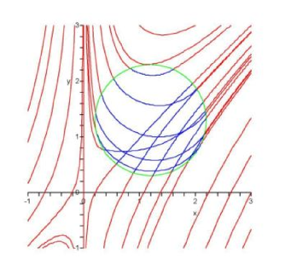
As a basic example, we consider the following example: set the intensity function as whose contour plot looks like an angled cross, see Figure 3.
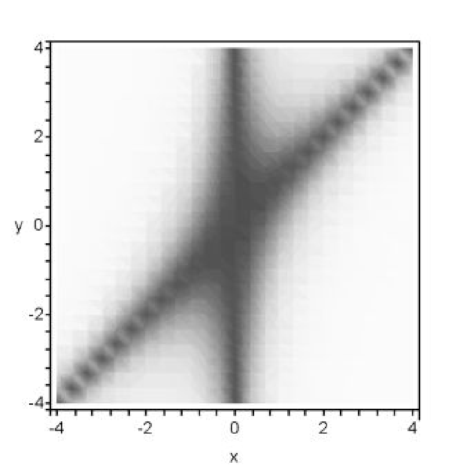
The region to be occluded is , which is over just one branch of the cross. While formally has critical points everywhere along the lines and , we can replace with without altering the underlying contour plot. With this simplification, we have a completely non-degenerate occulsion with no occluded critical points. Thus (and hence surjective onto ). The implicit plot of (15) is shown in Figure 4. In this instance we see that is one-to-one from to and so there is only one branch of (15), which spans the entire range. Moreover, direct calculation shows that for all . The boundary lift has exactly Legendrian points, represented in Figure 4 (b) by the intersection of the curve with the blue lines and . The intersections with the lines and correspond to the orthogonal points.
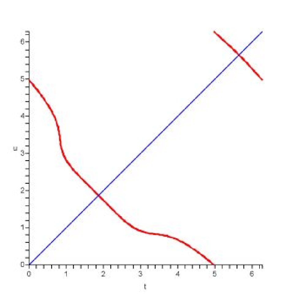
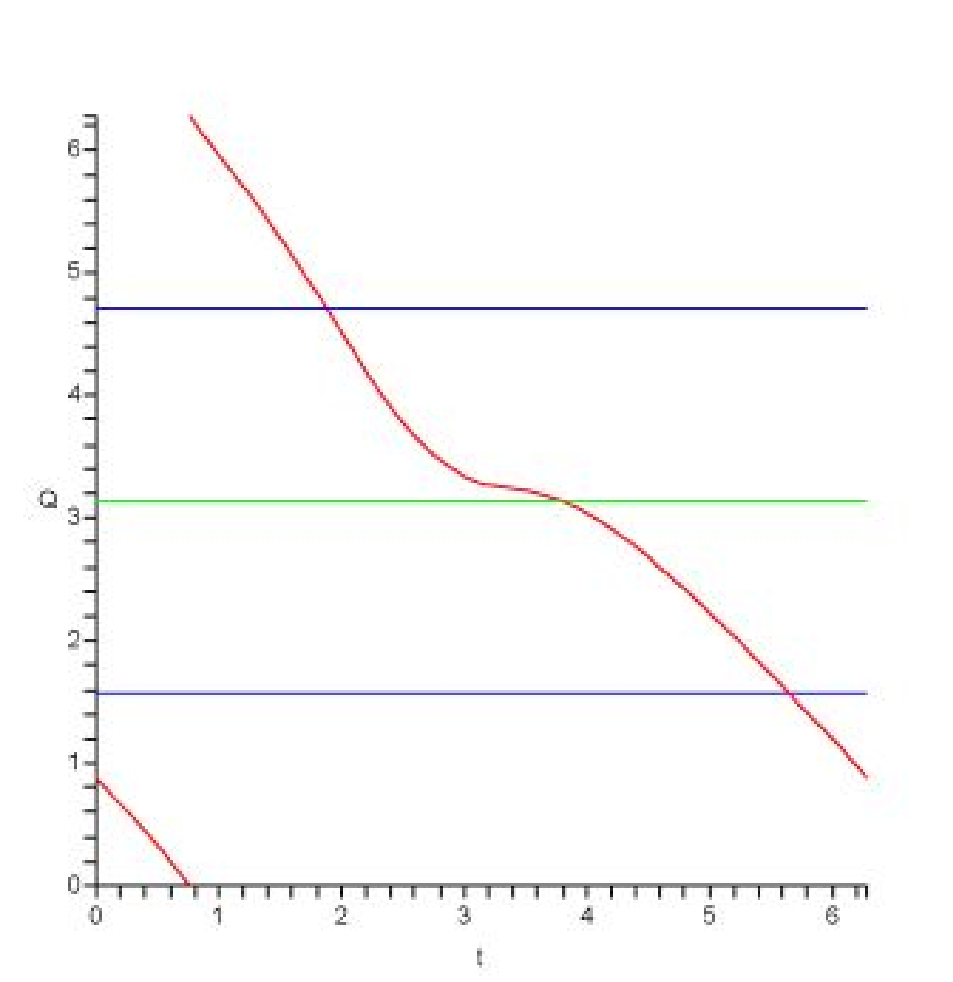
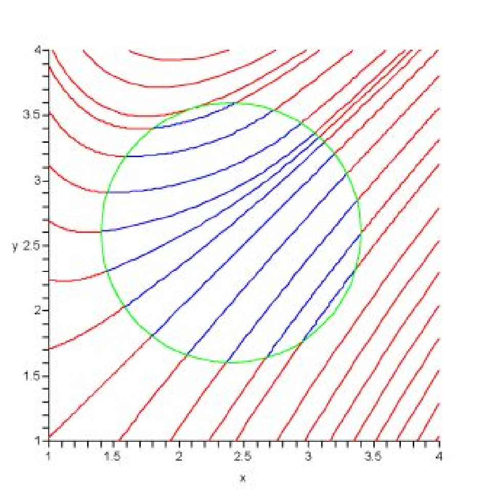
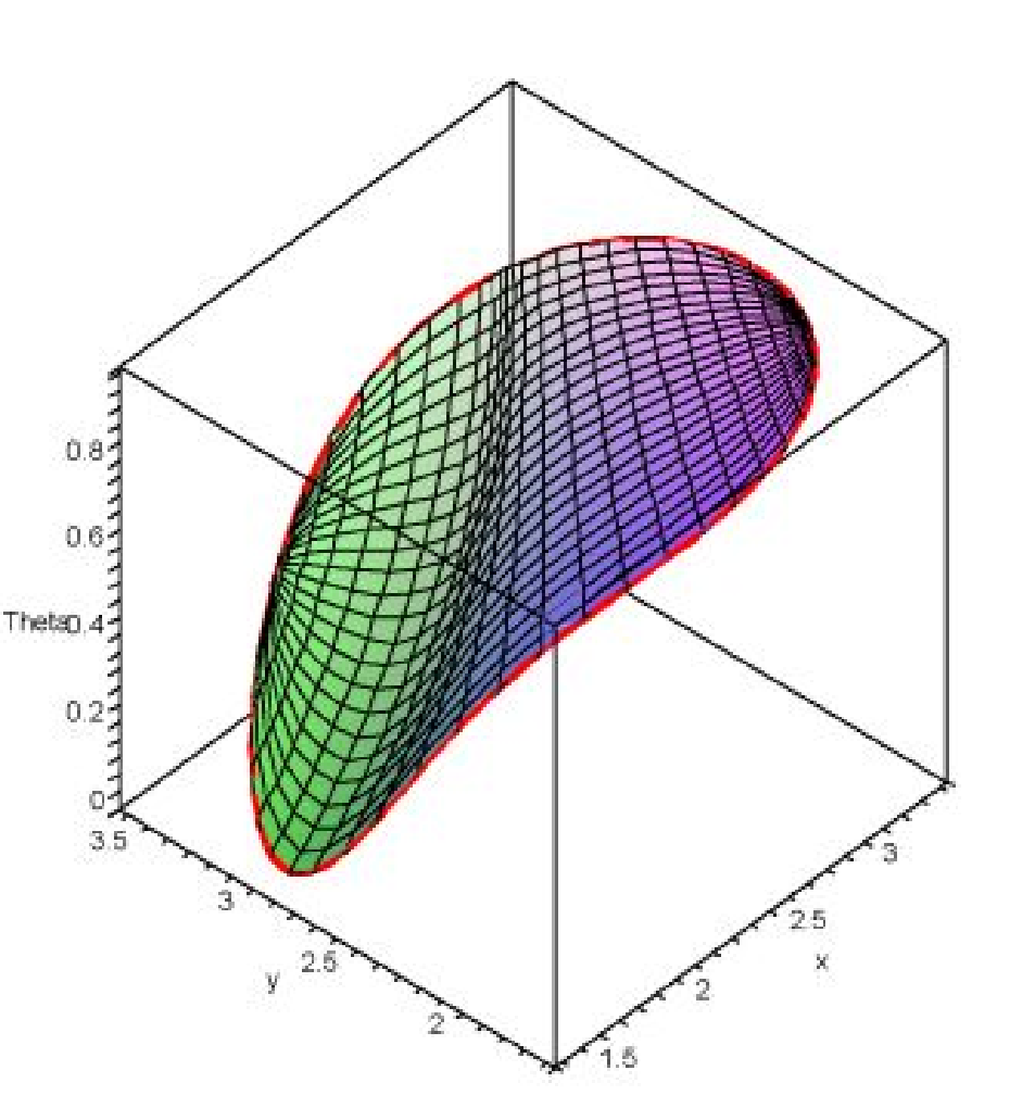
Since Legendrian points can only connect to other Legendrian points (by corollary Corollary 4), we see from the implicit plot of (15) that the Legendrian points for are solitary and correspond to the intersections with the leading diagonal in Figure 4 (a). Thus we can pick either and construct connecting rules by tracing the sole branch of the implicit plot until we reach the other Legendrian point. By symmetry every point on the curve has now been connected to another and we can build a surface ruled by the -geodesic segments that project into the interior of the occluded region. The projections of these segments provide a contour completion through the occluded region. In Figure 4 (c) and (d) we show the full contour completion together with the associated minimal lift in the roto-translation group. We note that it is possible to show that the surface constructed is a graph over the occluded region and hence satisfies condition IV.
8.2 Case 2: , has zeros
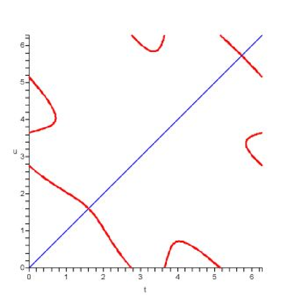
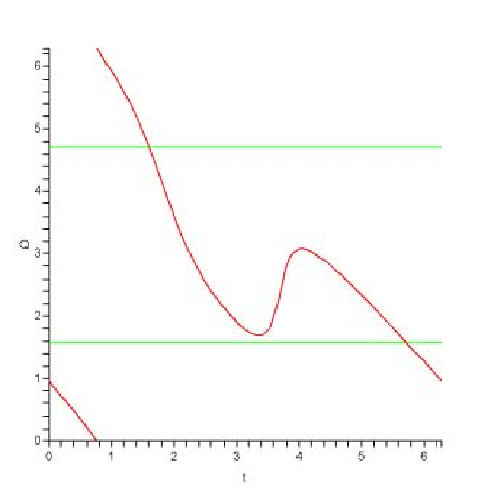
The last example worked so well because not only was , but also because was injective. This was because the directions of the underlying contours were relatively uniform. If we move the occluded region in closer to the centre of the cross, we lose this uniformity and we find that depsite having degree is no longer injective. Examining Figure 5 confirms that there are points where (this can also be confirmed by direct calculation). This is represented by the failure of the implicit plot of (15) to be a graph over either or . When we follow the program laid out earlier for constructing minimal spanning surfaces, we find that some points have multiple connections. The surface then connects to some parts of the curve as a ridge. Note this surface satisfies condition II but not III.
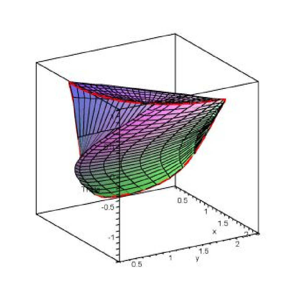
8.3 Case 3:
If then there are possible obstructions to even local existence of spanning surfaces for . This phenomenon occurs due to the presence of non-Legendrian solitary points. Non-Legendrian solitary points do not occur in isolation but as open sets by Lemma 6.3. Since is continuous, the presence of non-Legendrian solitary points implies that the image of is contained in a narrow (width ) band. In particular, this implies that the condition is necessary. In the situation of a single critcal point of being occluded, the index of must be . In other words, we must be occluding a local maximum or minimum.
A simple example is to consider the circular lift
| (16) |
Here everywhere and so every point is orthogonal with outward pointing orientation. The set of that satisfy (15) is therefore empty. Every point is therefore solitary and non-Legendrian and there is no non-characteristic minimal surface that spans even a part of .
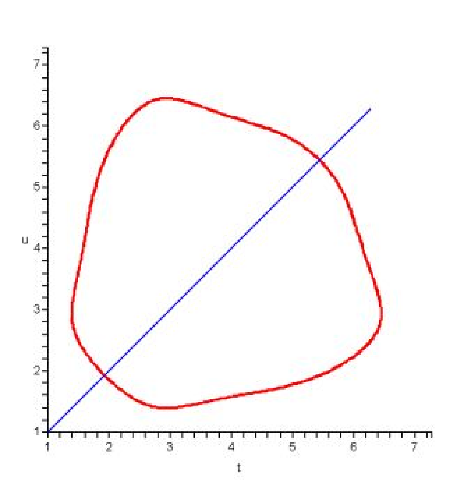
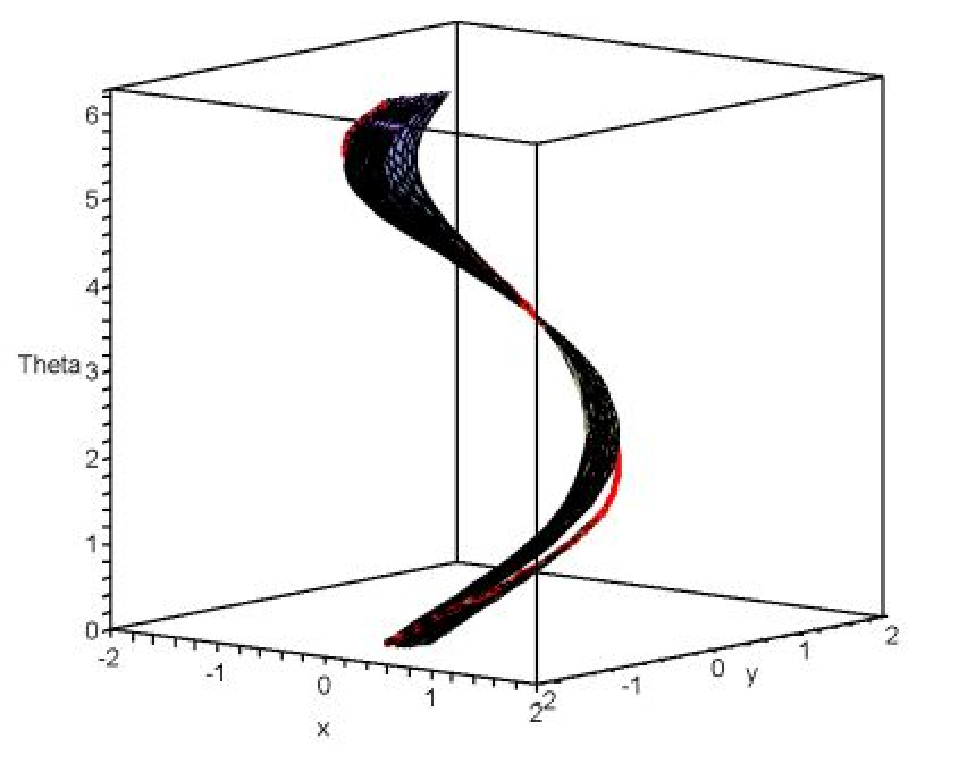
It is clear that the lift (16) cannot occur from an occlusion problem as it would require the vector field to be rotational and hence non-conservative. However gaps in the implicit plot are characteristic of occluded maxima and minima, at least in the absence of symmetry. See Figure 6 for an explicit example where and the circle occludes a local maximum of the function. In figure 6 (a), we see that there are two gaps where there are no connections between and any other point on the curve. The nature of the gap as part of the minimal spanning surface is shown in the remaining graphs.



8.4 Case 4:
When has large degree, the phenomena of overlapping contours and immersed, discontinuous spanning surfaces occurs naturally even when we are considering only rules connecting to itself. In Figure 7 we return to the intensity function , but with the occluded region shifted to have centre and radius . Since we are now occluding the saddle point (of ) at , the degree of is .
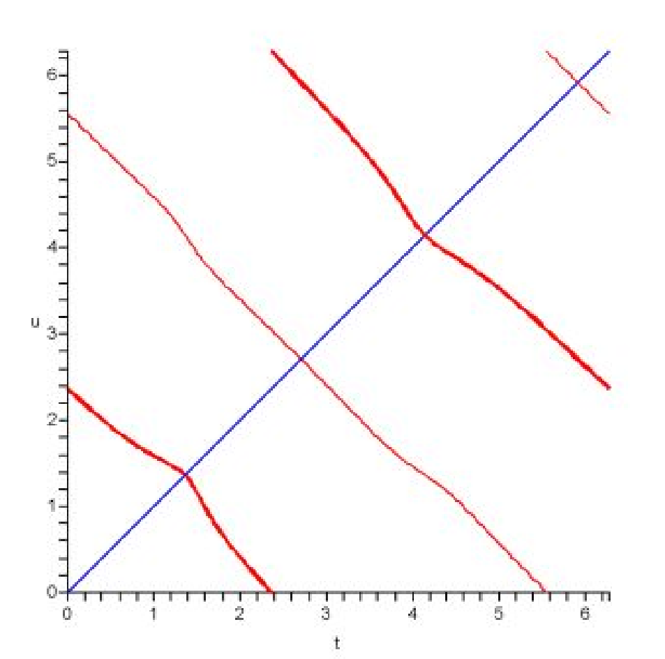
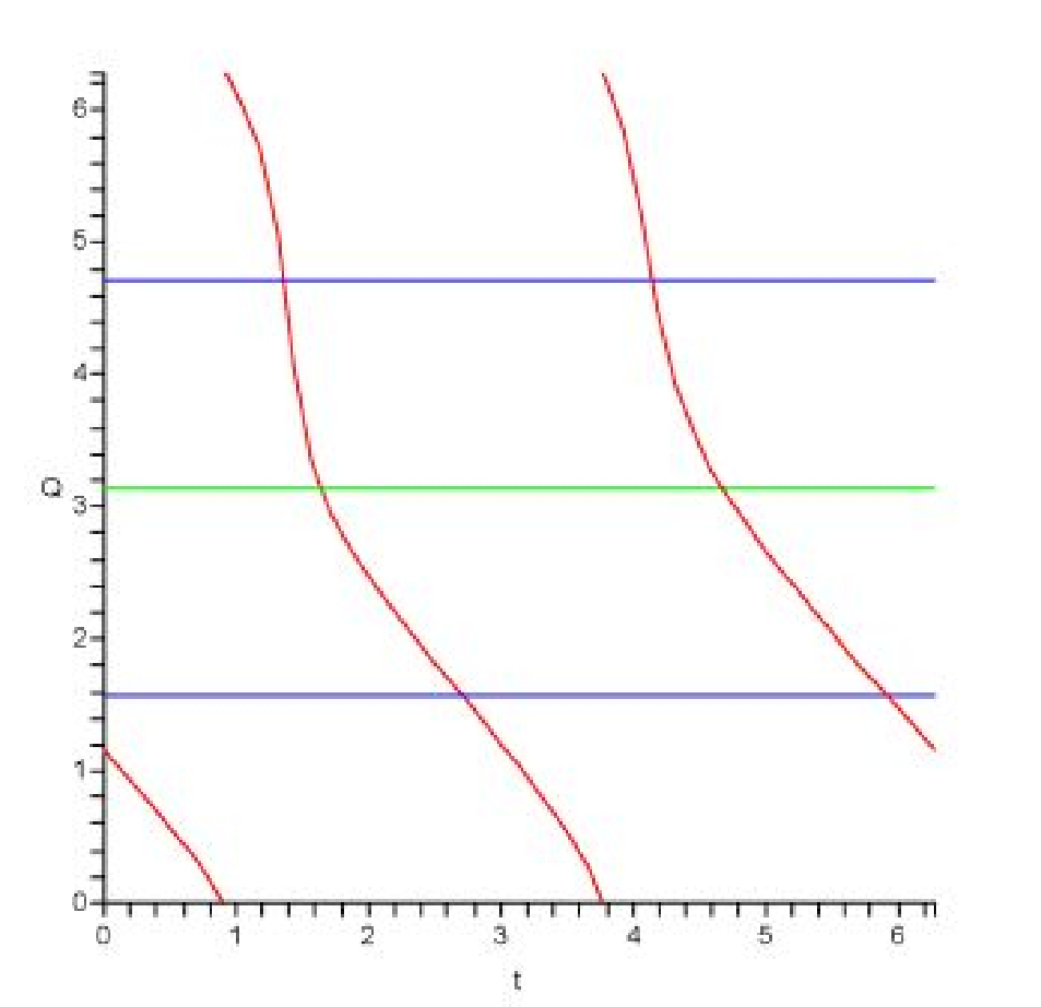
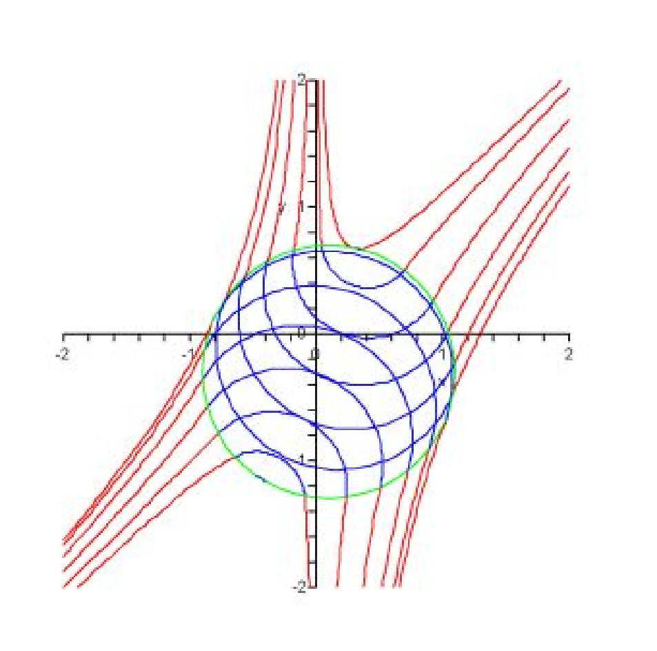
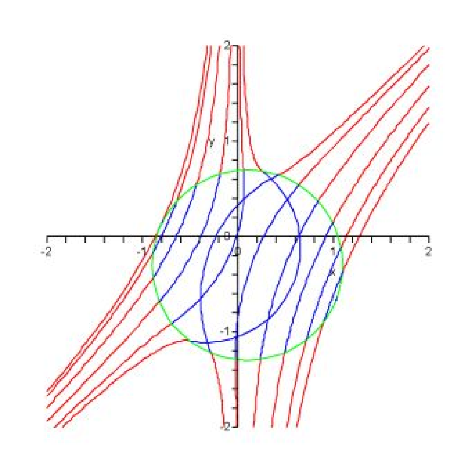
In this instance we see that is now a monotone two-to-one function from to . This corresponds to there now being two branches of the implicit plot of (15) in Figure 7 (a). For convenience of reference we shall refer to the highlighted branch as branch I and the other as branch II. In both contour completions there is overlap as Legendrian points are crossed while transversing the branches.
8.5 Connecting to
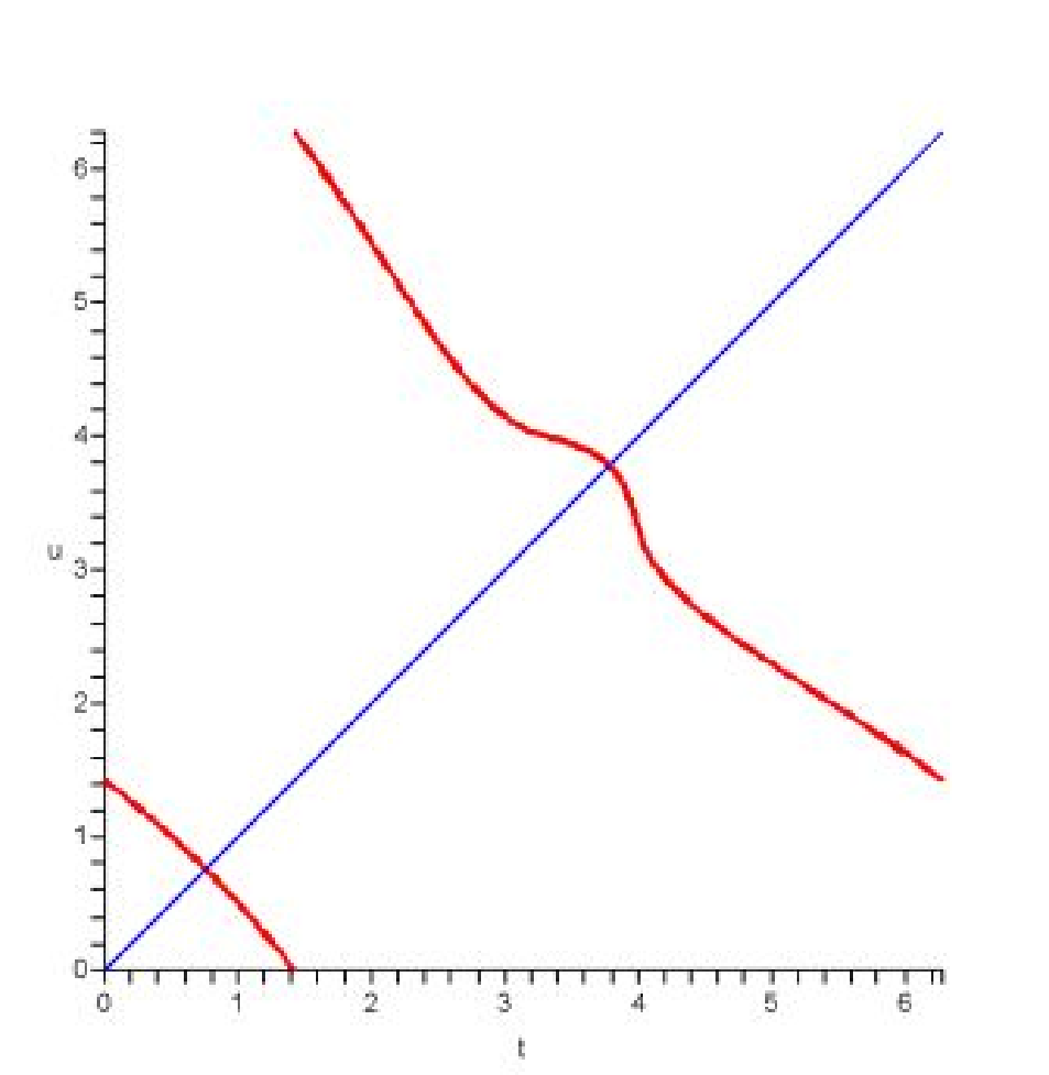
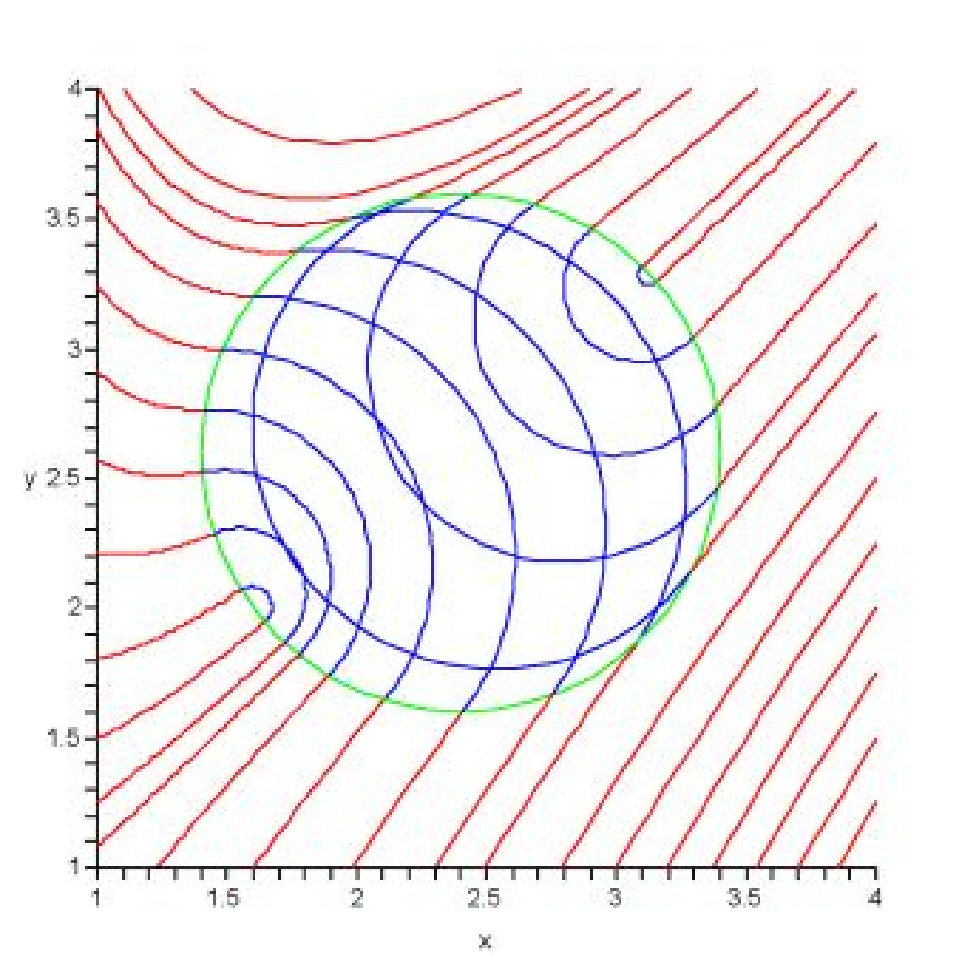
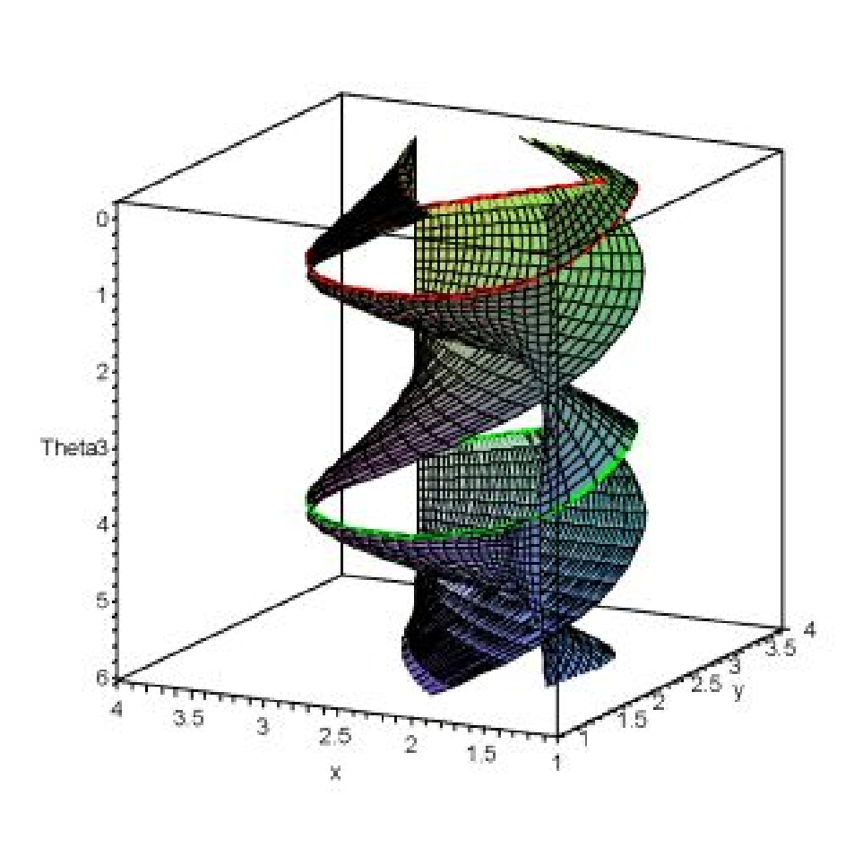
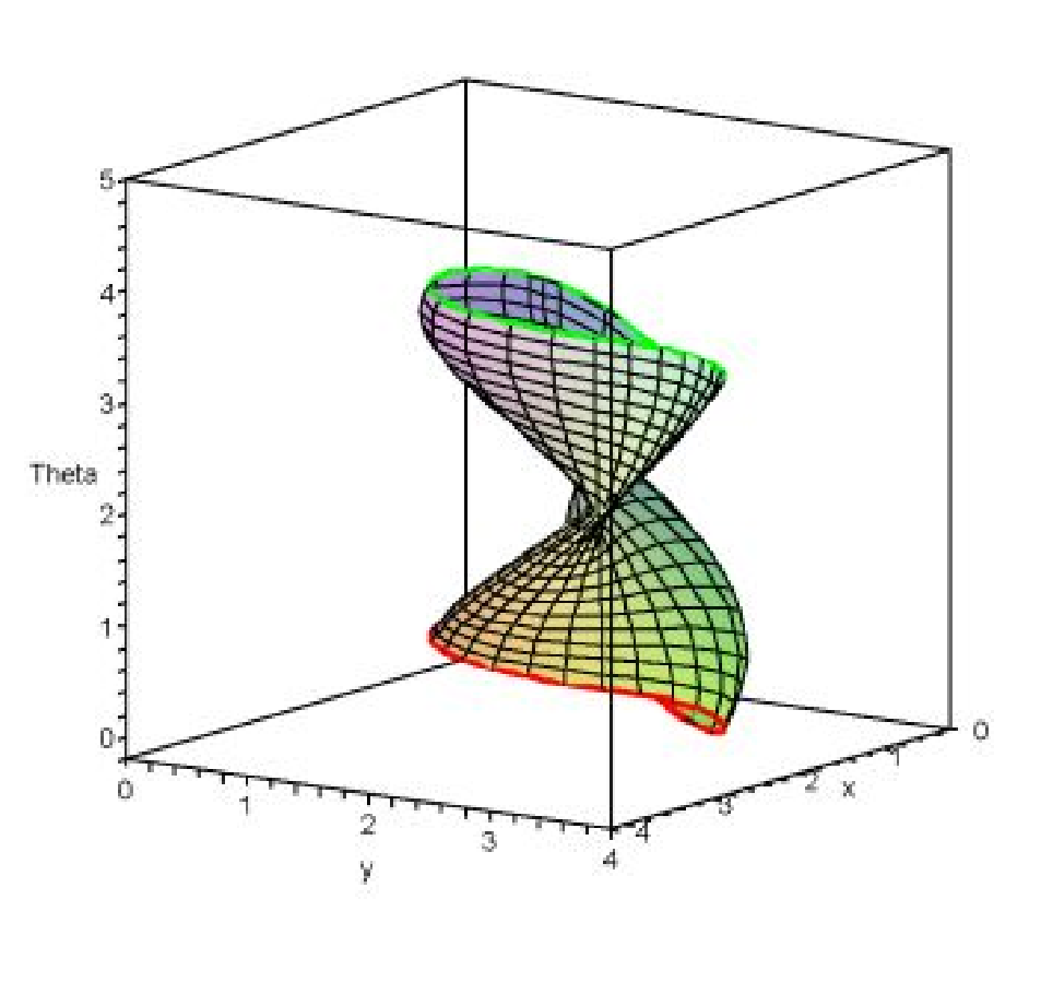
For the problem of visual completion we must consider also rules connecting the lift to its conjugate lift . To illustrate this we return to our original example with the occluded region being the unit disc centred at . We follow the same basic program, but instead focus on the orthogonal points as our start and finish locations. Unfortunately, this introduces a pathology into the construction of our contour completion and minimal spanning surfaces. To progress from one orthogonal point to the other along a branch of the implicit plot of (12) it is necessary to pass through a Legendrian point. The effect of this is to switch which segment of the connecting rules projects to the interior of the occluded region. As is seen in Figure 8 (b) this causes overlaps of the contour completion. If we look at the minimal surface formed from these internal rule segments, in order to completely span we must continue further along the branch until we return to the original orthogonal point. This produces the discontinuous self-intersecting surface of Figure 8 (c) . From the perspective of minimal spanning surfaces, it is more natural to allow rule segments that project outside the occluded region. As is shown in Figure 8 (d), this yields a smooth immersed surface between and , but it still self-intersects.
9 A sufficient condition for effective disocclusion
The examples of the last section point to several general features of the solutions to the occlusion problem. We will now show that under some assumptions on the image function , we can guarantee the existence of a solution to the occlusion problem, ie. a minimal spanning surface satisfying condition III. To do so, we need some preliminary lemmata.
Lemma 9.1.
Let be an intensity function of an image with a completely nondegenerate occlusion given by a circular region . Suppose there exists a minimal spanning surface of the occluded region associated to a monotone function and so that the projection of to is not surjective. Then, one of the rules of the minimal spanning surface is a circle that, when projected to lies entirely inside and is tangent to the boundary of at a Legendrian point.
Proof: We begin with some simple geometric observations. First, if is composed of circles of infinite radius (i.e. straight lines), the projection is trivially surjective. So, we may assume there are some circles in that have finitie radii. Second, let be the circle that bounds the occluded region (as above), oriented counterclockwise, and let be a circle of finite radius connecting two points on that is the projection of a rule of . If is the inward pointing normal to , then let where is the angle (in ) between and at . Then, if connects to , (see figure 9 (a)). Moreover, in the degenerate case where , the circle is tangent to (i.e. is Legendrian) and thus . Since is monotone (and in particular, one to one) and are continuous in , is well defined and, for , is continuous. At points where , may have a jump discontinuity as will switch sign at such points.
By Lemma 6.5, we have that there are at least two Legendrian points and so, by the previous discussion, the function potenitally switches sign as is zero at a Legendrian point. Consider now a circle passing through such a Legendrian point. Then (see figure 9 (b)) if the circle is to lie outside the occluded region, then moving in the direction of the parametrization of , we must have that moves from positive values to negative values. For to change sign, we must have that the inward normal to the rule changes direction. As we have seen, this can happen at a Legendrian point, but it may also happen if tends to either zero or infinity. By Lemma 7.4, cannot be zero so we must have that either we encounter another Legendrian point of this type or . Without loss of generality, we may pick the two Legendrian points so that one of the two arcs of that they bound contains no other Legendrian points of this type. Denote this region by . Hence, we must have that for some .
To finish the proof, suppose there exists a point in the occluded region so that the projection of misses . For each , there exists a circle, , connecting to with and . Let be the radius of this circle and
So, for the projection of to miss , we must have that for all . But, by the discussion above, changes sign on this region and hence must also tend to and so must tend to at as well. By construction, the rule through is a straight line and hits , contradicting the assumption that the circles at the Legendrian points lie outside (see figure 9 (c)).


Lemma 9.2.
If everywhere then the limiting rules at any Legendrian point are external to the occluded disc.
Proof: Suppose not. Then without loss of generality we may rotate and reflect the image data to match Figure 10, where we are assuming that the curves are oriented to the counter-clockwise direction. Elementary arguments then show that the angles marked are indeed and and that these must therefore both be positive. However at the Legendrian point we must have . This clearly violates the condition that .
Remark 1.
We remark that if is positive at a Legendrian point, then the circle tangent to the occlusion boundary may indeed lie inside the occluded circle.
Theorem 2.
Let be an intesity function of an image with an occlusion given by a circular region . Further, suppose is the lift of and that the occlusion is completely nondegenerate and occludes no critical points of . If for then there exists a minimal spanning surface of satisfying condition II. Moreover, if for then the minimal surface satifies condition III.
Proof: As discussed above, if the occlusion is completely nondegenerate and occludes no critical points then . Further, since , we have that the function , implicitly defined by
is monotone. Thus, is one to one and onto and thus, for each , there is a unique point connecting to to given by . Using the matrix equation 13 determines the rules joining to and, by picking the portion of the circle defining the rule to be inside of when projected to , we also satisfy condition II.
By Lemma 9.1 and Lemma 9.2, we have that under the assumption of , the spanning surface satisfies condition III.

10 Discussion
The theorem of the previous section shows that if the behavior of near the occluded region is relatively tame, then we can easily construct a minimal surface that spans the occluded region. In figures 11 - 15, we demonstrate an implementation of the algorithm described in the previous section in cases where the theorem applies. The images were created by assigning color to the value of various functions (as with the previous test image).


In figure 11, we see that the algorithm easily completes a linear image using straigt lines. Similarly, in figure 12, we see that when the a complicated portion of a region is occluded, it may not necessarily be recovered. In more interesting examples that show the power of this new method, figures 13 ,14, and 15 show completion using the circles idenitified in previous section. Figure 13 shows the completion of a curve which preserves the curvature of the original image. Figures 14 and 15 show that the algorithm preserves concavity. We note that this are features that earlier diffusion based algorithms often had trouble completing in a reliable manner.


All of the other cases presented show different types of pathology:
- (1)
Case 2 shows the simplest type of failure of a spanning surface to be a graph: when has zeros. In this case, we have “backtracking” of rules which causes the resulting surface derived from the implicitly defined function to give an immersed rather than embedded surface.
- (2)
Case 3 shows an instance where no smooth minimal surface exists due to the presence of non-Legendrian solitary points. As pointed out above, this behavior seems to be characteristic of occluded critical points of . Moreover, this behavior further indicates that restricting to smooth spanning surfaces, while computationally effective, will not solve any possible minimal surface problem with Dirichlet conditions. Case 2 is similar to a result to the case in the Heisenberg group[20] but Case 3 shows entirely new behavior stemming from the nontrivial topology of the space.
- (3)
Case 4 shows that with higher degree there are potentially both nonuniqueness issues as well as problems with satisfying condition IV, i.e. forcing the spanning surface to be a graph.


The pathologies outlined above, coupled with the discussion of connection to , lead us to several conclusions. First, the restriction to smooth spanning surfaces, while sufficient for many types of problems (such as those of theorem Theorem 2) is likely insufficient for more complicated areas of an image. Second, the different types of pathologies suggest that to amodally complete a given occlusion, the “best” completion is likely to come from knitting together various pieces of several different solutions (i.e. from different branches of the curve defining or from pieces connecting to ). Again, this points towards the neccesity of a more sophisticated mechanism. However, we point out that this is consistent with the simulation data found by Citti and Sarti[5] showing that several different possible completions are present at the same time in after using their diffusion method. If this model of minimal surface completion is accurate reflecting the completion mechanism in V1, this ambiguity stemming from multiple (partial) solutions may be resolved by the input and feedback from other layers fo the visual cortex. In particular, we note that our algorithm often produces connections between level sets of different “heights” thus creating a completion which is not ideal from the point of view of matching like intensities within the image. This is consistent with the model of the visual cortex present in section 2 as the representation of the image in does not carry information about the intensity of the image, but only information about the level sets of the image itself. One expects that with additional input such as color/intensity information, the best possible completion could be picked out of the possibilities.
Acknowledgment
Both authors are partially supported by NSF grant DMS-0306752.
References
- [1] L. Ambrosio and S. Masnou. A direct variational approach to a problem arising in image reconstruction. Interfaces and Free Boundaries. To appear.
- [2] Jih-Hsin Cheng and Jenn-Fang Hwang. Properly embedded and immersed minimal surfaces in the Heisenberg group. 2004. Preprint: arxiv math.DG/0407094.
- [3] Jih-Hsin Cheng, Jenn-Fang Hwang, Andrea Malchiodi, and Paul Yang. Minimal surfaces in pseudohermitian geometry. 2003. Preprint.
- [4] G. Citti, M. Manfredini, and A. Sarti. Neuronal oscillation in the visual cortex: Gamma-convergence to the Riemannian Mumford-Shah functional. SIAM Jornal of Mathematical Analysis, 35(6):1394 – 1419, 2003.
- [5] G. Citti and A. Sarti. A cortical based model of perceptual completion in the roto-translation space. 2004. Preprint.
- [6] Daniel Cole. On minimal surfaces in Martinet-type spaces. PhD thesis, Dartmouth College, 2005.
- [7] D. Danielli, N. Garofalo, and D.-M. Nhieu. Minimal surfaces, surfaces of constant mean curvature and isoperimetry in Carnot groups. August, 2001. Preprint.
- [8] Nicola Garofalo and Duy-Minh Nhieu. Isoperimetric and Sobolev inequalities for Carnot-Carathéodory spaces and the existence of minimal surfaces. Comm. Pure Appl. Math., 49(10):1081–1144, 1996.
- [9] Nicola Garofalo and Scott D. Pauls. The Bernstein problem in the Heisenberg group. 2003. Submitted.
- [10] C.D. Gilbert, A. Das, M. Ito, and G. Westheimer. Spatial integration and cortical dynamics. Proceedings of the National Academy of Sciences USA, 93:615–622.
- [11] Robert Hladky and Scott D. Pauls. A disocclusion algorithm based on a model of the visual cortex. 2005. In preparation.
- [12] Robert K. Hladky and Scott D. Pauls. Constant mean curvature surfaces in sub-riemannian spaces. 2005. Preprint.
- [13] William C. Hoffman. The visual cortex is a contact bundle. Appl. Math. Comput., 32(2-3):137–167, 1989. Mathematical biology.
- [14] D. H. Hubel and T. N. Weisel. Receptive fields, binocular interaction and functional architecture in the cat’s visual cortex. J. Physiol., 160:106–154, 1962.
- [15] D. H. Hubel and T. N. Weisel. Functional architecture of macaque monkey visual cortex. Proc. R. Soc. London (Biol), 198:1–59, 1977.
- [16] S. Kobayashi and K. Nomizu. Foundations of Differential Geometry. John Wiley & Sons, Inc., 1963.
- [17] G. P. Leonardi and S. Masnou. On the isoperimetric problem in the Heisenberg group . Preprint, 2002.
- [18] G. P. Leonardi and S. Rigot. Isoperimetric sets on Carnot groups. Houston J. Math., 29(3):609–637 (electronic), 2003.
- [19] M. Nitzberg, D. Mumford, and T. Shiota. Filtering, segmentation and depth, volume 662 of Lecture Notes in Computer Science. Springer-Verlag, Berlin, 1993.
- [20] Scott D. Pauls. H-minimal graphs of low regularity in the Heisenberg group. Comm. Math. Helv. to appear.
- [21] Scott D. Pauls. Minimal surfaces in the Heisenberg group. Geom. Ded., 104:201–231, 2004.
- [22] J. Petitot. The neurogeometry of pinwheels as a sub-Riemannian contact structure. J. Physiology, 97:265–309, 2003.
- [23] J. Petitot and Y. Tondut. Vers une neuro-geometrie. fibrations corticales, structures de contact et contours subjectifs modaux. Mathematiques, Informatique et Sciences Humaine, EHESS, Paris, 145:5–101, 1998.
- [24] Manuel Ritoré and César Rosales. Rotationally invariant hypersurfaces with constant mean curvature in the Heisenberg group . 2005. Preprint.
- [25] N. Tanaka. A differential geometric study on strongly pseudoconvex manifolds. Kinokuniya Book-Store Co., Ltd., 1975.
- [26] S.M. Webster. Pseudo-Hermitian structures on a real hypersurface. J. Differential Geometry, 13:25–41, 1978.