Numerical solutions to integrodifferential equations which interpolate heat and wave equations Thanks: Extended version of the talk given by P.R. at Second International Conference of Applied Mathematics, Plovdiv, Bulgaria, August 12-18, 2005

Piotr Rozmej Anna Karczewska [2mm] Institute of Physics University of Zielona Góraul. Szafrana 4a, 65-246 Zielona Góra, POLANDe-mail: P.Rozmej@if.uz.zgora.pl [2mm] Department of Mathematics University of Zielona Góraul. Szafrana 4a, 65-246 Zielona Góra, Polande-mail: A.Karczewska@im.uz.zgora.pl

Abstract

In the paper we study some numerical solutions to Volterra equations which interpolate heat and wave equations. We present a scheme for construction of approximate numerical solutions for one and two spatial dimensions. Some solutions to the stochastic version of such equations (for one spatial dimension) are presented as well.

^†^†footnotetext: Key words and phrases: Deterministic and stochastic Volterra equations, resolvent approach, Galerkin method, numerical solutions.
2000 Mathematics Subject Classification: primary: 45D05; secondary: 65F10, 65F50, 65M60.

1 Introduction

We consider the following integrodifferential equation (Volterra type)

f(x,t)=g(x)+\int_{0}^{t}a(t-s)\,A\,f(x,s)\,ds\;,

(1)

where $A$ is Laplacian and $\displaystyle a(t)\!=\!\frac{t^{\alpha-1}}{\Gamma(\alpha)},~\Gamma$ is the gamma function, $1\leq\alpha\leq 2$ , $x\in\mathbb{R}^{d},~t\geq 0.$ The equation (1) was considered in context of the heat conduction with memory [3, 6].

For particular cases $\alpha=1$ and $\alpha=2$ the equation (1), after taking the first and the second time derivative, becomes the heat and the wave equation, respectively. For $1<\alpha<2$ the equation (1) interpolates the heat and the wave equations. The equation (1) was discussed extensively by Fujita [2] and Schneider & Wyss [9]. Fujita [2] has found the analytical form of solutions $f(x,t)$ to (1) in terms of resolvents or fundamental solutions $S(t)$ .

A stochastic version of the equation (1)

f(x,t)=g(x)+\int_{0}^{t}a(t-s)\,A\,f(x,s)\,ds+W(x,t)\,,

(2)

where $W$ is some stochastic process has been studied in [4] and [5].

Within the resolvent approach the mild solution to (2) is given in the form:

f(x,t)=S(t)f(x,0)+\int_{0}^{t}S(t-\tau)dW(x,\tau)\,,

(3)

where the operator $S(t)$ is the resolvent (fundamental solution) to the equation (1), i.e. $f(x,t)=S(t)f(x,0)$ . The resolvent $S(t)$ found by Fujita [2] is given by the formula

(S(t)f)(x)=\int_{-\infty}^{\infty}\phi_{\alpha}(t,x-y)f(y)dy,\quad t\geq 0,\quad x\in\mathbb{R}\,,

(4)

where

	$\displaystyle\phi_{\alpha}(t,x)$	$\displaystyle=$	$\displaystyle e^{-x^{2}/4t}/\sqrt{4\pi t}\quad\mathrm{for}\quad\alpha=1\quad\quad\mathrm{and}$
	$\displaystyle\phi_{\alpha}(t,x)$	$\displaystyle=$	$\displaystyle\frac{1}{2}(\delta_{0}(t-x)+\delta_{0}(t+x))\quad\mathrm{for}\quad\alpha=2,$		(5)

( $\delta_{0}(x)$ –Dirac’s $\delta$ -function). For $1<\alpha<2$ , the analytical form of $\phi_{\alpha}(t,x)$ is given in terms of inverse Fourier transform of Mittag-Leffler function $ML_{\alpha}(z)$ [2, 8] and a direct calculation of both solutions to (1) and resolvents becomes very difficult. It seems that obtaining approximate numerical solutions may be more practical.

The aim of the paper is to construct:

•

approximate numerical solutions to equations (1), (2) (deterministic and stochastic) for $d=1$ ,
•

numerical solutions to equation (1) for $d=2$ .

The existing analytical solutions to (1) for $d=1$ will serve as a reference to control the quality of the numerical approximation.

For arbitrary $1\leq\alpha\leq 2$ , the resolvent operator $S(t)$ for (1) does not possess a semigroup property. Hence, the time evolution from 0 to $t$ can not be divided into smaller steps and has to be calculated in one step. Therefore, the Galerkin method for numerical approach is a reasonable choice.

The paper is organized as follows. In section 2 the Galerkin method for solving (1) with one spatial dimension is presented. The numerical solutions for $\alpha=1$ and $\alpha=2$ are compared to existing analytical ones. Examples of numerical solutions for stochastic cases with a simple stochastic process are presented as well. In section 3 the Galerkin method for two spatial dimensions is presented. Several results of numerical solutions to (1) for different $\alpha$ are shown, too.

2 Galerkin method, case $d=1$

In Galerkin method one introduces a complete set of orthonormal functions $\{\phi_{j}\},~j=1,2,\ldots,\infty$ on the interval $[0,t]$ , spanning a Hilbert space $H$ . Then the approximate solution is postulated as an expansion of the unknown true solution in the subspace $H_{n}$ spanned by $n$ first basis functions $\{\phi_{k}\},~k=1,2,\ldots,n$

f_{n}(x,t)=\sum_{k=1}^{n}c_{k}(x)\phi_{k}(t)\;.

(6)

Inserting (6) into (1) we obtain

f_{n}(x,t)=f(x,0)+\int_{0}^{t}a(t-s)\frac{d^{2}}{dx^{2}}\,f_{n}(x,s)ds+\varepsilon_{n}(x,t)\;,

(7)

where the function $\varepsilon_{n}(x,t)$ represents the approximation error. From (6) and (7) we have

	$\displaystyle\varepsilon_{n}(x,t)$	$\displaystyle=$	$\displaystyle f_{n}(x,t)-f(x,0)-\int_{0}^{t}a(t-s)\frac{d^{2}}{dx^{2}}\,f_{n}(x,s)ds$		(8)
		$\displaystyle=$	$\displaystyle\sum_{k=1}^{n}c_{k}(x)\phi_{k}(t)-f(x,0)-\int_{0}^{t}a(t-s)\frac{d^{2}}{dx^{2}}\sum_{k=1}^{n}c_{k}(x)\phi_{k}(s)\,ds\;.$		(8)

Requirement that the error function $\varepsilon_{n}(x,t)$ has to be orthogonal to the subspace $H_{n}$ , $(\phi_{j}(t),\varepsilon_{n}(x,t))=0$ , for $j=1,2,\ldots,n$ , leads to the set of coupled differential equations for the coefficient functions $c_{j}(x)$

g_{j}(x)=c_{j}(x)-\sum_{k=1}^{n}a_{jk}\frac{d^{2}c_{k}(x)}{dx^{2}}\;,

(9)

where

a_{jk}=\int_{0}^{t}\!\phi_{j}(\tau)\left[\int_{0}^{\tau}\!a(\tau-s)\phi_{k}(s)ds\right]d\tau,~~\mbox{(in general}~~a_{jk}\neq a_{kj})

(10)

and

g_{j}(x)=\int_{0}^{t}f(x,0)\phi_{j}(\tau)d\tau=f(x,0)\int_{0}^{t}\phi_{j}(\tau)d\tau\,.

(11)

Discretizing second derivative (Laplacian) one obtains (9) as:

g_{j}(x_{i})=c_{j}(x_{i})+\frac{1}{h^{2}}\sum_{k=1}^{n}a_{jk}\,[-c_{k}(x_{i-1})+2c_{k}(x_{i})-c_{k}(x_{i+1})]

(12)

with $h\!=\!x_{i}-x_{i-1}$ and $j=1,2,\ldots,n,~i=1,2,\ldots,m$ .

The set (12) can be written in matrix form: $\underline{\mathcal{A}}\,\underline{c}=\underline{g}$ , where $\underline{c}$ and $\underline{g}$ are $(N=n\cdot m)$ -dimensional vectors and matrix $\underline{\mathcal{A}}$ has a block form

\underline{c}=\left(\begin{array}[]{c}C_{1}\\ C_{2}\\ \vdots\\ C_{n}\end{array}\right),\hskip 8.61108pt\underline{g}=\left(\begin{array}[]{c}G_{1}\\ G_{2}\\ \vdots\\ G_{n}\end{array}\right),\hskip 8.61108pt\underline{\mathcal{A}}=\left(\begin{array}[]{ccc}\left[A_{11}\right]&\ldots&\left[A_{1n}\right]\\ \left[A_{21}\right]&\ldots&\left[A_{2n}\right]\\ \vdots&\cdots&\vdots\\ \left[A_{n1}\right]&\ldots&\left[A_{nn}\right]\end{array}\right)\;.

(13)

In (13) $C_{i}^{T}=c_{i}(x_{1}),c_{i}(x_{2}),\ldots,c_{i}(x_{m})$ , $G_{i}^{T}=g_{i}(x_{1}),g_{i}(x_{2}),\ldots,g_{i}(x_{m})$ and each block $[A_{ij}]$ is a tridiagonal matrix

[A_{ij}]\!=\!\left(\!\!\begin{array}[]{ccccccc}\delta_{ij}\!+\!\frac{2}{h^{2}}a_{ij}&\!\frac{-1}{h^{2}}a_{ij}&\!0&\!0&\!\ldots&\!0&\!0\\ \frac{-1}{h^{2}}a_{ij}&\!\delta_{ij}\!+\!\frac{2}{h^{2}}a_{ij}&\!\frac{-1}{h^{2}}a_{ij}&\!0&\!\ldots&\!0&\!0\\ 0&\!\frac{-1}{h^{2}}a_{ij}&\!\delta_{ij}\!+\!\frac{2}{h^{2}}a_{ij}&\!\frac{-1}{h^{2}}a_{ij}&\!\ldots&\!0&\!0\\ \vdots&\!\vdots&\!\vdots&\!\vdots&\!\vdots&\!\vdots&\!\vdots\\ 0&\!0&\!0&\!\ldots&\!\frac{-1}{h^{2}}a_{ij}&\!\delta_{ij}\!+\!\frac{2}{h^{2}}a_{ij}&\!\frac{-1}{h^{2}}a_{ij}\\ 0&\!0&\!0&\!0&\!\ldots&\!\frac{-1}{h^{2}}a_{ij}&\!\delta_{ij}\!+\!\frac{2}{h^{2}}a_{ij}\end{array}\!\right)\!.

In general $\underline{\mathcal{A}}$ is real, non-symmetric matrix (because $a_{ij}\neq a_{ji}$ , see (10)).

2.1 Examples of numerical results for $d=1$ .

Because solutions to equation (1) are traveling wave-like functions we use free boundary conditions and large enough grid (precisely, $f(x,t)_{x\rightarrow\pm\infty}{\longrightarrow}0$ for any finite $t$ ).

As initial condition we take a Gaussian distribution $f(x,0)=g(x)=\exp\left[-\frac{x^{2}}{\sigma^{2}}\right]$ . It can represent the initial distribution of the temperature for the heat equation ( $\alpha=1$ ) or initial displacement of the medium for the wave equation ( $\alpha=2$ ).

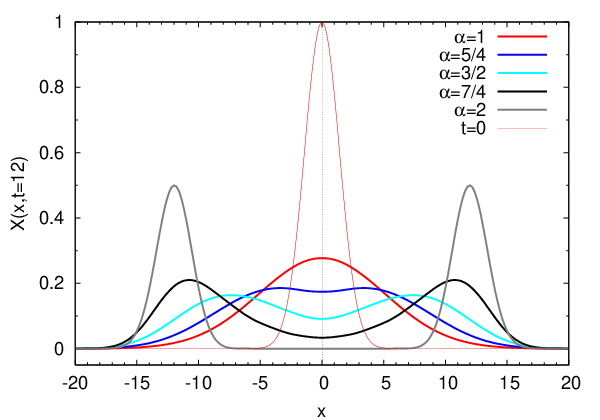
For one spatial dimension $N=n\cdot m<10^{4}$ is usually sufficient for obtaining a reasonable approximate numerical solution. For such $N$ the set of linear equations (12) can be solved by standard methods (e.g. LU decomposition). In fig. 1 we show numerical solutions to (1) for $\alpha=1,\frac{5}{4},\frac{3}{2},\frac{7}{4}$ and 2, at two particular time instants $t=6$ and $t=12$ . The value of $\sigma$ in the initial condition was taken as $\sigma=1$ . The reader can easily see a transition from a diffusion-like solution for $\alpha=1$ , through intermediate cases for $1<\alpha<2$ , to a wave-like solution for $\alpha=2$ .

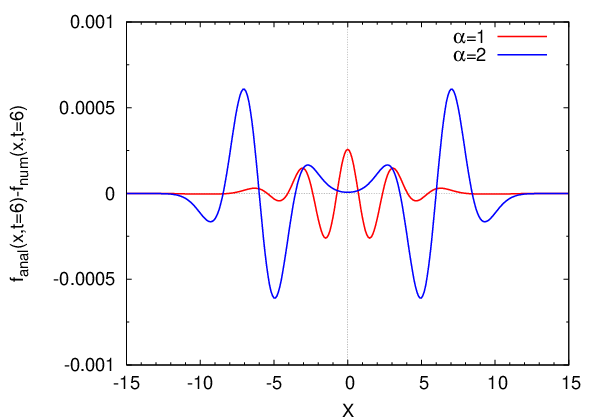
The knowledge of the analytical form of solutions for $\alpha=1$ and 2 allows us to keep approximation errors within a required range. To maintain the errors $\epsilon(x,t)=|f_{\mathrm{anal}}(x,t)-f_{\mathrm{num}}(x,t)|\leq 10^{-3}$ it was enough, for $t=6$ , to take into account a grid of $m=151$ points in $x$ -coordinate, covering the interval $x\in[-15,15]$ and subspace $H_{n}$ with $n=8$ . For $t=12$ case and the same error bounds the grid had to be increased to $m=201$ points for the interval $x\in[-20,20]$ and subspace $H_{n}$ to $n=18$ . Fig. 2 presents approximation errors $\epsilon(x,t)$ for $t=6$ and $\alpha=1$ and 2.

For larger times the number of grid points and size of subspace $H_{n}$ has to grow in order to keep the same precision of numerical solutions. As the matrix $\underline{\mathcal{A}}$ is sparse (among $n^{2}\cdot m^{2}$ elements of $\underline{\mathcal{A}}$ at most $n^{2}(3m-2)$ are non-zero) iterative methods for solving (12) become necessary.

For stochastic equation (2) we need some assumptions for the process $W$ . For the first attempt we assumed that the process $W$ is uniform in time, i.e. $W(x,t)=CW_{1}(x,t)$ (the constant $C$ represents a ’strength’ of the stochastic forces). Then we can approximate the convolution $\int_{0}^{t}S(t-s)dW(s,x)$ in (2) in the following way:

\int_{0}^{t}S(t-s)dW(s,x)=\sum_{i=0}^{I-1}S(t-s_{i})[W(s_{i+1},x)-W(s_{i},x)],

(14)

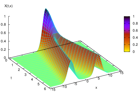
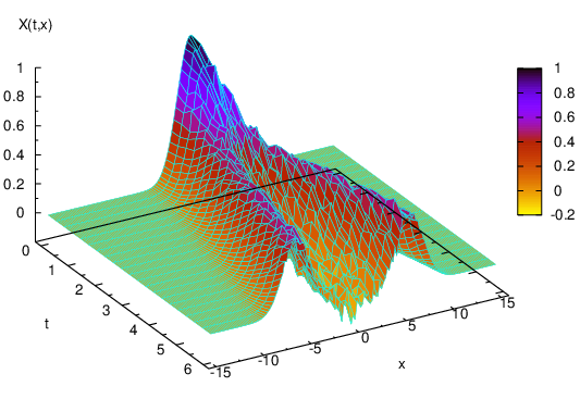
where the time interval $[0,t]$ was divided into a time grid $\{t_{i}=i\tau,~i=0,1,\ldots,I\}$ , $\tau=\frac{t}{I}$ . For cases $\alpha=1$ and 2, when $S(t)$ is known analytically (see (4) and (1)) the stochastic convolution can be computed numerically. Fig. 3 compares the time evolution of solutions obtained numerically for $\alpha=2$ and $t\in[0,6]$ . The top part represents the solution of the deterministic equation (1), the bottom one an example of a single stochastic trajectory (solution of the stochastic equation (2) with $W$ uniform in time, $C=0.1$ ). For more details and examples of numerical results, see [5].

3 Galerkin method, case $d=2$ .

For $d=2$ the equation (12) reads

	$\displaystyle g_{j}(x_{i},y_{l})$	$\displaystyle=$	$\displaystyle c_{j}(x_{i},y_{l})+\frac{1}{h^{2}}\sum_{k=1}^{n}a_{jk}\,[-c_{k}(x_{i-1},y_{l})-c_{k}(x_{i},y_{l-1})$		(16)
			$\displaystyle+4c_{k}(x_{i},y_{l})-c_{k}(x_{i+1},y_{l})-c_{k}(x_{i},y_{l+1})]\;,$		(16)

with $j=1,2,\ldots,n,~i=1,2,\ldots,m,~l=1,2,\ldots,m$ .

Now, in matrix equation

\underline{\mathcal{A}}\,\underline{c}=\underline{g},

(17)

$\underline{c}~$ and $~\underline{g}~$ are $N=n\cdot m^{2}$ -dimensional vectors, such that
$\underline{c}^{T}=c_{1}(x_{1},y_{1}),\ldots,c_{1}(x_{1},y_{m}),c_{1}(x_{2},y_{1})\ldots,c_{1}(x_{2},y_{m}),\ldots,c_{n}(x_{m},y_{m})$ ,
$\underline{g}^{T}=g_{1}(x_{1},y_{1}),\ldots,g_{1}(x_{1},y_{m}),g_{1}(x_{2},y_{1})\ldots,g_{1}(x_{2},y_{m}),\ldots,g_{n}(x_{m},y_{m})$
and

\underline{\mathcal{A}}=\left(\begin{array}[]{ccc}\left[A_{11}\right]&\ldots&\left[A_{1n}\right]\\ \left[A_{21}\right]&\ldots&\left[A_{2n}\right]\\ \vdots&\cdots&\vdots\\ \left[A_{n1}\right]&\ldots&\left[A_{nn}\right]\end{array}\right).

(18)

Now, every block $[A_{ij}]$ is the tridiagonal matrix composed of smaller blocks

[A_{ij}]=\left(\begin{array}[]{ccccccc}(\alpha)_{ij}&(\beta)_{ij}&(0)&(0)&(0)&\cdots&(0)\\ (\beta)_{ij}&(\alpha)_{ij}&(\beta)_{ij}&(0)&(0)&\cdots&(0)\\ (0)&(\beta)_{ij}&(\alpha)_{ij}&(\beta)_{ij}&(0)&\cdots&(0)\\ \vdots&\cdots&&\cdots&&\cdots&\vdots\\ (0)&(0)&\cdots&(0)&(\alpha)_{ij}&(\beta)_{ij}&(0)\\ (0)&(0)&(0)&\cdots&(\beta)_{ij}&(\alpha)_{ij}&(\beta)_{ij}\\ (0)&(0)&(0)&(0)&\cdots&(\beta)_{ij}&(\alpha)_{ij}\end{array}\right).

(19)

Blocks $(\alpha_{ij})$ are tridiagonal

\!\!(\alpha_{ij})\!\!=\!\!\left(\!\!\!\begin{array}[]{ccccccc}\delta_{ij}\!+\!\frac{4}{h^{2}}a_{ij}&\!\!\frac{-1}{h^{2}}a_{ij}&\!\!0&\!\!0&\!\!\ldots&\!\!0&\!\!0\\ \frac{-1}{h^{2}}a_{ij}&\!\!\delta_{ij}\!+\!\frac{4}{h^{2}}a_{ij}&\!\!\frac{-1}{h^{2}}a_{ij}&\!\!0&\!\!\ldots&\!\!0&\!\!0\\ 0&\!\!\frac{-1}{h^{2}}a_{ij}&\!\!\delta_{ij}\!+\!\frac{4}{h^{2}}a_{ij}&\!\frac{-1}{h^{2}}a_{ij}&\!\!\ldots&\!\!0&\!\!0\\ \vdots&\!\!\vdots&\!\!\vdots&\!\!\vdots&\!\!\vdots&\!\!\vdots&\!\!\vdots\\ 0&\!\!0&\!\!0&\!\!\ldots&\!\!\frac{-1}{h^{2}}a_{ij}&\!\delta_{ij}\!+\!\frac{4}{h^{2}}a_{ij}&\!\!\frac{-1}{h^{2}}a_{ij}\\ 0&\!\!0&\!\!0&\!\!0&\!\!\ldots&\!\!\frac{-1}{h^{2}}a_{ij}&\!\!\delta_{ij}\!+\!\frac{4}{h^{2}}a_{ij}\end{array}\!\!\right)\!\!,

(20)

blocks $(\beta_{ij})$ are diagonal

(\beta_{ij})=\left(\begin{array}[]{ccccccc}\frac{-1}{h^{2}}a_{ij}&0&0&0&0&\ldots&0\\ 0&\frac{-1}{h^{2}}a_{ij}&0&0&0&\ldots&0\\ 0&0&\frac{-1}{h^{2}}a_{ij}&0&0&\ldots&0\\ \vdots&\vdots&\vdots&\vdots&\vdots&\vdots&\vdots\\ 0&0&0&\ldots&0&\frac{-1}{h^{2}}a_{ij}&0\\ 0&0&0&0&\ldots&0&\frac{-1}{h^{2}}a_{ij}\end{array}\right)

(21)

and (0) are zeros, each of size $m\cdot m$ .

Dimension of vectors $\underline{c}~\mbox{and}~\underline{g}$ is $N=n\cdot m^{2}$ . Already for $n\!=\!16,~m\!=\!200$ , $N$ becomes large, reaching value of $N=6.4\cdot 10^{5}$ unknowns and the number of matrix elements for the matrix $\underline{\mathcal{A}}$ reaches $~N^{2}=n^{2}m^{4}>4\cdot 10^{11}$ .

Fortunately, the matrix $\underline{\mathcal{A}}$ is sparse. Blocks $[A_{ij}]$ have at most $m(3m-2)+2(m-1)m$ non-zero elements. Then the number of non-zero elements of matrix $\underline{\mathcal{A}}$ is at most (some $a_{ij}$ could be $0$ )

\mathcal{N}\leq n^{2}m(5m-4).

(22)

For $n=16,~m=200$ ,

\mathcal{N}\leq 5.12\cdot 10^{7}

(23)

The size of $\underline{\mathcal{A}}$ and its sparseness property makes using iterative methods for $d\geq 2$ necessary.

3.1 Conjugate and Bi-Conjugate Gradient Method

If matrix $A$ is symmetric and positive definite, then the problem $A\underline{x}=\underline{b}$ is equivalent to minimizing the function $f(\underline{x})=\frac{1}{2}\underline{x}\cdot A\cdot\underline{x}-\underline{b}\cdot\underline{x}$ . This function is minimized when its gradient $\nabla f=A\cdot\underline{x}-\underline{b}$ is zero. In such case a variant of Conjugate Gradient Method is applicable [7, 1, 10].

In our problems the matrix $\underline{\mathcal{A}}$ is not symmetric. Therefore a more complicated Bi-Conjugate Gradient Method is required [7, 1, 10].

3.2 Preconditionig

The convergent rate of iterative methods depends strongly on spectral properties of the matrix $\underline{\mathcal{A}}$ . Usually matrix $\underline{\mathcal{A}}$ is ill-conditiond. The condition number $\kappa=\lambda_{\mathrm{max}}/\lambda_{\mathrm{min}}$ is big ( $\lambda_{i}$ denotes an eigenvalue). Then the convergence of iterations is usually so slow that accumulation of numerical errors often makes obtaining the solution impossible. The remedy is preconditioning. Suppose that $M$ is a matrix that approximates $\underline{\mathcal{A}}$ , but easier to invert. We can solve $\underline{\mathcal{A}}\cdot\underline{x}=\underline{b}$ indirectly by solving $M^{-1}\cdot\underline{\mathcal{A}}\cdot\underline{x}=M^{-1}\cdot\underline{b}$ . If $\kappa(M^{-1}\underline{\mathcal{A}})\ll\kappa(\underline{\mathcal{A}})$ , the number of iterations is reduced significantly.

There are several ways of choosing a preconditioner matrix $M$ . In our case we can take an advantage of knowing detailed structure of matrix $\underline{\mathcal{A}}\,$ (18-(20) which all elements are related to the elements of small matrix $\underline{a}$ (10). Blocks $[A_{ij}]$ (19) and $(\alpha_{ij})$ (20) are tridiagonal. We choose the preconditioner matrix $M$ in the same block form as the matrix $\underline{\mathcal{A}}\,$ , but leaving only diagonal blocks $(\alpha_{ij})$ in (19) and diagonal elements $\delta_{ij}+\frac{1}{h^{2}}a_{ij}$ in (20). All other elements of $(\alpha_{ij})$ and $(\beta_{ij})$ are set equal zero. Then the matrix $M$ has block form with diagonal blocks containing the same element $\gamma_{ij}=\delta_{ij}+\frac{4}{h^{2}}a_{ij}$ on their diagonals. Hence the matrix $M^{-1}$ has the same block structure, with elements $\gamma^{-1}$ on block’s diagonals. The size of $\gamma$ is only $n\cdot n$ , so $\gamma^{-1}$ can be calculated easily by standard methods with the machine precision. The resulting matrix $M^{-1}\underline{\mathcal{A}}\,$ has usually the condition number several orders of magnitude smaller than that of the original matrix $\underline{\mathcal{A}}\,$ . In calculations leading to results presented below such kind of preconditionig allows to obtain a reasonable accuracy within $10^{2}-10^{4}$ iterations for problems with $\sim 10^{5}$ unknowns.

3.3 Numerical results

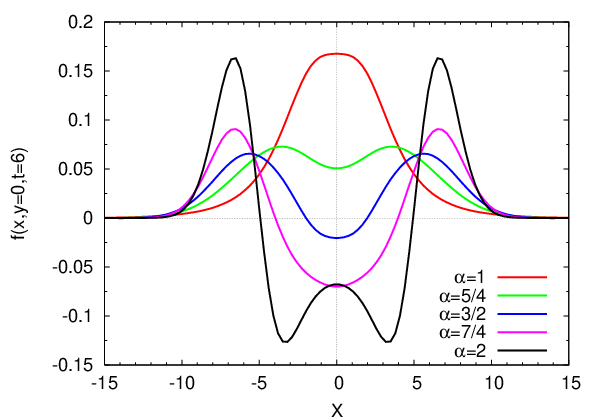
Solutions to deterministic equation (1) for $d=1$ and $d=2$ differ substantially from each other. In fig. 4 we present the numerical solutions to (1) for 2 spatial dimensions in a way convenient for comparison with fig. 1 (top) presenting solutions to (1) for 1 spatial dimension. The initial condition for results displayed in fig. 4 is in the form $f(x,y,0)=\exp[-\frac{x^{2}+y^{2}}{\sigma^{2}}],~\sigma=2$ . The curves in fig. 4 represent cuts of solutions $f(x,y,t)$ along $y=0$ , i.e. $f(x,0,t)$ and it is clearly seen that for all given values of $\alpha$ the profiles of the solutions for $d=1$ and $d=2$ are different.

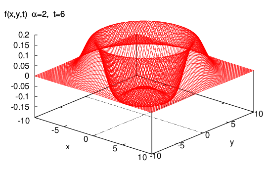
In fig. 5 two examples of the solutions $f(x,y,t)$ at $t=6$ are displayed. In the upper part the case $\alpha=2$ and radially symmetric initial condition is shown. In the lower part the case $\alpha=\frac{7}{4}$ with radially asymmetric initial condition ( $f(x,y,0)=\exp[-\frac{(x+y)^{2}}{\sigma_{1}^{2}}-\frac{(x-y)^{2}}{\sigma_{2}^{2}}]$ , with $\sigma_{1}=4$ , $\sigma_{2}=2$ ) is presented.

References

[1] R. Barrett, M. Berry, T.F. Chan, J. Demmel, J.M. Donato, J. Dongarra, V. Eijkhout, R. Pozo, C. Romine, H. Van der Vorst, Templates for the solution of Linear Systems: Building Blocks for Iterative Methods, Philadelphia, PA: SIAM, (1994).
http://www.netlib.org/linalg/html_templates/Templates.html.
[2] Y. Fujita, Integrodifferential equations which interpolates the heat equation and the wave equation, J. Math. Phys. 30 (1989), 134–144.
[3] M.E. Gurtin and A.C. Pipkin, A general theory of heat conduction with finite wave speeds, Arch. Ration. Mech. Anal. 31 (1968), 40–50.
[4] A. Karczewska, Function–valued stochastic convolutions arising in integrodifferential equations,
preprint http://xxx.lanl.gov/ps/math.PR/0412495.
[5] A. Karczewska and P. Rozmej, On numerical solutions to stochastic Volterra equations, preprint http://xxx.lanl.gov/ps/math.PR/0409026.
[6] R.K. Miller, An integrodifferential equation for rigid heat conductors with memory, J. Math. Anal. Appl. 66 (1978), 313–332.
[7] W.H. Press, S.A. Teukolsky, W.T. Vetterling and B.P. Flannery, Numerical Recipes in Fortran sec.ed., Cambridge University Press, New York, (1992).
[8] J. Prüss, Evolutionary integral equations and applications, Birkhäuser, Basel, 1993.
[9] W. R. Schneider & W. Wyss, Fractional diffusion and wave equations, J. Math. Phys. 30 (1989), 134–144.
[10] J.R. Shewchuk, An Introduction to the Conjugate Gradient Method Without the Agonizing Pain, 1994. School of Computer Science. Carnegie Mellon University.
http://www.cs.cmu.edu/~quake-papers/painless-conjugate-gradient.pdf