Homogeneity of dynamically defined wild knotsThanks: AMS Subject Classification. Primary: 57M30. Secondary: 57M45, 57Q45,30F14. Key Words. Wild knots and Kleinian Groups.

The birth of wild topology was in the 1920’s with works of Alexander, Antoine, Artin and Fox, among others. At that time one of the main problems was to generalize the Schoenflies Theorem. Let $S$ be a simple closed surface in $\mathbb{R}^{3}$ which is homeomorphic to the unit sphere $\mathbb{S}^{2}$. Let $h$ be a homeomorphism of $S$ onto the unit sphere $\mathbb{S}^{2}$ in $\mathbb{R}^{3}$. Is there an extension $\tilde{h}$ of $h$ such that $\tilde{h}$ is a homeomorphism of $\mathbb{R}^{3}$ onto itself? Alexander proved this result in the special case that $S$ is a finite polytope. At the same time, however, he gave his famous example, the Alexander horned sphere, where its unbounded complement in $\mathbb{R}^{3}$ is not simply connected and, in fact, its fundamental group is infinitely generated. Since the complement of $\mathbb{S}^{2}$ in $\mathbb{R}^{3}$ is not simply connected, it follows that no homeomorphism of $\mathbb{R}^{3}$ onto itself will send the horned sphere onto $\mathbb{S}^{2}$ (see [9], [5]). The work of Alexander was published in 1924.

In 1948, Artin and Fox gave the definition of tame embeddings and wild embeddings and constructed a number of surprising examples. For instance, see Figure 1.

Many works by Antoine, Bing, Harold, Moise, Mazur, Brown, Montesinos, among others have contributed much to the understanding of wild sets in $\mathbb{R}^{3}$.

Let $K\subset\mathbb{S}^{3}$ be a knot. We say that a point $x\in K$ is locally flat if there exists an open neighborhood $U$ of $x$ such that there is a homeomorphism of pairs: $(U,U\cap K)\sim(Int(\mathbb{B}^{3}),Int(\mathbb{B}^{1}))$. Otherwise, $x$ is said to be a wild point. A knot $K$ is a wild knot if it contains at least one wild point.

We say that a knot $K\subset\mathbb{S}^{3}$ is homogeneous if given two points $p$, $q\in K$, there exists a homeomorphism $\psi:\mathbb{S}^{3}\rightarrow\mathbb{S}^{3}$ such that $\psi(K)=K$ and $\psi(p)=q$.

The wild knot $K$ given by Artin and Fox (Figure 1) is not homogeneous. In fact, it contains just one wild point $p$, hence it is not possible to give a homeomorphism $\psi:\mathbb{S}^{3}\rightarrow\mathbb{S}^{3}$ such that $\psi(K)=K$ and $\psi(p)=q$, $q\neq{p}$, since any homeomorphism sends wild points into wild points. In general, wild knots are not homogeneous.

The purpose of this paper is to show that dynamically defined wild knots (see section 2) are homogeneous. In section 3, we will give a proof of this fact.

In this section, we will describe the construction of dynamically defined wild knots. We will begin with some basic definitions.

Let $M\ddot{o}b(\mathbb{S}^{n})$ denote the group of Möbius transformations of the n-sphere $\mathbb{S}^{3}=\mathbb{R}^{n}\cup\{\infty\}$ i.e. the group of diffeomorphisms of the n-sphere that preserves angles with respect to the standard metric. Let $\Gamma\subset M\ddot{o}b(\mathbb{S}^{n})$ be a discrete subgroup. Then $x\in\mathbb{S}^{3}$ is a point of discontinuity for $\Gamma$ if there is a neighborhood $U$ of $x$ such that $U\cap gU\neq\emptyset$ only for finitely many $g\in\Gamma$. The domain of discontinuity $\Omega(\Gamma)$ consists of all points of discontinuity.

Next, we will give the construction of dynamically defined wild knots.

If the points of tangency are joined by spherical geodesic segments in $\mathbb{S}^{3}$, we obtain a polygonal knot $K_{1}$. It is called the polygonal template of $T_{1}$. We define the filled-in $T$ as $|T_{1}|=\cup^{n}_{i=1}B_{i}$, where $B_{i}$ is the round closed 3-ball whose boundary $\partial B_{i}$ is $\Sigma_{i}$.

Let $\Gamma$ be the group generated by reflections $I_{j}$, through $\Sigma_{j}$ ($j=1,\ldots,n$). Then $\Gamma$ is a Kleinian group. We will describe geometrically the action of $\Gamma$.

1. 1.

   First stage: Observe that when we reflect with respect to each $\Sigma_{k}$ ($k=1,2,\ldots,n$), a mirror image of $K_{1}$ is mapped into the ball $B_{k}$ (see Figure 3).

   

   After reflecting with respect to each pearl, we obtain a new necklace $T_{2}$ of $n(n-1)$ pearls, subordinate to a new knot $K_{2}$; which is in turn isotopic to the connected sum of $n+1$ copies of $K_{1}$ (see Figure 2).

   

2. 2.

   Second stage: Now, we reflect with respect to each pearl of $T_{2}$. When we are finished, we obtain a new necklace $T_{3}$ of $n(n-1)^{2}$ pearls. Its template is a polygonal knot $K_{3}$; which is in turn isotopic to the connected sum of $n^{2}-n+1$ copies of $K_{1}$ and $n$ copies of its mirror image (recall that composition of an even number of reflections is orientation-preserving). Observe that $|T_{3}|\subset|T_{2}|$ (see Figure 5).

   

3. 3.

   $k^{th}$-Stage: We reflect with respect of each pearl of $T_{k}$. At the end of this stage, we obtain a new necklace $T_{k+1}$ of $n(n-1)^{k}$ pearls, subordinate to a polygonal knot $K_{k+1}$. By construction, $|T_{k+1}|\subset|T_{k}|$.

Then, the limit set is given by the inverse limit (see [6], [8])

It has been proved (see [6], [8]) that the limit set $\Lambda(\Gamma)$ is a wild knot in the sense of Artin and Fox. It is called a dynamically-defined wild knot.

Let $T_{1}$ be a $n_{1}$-pearl necklace subordinate to the polygonal knot $K_{1}$. We can assume without loss of generality that $K_{1}\subset{\mathbb{R}}^{3}\subset{\mathbb{S}}^{3}=\mathbb{R}^{3}\cup\{\infty\}$.

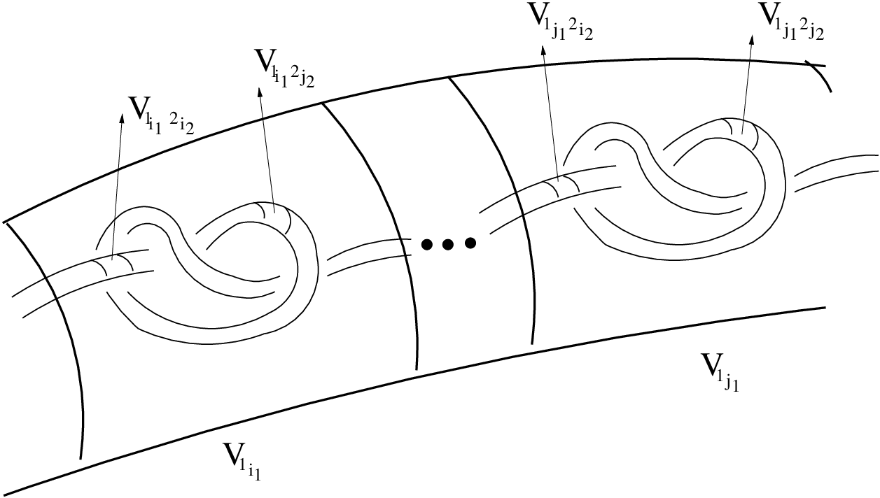
Let $V_{1}$ be a closed tubular neighborhood of $K_{1}$ and $\pi_{1}:V_{1}\to{K_{1}}$ the projection. We can assume that $\pi_{1}^{-1}(\{x\})$ is an euclidean 2-disk of radius $r_{1}>0$ independent of $x$. If $\{p_{1_{1}},\ldots,p_{1_{n_{1}}}\}$ are the points of tangency of consecutive pearls of $T_{1}$, we can also assume that $\pi_{1}^{-1}(\{p_{1_{j}}\})$ is tangent to the consecutive pearls at $p_{1_{j}}\,$ ($1\leq{j}\leq{n_{1}}$). The tubular neighborhood $V_{1}$ is the union of $n_{1}$ “solid cylinders” $V_{1_{1}}\ldots V_{1_{n_{1}}}$ where $V_{1_{j}}=\pi_{1}^{-1}(\{[p_{1_{j}},p_{1_{j+1}}]\})$ is called solid cylinder, since it is homeomorphic to a solid cylinder $C=\mathbb{D}^{2}\times[0,1]$ (see Figure 6).

For the second stage, we have a pearl necklace $T_{2}$ with $n_{2}$ pearls subordinate to the polygonal knot $K_{2}$. Let $V_{2}\subset\mbox{Int}(V_{1})$ be a closed tubular neighborhood of $K_{2}$ and $\pi_{2}:V_{2}\to{K_{2}}$ be the projection. We again assume that $\pi_{2}^{-1}(\{x\})$ is an euclidean 2-disk of radius $r_{2}>0$ independent of $x$. Notice that the points $\{p_{1_{1}},\ldots,p_{1_{n_{1}}}\}$ are also points of tangency of consecutive pearls of $T_{2}$. We will denote by $\{p_{1_{i},2_{1}},\ldots,p_{1_{i},2_{n-1}}\}\subset T_{2}$ the corresponding points of tangency of consecutive pearls of $V_{1_{i}}\cap V_{2}$, $1\leq i\leq n$. We can again assume that $\pi_{2}^{-1}(\{p_{1_{i},2_{j}}\})$ is tangent to the consecutive pearls at $p_{1_{i},2_{j}}\,$ ($1\leq i\leq n$, $1\leq j\leq n-1$). The tubular neighborhood $V_{2}$ is the union of $n_{2}$ solid cylinders $V_{1_{i}2_{j}}$ ($1\leq i\leq n$, $1\leq j\leq n-1$) where $V_{1_{i}2_{j}}=\pi_{2}^{-1}(\{[p_{1_{i}2_{j}},p_{1_{i}2_{j+1}}]\})$.

We continue inductively, so at the end of the $k$-stage of the reflecting process, we have the pearl necklace $T_{k}$ with $n_{k}$ pearls subordinate to the polygonal knot $K_{k}$. Let $V_{k}$ be a closed tubular neighborhood of $K_{k}$ such that $V_{k}\subset\mbox{Int}(V_{k-1})$. Let $\pi_{k}:V_{k}\to{K_{k}}$ be the projection. We assume that $\pi_{k}^{-1}(\{x\})$ is an euclidean 2-disk of radius $r_{k}>0$ independent of $x$. We will denote by $\{p_{1_{i_{1}},2_{i_{2}},\ldots,k_{1}},\ldots,p_{1_{i_{1}},2_{i_{2}},\ldots,k_{n-1}}\}\subset T_{k}$ the corresponding points of tangency of consecutive pearls of $(V_{1_{i_{1}},2_{i_{2}},\ldots,(k-1)_{i_{k-1}}})\cap V_{k}$, $1\leq i_{1}\leq n$ and $1\leq i_{2},\ldots i_{k-1}\leq n-1$. The tubular neighborhood $V_{k}$ is the union of $n_{k}$ solid cylinders $V_{1_{i_{1}},2_{i_{2}},\ldots,(k-1)_{i_{k-1}},k_{i_{k}}}$. Notice that $\lim_{k\rightarrow\infty}r_{k}=0$ and $\Lambda=\cap_{k=1}^{\infty}V_{k}$.

Let $p$, $q\in\Lambda$. There exist two sequences of solid cylinders $\{V_{1_{i_{1}},2_{i_{2}},\ldots,n_{i_{n}}}\}$, and $\{V_{1_{j_{1}},2_{j_{2}},\ldots,n_{j_{n}}}\}$ where $V_{1_{i_{1}},2_{i_{2}},\ldots,n_{i_{n}}}$ and $V_{1_{j_{1}},2_{j_{2}},\ldots,n_{j_{n}}}\in V_{n}$, such that $p=\cap_{n=1}^{\infty}V_{1_{i_{1}},2_{i_{2}},\ldots,n_{i_{n}}}$ and $q=\cap_{n=1}^{\infty}V_{1_{j_{1}},2_{j_{2}},\ldots,n_{j_{n}}}$. In fact, these sequences converge to $p$ and $q$ respectively, with respect to the Hausdorff metric of closed sets on $\mathbb{S}^{3}$.

We define the homeomorphism $F_{0}:(\mathbb{S}^{3}-\mbox{Int}(V_{1}))\rightarrow(\mathbb{S}^{3}-\mbox{Int}(V_{1}))$ such that it sends $\partial V_{1_{i_{1}}}\cap\partial V_{1}$ into $\partial V_{1_{j_{1}}}\cap\partial V_{1}$, $\partial V_{1_{i_{1}+1}}\cap\partial V_{1}$ into $\partial V_{1_{j_{1}+1}}\cap\partial V_{1}$ and so on. This map also sends $\pi_{1}^{-1}(p_{1_{i_{1}}})\cap V_{1}$ into $\pi_{1}^{-1}(p_{1_{j_{1}}})\cap V_{1}$, $\pi_{1}^{-1}(p_{1_{i_{1}+1}})\cap V_{1}$ into $\pi_{1}^{-1}(p_{1_{j_{1}+1}})\cap V_{1}$ and so on.

Next, we will define a homeomorphism $f_{1}:(\partial V_{1}\cup\partial V_{2})\rightarrow(\partial V_{1}\cup\partial V_{2})$ such that $f_{1}|_{\partial V_{1}}=F_{0}$. Let $B_{1_{k_{1}}}=\cup_{k_{2}=1}^{n-1}V_{1_{k_{1}}2_{k_{2}}}$. The pair $(V_{1_{k_{1}}},B_{1_{k_{1}}}\cap V_{2})$ is a solid tangle; i.e. a solid cylinder with a knotted hole (see Figure 7), and it is homeomorphic to the solid tangle $(C,\tilde{K})$, where $C$ is a solid cylinder and $\tilde{K}$ is the mirror image of the knot $K$ via the homeomorphism $h_{1_{k_{1}}}$, which will be used below.

Since, $F_{0}$ sends $\partial V_{1_{k_{1}}}\cap V_{1}$ into $\partial V_{1_{l_{1}}}\cap V_{1}$, we define the map $f_{1}$ in the following way. If $k_{1}\neq i_{1}$, then $f_{1}$ sends the pair $(\partial V_{1_{k_{1}}},\partial B_{1_{k_{1}}}\cap V_{2})$ into $(\partial V_{1_{l_{1}}},\partial B_{1_{l_{1}}}\cap V_{2})$, where $\partial V_{1_{k_{1}}2_{k_{2}}}\cap V_{2}$ is sent to $\partial V_{1_{l_{1}}2_{k_{2}}}\cap V_{2}$ and ($\pi_{1}^{-1}(p_{1_{k_{1}}})-\mbox{Int}(\pi_{2}^{-1}(p_{1_{k_{1}}2_{k_{2}}}))$) is sent to ($\pi_{1}^{-1}(p_{1_{l_{1}}})-\mbox{Int}(\pi_{2}^{-1}(p_{1_{l_{1}}2_{k_{2}}}))$). If $k_{1}=i_{1}$, then $f_{1}$ sends the pair $(\partial V_{1_{i_{1}}},\partial B_{1_{i_{1}}}\cap V_{2})$ into $(\partial V_{1_{j_{1}}},\partial B_{1_{j_{1}}}\cap V_{2})$ such that $\partial V_{1_{i_{1}}2_{i_{2}}}\cap V_{2}$ goes into $\partial V_{1_{j_{1}}2_{j_{2}}}\cap V_{2}$ and ($\pi_{1}^{-1}(p_{1_{i_{1}}})-\mbox{Int}(\pi_{2}^{-1}(p_{1_{i_{1}}2_{i_{2}}}))$) is sent to ($\pi_{1}^{-1}(p_{1_{j_{1}}})-\mbox{Int}(\pi_{2}^{-1}(p_{1_{j_{1}}2_{j_{2}}}))$) (see Figure 8).

Notice that the composition map $h_{1_{l_{1}}}\circ f_{1}\circ h_{1_{k_{1}}}^{-1}$ is isotopic to the identity map $I_{(C,\tilde{K})}$ and this fact will be used to extend the map $f_{1}$ to a map $F_{1}:(V_{1}-\mbox{Int}(V_{2}))\rightarrow(V_{1}-\mbox{Int}(V_{2}))$ via the following Lemma.

Proof. Let $\psi:\partial M\times[0,1]\to M$ be a collaring of the boundary, i.e., $\psi$ is a homeomorphism such that $\psi(x,0)=x$. Let $N=\psi(\partial M\times[0,1])\subset M$. Let $\{g_{t}\},\,\,t\in[0,1],$ be an isotopy of $g$ to the identity, i.e., $g_{o}=g$, $g_{1}=I_{\partial M}$. Let $H:\partial M\times[0,1]\to\partial M\times[0,1]$ be given by the formula $H(x,t)=(g_{t}(x),t)$. Let $G_{0}:N\to N=\psi\circ H\circ\psi^{-1}$. Then we define $G:M\to M$ as $G(y)=G_{0}(y)$ if $y\in N$ and $G(y)=y$ if $y\notin N$. For the rest we simply observe that the fibers of $\pi$ are surfaces that meet transversally the boundary an therefore the collaring can be chosen in such a way that $\psi(\{(x,t)|t\in[0,1]\})$ is contained in a fiber for each fixed $x\in\partial M$. $\blacksquare$

We continue inductively, so at the $k$-stage, we have a homeomorhism $F_{k}:(V_{k}-\mbox{Int}(V_{k+1}))\rightarrow(V_{k}-\mbox{Int}(V_{k+1}))$ such that the solid cylinder $(\partial V_{1_{i_{1}}2_{i_{2}}\ldots k_{i_{k}}},\partial B_{1_{i_{1}}2_{i_{2}}\ldots k_{i_{k}}}\cap V_{k})$ is sent into $(\partial V_{1_{j_{1}}2_{j_{2}}\ldots k_{j_{k}}},\partial B_{1_{j_{1}}2_{j_{2}}\ldots k_{j_{k}}}\cap V_{k})$, in such a way that the cylinder $\partial V_{1_{i_{1}}2_{i_{2}}\ldots(k+1)_{i_{k+1}}}\cap V_{k+1}$ goes into the cylinder $\partial V_{1_{j_{1}}2_{j_{2}}\ldots(k+1)_{j_{k+1}}}\cap V_{k+1}$ and ($\pi_{1}^{-1}(p_{1_{i_{1}}2_{i_{2}}\ldots k_{i_{k}}})-\mbox{Int}(\pi_{2}^{-1}(p_{1_{i_{1}}2_{i_{2}}\ldots(k+1)_{i_{k+1}}}))$) is sent to ($\pi_{1}^{-1}(p_{1_{j_{1}}2_{j_{2}}\ldots k_{j_{k}}})-\mbox{Int}(\pi_{2}^{-1}(p_{1_{j_{1}}2_{j_{2}}\ldots(k+1)_{j_{k+1}}}))$).

This construction allows us to define a map $F:(\mathbb{S}^{3}-\Lambda)\rightarrow(\mathbb{S}^{3}-\Lambda)$ as $F(x)=F_{k}(x)$ if $x\in(V_{k}-\mbox{Int}(V_{k+1}))$. Notice that $F$ is a homeomorphism, since each $F_{k}$ is a homeomorphism and $F_{k}(x)=F_{k+1}(x)$ for $x\in\partial V_{k+1}$ and for all $k$. We extend $F$ to a map $\tilde{F}:\mathbb{S}^{3}\rightarrow\mathbb{S}^{3}$ in the following way. Let $x\in\Lambda$. Then, there exists a sequence of cylinders $\{V_{1_{j_{1}},2_{j_{2}},\ldots,n_{j_{n}}}\}$, where $V_{1_{j_{1}},2_{j_{2}},\ldots,n_{j_{n}}}\subset V_{n}$ such that $x=\cap_{n=1}^{\infty}V_{1_{j_{1}},2_{j_{2}},\ldots,n_{j_{n}}}$. We define $\tilde{F}(x)=\cap{F}(V_{1_{j_{1}},2_{j_{2}},\ldots,n_{j_{n}}})$. Notice that $\tilde{F}$ is well-defined and is continuous. In fact, since $F$ is a homeomorphism, we just need to prove that $\tilde{F}$ is continuous in $\Lambda$. Given $x\in\Lambda$ and let $\{x_{n}\}$ be a sequence that converges to $x$. We can assume, without loss of generality, that $x_{n}\in V_{1_{j_{1}},2_{j_{2}},\ldots,n_{j_{n}}}\subset V_{n}$, hence $\tilde{F}(x_{n})=F(x_{n})\in F(V_{j_{1},j_{2},\ldots,j_{n}})$, so $\lim_{n\rightarrow\infty}F(x_{n})=\tilde{F}(x)$. Therefore, $\tilde{F}$ is continuous.

Proof. Since $\Lambda=\cap_{k=1}^{\infty}V_{k}$, and $\tilde{F}(V_{k})=V_{k}$, we have that $\tilde{F}(\Lambda)=\Lambda$.

Next, we will prove that $\tilde{F}$ is a bijection. Since $\tilde{F}|_{\mathbb{S}^{3}-\Lambda}$ is a bijection, it is enough to prove that $\tilde{F}|_{\Lambda}$ is it. Let $a$, $b\in\Lambda$. Then $a=\cap V_{1_{l_{1}},2_{l_{2}},\ldots,n_{l_{n}}}$ and $b=\cap V_{1_{r_{1}},2_{r_{2}},\ldots,n_{r_{n}}}$, where $V_{1_{l_{1}},2_{l_{2}},\ldots,n_{l_{n}}}$, $V_{1_{r_{1}},2_{r_{2}},\ldots,n_{r_{n}}}\subset V_{n}$. If $\tilde{F}(a)=\tilde{F}(b)$, this implies that $\tilde{F}(V_{1_{l_{1}},2_{l_{2}},\ldots,n_{l_{n}}})\cap\tilde{F}(V_{1_{r_{1}},2_{r_{2}},\ldots,n_{r_{n}}})\neq\emptyset$. Since, $\tilde{F}|_{\mathbb{S}^{3}-\Lambda}$ is a homeomorphism, we have that $V_{1_{l_{1}},2_{l_{2}},\ldots,n_{l_{n}}}\cap V_{1_{r_{1}},2_{r_{2}},\ldots,n_{r_{n}}}\neq\emptyset$, but this is a contradiction. Hence $a=b$. For each $x=\cap V_{1_{j_{1}},2_{j_{2}},\ldots,n_{j_{n}}}\in\Lambda$, let $x^{\prime}=\cap\tilde{F}^{-1}(V_{1_{j_{1}},2_{j_{2}},\ldots,n_{j_{n}}})$. By the above, $\tilde{F}(x^{\prime})=x$. It follows that, $\tilde{F}|_{\Lambda}:\Lambda\rightarrow\Lambda$ is a bijection, hence $\tilde{F}$ is a bijection. Therefore $\tilde{F}:\mathbb{S}^{3}\rightarrow\mathbb{S}^{3}$ is a continuous bijection, hence $\tilde{F}$ is a homeomorphism. $\blacksquare$

Proof. Let $p$, $q\in\Lambda$. Then $p=\cap V_{1_{l_{1}},2_{l_{2}},\ldots,n_{l_{n}}}$ and $q=\cap V_{1_{r_{1}},2_{r_{2}},\ldots,n_{r_{n}}}$, where $V_{1_{l_{1}},2_{l_{2}},\ldots,n_{l_{n}}}$, $V_{1_{r_{1}},2_{r_{2}},\ldots,n_{r_{n}}}\in V_{n}$. By the above, we can construct a homeomorphism $\tilde{F}:\mathbb{S}^{3}\rightarrow\mathbb{S}^{3}$ such that $\tilde{F}|_{\Lambda}=\Lambda$ and $\tilde{F}(p)=\tilde{F}(q)$. Therefore, $\Lambda$ is homogeneous. $\blacksquare$

We recall that a knot or link $L$ in $\mathbb{S}^{3}$ is fibered if there exists a locally trivial fibration $f:(\mathbb{S}^{3}-L)\rightarrow\mathbb{S}^{1}$. We require that $f$ be well-behaved near $L$, that is, each component $L_{i}$ is to have a neighbourhood framed as $\mathbb{D}^{2}\times\mathbb{S}^{1}$, with $L_{i}\cong\{0\}\times\mathbb{S}^{1}$, in such a way that the restriction of $f$ to $(\mathbb{D}^{2}-\{0\})\times\mathbb{S}^{1}$ is the map into $\mathbb{S}^{1}$ given by $(x,y)\rightarrow\frac{y}{|y|}$. It follows that each $f^{-1}(x)\cup L$, $x\in\mathbb{S}^{1}$, is a 2-manifold with boundary $L$: in fact a Seifert surface for $L$ (see [9], page 323).

For dynamically-defined wild knots we have the following result.

Next, we will briefly describe the fiber $\Sigma_{\theta}$. For a proof of the above theorem, see [4].

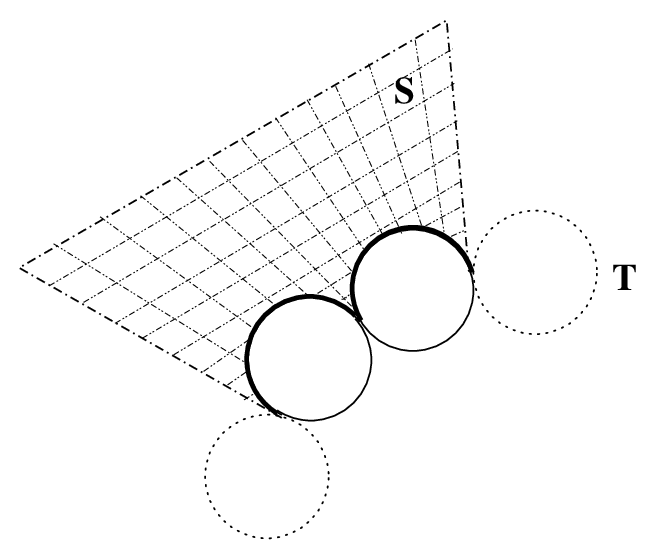
Let $T_{1}$ be a pearl-necklace subordinate to the fibered tame knot $K_{1}$ with fiber $S_{1}$. Let $\widetilde{P}:(\mathbb{S}^{3}-K_{1})\rightarrow\mathbb{S}^{1}$ be the given fibration. Observe that $\widetilde{P}\mid_{\mathbb{S}^{3}-|T_{1}|}\equiv P$ is a fibration and, after modifying $\widetilde{P}$ by isotopy if necessary, we can consider that the fiber $S$ cuts each pearl $\Sigma_{i}\in T_{1}$ in arcs $a_{i}$, whose end-points are $\Sigma_{i-1}\cap\Sigma_{i}$ and $\Sigma_{i}\cap\Sigma_{i+1}$. These two points belong to the limit set (see Figure 9).

The fiber $\widetilde{P}^{-1}(\theta)=P^{-1}(\theta)$ is a Seifert surface $S_{1}^{*}$ of $K_{1}$, for each $\theta\in\mathbb{S}^{1}$. We suppose $S_{1}^{*}$ is oriented.

The reflection $I_{j}$ maps both a copy of $T_{1}-\Sigma_{j}$ (called $T_{1}^{j}$) and a copy of $S_{1}^{*}$ (called $S_{2}^{*j}$) into the ball $B_{j}$, for $j=1,2,\ldots,n$. Observe that both $T_{1}^{j}$ and $S_{2}^{*j}$ have opposite orientation and that $S_{1}^{*}$ and $S_{2}^{*j}$ are joined by the arc $a_{j}$ (see Figure 10) which, in both surfaces, has the same orientation.

The necklaces $T_{1}^{j}$ and $T_{1}$ are joined by the points of tangency of the pearl $\Sigma_{j}$ and the orientation of these two points is preserved by the reflection $I_{j}$. Thus, we have obtained a new pearl-necklace isotopic to the connected sum $T_{1}\#T_{1}^{j}$, whose complement also fibers over the circle with fiber the sum of $S_{1}^{*}$ with $S_{2}^{*j}$ along arc $a_{j}$, namely the fiber is $S_{1}^{*}\#_{a_{j}}S_{2}^{*j}$.

Now do this for each $j=1,\ldots,n$. At the end of the first stage, we have a new pearl-necklace $T_{2}$ whose template is the knot $K_{2}$ (see section 2). Its complement fibers over the circle with fiber the Seifert surface $S^{*}_{2}$, which is in turn homeomorphic to the sum of $n+1$ copies of $S_{1}^{*}$ along the respective arcs.

Continuing this process, we have from the second step onwards, that $n-1$ copies of $S_{1}^{*}$ are added along arcs to each surface $S^{*i}_{k}$, (the surface corresponding to the $k^{th}$ stage). Notice that in each step, the points of tangency are removed since they belong to the limit set, and the length of the arcs $a_{j}$ tends to zero.

From the remarks above, we have that $\Sigma_{\theta}$ is homeomorphic to an orientable infinite-genus surface. In fact, it is the sum along arcs of an infinite number of copies of $S^{*}$.

Using the second part of lemma 3.1 one has the following:

Proof. Let $P:(\mathbb{S}^{3}-K)\rightarrow\mathbb{S}^{1}$ be the given fibration. We can assume that the fiber cuts each pearl $\Sigma_{i}$ of the pearl-necklace as in Figure 9. Let $p$, $q\in\Lambda$. Then, there exist two sequences of solid cylinders $\{V_{1_{i_{1}},2_{i_{2}},\ldots,n_{i_{n}}}\}$, and $\{V_{1_{j_{1}},2_{j_{2}},\ldots,n_{j_{n}}}\}$ where $V_{1_{i_{1}},2_{i_{2}},\ldots,n_{i_{n}}}$ and $V_{1_{j_{1}},2_{j_{2}},\ldots,n_{j_{n}}}\in V_{n}$, such that $p=\cap_{n=1}^{\infty}V_{1_{i_{1}},2_{i_{2}},\ldots,n_{i_{n}}}$ and $q=\cap_{n=1}^{\infty}V_{1_{j_{1}},2_{j_{2}},\ldots,n_{j_{n}}}$. Let $V_{k}$ be as in section 3. Consider the map $f_{k}:(\partial V_{k}\cap\partial V_{k+1})\rightarrow(\partial V_{k}\cap\partial V_{k+1})$.

By the previous description, we know that $V_{1}-\mbox{Int}(V_{2})$ fibers over the circle and that $f_{1}$ leaves invariant the fibers on the boundary. Then by Lemma 3.1, $f_{1}$ admits and extension $F_{1}:(V_{1}-\mbox{Int}(V_{2}))\rightarrow(V_{1}-\mbox{Int}(V_{2}))$ which preserves the fibers. We continue inductively, so at the end of the $k$-stage, we have that the homeomorphism $f_{k}$ preserves the fibers, hence it can be extended to a map $F_{k}:(V_{k}-\mbox{Int}(V_{k+1}))\rightarrow(V_{k}-\mbox{Int}(V_{k+1}))$ which also preserves the fibers.

Let $\tilde{F}:\mathbb{S}^{3}\rightarrow\mathbb{S}^{3}$ be as in section 3. Then, by Theorem 3.2 we have that $\tilde{F}|_{\Lambda}=\Lambda$, $\tilde{F}(p)=\tilde{F}(q)$. The map $F=\tilde{F}|_{\mathbb{S}^{3}-\Lambda}$ defined by $F(x)=F_{k}(x)$ if $x\in(V_{k}-\mbox{Int}(V_{k+1}))$ is a homeomorphism (see section 3) which preserves fibers. Therefore, the result follows. $\blacksquare$

References

• [1] E. Artin, Zur Isotopie zweidimensionalen Flächen im R4R_{4} Abh. Math. Sem. Univ. Hamburg (1926), 174-177.
• [2] R. H. Fox. A Quick Trip Through Knot Theory. Topology of 3-Manifolds and Related Topics. Prentice-Hall, Inc., 1962.
• [3] M. Gromov, H. B. Lawson, W. Thurston. Hyperbolic 4-manifolds and conformally flat 3-manifolds. Publ. Math. I.H.E.S. Vol. 68 (1988), 27-45.
• [4] G. Hinojosa. Wild knots as limit sets of Kleinian Groups. To appear in Contemporary Mathematics.
• [5] J. Hocking, G. Young. Topology. Dover, 1961.
• [6] M. Kapovich. Topological Aspects of Kleinian Groups in Several Dimensions. Preprint (1988).
• [7] M. Kapovich. Hyperbolic Manifolds and Discrete Groups. Progress in Mathematics, Birkhauser, 2001.
• [8] B. Maskit. Kleinian Groups. Springer Verlag, 1987.
• [9] D. Rolfsen. Knots and Links. Publish or Perish, Inc. 1976.
• [10] B. Rushing. Topological Embeddings. Academic Press, 1973, Vol 52.
G. Hinojosa. Universidad Autóma del Estado de Morelos. Av. Universidad 1001, Col. Chamilpa. Cuernavaca, Morelos, México, 62210.
E-mail address:gabriela@servm.fc.uae.mx
A. Verjovsky. Instituto de Matemáticas, Universidad Nacional Autónoma de México, Unidad Cuernavaca. Av. Universidad s/n, Col. Lomas de Chamilpa. Cuernavaca, Morelos México, 62210.
E-mail address: alberto@matcuer.unam.mx