Khovanov-Rozansky homology
of two-bridge knots and linksThanks: The author was supported by an NSF Postdoctoral fellowship.
Abstract.
We compute the reduced version of Khovanov and Rozansky’s homology for two-bridge knots and links. The answer is expressed in terms of the HOMFLY polynomial and signature.
2000 Mathematics Subject Classification
57M271. Introduction
In [10], Khovanov and Rozansky introduced a family of link invariants generalizing the Jones polynomial homology of [8]. In this paper, we will mostly be interested in the reduced version of their homologies, which are invariants of an oriented link together with a marked component of . These invariants take the form of bigraded homology groups , where is a positive integer. The information contained in these groups is conveniently represented by the Poincaré polynomial
| (1) |
Substituting gives the graded Euler characteristic, which is equal to a classical polynomial invariant of — the knot polynomial:
| (2) |
Here is the HOMFLY polynomial of , normalized so that of the unknot is equal to and satisfies the skein relation
| (3) |
For , the Khovanov-Rozansky homology is the same for all links : . When , the theory reduces to the ordinary Khovanov homology, for which extensive computer calculations have been made by Bar-Natan [1], Bar-Natan and Green [2], and Shumakovitch [16]. In contrast, very few computations of the Khovanov-Rozansky homology have been made when . Our aim here is to describe the most elementary type of behavior exhibited by these theories, and to show that it is satisfied by a simple class of links — the two-bridge links. The result is most easily stated for knots:
Theorem 1.
If is a two-bridge knot, then for each , is determined by the HOMFLY polynomial and signature of . In terms of the Poincaré polynomial, the relation may be expressed as follows:
| (4) |
If satisfies the equation above, we say that is -thin (cf. Definition 5.1 of [5].) Thus the theorem may be summarized by saying that two-bridge knots are -thin for all The condition that a knot be -thin generalizes the definition of thinness for the ordinary Khovanov homology given in [9]. Many knots are known to be thin in this sense. In particular, E.S. Lee proved in [12] that any nonsplit alternating link is thin. Unfortunately, this fact does not seem to generalize to the case; in section 5, we give an example of an alternating knot which is not -thin for any . On the other hand, the condition that is largely technical. We expect that two-bridge knots should actually be -thin for all . For , this follows from Lee’s theorem, so only the cases remain unresolved.
This work in this paper was motivated by the desire to provide some computational support for the conjectures about the structure of made in [5]. In this regard, we have been only partly successful, since the knots considered here exhibit only the simplest possible behavior of the Khovanov-Rozansky homology. Still, it is worth noting that for the knots studied in this paper, satisfies both the stabilization and symmetry properties conjectured in [5]. In addition, we have checked that those knots of crossings or fewer admit plausible candidates for the differentials and described there.
Although the details of the proof of Theorem 1 are somewhat messy, the argument itself is quite soft. The main ingredients are the fact that is a link invariant (plus a tiny bit borrowed from the actual proof of invariance in [10]), the skein exact sequence, and the known behavior of for the unknot and unlink. In particular, if the homology groups recently introduced by Khovanov and Rozansky in [11] could be shown to satisfy a skein exact sequence for arbitrary diagrams (rather than just braid diagrams), we expect that an analogous theorem would hold there as well.
The organization of the paper is as follows. The first two sections contain background material on singular knots and the Khovanov-Rozansky homology. In section 4 we give a more general definition of what it means for a knot or link to be -thin and describe some criteria which can be used to prove that a link is thin. Finally, in section 5 we use these criteria to prove the theorem. We conclude by discussing some other knots to which the methods used in the proof can be applied, and by giving a few calculations of the unreduced Khovanov-Rozansky homology.
Acknowledgements. The author would like to thank Nathan Dunfield, Bojan Gornik, Sergei Gukov, Mikhail Khovanov, Ciprian Manolescu, Peter Ozsváth and Zoltán Szabó for many helpful discussions on this subject, and the referee for valuable comments on the manuscript.
2. Invariants of Singular Links
We begin by fixing our notation for link diagrams and their resolutions. Suppose is an oriented link in represented by some planar diagram. Each crossing of the diagram is either positive, like the crossing labeled in Figure 1, or negative, like . (Warning: this sign convention is the opposite of the one used in [10].) We can construct a new oriented link from either by replacing the crossing with its oriented resolution or by switching the sign of the crossing. If we are willing to forget the orientations, we can also form the unoriented resolution .
2.1. Singular links
The original definition of the Khovanov homology involved replacing each crossing of with its oriented and unoriented resolutions. To define their more general homology theory, Khovanov and Rozansky replaced with a third sort of resolution, in which some crossings in the diagram are replaced by the singular diagram of Figure 1. In what follows, we will find it convenient to consider the class of links which contain one such singular crossing.
Definition 2.1.
A singular link is represented by a planar diagram containing precisely one singular crossing. Two such diagrams represent the same link if they are related by a sequence of Reidemeister of moves which take place away from the singular point.

In what follows, links represented by diagrams without any singular crossings will be described as regular, and the generic term link will be used to refer to both regular and singular links. If is a link for which we have a specific diagram and crossing in mind, we will use and to indicate the link in which the crossing has been replaced by the corresponding crossing or resolution in Figure 1. (If we have a singular link, the crossing to be modified will almost always be the singular one.)
Many notions from classical knot theory extend naturally to singular links. We begin with some terminology. If is a regular link, we let denote the number of components in . If we modify a crossing of , we clearly have . Now suppose is singular. The geometric number of components of is defined to be , and the set of components of is equal to the set of components of the resolution for which the maximum is attained.
It is also convenient to consider an invariant which reflects the algebraic number of components of . is a valued invariant which determines things like the parity of the signature and the exponents of the HOMFLY polynomial. If is a regular link, it is defined by . For singular links, is defined to be equal to .
Finally, if is a singular link with components and , we define the linking number of by
| (5) |
where denotes the number of positive/negative crossings in in which one strand belongs to and the other to . Note that need not be an integer: if is a singular link, then .
2.2. The HOMFLY polynomial
We define the HOMFLY polynomial of a singular link by
| (6) | ||||
| (7) |
(The second equality follows from the skein relation.) Since the link types of , and are invariant under moves that take place away from the singular point, the HOMFLY polynomial is clearly an invariant of singular links.
If is a knot, it is not difficult to see that is a Laurent polynomial in and . In general, however, is only a rational function with denominator . Most of the links we will consider have two components. In this case the fractional part is controlled by the following
Lemma 2.2.
Suppose is a two-component link with knots and as its components. Then for any
| (8) |
is a Laurent polynomial in and .
Formulas of this type are well known in the literature, although we have chosen a somewhat nonstandard normalization for the numerator of the fractional part.
Proof.
If , then is divisible by . Thus if the lemma holds for one value of , it holds for all. Suppose for the moment that is a regular link, so that . If is the disjoint union of knots and , then
| (9) | ||||
| (10) |
so the claim holds in this case. Now suppose that and are two diagrams related by a crossing change and that the two strands in the crossing belong to different components. Then the resolved diagram represents a knot , and is a Laurent polynomial. Using the skein relation, it is easy to see that if one of or satisfies the statement of the lemma, then the other does as well. Since the components of any link can be unlinked by a sequence of such crossing changes, the claim holds in the case when is a regular link.
Now suppose that is singular, so that one of , is a knot and the other is a regular two-component link. Suppose is the link. Then is a Laurent polynomial, so by equation (6), the fractional part of is the fractional part of multiplied by . Clearly and , so the lemma holds. On the other hand, if is the link, the fractional part of is the fractional part of multiplied by . Since and , the claim also holds in this case. ∎
2.3. Determinant and signature
The complex determinant of a link is defined by
| (11) |
where is the Jones polynomial of . If , we can decompose it into a product of the usual determinant of and a phase :
| (12) | ||||
| (13) |
When it is defined, amounts to a refinement of the invariant , in the sense that .
Lemma 2.3.
If is a singular link, then .
Proof.
By equation (6),
| (14) |
On the other hand, Kauffman’s unoriented skein relation for the Jones polynomial tells us that
| (15) |
where denotes the writhe of the diagram . Using the relation , this becomes
| (16) |
for some . Substituting gives , and the claim is proved. ∎
If is a regular link, it is well known that the phase can be used to give an inductive characterization of the signature [4]. More precisely, we have
Lemma 2.4.
Suppose is a regular link with nonzero determinant. Then
Lemma 2.5.
Let be a regular link, and let be obtained from by resolving a crossing. If both and have nonzero determinants, then , while if one of the two determinants is nonzero and the other is zero, then
We use this characterization to extend the definition of the signature to singular links with nonzero determinant.
Definition 2.6.
Let be a singular link with nonzero determinant. Then is determined by the requirements that and .
Corollary 2.7.
If , then .
3. Properties of
In this section, we briefly review the construction of the Khovanov-Rozansky groups and describe some of their elementary properties. Our emphasis is on the formal aspects of the theory — in particular, we have suppressed any discussion of matrix factorizations.
3.1. Foams and functors

The category of -manifolds and cobordisms between them plays a foundational role in the construction of the Khovanov homology. To define their more general theory, Khovanov and Rozansky embedded this category in a larger one, which we refer to as the category of planar foams. The objects of this category are oriented four-valent planar graphs whose vertices resemble the singular crossing of Figure 1. We allow the possibility that some components of the graph are pure circles — that is, a single oriented edge with no vertex. This formulation is slightly different from that used [10], where the graphs are trivalent and have two kinds of edges. The two are related by the operation of inserting a thick edge at each four-valent vertex, as illustrated in Figure 2.
Morphisms in the category of cobordisms are generated by certain elementary morphisms (Reidemeister and Morse moves) modulo some relations (the movie moves of [3].) A similar situation applies to the category of foams. Rather than describe all the generators and relations here, we focus on those which are relevant for the definition of . For this purpose, it suffices to consider morphisms which are formal compositions of the elementary morphisms shown in Figure 3, in which we replace a region of the graph isomorphic to the region inside one of the dotted circles with the region inside the other circle. The only relation we will use is the fact that morphisms are far-commutative: if and are morphisms which take place in disjoint circles, then .

For each integer , Khovanov and Rozansky construct a functor from the category of planar foams to the category of vector spaces over . These functors play a role analogous to that of the dimensional TQFT which appears in the definition of the usual Khovanov homology. They are defined using the theory of matrix factorizations, but we will not discuss the details of the construction here. Instead we simply summarize some relevant facts about collected from [10].
is a functor between graded categories. In practical terms, this means that is a -graded vector space, and if is an elementary morphism of the type shown in Figure 3, then is a graded map of degree one. Another important property of is the presence of “edge operators” associated to the edges of a foam . More precisely, we have
Proposition 3.1.
Suppose is a foam, and let be an edge of . Then there is a linear operator which satisfies the following properties:
- (1)
is a graded map of degree .
- (2)
.
- (3)
for any two edges and .
- (4)
is a free module over the ring .
- (5)
The action of commutes with morphisms. In other words, if is a morphism and is a thin edge of , then there is a corresponding edge of , and
- (6)
Let , and be the four edges adjacent to a vertex of , as illustrated in the right-hand side of Figure 3. Then
- (7)
We will also need to know the precise structure of for some simple foams.
Lemma 3.2.
If is the foam consisting of a single circle with edge , then we have , and the grading of is . If is the foam shown in Figure 2, then , where
| (17) |
The grading of is .
3.2. The Khovanov chain complex
Suppose we are given a planar diagram representing an oriented link , and let be the number of nonsingular crossings in . The cube of resolutions of is an -dimensional cube whose vertices are decorated with planar foams and whose edges are decorated with morphisms between them. More precisely, each nonsingular crossing of may be resolved in the two ways illustrated in Figure 4.

If we resolve every crossing of in one of these ways, the result is clearly a planar foam. Fix once and for all an ordering of the crossings of . Then given a vertex of the cube , we associate to it the foam obtained by resolving the th crossing of in accordance with the th coordinate of .
Let be an edge of the cube with endpoints and , where has one more in its coordinates than . We orient so that it points from to , and write to indicate this fact. The foams and differ only in a neighborhood of a single crossing, where they resemble the two regions of Figure 3. Thus there is an elementary morphism .
By applying the functor , we obtain a cube whose vertices are decorated with graded vector spaces and whose edges are decorated with linear maps between them. We construct a bigraded chain complex from this cube using the method of [8]. As a group, . For , the differential is given by
| (18) |
where the signs are chosen so that every two-dimensional face of the cube has an odd number of minus signs. (This ensures that .) There are many ways to do this, but they all result in isomorphic chain complexes.
The bigrading on is defined as follows. Let be a homogenous element of with grading . Then
| (19) | ||||
| (20) |
where denotes the sum of the coordinates of and and are the number of positive and negative crossings in . The gradings are chosen so that and .
Khovanov and Rozansky showed that the graded Euler characteristic of is the unnormalized polynomial of the link it represents. In other words,
| (21) |
(To be strict, the result of [10] is fomulated for ordinary links. Our definition of the HOMFLY polynomial of a singular link was chosen so that the formula holds in this case as well.)
In contrast to the case of the ordinary Khovanov homology, where the fact that the graded Euler characteristic gives the Jones polynomial is almost immediate from the construction, the proof of this theorem is far from trivial. The argument uses a familiar state model for the polynomial [13] (see also [7] [17]) but also requires a careful analysis of the properties of the functor .
The second major result of [10] is that the homology of the chain complex depends only on , and not on the particular planar diagram that we used to represent it. This group is the unreduced Khovanov-Rozansky homology of , and is denoted by . The theorem is proved by checking that the homology is invariant under the Reidemeister moves, so it applies equally well to both regular and singular links.
3.3. Skein Exact Sequences
Let be a planar diagram of a regular link , and let be a crossing of . Then it is easy to see that there is a short exact sequence
where is the planar diagram in which has been given the resolution, and is the diagram in which has been given the -resolution. We call the resulting long exact sequence on homology a skein exact sequence. These sequences are the main computational tool used in the proof of Theorem 1. For future reference, we record the degrees of the maps involved in them.
Lemma 3.3.
There are long exact sequences
and
3.4. Reduced homology
Let be an edge of the planar diagram , and let be a complete resolution of . Then determines an edge of , and we give the group the structure of a module over by defining for . If is an edge of the cube of resolutions, part (5) of Proposition 3.1 implies that . Thus commutes with the action of , and the chain complex is a module over .
The reduced homology discussed in the introduction is defined to be the homology of the chain complex
| (23) |
where is any edge of belonging to . The homology is independent of the choice of , since any diagram of with a marked point on can be transformed into any other by a sequence of Reidemeister moves and isotopies in which take place away from the marked point.
Applying the decomposition of the previous section to the reduced chain complex, we see that the reduced homology satisfies skein exact sequences analogous to those of Lemma 3.3. Note that these sequences depend not only on the choice of diagram , but also on the choice of the edge in with respect to which we reduce. Varying will result in exact sequences involving the reduced homology with respect to different components.
The module structure of makes into a module over .
Lemma 3.4.
Suppose and belong to the same component of . Then their action on is the same.
Proof.
It suffices to prove the result when and are two edges separated by a single crossing. We assume that the edges near the crossing are labeled as in the right-hand side of Figure 3.
Let be a closed element of , and write for and , where and are the diagrams obtained by giving the and resolution to the crossing in question. Then we can write
| (24) |
where is the differential in and . Since is closed, it follows that and .
The action of the map may be described as follows. Suppose is a vertex of the cube of resolutions of . Then there is a corresponding vertex in the cube of resolutions of , and a unique edge . If , then
| (25) |
Let be the same edge with the opposite orientation, and consider the map given by
| (26) |
Then
| (27) |
by property (7) of Proposition 3.1. Similarly, we find that for .
Consider as an element of . We compute
| (28) | ||||
| (29) | ||||
| (30) | ||||
| (31) | ||||
| (32) |
Thus is homologous to . If the pair of edges in question was and , the claim is proved. On the other hand, if the pair of edges was and , we apply property (6) of Proposition 3.1 to get We then argue as before. ∎
It follows that can be naturally viewed as a module over , where runs over the set of components of . The proof of the lemma carries over verbatim to the reduced complex , so a similar result holds for the reduced homology. In this case, however, the action of the edge is tautologically , so we have
Corollary 3.5.
acts by on whenever belongs to .
4. Thin Knots and Links
In this section, we define what it means for a knot or a two-component link (regular or singular) to be thin, and describe the basic properties of such links. We then give some criteria which can be used to recognize thin links.
4.1. Thin knots
We have already given one formulation of what it means for a knot to be -thin in the introduction. The definition we give here is less compact but perhaps more illuminating.
Definition 4.1.
Let be a Laurent polynomial in and . We say that is alternating if each nonzero term in the sum has the same phase.
Suppose that is a knot and that is its HOMFLY polynomial. Then unless and are both even, so the condition that be alternating amounts to saying that the sign of is determined by the parity of . Starting from , we form the three-variable polynomial
| (33) |
The coefficients of are all positive, so it is potentially a Poincaré polynomial. It is not difficult to see that if we substitute in , we recover if and only if is alternating.
Definition 4.2.
For , a knot is -thin if is alternating and
| (34) |
Corollary 4.3.
If is -thin, then .
Proof.
is alternating, so
| (35) |
since all terms in the first sum have the same phase. ∎
Remark: If is thin, then up to a change of variables (due to differing choices of normalization for ) is the superpolynomial described in [5].
Of course, we should check that the definition given above agrees with the one used in the introduction.
Lemma 4.4.
For , is -thin if and only if
| (36) |
Proof.
Let . If is alternating, then
since the sign of is given by , and by Lemma 2.4 this is also equal to . If is -thin, then is alternating by definition, and substituting = gives the desired result. Conversely, suppose equation (36) holds. Then a term in gives rise to a term
| (37) |
in . For , different values of and always give rise to different exponents of and in , so the sign of each individual term must be positive. Thus , which implies that is alternating and ∎
When , the two formulations diverge. We leave it to the reader to check that in this case, equation (36) is satisfied if and only if the usual Khovanov homology is thin in the sense of [9] and the invariant described in [15] is equal to . In contrast, Definition 4.2 imposes the additional constraint that the HOMFLY polynomial of be alternating. An example of a knot satisfying the first two conditions but not the third is given in section 5.2.
Another useful characterization of thinness is in terms of the -grading defined in [5]. If is a monomial in , we assign to it the -grading . Then equation (33) may be described by saying that if is thin, all terms in have . The corresponding grading on is defined by for . Although is well-defined as an integer, it is best viewed as an element of . Indeed, substituting turns the monomial , which has -grading ) into , which has -grading , and the two quantities agree modulo . Thus if is -thin, for all .
4.2. Thin links
For a number of reasons, the definition of thinness for links is more complicated than for knots. First, there is the question of the module structure. Recall from section 3.4 that is a module over , where runs over the set of components of . The variable corresponding to acts by , so in the case of a knot this issue does not arise. To describe the homology associated to a thin two-component link, however, we must specify not only its Poincaré polynomial, but also its structure as a module, where is the variable corresponding to the unmarked component of .
Second, if is a link with more than one component, is not a Laurent polynomial, and Definition 4.2 cannot be applied. To simplify matters, we assume that is a two-component link (so its HOMFLY polynomial is controlled by Lemma 2.2) and that both components of are unknots. If we further suppose that , we can apply Lemma 2.2 and Corollary 2.7 to write , where
| (38) |
and is a Laurent polynomial in and . Write . In analogy with equation (33), we set
| (39) |
Definition 4.5.
Let be a two-component link both of whose components are unknots and with . If is a component of , we say that the pair is -thin if
- (1)
, where the action of on is trivial.
- (2)
is alternating and the Poincaré polynomial of satisfies
- (3)
The Poincaré polynomial of the second summand is given by
Corollary 4.6.
If is -thin, then .
Proof.
If we substitute and in (38), the second term reduces to , which has the same phase as . It follows that
| (40) |
The second summand clearly has dimension , so the claim follows. ∎
If is -thin, then every element in the first summand has -grading , just as it is for knots. The -grading of the generators of the second summand varies, but it is easy to see that the terms with the highest and lowest -gradings also have -grading congruent to .
4.3. Exact sequences
We are now in a position to state our main technical result.
Theorem 4.7.
Suppose , , and are a knot, a regular two-component link, and a singular two-component link (not necessarily in that order) related by a skein exact sequence, and that
| (41) |
If and are -thin for some , then is -thin as well.
In the interest of maintaining a uniform notation for knots and links, we have omitted mention of the marked components. For those components which are links, the statement should be taken to refer to the reduced homology with respect to the component used to define the skein exact sequence.
Proof.
Without loss of generality, we assume that the sequence is arranged as follows:
For , we define by
| (42) | ||||
| (43) |
Lemma 4.8.
Under the hypotheses of the theorem, is preserved by and , while raises by .
Proof.
The effect of the maps on the -grading is easily determined from Lemma 3.3. It is given by
where the number over each arrow indicates the degree by which it raises . To determine the relation between the signatures, we use the relations
| (44) | ||||
| (45) |
obtained by substituting , in equations (6) and (7). For example, if , , and , then in order to have , we must have . Thus , and a quick comparison with the first exact sequence above verifies the claim of the lemma. We leave it to the reader to check the remaining five cases, which are all similar. ∎
By hypothesis, and are -thin, so we can write (), where every element of has -grading and is trivial if is a knot and isomorphic to if is a link.
Lemma 4.9.
unless is a knot, in which case acts trivially on and sends to by multiplication by for some .
Proof.
We consider the various components of with respect to the direct sum decompositions of and . We start with the component which maps to . By the provious lemma, we know that , while . Thus for , this component must be trivial.
Next, consider the component mapping to (if it exists). Since is a map of modules and acts trivially on , the image of this map must be spanned by . But also has -grading congruent to , so this component must be trivial as well. Similarly, in order for the component which maps to to be nontrivial, it must send to something nonzero. Again, a consideration of the grading shows this is impossible.
Finally, if both and are links, we must consider the component of which maps to . Since is a map of modules, this homomorphism must be equal to multiplication by some polynomial . Inspecting the bigrading on the two summands we find that we must have . If , then injects into , so the action of on this group is nontrivial. But this is impossible, since is a knot. ∎
Now that we understand the action of , it is straightforward to determine from and and to check that it has the expected form. We give a detailed argument in the case where , , and , and leave the other cases (which are similar) to the reader.
Suppose first that is a knot and is a regular link. Then from equation (6), we see that
| (46) | ||||
| (47) |
Since and , the term is equal to , which means that
| (48) |
On the other hand, the fact that is a link implies that , so the skein exact sequence splits to give a short exact sequence
from which we get the corresponding equation
| (49) | ||||
| (50) |
All the terms in have -grading . Similarly, all the terms in have -grading . Combined with equation (48), this implies that
| (51) |
so
| (52) |
This implies both that has the expected form and that the Laurent polynomial is alternating.
The case when is a knot is somewhat more interesting. We have
| (53) | ||||
| (54) |
Using the identities , , and , we see that
Thus
| (55) |
The corresponding statement on the level of homology can be derived from the short exact sequence
We get
(Again, it is easy to check that all the terms in the next-to-last line have -grading .)
To complete the proof of the theorem, it remains to check that the module structure on agrees with that of a thin link. This is true if is a knot, since always acts trivially in this case. If is a link, then exactly one of and contains a summand, so has a sub- or quotient module . For the sake of argument, suppose is a submodule. The -grading of is , so if were contained in a direct summand larger than itself, would contain an element of -grading . But every element of has -grading , so for , this is a contradiction. Thus is a direct summand. Likewise, if the action of on was nontrivial, it would contain an element of -grading . This proves the claim about the module structure of when is a submodule. The case of a quotient module is similar. ∎
4.4. Twisting

If is a singular link, then we can modify to produce new links and by adding a positive or negative twist adjacent to the singular point, as shown in Figure 5. (Warning: should not be confused with — the first is a singular link, while the second is a regular one.) The twist can be added either below the singular point, as shown in the figure, or above it (reverse all the orientations.) If two singular links can be related by a sequence of such operations, we say they are twist equivalent.
Using the second Reidemeister move, it is easy to see that . Thus if we want to study the effect of twisting on an invariant of singular links, it suffices to consider the operation of replacing by . For example, it is not difficult to compute that
| (56) | ||||
| (57) | ||||
| (58) |
Its effects on are similarly mild.
Lemma 4.10.
.
Remark: As in [10], the terms in brackets and braces indicate shifts in the and gradings respectively, so if and is the corresponding element in , we have , .
The proof of the lemma is essentially contained in the proof that is invariant under the second Reidemeister move given in [10].
Proof.
The chain complex is shown schematically in Figure 6. By Proposition 30 of [10], we know that the chain complex can be decomposed as . Let be the components of
| (59) |
By Lemma 25 of [10], is an isomorphism. The claim now follows from a standard cancellation argument. Explicitly, we observe that has an acyclic subcomplex of the form , and that the quotient complex
| (60) |
is isomorphic to via the map which sends a pair to ∎
Next, we investigate the effect of adding a twist on the linking number and signature of .
Lemma 4.11.
and .
Proof.
The first equation is elementary. To prove the second, we substitute , into equations (6) and (58) to obtain
| (61) | ||||
| (62) |
The problem now breaks into three cases, depending on the relative values of and . We consider each case separately.
Case 1: . Then , so . Also , so .
Case 2: and . Then , so . Also , so .
Case 3: and . Then , so , . We have , so
Case 4: . Then , so . On the other hand, we have and , so .
Case 5: . Then and , so
∎
Putting these facts together, we obtain
Corollary 4.12.
Let and be twist-equivalent singular links. Then is -thin if and only if is.
5. Some Examples
We conclude by using the results of the previous section to show that many small knots and links are -thin for . Two-bridge knots and links provide the best class of examples, but the method can also be applied to other knots with small crossing number. In section 5.2, we give examples of such knots, as well as a few interesting knots which are not -thin. Finally, in section 5.3, we combine our results on the reduced homology with a theorem of Gornik to compute the unreduced Khovanov-Rozansky homology in a few cases.
5.1. Two-bridge links
We are now in position to complete the proof of Theorem 1. We begin by recalling a few basic facts about two-bridge knots and links. This is all standard material — see e.g. [14] for a more detailed exposition.
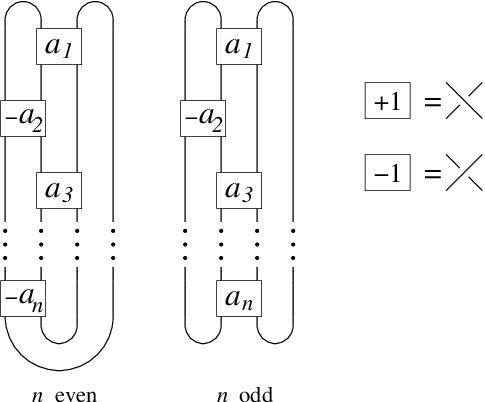
A link in is two-bridge if and only if it has a planar diagram of the form shown in Figure 7. Such links are classified up to isotopy by pairs of relatively prime integers modulo the relation if or . The integers are the coefficients in a continued fraction expansion for :
| (63) |
(If , the link is the unlink, and is defined to be .) We write to denote the two-bridge link determined by the pair . If is odd, is a knot, while if is even, it is a two-component link, both of whose components are unknots. Finally,
It is easy to see that the diagram of Figure 7 is alternating if and only if all the ’s have the same sign. If , it is well known that admits a continued fraction expansion of the type shown in equation (63) with all . Thus any two-bridge knot or link can be represented by an alternating two-bridge diagram.
Lemma 5.1.
Let be an alternating two-bridge diagram representing . Then the links obtained by resolving the top crossing of in both possible ways are and .
Proof.
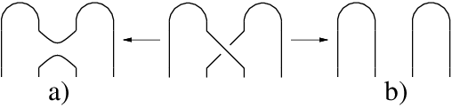
By hypothesis, is an alternating diagram, so all the ’s have the same sign. Without loss of generality, we assume that they are all positive. If we resolve the top crossing as in Figure 8a, then we can untwist the remaining twists in the central column, move the rightmost strand all the way to the left, and flip the whole diagram over to obtain a two-bridge diagram with continued fraction expansion . We have
| (64) |
so .
On the other hand, if the top crossing is resolved as in Figure 8b and , then we obviously have a two-bridge diagram with continued fraction expansion . Thus
| (65) |
so .
Finally, if the resolution is as in Figure 8b and , then we undo the twists in the top left of the resolved diagram and are left with a two-bridge diagram with continued fraction expansion . Here we have
| (66) |
so .
∎
Definition 5.2.
A special singular two-bridge link is a singular link obtained by replacing the top crossing of an alternating two-bridge diagram with a singular crossing.
Theorem 5.3.
Suppose is either a two-bridge knot or link or a special singular two-bridge link and that . Then is -thin (with respect to either component) for all .
Remark: The condition rules out the unlink, which we have already seen is not thin.
Proof.
By induction on . For the base case, we must consider links and singular links with . There is a unique regular two-bridge link with determinant , namely the unknot, so the claim is easily verified in this case. Now suppose is a singular link. The unoriented resolution is a two-bridge diagram of a knot with determinant , so it must be the unknot. Moreover is alternating, and it is well known that any alternating diagram of the unknot is nugatory — it can be reduced to the standard diagram by repeated application of the Reideimester I move. Thus is twist-equivalent to the singular link illustrated in Figure 2. By Corollary 4.12, it suffices to show that is -thin.
is clearly symmetric, so without loss of generality, we assume that the marked component belongs to the side labeled . By Lemma 3.2, we have
| (67) |
and the Poincaré polynomial is
| (68) |
On the other hand,
| (69) |
so . Since is the unlink, which has both determinant and signature equal to , we see that . It follows that is -thin.
We now assume the theorem holds for links with determinant . Given a regular two-bridge link , we choose an alternating two-bridge diagram representing , and let and denote the links obtained by taking the oriented and singular resolutions of its topmost crossing, so that , , and fit into a skein exact sequence. is clearly a special singular two-bridge link, and is a two-bridge link by Lemma 5.1. Combining Lemmas 2.3 and 5.1, we see that one of has determinant and the other has determinant . Thus both and are -thin by the induction hypothesis, and
| (70) |
Then Theorem 4.7 implies that is -thin as well.

Next, suppose we are given a special singular two-bridge link with determinant . We distinguish two cases, depending on the orientation of the singular crossing. First, suppose that the crossing is oriented as in Figure 9a or its reverse. Then as shown in the figure, is twist-equivalent to a diagram with just the singular crossing in the top block. The unoriented resolution is a two-bridge link with continued fraction expansion , where all the ’s have the same sign. Suppose for the moment that , so . There is a skein exact sequence relating , , and , where the continued fraction expansions of and are and . Thus
| (71) |
and
| (72) |
In other words,
| (73) | ||||
| (74) | ||||
| (75) |
so . The induction hypothesis implies that both and are -thin, so by Theorem 4.7, we conclude that is -thin as well. The argument when is identical, except that we replace with .
We now consider the case where the singular crossing is oriented as in Figure 9b or its reverse. We claim that without loss of generality, we may assume . Indeed, suppose this is not the case. Then as indicated in the figure, is twist-equivalent to a singular two-bridge knot with continued fraction expansion . As in the previous case, all the ’s have the same sign; we assume for the moment that .
In this case, we consider the skein exact sequence relating , , and . Let , where has continued fraction expansion . The unoriented resolution has continued fraction expansion , so . On the other hand, has continued fraction expansion . Since , it follows that . Thus , and is -thin. Finally, when , we argue as above, but with replaced by . This completes the proof of the theorem.
∎
5.2. Other Knots
Theorem 4.7 and Corollary 4.12 can also be applied on a case-by-case basis to show that certain other knots are thin. For example, we have the following
Criterion 5.4.
Suppose and are two knots related by a crossing change, and that
| (76) | ||||
| (77) |
Then if and the oriented resolution are -thin , is -thin as well.

Proof.
We have
| (78) | ||||
| (79) |
so if and have the same phase, . It follows that
| (80) | ||||
| (81) |
so two applications of Theorem 4.7 give the desired result. ∎
This criterion provides a fast and reasonably effective way of finding thin knots with small crossing number. Figure 10 shows diagrams of five -crossing knots to which the criterion can be applied. Combining with the results of Theorem 1, we see that the only knots with 8 crossings or fewer which are not known to be -thin () are , and . Of these, the knot (the torus knot) cannot be -thin for any , since its HOMFLY polynomial is not alternating. (Of course, it is not thin for either.) It seems quite plausible that the remaining three knots are thin, although we do not have any proof of this fact.
Interestingly, there also exist alternating knots whose HOMFLY polynomials are nonalternating, although they are somewhat harder to find. The smallest such knot is (Knotscape numbering). It has HOMFLY polynomial
which is alternating except at the final term. This knot cannot be -thin for any , but its ordinary Khovanov homology is thin by Lee’s theorem.
5.3. Unreduced Homology
So far, we have been concerned only with the reduced version of the Khovanov-Rozansky homology. We conclude by briefly considering to the problem of computing the unreduced homology. Here, unfortunately, our methods are less successful. Nonetheless, combining our knowledge of the reduced homology with a theorem of Gornik [6] enables us to compute the unreduced homology in a few special cases. The first ingredient in the calculation is a spectral sequence relating the two theories.
Lemma 5.5.
There is a spectral sequence with term which converges to . All of its differentials respect the -grading.
Proof.
Let be the edge operator corresponding to the component . The action of on induces a filtration where . From property (4) of 3.1 it follows that for . The homology of is , so the term of the associated spectral sequence is . Finally the fact that the differentials in this spectral sequence respect the -grading merely reflects the fact that the same is true in . ∎
We will also need Gornik’s generalization of Lee’s spectral sequence to the Khovanov-Rozansky homology [6].
Theorem 5.6.
(Gornik) Let be a knot. There is a spectral sequence with term which converges to a vector space of dimension supported in homological grading . The differential lowers the -grading by .
Proposition 5.7.
Let be the positive torus knot. For , the Poincaré polynomial of is given by
| (82) |
where as usual
| (83) |
Proof.
The HOMFLY polynomial of is given by
| (84) |
and , so
| (85) |
In other words, is generated by classes () and (), with homological gradings and respectively. In particular, there is one generator in grading and in each of the gradings .
Consider the generators in the term of the spectral sequence of Lemma 5.5. They have homological grading , so they can only be killed by generators of the form . Since the differentials in this spectral sequence respect the -grading, it is not difficult to check that the only possible differential from to takes to . We claim that this differential must be nontrivial. Indeed, suppose it were not. Then the term of Gornik’s spectral sequence would contain the generator , which must be killed by some generator with homological grading , and the grading of this element would be at least greater than the -grading of . But the generator in grading with largest -grading is , and its -grading is only greater than that of . Thus we have arrived at a contradiction.
It follows that in homological grading , has generators (). In Gornik’s spectral sequence, these must be killed by the generators (). In particular, all of these generators must survive in the reduced-unreduced spectral sequence, so there are no differentials from to . To finish the proof, we simply repeat this argument, considering differentials from to , then from to , and so on. ∎
References
- [1] D. Bar-Natan. On Khovanov’s categorification of the Jones polynomial. Alg. Geom. Top., 2:337–370, 2002.
- [2] D. Bar-Natan and J. Green. FastKh and JavaKh. in Mathematica package KnotTheory. Available at http://katlas.math.toronto.edu, 2005.
- [3] J. S. Carter and M. Saito. Reidemeister moves for surface isotopies and their interpretation as moves to movies. J. Knot Theory Ramifications, 2:251–284, 1993.
- [4] J. H. Conway. An enumeration of knots and links, and some of their algebraic properties. In Computational Problems in Abstract Algebra (Proc. Conf., Oxford, 1967), pages 329–358. Pergamon, Oxford, 1970.
- [5] N. Dunfield, S. Gukov, and J. Rasmussen. The superpolynomial for knot homologies. math.GT/0505662, 2005.
- [6] B. Gornik. Note on Khovanov link cohomology. math.QA/0402266, 2004.
- [7] V. F. R. Jones. On knot invariants related to some statistical mechanical models. Pacific J. Math., 137:311–334, 1989.
- [8] M. Khovanov. A categorification of the Jones polynomial. Duke Math. J., 101:359–426, 2000.
- [9] M. Khovanov. Patterns in knot cohomology. I. Experiment. Math., 12:365–374, 2003.
- [10] M. Khovanov and L. Rozansky. Matrix factorizations and link homology. math.QA/0401268, 2004.
- [11] M. Khovanov and L. Rozansky. Matrix factorizations and link homology II. math.QA/0505056, 2005.
- [12] E. S. Lee. The support of Khovanov’s invariants for alternating knots. math.GT/0201105, 2002.
- [13] H. Murakami, T. Ohtsuki, and S. Yamada. Homfly polynomial via an invariant of colored plane graphs. Enseign. Math. (2), 44:325–360, 1998.
- [14] K. Murasugi. Knot theory and its applications. Birkhäuser Boston Inc., Boston, MA, 1996. Translated from the 1993 Japanese original by Bohdan Kurpita.
- [15] J. Rasmussen. Khovanov homology and the slice genus. math.GT/04020131, 2004.
- [16] A. Shumakovitch. Khoho. Available at http://www.geometrie.ch/KhoHo/, 2003.
- [17] V. G. Turaev. The Yang-Baxter equation and invariants of links. Invent. Math., 92:527–553, 1988.