A better proof of the Goldman–Parker conjecture

Richard Evan Schwartz Address: Department of Mathematics, University of MarylandCollage Park, MD 20742, USA Email: res at math dot brown dot edu

Abstract

The Goldman–Parker Conjecture classifies the complex hyperbolic $C$ –reflection ideal triangle groups up to discreteness. We proved the Goldman–Parker Conjecture in [6] using a rigorous computer-assisted proof. In this paper we give a new and improved proof of the Goldman–Parker Conjecture. While the proof relies on the computer for extensive guidance, the proof itself is traditional.

keywords

Hyperbolic, complex reflection group, ideal triangle group, Goldman–Parker conjecture

\nocolon

\urladdr

http://www.math.brown.edu/ res/

\primaryclass

20F67 \secondaryclass20F65, 20F55

$\cal G\mskip-2.0mu$ eometry & $\cal T\!\!$ opology $\cal G$ $\cal G$ $\cal G$ $\cal G$ $\cal G$ $\cal G$ $\cal G$ $\cal G$ $\cal G$ $\cal G$ $\cal G$ $\cal G$ $\cal G$ $\cal G$ $\cal G$ $\cal T$ $\cal T$ $\cal T$ $\cal T$ $\cal T$ $\cal T$ $\cal T$ $\cal T$ $\cal T$ $\cal T$ $\cal T$ $\cal T$ $\cal T$ $\cal T$ $\cal T$ Volume 9 (2005) 1539–1601\nlPublished: 10 August 2005

\thetitle

\theauthors

\theaddress

\cl

Email:\stdspace\theemail

\cl

URL:\stdspace\theurl

Abstract

\theabstract

AMS Classification numbers Primary: \theprimaryclass

Secondary: \thesecondaryclass

Keywords: \thekeywords

Proposed: Benson Farb Received: 8 February 2005\nlSeconded: David Gabai, Martin Bridson Revised: 2 July 2005

1 Introduction

Let $\mbox{\boldmath{$H$}}^{2}$ be the hyperbolic plane. Let $G$ denote the usual reflection ideal triangle group acting on $\mbox{\boldmath{$H$}}^{2}$ . The standard generators of $G$ are $\iota_{0},\iota_{1},\iota_{2}$ .

$PU(2,1)$ is the holomorphic isometry group of $\mbox{\boldmath{$C$}}\mbox{\boldmath{$H$}}^{2}$ , the complex hyperbolic plane. See Section 2 for more details. A $C$ –reflection is an order $2$ element of $PU(2,1)$ which is conjugate to the element which has the action $(z,w)\to(z,-w)$ . A complex hyperbolic ideal triangle group representation is a representation of $G$ which maps the generators to $C$ –reflections, and the products of pairs of generators to parabolic elements. Let ${\rm Rep\/}(G)$ denote the set of such representations, modulo conjugacy. It turns out that ${\rm Rep\/}(G)$ is a half-open interval, naturally parametrized by $s\in[0,\infty)$ . See Section 2.

Define

\underline{s}=\sqrt{105/3};\hskip 30.0pt\overline{s}=\sqrt{125/3};

(1)

In [5], Goldman and Parker introduced ${\rm Rep\/}(G)$ (using different notation) and proved that $\rho_{s}$ is a discrete embedding if $s\in[0,\underline{s}]$ . They conjectured that $\rho_{s}$ is a discrete embedding iff $\rho_{s}(\iota_{0}\iota_{1}\iota_{2})$ is not an elliptic element of $PU(2,1)$ . This corresponds to parameters $s\in[0,\overline{s}]$ . We took care of the interval $(\underline{s},\overline{s}]$ in [6], using a rigorous computer-assisted proof, together with some new constructions in complex hyperbolic geometry. However, the proof in [6] is extremely complicated and requires massive computations.

The purpose of this paper is to give a new and improved proof of the Goldman–Parker Conjecture. Our new proof is based on an idea we worked out, to a limited extent, in [7, Sections 8–10]. To each of the three generators $I_{j,s}=\rho_{s}(\iota_{j})$ we will associate an piecewise analytic sphere $\Sigma_{j,s}$ . We call $\Sigma_{j,s}$ a loxodromic $R$ –sphere. Our construction is such that $I_{j,s}(\Sigma_{j,s})=\Sigma_{j,s}$ and that $I_{j,s}$ interchanges the two components of $S^{3}-\Sigma_{j,s}$ . The key step in our argument is showing that $\Sigma_{i,s}\cap\Sigma_{j,s}$ is a contractible set—the union of $2$ arcs arranged in a ‘T’ pattern—for $i\not=j$ , and that $\Sigma_{j,s}$ is embedded. This sets up a version of the familiar ping-pong lemma, and it follows readily from this picture that $\rho_{s}$ is a discrete embedding.

In [7, Sections 8–10] we established the intersection and embedding properties of our spheres for all $s\in[\overline{s}-\epsilon,\overline{s})$ , using a perturbative argument. However, we couldn’t get an effective estimate on $\epsilon$ back then. Here, in Section 3, we develop a theory for loxodromic $R$ –spheres and use it to establish the two desired properties for all $s\in[\underline{s},\overline{s})$ . Pictures like Figure 4.2 indicate that our construction works for all $s\in[0,\overline{s})$ . However, there are certain technical details we could not overcome when trying to deal with parameters outside the range $[\underline{s},\overline{s})$ .

We wrote a Java applet which illustrates this paper in great detail and, in particular, lets the reader plot pictures like Figure 4.2 for all parameter values. The paper is independent of the applet, but the applet greatly enhances the paper because it lets the reader see visually the objects we refer to here mainly with symbols. We encourage the reader to use the applet while reading the paper. One can access the applet from my website. The applet provides massive hands-on evidence that our construction works for all $s\in[0,\overline{s}]$ . In fact, most of our proof works for all $s\in[0,\overline{s}]$ but there are certain technical estimates we rely on that do not hold over the whole range of parameters.

Since I wrote [6] $7$ years ago, there has been considerable development of complex hyperbolic discrete groups. Some of us feel that all the new technology—eg, [1], [7], [3], [8]—should reprove the Goldman–Parker Conjecture without too much pain. Nonetheless, a new proof has never appeared and I thought that this paper would be of interest. Also, I never liked my proof in [6] and have wanted a better proof for a long time.

This paper divides into $2$ halves. The first half is organized like this:

•

Section 2: background;
•

Section 3: theory of loxodromic $R$ –spheres;
•

Section 4: the proof.

The proof requires a handful of technical estimates, which we make in Sections 5–7.

The technical estimates all concern the location in $S^{3}$ of a certain collection of arcs of circles. There is a $1$ –parameter family of these arcs and one can readily compute their positions numerically. You can see from my applet (or from your own experiments) that these estimates hold by a wide margin and are blatantly true for parameters in $[\underline{s},\overline{s}]$ . The original version of this paper had computer-aided estimates on the locations of these arcs. At the request of the referee of this paper, these computer-aided proofs have been replaced with analytic calculations.

The analytic calculations done in the paper are in part based on a brilliant algebraic idea due to the anonymous¹¹ 1 Eventually I guessed that the referee was John Parker. You can tell the lion by his claw. referee. The idea can be summarized by saying that one should introduce the parameter

x=\frac{e^{2}+|e|^{2}+\overline{e}^{2}}{1-|e|^{2}}

and then write all relevant quantities in terms of $x$ . (See subsections 5.1–5.2 for details.) Here $e$ (which is not to be confused with the base of the natural log) is one of the coordinates of an eigenvector of the word $\rho(\iota_{1}\iota_{0}\iota_{2})$ .

I would like to thank Elisha Falbel, Bill Goldman and John Parker for many conversations, over the years, about complex hyperbolic geometry. Also, I would like to thank the University of Maryland, the Institute for Advanced Study, the National Science Foundation (Grant DMS-0305047) and the John Simon Guggenheim Memorial Foundation, for their generous support.

2 Background

2.1 Complex hyperbolic geometry

[2] and [4] are good references for complex hyperbolic geometry. [8] also has a good introduction.

2.1.1 The ball model

$\mbox{\boldmath{$C$}}^{2,1}$ is a copy of the vector space $\mbox{\boldmath{$C$}}^{3}$ equipped with the Hermitian form

\langle u,v\rangle=u_{1}\overline{v}_{1}+u_{2}\overline{v}_{2}-u_{3}\overline{v}_{3}

(2)

$\mbox{\boldmath{$C$}}\mbox{\boldmath{$H$}}^{2}$ and its ideal boundary are respectively the projective images, in the complex projective plane $\mbox{\boldmath{$C$}}\mbox{\boldmath{$P$}}^{2}$ , of

N_{-}=\{v\in\mbox{\boldmath{$C$}}^{2,1}|\ \langle v,v\rangle<0\};\hskip 15.0ptN_{0}=\{v\in\mbox{\boldmath{$C$}}^{2,1}|\ \langle v,v\rangle=0\}

(3)

(The set $N_{+}$ has a similar definition.) The projectivization map

(v_{1},v_{2},v_{3})\to(v_{1}/v_{3},v_{2}/v_{3})

(4)

takes $N_{-}$ and $N_{0}$ respectively to the open unit ball and unit sphere in $\mbox{\boldmath{$C$}}^{2}$ . Henceforth we identify $\mbox{\boldmath{$C$}}\mbox{\boldmath{$H$}}^{2}$ with the open unit ball. $\mbox{\boldmath{$C$}}\mbox{\boldmath{$H$}}^{2}$ is called the complex hyperbolic plane. It is a symmetric space of negative curvature.

2.1.2 Slices

There are two kinds of totally geodesic $2$ –planes in $\mbox{\boldmath{$C$}}\mbox{\boldmath{$H$}}^{2}$ :

•

The $R$ –slices are $2$ –planes, $PU(2,1)$ –equivalent to $\mbox{\boldmath{$R$}}\mbox{\boldmath{$H$}}^{2}=\mbox{\boldmath{$R$}}^{2}\cap\mbox{\boldmath{$C$}}\mbox{\boldmath{$H$}}^{2}$ .
•

The $C$ –slices are $2$ –planes, $PU(2,1)$ –equivalent to $\mbox{\boldmath{$C$}}\mbox{\boldmath{$H$}}^{1}=\mbox{\boldmath{$C$}}\mbox{\boldmath{$H$}}^{2}\cap\mbox{\boldmath{$C$}}^{1}$ .

Let $F$ stand either for $R$ or $C$ . The accumulation set on $S^{3}$ , of an $F$ –slice, is called an $F$ –circle. An $F$ –reflection is an involution in ${\rm Isom\/}(\mbox{\boldmath{$C$}}\mbox{\boldmath{$H$}}^{2})$ whose fixed point set is an $F$ –circle. The map $(z,w)\to(z,-w)$ is a prototypical $C$ –reflection and the map $(z,w)\to(\overline{z},\overline{w})$ is a prototypical $R$ –reflection. The $F$ –slice determines the $F$ –reflection and conversely.

2.1.3 Isometries

$SU(2,1)$ is the $\langle,\rangle$ preserving subgroup of $SL_{3}(\mbox{\boldmath{$C$}})$ , the special complex linear group. $PU(2,1)$ is the projectivization of $SU(2,1)$ . Elements of $PU(2,1)$ act isometrically on $\mbox{\boldmath{$C$}}\mbox{\boldmath{$H$}}^{2}$ and are classified according to the usual scheme for groups acting on negatively curved spaces. Loxodromic elements move every point of $\mbox{\boldmath{$C$}}\mbox{\boldmath{$H$}}^{2}$ greater than some $\epsilon>0$ ; elliptic elements fix a point in $\mbox{\boldmath{$C$}}\mbox{\boldmath{$H$}}^{2}$ ; and the remaining elements are parabolic.

We now discuss $C$ –reflections in more detail. Given a vector $C\subset N_{+}$ we define

I_{C}(U)=-U+\frac{2\langle U,C\rangle}{\langle C,C\rangle}C.

(5)

$I_{C}$ is an involution fixing $C$ and $I_{C}\in SU(2,1)$ . See [4, page 70]. The element of $PU(2,1)$ corresponding to $I_{C}$ is a $C$ –reflection. Every $C$ –reflection is conjugate to the map $(z,w)\to(z,-w)$ discussed above. $C$ –reflections are also called complex reflections.

2.2 Heisenberg space

2.2.1 Basic definitions

In the ball model, $\mbox{\boldmath{$C$}}\mbox{\boldmath{$H$}}^{2}$ is a ball sitting inside complex projective space $\mbox{\boldmath{$C$}}\mbox{\boldmath{$P$}}^{2}$ . For this discussion we fix some $p\in S^{3}$ , the ideal boundary of $\mbox{\boldmath{$C$}}\mbox{\boldmath{$H$}}^{2}$ . There exists a complex projective automorphism $\beta$ of $\mbox{\boldmath{$C$}}\mbox{\boldmath{$P$}}^{2}$ which maps $p$ to a point in $\mbox{\boldmath{$C$}}\mbox{\boldmath{$P$}}^{2}-\mbox{\boldmath{$C$}}^{2}$ and which identifies $\mbox{\boldmath{$C$}}\mbox{\boldmath{$H$}}^{2}$ with the Siegel domain:

Z=\{(z_{1},z_{2})|\ 2{\rm Re\/}(z_{1})<-|z_{2}|^{2}\}\subset\mbox{\boldmath{$C$}}^{2}\subset\mbox{\boldmath{$C$}}\mbox{\boldmath{$P$}}^{2}

(6)

We write $\infty=\beta(p)$ in this case. The isometries of $\mbox{\boldmath{$C$}}\mbox{\boldmath{$H$}}^{2}$ which fix $\infty$ act as complex linear automorphisms of $Z$ . The set $\partial Z$ is characterized as the set of null vectors relative to the Hermitian form

\langle u,v\rangle^{\prime}=u_{1}\overline{v}_{3}+u_{2}\overline{v}_{2}+u_{3}\overline{v}_{1}.

(7)

We call $\cal H$ $=\mbox{\boldmath{$C$}}\times\mbox{\boldmath{$R$}}$ Heisenberg space. $\cal H$ is equipped with a group law:

(\zeta_{1},t_{1})\cdot(\zeta_{2},t_{2})=(\zeta_{1}+\zeta_{2},t_{1}+t_{2}+2{\rm Im\/}(\overline{\zeta}_{1}\zeta_{2}))

(8)

There is a natural map from $\partial Z$ to $\cal H$ , given by

\mu(z_{1},z_{2})=(\frac{z_{2}}{\sqrt{2}},{\rm Im\/}(z_{1})).

(9)

The inverse map is given by

(z,t)\to(-|z|^{2}+it,z\sqrt{2}).

(10)

A Heisenberg stereographic projection from $p$ is a map $\mbox{\boldmath{$B$}}\co S^{3}-\{p\}\to\cal H$ of the form $\mu\circ\beta$ where $\beta$ is as above. We write $\infty=\mbox{\boldmath{$B$}}(p)$ in this case. We will somewhat abuse terminology and speak of elements of $PU(2,1)$ acting on $\cal H$ . We mean that the conjugate of an element, by Heisenberg stereographic projection, acts on $\cal H$ . If such a map stabilizes $\infty$ , it acts as an affine map of $\cal H$ .

•

The $C$ –circles in $\cal H$ which contain $\infty$ all have the form $(\{z\}\times\mbox{\boldmath{$R$}})\cup\infty$ . The remaining $C$ –circles are ellipses which project to circles in $C$ . The plane containing the ellipse is the contact plane based at the center of mass of the ellipse. See below for more detail.
•

The $R$ –circles which contain $\infty$ are straight lines. One of these $R$ –circles is $(\mbox{\boldmath{$R$}}\times\{0\})\cup\infty$ . The bounded $R$ –circles in $\cal H$ are such that their projections to $C$ are lemniscates.

2.2.2 The contact distribution

The set of complex lines tangent to $S^{3}$ forms a $PU(2,1)$ –invariant contact distribution on $S^{3}$ . The $R$ –circles are tangent to this distribution and the $C$ –circles are transverse to it. The image of the contact distribution, under Heisenberg stereographic projection, is a contact distrubition on $\cal H$ . It is defined as the kernel of the $1$ form $dt+2(xdy-ydx)$ , when points in $\cal H$ are written as $(x+iy,t)$ . Compare [4, page 124], Any element of $PU(2,1)$ acting on $\cal H$ respects this contact distribution. Each plane in the distribution is called a contact plane.

Area Principle\quaSuppose $\alpha$ is a piecewise smooth curve in ${\cal H\/}$ , tangent to the contact distribution, such that $\pi(\alpha)$ is a closed loop. Then the height difference—meaning the difference in the $t$ –coordinates—between the two endpoints of $\alpha$ is $4$ times the signed area of the compact region enclosed by $\pi(\alpha)$ . This is basically Green’s theorem. Compare [4, Section 4]. Call this principle the area principle.

2.3 Spinal spheres

2.3.1 Basic definitions

Basic information about bisectors and spinal spheres can be found in [4]. Here we recall some of the basics.

A bisector is a subset of $\mbox{\boldmath{$C$}}\mbox{\boldmath{$H$}}^{2}$ of the form $\{x\in\mbox{\boldmath{$C$}}\mbox{\boldmath{$H$}}^{2}|\ d(x,p)=d(x,q)\}$ . Here $p\not=q$ are two distinct points in $\mbox{\boldmath{$C$}}\mbox{\boldmath{$H$}}^{2}$ and $d$ is the complex hyperbolic metric. A spinal sphere is the ideal boundary of a bisector. Every two spinal spheres are equivalent under $PU(2,1)$ , even though this is not immediately obvious. Equivalently, a spinal sphere is any set of the form

\mbox{\boldmath{$B$}}^{-1}((\mbox{\boldmath{$C$}}\times\{0\})\cup\infty).

Here $B$ is a Heisenberg stereographic projection. Thus,

S=(\mbox{\boldmath{$C$}}\times\{0\})\cup\infty

is a model in $\cal H$ for a spinal sphere. From the second definition we see some of the structure of spinal spheres. Here are some objects associated to $S$ :

•

$S$ has a singular foliation by $C$ –circles. The leaves are given by $C_{r}\times\{0\}$ where $C_{r}$ is a circle of radius $r$ centered at the origin. The singular points are $0$ and $\infty$ . We call this the $C$ –foliation.
•

$S$ has a singular foliation by $R$ –circles. The leaves are horizontal lines through the origin. The singular points are again $0$ and $\infty$ . We call this the $R$ –foliation.
•

The singular points $0$ and $\infty$ are called the poles of $S$ .
•

The spine of $S$ is defined as the $C$ –circle containing the poles. In our case, the spine is $(\{0\}\times\mbox{\boldmath{$R$}})\cup\infty$ . Note that the spine of $S$ only intersects $S$ at the singular points.

Any other spinal sphere inherits this structure, by symmetry. The two foliations on a spinal sphere look like lines of lattitude and longitude on a globe. A spinal sphere is uniquely determined by its poles. Two spinal spheres are cospinal if they have the same spine.

2.3.2 Generic tangencies with spinal spheres

In this section we prove a useful technical result about how an $R$ –circle intersects a spinal sphere. Let $\pi\co{\cal H\/}\to\mbox{\boldmath{$C$}}$ be projection. The next result is illustrated in Figure 2.1.

Lemma 2.1.

Let $S=(\mbox{\boldmath{$C$}}\times\{0\})\cup\infty$ as above. Let $\gamma$ be a finite $R$ –circle in $\cal H$ . Suppose

•

$\gamma$ is tangent to $S$ at $p\not=0$ .
•

The line $L\subset\mbox{\boldmath{$C$}}$ , containing $0$ and $\pi(p)$ , is not tangent to $\pi(\gamma)$ at the double point of $\pi(\gamma)$ .

Then $\gamma$ has first but not second order contact with $S$ . Moreover, a neighborhood of $p$ in $\gamma$ lies on one side of $S$ .

Proof.

Since $\gamma$ is tangent to $S$ at $p$ , and $\gamma$ is also tangent to the contact distribution, and the contact distribution is not tangent to $S$ at $p$ , we see that $\gamma$ is tangent to the $R$ –circle of $S$ which contains $p$ . This $R$ –circle is exactly $L\times\{0\}$ . But then $L$ is tangent to $\pi(\gamma)$ at $\pi(p)$ . Figure 2.1 shows the situation when a lobe of $\pi(\gamma)$ surrounds $0$ . The other topological possibility has the same proof. The basic idea of the proof is that $L$ does not have second order contact with $\pi(\gamma)$ at $\pi(p)$ , by convexity.

We first apply the area principle to the integral curve $\alpha$ made from two horizontal line segments and a portion of $\gamma$ , so that $\pi(\alpha)$ bounds the lightly shaded region $A$ shown in Figure 2.1. From the area principle we see that the height of $q$ is positive, and also a quadratic function of the Euclidean distance from $\pi(q)$ to $\pi(p)$ . The quadratic dependence comes from the strict convexity of $\pi(\gamma)$ in a neighborhood of $\pi(p)$ .

A similar argument works when we take the relevant integral curve which projects to the region $A\cup B$ . We see that the height of the point $r$ is positive, and also a quadratic function of the Euclidean distance from $\pi(r)$ to $\pi(p)$ . Now we know that points on $\gamma$ , on either side of $p$ , rise quadratically up and away from $S$ . ∎

Corollary 2.2.

Suppose $\gamma$ links the spine of a spinal sphere $\Sigma$ and $\gamma$ is tangent to $\Sigma$ at some point $p$ . Then $\gamma$ has first but not second order contact with $\Sigma$ at $p$ and a neighborhood of $p$ in $\gamma$ lies to one side of $\Sigma$ .

Proof.

When we normalize so that $\Sigma=S$ . then the spine of $\Sigma$ projects to $0$ . One of the lobes of $\pi(\gamma)$ surrounds $0$ , and $p$ projects to some nonzero point. In short, we have the picture in Figure 2.1, and the hypotheses of the previous result are forced. ∎

2.4 Equations for $C$ –circles

Suppose that $C$ is a $C$ –circle in ${\cal H\/}$ which links $\{0\}\times\mbox{\boldmath{$R$}}$ . Let $\pi\co{\cal H\/}\to\mbox{\boldmath{$C$}}$ be projection as above. Then $\pi(C)$ is a circle in $C$ which surrounds $0$ . As in [7, section 2] we study $\Psi_{*}(C)$ , where $\Psi_{*}$ is the map

\Psi_{*}(z,t)=(\arg z,t).

(11)

Define

r={\rm radius\/}(\pi(C));\qquad d=|{\rm center\/}(\pi(C))|;\qquad A=(r/d)^{2}.

(12)

We only define $A$ when $d>0$ . We call $A$ the aspect of $C$ . Note that $A>1$ .

Lemma 2.3.

Let $A$ be the aspect of $C$ . Up to scaling and rotation $\Psi_{*}(C)$ is the graph of

f_{A}(t)=\sin(t)(\cos(t)+\sqrt{A-\sin^{2}(t)})

(13)

Proof.

We normalize so that $(1,0)$ is the center of mass of $C$ . Then $d=1$ and $C$ is contained in the contact plane through $(1,0)$ . This plane is spanned by $(1,0)$ and $(i,2)$ . Let $C_{\theta}$ be the point on $C$ such that the line through $0$ and $\pi(C_{\theta})$ makes an angle of $\theta$ with the $x$ axis. Then $\Psi_{*}(C)$ is the graph of the function $\theta\to{\rm height\/}(C_{\theta})=2y$ , where $C_{\theta}=(x,y)$ . Our formula comes from solving the equations $(x-1)^{2}+y^{2}=r^{2}$ and $x=y\cot(\theta)$ in terms of $y$ . ∎

Lemma 2.4.

If $A\geq 9$ then $f_{A}^{\prime\prime}$ is negative on $(0,\pi)$ and positive on $(\pi,2\pi)$ .

Proof.

We compute that

\frac{d}{dA}f^{\prime\prime}_{A}(t)=\frac{A(2-A+\cos(2t))\sin(t)}{2(A-\sin^{2}(t))^{5/2}}=g_{A}(t)\sin(t),

(14)

where $g_{A}(t)<0$ . Hence $\frac{d}{dA}f^{\prime\prime}_{A}$ is negative on $(0,\pi)$ and positive on $(\pi,2\pi)$ . We just need to prove that $f^{\prime\prime}_{9}$ is negative on $(0,\pi)$ and positive on $(\pi,2\pi)$ . We compute that $f_{9}^{\prime\prime}(\pi/2)=-7/\sqrt{8}<0$ . Thus, we just need to see that $f_{9}^{\prime\prime}(t)=0$ only at $t=0$ and $t=\pi$ . Setting $u=\cos(t)$ we compute²² 2 We differentiate the function $\sin(t)(\cos(t)+\sqrt{(A-1)+\cos^{2}(t)}),$ which is a re-writing of $f_{A}$ , using Mathematica [10].

f_{9}^{\prime\prime}=\frac{-4h(u)\sin(t)}{(8+u^{2})^{3/2}};\hskip 15.0pth(u)=14+12u^{2}+u^{4}+8u\sqrt{8+u^{2}}+u^{3}\sqrt{8+u^{2}}.

(15)

For $u\in(-1,1]$ we have

h(u)\geq 14+12u^{2}+u^{4}+24u+3u^{3}=(1+u)(14+10u+2u^{2}+u^{3})>0.

This shows that $f_{9}^{\prime\prime}(t)\not=0$ if $t\not\in\{0,\pi\}$ . ∎

Remark\quaThe preceding lemma is essentially the same as Lemma 4.11 of [3], with the variable change $\phi=t+\pi/2$ .

2.5 Ideal triangle groups

2.5.1 The basic definition

We will use the same set-up as in [6]. Given $s\in[0,\infty)$ we define

\beta_{s}=\frac{s+i}{\sqrt{2+2s^{2}}}.

(16)

Sometimes we write $\beta$ instead of $\beta_{s}$ , when the dependence is clear. As we showed in [6], every ideal triangle in $S^{3}$ is conjugate to a triangle with vertices

p_{0}=(\beta,\overline{\beta});\qquad p_{1}=(\beta,\beta);\qquad p_{2}=(\overline{\beta},\overline{\beta}).

(17)

In brief, the idea is that we can apply an element of $PU(2,1)$ so that all three vertices of our ideal triangle lie on the Clifford torus

\{(z,w)|\ |z|=|w|\}\subset S^{3}

and then we can rotate the Clifford torus until the points are as above.

Let $I_{j}$ be the $C$ –reflection which fixes $p_{j-1}$ and $p_{j+1}$ . We compute that the elements $I_{0},I_{1},I_{2}$ are given by

\left[\matrix{0&-1&0\cr-1&0&0\cr 0&0&-1}\right];\quad\left[\matrix{-1&0&0\cr 0&3&-4\overline{\beta}\cr 0&4\beta&-3}\right];\quad\left[\matrix{3&0&-4\beta\cr 0&-1&0\cr 4\overline{\beta}&0&-3}\right],

(18)

Letting $g_{0}=I_{1}I_{0}I_{2}$ we compute

g_{0}=\left[\matrix{0&-1&0\cr-A_{1}&0&A_{2}\cr-A_{2}&0&-\overline{A}_{1}}\right];\hskip 15.0ptA_{1}=\frac{s+17i}{s+i};\quad A_{2}=\frac{12\sqrt{2}i}{\sqrt{1+s^{2}}}.

(19)

A direct computation, for example using the result on [4, page 201], shows that $g$ is loxodromic for $s\in[0,\overline{s})$ and parabolic for $\overline{s}$ . See [5].

As we mentioned in the introduction, we are mainly interested in the case when $s\in(\underline{s},\overline{s}]$ , though many of our constructions work for $s\in[0,\underline{s}]$ as well. Actually, we will carry out most of our constructions for $s\in(\underline{s},\overline{s})$ , because there are now several good discreteness proofs for the case $\overline{s}$ . See [7] and [3].

2.5.2 Some associated objects

When $s<\overline{s}$ , the element $g_{0}$ is loxodromic. In this case $g_{0}$ stabilizes a pair $(E_{0},Q_{0})$ , where $E_{0}$ is a $C$ –circle containing the fixed points of $g_{0}$ and $Q_{0}$ is an arc of $E_{0}$ bounded by the two fixed points. Of the two possible arcs, we choose $Q_{0}$ so that it varies continuously with the parameter and shrinks to a point as $s\to\overline{s}$ . The curve

\rho_{0}=\{(u\beta,\overline{u}\overline{\beta})|\ u\in S^{1}\}

(20)

is an $R$ –circle fixed by the map $(z,w)=(\overline{w},\overline{z})$ . This map interchanges $p_{1}$ and $p_{2}$ and fixes $p_{0}$ . In short $\rho_{0}$ is an $R$ –circle of symmetry for our configuration.

One can define $Q_{1}$ , $Q_{2}$ , etc. by cycling the indices mod $3$ . The objects

(C_{j},E_{j},p_{j},Q_{j});\qquad j=0,1,2.

(21)

are the elementary objects of interest to us. Figure 2.3 shows those of the objects which lie on the Clifford torus, when the Clifford torus is drawn as a square torus (in “arg-arg coordinates”). The black dots are the points of $E_{0}\cap\rho_{0}$ .

3 Loxodromic $R$ –spheres

3.1 The cospinal foliation

Our constructions are all based on the pair $(E_{0},Q_{0})$ from subsection 2.5, though we could take any pair $(E_{0},Q_{0})$ and make the same definitions. Again, $E_{0}$ is a $C$ –circle and $Q_{0}$ is a proper arc of $E_{0}$ . Note that $Q_{0}$ determines $E_{0}$ uniquely. We include $E_{0}$ in our notation for emphasis.

Let $p,q\in E_{0}$ be two distinct points. The pair $(p,q)$ is harmonic with respect to $(E_{0},Q_{0})$ if the geodesic connecting $p$ to $q$ in $\mbox{\boldmath{$C$}}\mbox{\boldmath{$H$}}^{2}$ is perpendicular to the geodesic connecting the endpoints of $Q_{0}$ . (Both these geodesics lie in the $C$ –slice bounded by $E_{0}$ .) A spinal sphere $S$ is harmonic w.r.t. $(E_{0},Q_{0})$ if the poles of $S$ lie in $E_{0}$ and are harmonic w.r.t $(E_{0},Q_{0})$ . An $R$ –arc $\alpha$ is harmonic w.r.t. $(E_{0},Q_{0})$ if the endpoints of $\alpha$ are harmonic w.r.t. $(E_{0},Q_{0})$ . Every harmonic $R$ –arc is contained in a harmonic spinal sphere.

•

Let $S(E_{0},Q_{0})$ denote the union of all spinal spheres which are harmonic with respect to $(E_{0},Q_{0})$ . We call $S(E_{0},Q_{0})$ the cospinal foliation.
•

Let $R(E_{0},Q_{0})$ denote the union of all $R$ –arcs which are harmonic with respect to $(E_{0},Q_{0})$ .
•

Let $G(E_{0},Q_{0})\subset PU(2,1)$ denote the group which fixes the endpoints of $Q_{0}$ . Then $G(E_{0},Q_{0})$ acts transitively the elements in $S(E_{0},Q_{0})$ and simply transitively on the elements of $R(E_{0},Q_{0})$ .

To see a picture we work in ${\cal H\/}$ and normalize so that $E_{0}=(\{0\}\times\mbox{\boldmath{$R$}})\cup\infty$ and $Q_{0}$ is the unbounded arc whose endpoints are $(0,\pm 1)$ . We call this standard position. In this case $(p,q)$ is harmonic with respect to $(E_{0},Q_{0})$ iff $p=(0,r)$ and $q=(0,r^{-1})$ . We include the possibility that $r=0$ , so that $r^{-1}=\infty$ . All the spinal spheres of interest to us are bounded in $\cal H$ , except for $(\mbox{\boldmath{$C$}}\times\{0\})\cup\infty$ , which corresponds to the case $r=0$ .

Lemma 3.1.

Every bounded spinal sphere in $S(E_{0},Q_{0})$ is a convex surface of revolution.

Proof.

All such spinal spheres are surfaces of revolution, by symmetry. Moreover, all such spinal spheres are affine images of the so-called unit spinal sphere, which has poles $(0,\pm 1)$ . The unit spinal sphere satisfies the equation $|z|^{4}+t^{2}=1$ and hence is convex. See [4, page 159]. Being affine images of a convex set, the other spinal spheres of interest to us are also convex. ∎

Lemma 3.2.

Every two distinct spinal spheres in $S(E_{0},Q_{0})$ are disjoint.

Proof.

Let $S_{1}$ and $S_{2}$ be two distinct spinal spheres in $S(E_{0},Q_{0})$ . Using the action of $G(E_{0},Q_{0})$ we can arrange that $S_{1}=(\mbox{\boldmath{$C$}}\times\{0\})\cup\infty$ and that the endpoints of $S_{2}$ are $(r,0)$ and $(r^{-1},0)$ , with $r\not=0$ . But then $S_{2}$ lies either entirely in the upper half space, or entirely the lower half space. In either case $S_{2}$ is disjoint from $S_{1}$ . ∎

3.2 Loxodromic $R$ –cones and $R$ –spheres

Given $x\in S^{3}-E_{0}$ there is a unique element $\alpha\in R(E_{0},Q_{0})$ such that $x\in\alpha$ . We let $\Sigma(E_{0},Q_{0};x)$ denote the portion of $\alpha$ which connects $x$ to a point in $Q_{0}$ . Given a subset $S\subset S^{3}-E_{0}$ we define

\Sigma(E_{0},Q_{0};S)=\bigcup_{x\in S}\Sigma(E_{0},Q_{0};x).

(22)

We call $\Sigma(E_{0},Q_{0};S)$ the loxodromic cone on $S$ .

Let $C_{1}$ be a $C$ –circle which links $E_{0}$ . Technical Lemma I (Lemma 4.1) establishes this linking property when $(C_{1},E_{0})$ are as in subsection 2.5.) Let $(E_{2},Q_{2})=I_{1}(E_{0},Q_{0})$ . Here $I_{1}$ is the $C$ –reflection fixing $C_{1}$ . We say that a loxodromic $R$ –sphere is an object of the form

\Sigma_{1}=\Sigma(E_{0},Q_{0};C_{1})\cup\Sigma(E_{2},Q_{2};C_{1})

(23)

If the $C$ –slice bounded by $C_{1}$ is perpendicular to the $C$ –slice bounded by $E_{0}$ then $C_{1}$ lies in one of the elements of $S(E_{0},Q_{0})$ and $\Sigma_{1}$ is a spinal sphere. In general $\Sigma_{1}$ is not a spinal sphere. In Section 4 we will show that the loxodromic $R$ –spheres of interest to us are embedded spheres but not spinal spheres.

We are interested in the case when $\Sigma_{1}$ is not a spinal sphere. Henceforth we assume that $\Sigma_{1}$ is not a spinal sphere. In this case we call $\Sigma_{1}$ generic.

Lemma 3.3.

Let $\Sigma_{1}$ be a generic $R$ –sphere. There exists a unique $R$ –circle $R_{1}$ such that $R_{1}$ intersects $E_{0},C_{1},E_{2}$ each in two points. Also, $R_{1}\subset\Sigma_{1}$ and the $R$ –reflection in $R_{1}$ is a symmetry of $\Sigma_{1}$ . We call $R_{1}$ the $R$ –axis of $\Sigma_{1}$ .

Proof.

We put $(E_{0},Q_{0})$ in standard position. Recall that $G(E_{0},Q_{0})$ is the stabilizer subgroup of $Q_{0}$ which preserves the endpoints. Using the action of $G(E_{0},Q_{0})$ we can normalize so that the center of mass of $C_{1}$ is $(r,0)$ for some $r>0$ . Consider the $R$ –circle $R_{1}=(\mbox{\boldmath{$R$}}\times\{0\})\cup\infty$ . By symmetry $R_{1}$ intersects $C_{1}$ twice. Also $R_{1}$ intersects $E_{0}$ twice. Finally, we have $I_{1}(R_{1})=R_{1}$ by symmetry. Hence $R_{1}$ intersects $E_{2}$ twice. The $R$ –reflection $J_{1}$ in $R_{1}$ is an anti-holomorphic element preserving $(E_{0},Q_{0})$ and $C_{1}$ , and hence a symmetry of $\Sigma_{1}$ . If there was some other axis $R^{\prime}_{1}$ then the composition of the $R$ –reflection symmetries $J_{1}$ and $J_{1}^{\prime}$ would a non-trivial element of $PU(2,1)$ preserving both $(E_{0}.Q_{0})$ and $C_{1}$ . But no such element exists. Hence $R_{1}$ is unique. ∎

3.3 The elevation map

The set $R(E_{0},Q_{0})$ is topologically a cylinder. Since $G(E_{0},Q_{0})$ acts transitively on $R(E_{0},Q_{0})$ , this cylinder admits a natural family of flat metrics. Put another way, we can write $R(E_{0},Q_{0})=\mbox{\boldmath{$R$}}/2\pi\mbox{\boldmath{$Z$}}\times\mbox{\boldmath{$R$}}$ . The identification is unique up to post-composition with a map of the form $(x,y)\to(x+a,by+c)$ . That is, the identification is unique up to affine maps.

There is a tautological map $\Psi_{0}\co S^{3}-E_{0}\to R(E_{0},Q_{0})$ defined as follows: $\Psi_{0}(x)$ is the element of $R(E_{0},Q_{0})$ which contains $x$ . If we identify $R(E_{0},Q_{0})$ with $\mbox{\boldmath{$R$}}/2\pi\times\mbox{\boldmath{$R$}}$ then we have nice coordinates for this map. Given $x\in S^{3}-E$ we let $\widehat{x}$ be a lift of $x$ . We define

\Psi_{0}(x)=\left(\arg\frac{\langle\widehat{x},\widehat{E}_{0}\rangle}{\sqrt{\langle\widehat{x},\widehat{Q}_{1}\rangle\langle\widehat{x},\widehat{Q}_{2}\rangle}},\log\bigg|\frac{\langle\widehat{x},\widehat{Q}_{1}\rangle}{\langle\widehat{x},\widehat{Q}_{2}\rangle}\bigg|\right)

(24)

Here $\widehat{Q}_{1}$ and $\widehat{Q}_{2}$ are lifts of the endpoints of $Q_{0}$ and $\widehat{E}_{0}$ is a polar vector of $E_{0}$ . This is to say that $\langle\widehat{E}_{0},\widehat{Y}\rangle=0$ whenever $\widehat{Y}$ is a lift of a point $Y\in E_{0}$ .

Remarks\qua

(i)\quaIt is possible to choose a well-defined branch of the square root in Equation 24. This is basically a topological fact, deriving from the fact that the map

f(x)\to\langle\widehat{x},\widehat{Q}_{1}\rangle\langle\widehat{x},\widehat{Q}_{2}\rangle

induces the map on homology

f_{*}\co\mbox{\boldmath{$Z$}}=H_{1}(S^{3}-E_{0})\to H_{1}(\mbox{\boldmath{$C$}}-\{0\})=\mbox{\boldmath{$Z$}}

which is multiplication by $2$ .

(ii)\quaDifferent choices of lifts lead to maps which differ by post-composition with affine maps.

(iii)\quaTo see that Equation 24 works as claimed we compute that $\Psi_{0}$ conjugates $G(E_{0},Q_{0})$ to isometries of $\mbox{\boldmath{$R$}}/2\pi\times\mbox{\boldmath{$R$}}$ . The point here is that $(\widehat{Q}_{1},\widehat{Q}_{2},\widehat{E}_{0})$ is an eigenbasis for the elements of $G(E_{0},Q_{0})$ .

Henceforth we set $\Psi=\Psi_{0}$ . Note that $\Psi(x)=\Psi(y)$ iff $x$ and $y$ belong to the same element of $R(E_{0},Q_{0})$ . $\Psi$ maps the orbit $G(E_{0},Q_{0})(x)$ diffeomorphically onto $\mbox{\boldmath{$R$}}/2\pi\mbox{\boldmath{$Z$}}\times\mbox{\boldmath{$R$}}$ . hence $d\Psi$ has rank $2$ everywhere.

For any $x\in S^{3}-E_{0}$ let $\Pi_{x}$ denote the contact plane at $x$ . Let

L_{x}=d\Psi(\Pi_{x})

(25)

As we just mentioned, $d\Psi$ has full rank at at $x$ but $d\Psi$ maps the $3$ –dimensional vector space $T_{x}(S^{3})$ onto a $2$ –dimensional tangent space. The kernel of $d\Psi$ is the vector tangent to the element of $R(E_{0},Q_{0})$ through $x$ . This kernel is therefore contained in $\Pi_{x}$ . Hence $L_{x}$ is a line. The following result captures some of the basic features of this situation.

Lemma 3.4.

Let $\gamma$ be an $F$ –circle and let $x\in\gamma-E_{0}$ be a point.

•

If $\mbox{\boldmath{$F$}}=\mbox{\boldmath{$R$}}$ and $\gamma$ is not tangent to $\Sigma(E_{0},Q_{0};x)$ then $\Psi(\gamma)$ is a nonsingular curve at $\Psi(x)$ and the tangent line is $L_{x}$ .
•

If $\mbox{\boldmath{$F$}}=\mbox{\boldmath{$C$}}$ then $\Psi(\gamma)$ is nonsingular at $\Psi(x)$ and transverse to $L_{x}$ .

Proof.

When $\gamma$ is an $R$ –circle, the tangent vector $v$ to $\gamma$ at $x$ lies in $\Pi_{x}$ but is not contained in the kernel of $d\Psi_{x}$ . Part 1 of our lemma follows from this fact. When $\gamma$ is a $C$ –circle, $v\not\in\Pi_{x}$ and hence $d\Psi_{x}(v)\not\in L_{x}$ . ∎

Remark\quaAt this point, the reader anxious to see our main construction should skip to Section 4.

3.4 More details on slopes

From Lemma 3.4 we see that $L_{x}$ tells us a great deal about what $\Psi$ does to $R$ –circles and $C$ –circles. We now investigate this further. Let $\sigma_{x}$ denote the slope of $L_{x}$ . Of course $\sigma_{x}$ depends on our choice of normalization, but the general statements we make are independent of normalization. Let $S_{0}$ denote the spinal sphere whose poles are $\partial Q_{0}$ .

Lemma 3.5.

If $x\in S_{0}$ then $L_{x}$ is a vertical line and hence $\sigma_{x}$ is infinite. Otherwise $\sigma_{x}$ is finite and nonzero.

Proof.

Let $H\subset G(E_{0},Q_{0})$ denote the $1$ –parameter subgroup consisting of the pure loxodromic elements. These elements do not twist at all in the direction normal to the slice bounded by $E_{0}$ . By symmetry $\Psi$ maps the orbit $H(x)$ to a vertical line in $\mbox{\boldmath{$R$}}/2\pi\mbox{\boldmath{$Z$}}\times\mbox{\boldmath{$R$}}$ . On the other hand $H(x)$ is tangent to $\Pi_{x}$ iff $x\in S_{0}$ . From this we see that $\sigma_{x}$ is infinite iff $x\in S_{0}$ . Now $\Psi$ maps the $C$ –circles foliating the spinal spheres in $S(E_{0},Q_{0})$ to horizontal lines. From this fact, and from Lemma 3.4, we see that $\sigma_{x}\not=0$ .

Lemma 3.6.

Let $x,y\in S^{3}-E_{0}$ . Then $\sigma_{x}=\sigma_{y}$ iff $x$ and $y$ lie in the same $G(E_{0},Q_{0})$ orbit.

Proof.

By symmetry we have $\sigma_{x}=\sigma_{y}$ if $x$ and $y$ are $G(E_{0},Q_{0})$ equivalent. We just have to establish the converse. Each $x\in S^{3}-E_{0}$ determines a $1$ –parameter subgroup $H_{x}\subset G(E_{0},Q_{0})$ which has the property that the orbit $H_{x}(x)$ is integral to the contact structure. Then $\Psi$ maps $H_{x}(x)$ to a geodesic on $\mbox{\boldmath{$R$}}/2\pi\mbox{\boldmath{$Z$}}\times\mbox{\boldmath{$R$}}$ which is tangent to $L_{x}$ . It suffices to show that $H_{x}\not=H_{y}$ if $x$ and $y$ lie in different $G(E_{0},Q_{0})$ orbits. Suppose, for the sake of contradiction, that there are $G(E_{0},Q_{0})$ –inequivalent $x,y$ for which $H_{x}=H_{y}$ . Using the action of $G(E_{0},Q_{0})$ we can arrange that $\Psi(x)=\Psi(y)$ . Let $h\in H_{x}=H_{y}$ . By symmetry we have $\Psi(h(x))=h(y)$ . But then we can make a closed quadrilateral, $\cal Q$ as follows:

•

One side of $\cal Q$ is the portion of $H_{x}(x)$ which connects $x$ to $h(x)$ .
•

One side of $\cal Q$ is the portion of $H_{y}(y)$ which connects $y$ to $h(y)$ .
•

One side of $\cal Q$ is $\Sigma(E_{0},Q_{0};y)-\Sigma(E_{0},Q_{0};x)$ .
•

One side of $\cal Q$ is $\Sigma(E_{0},Q_{0};h(y))-\Sigma(E_{0},Q_{0};h(x))$ .

Here we are choosing $x,y$ so that $\Sigma(E_{0},Q_{0};x)\subset\Sigma(E_{0},Q_{0};y)$ . The shaded region in Figure 3.1 is the projection of $\cal Q$ to $C$ .

We normalize so that $(E_{0},Q_{0})$ is the standard pair and $x=(r,0)$ and $y=(s,0)$ . If we choose $h$ close to the identity, then $\pi(\cal Q)$ projects to an embedded quadrilateral in $C$ , as suggested by Figure 3.1. The point here is that the fibers of $\Psi$ are lobes of lemniscates which have their double points at the origin. Since $\cal Q$ is integral to the contact structure, and yet a closed loop, we contradict the Area Principle of subsection 2.2.2. ∎

Corollary 3.7 (Slope Principle).

Let $\gamma_{1},\gamma_{2}\in S^{3}-E_{0}$ be two $R$ –arcs such that $\Psi(\gamma_{1})$ and $\Psi(\gamma_{2})$ are nonsingular at a point $x\in\mbox{\boldmath{$R$}}/2\pi\mbox{\boldmath{$Z$}}\times\mbox{\boldmath{$R$}}$ , and tangent to each other at $x$ . Then $\gamma_{1}$ and $\gamma_{2}$ intersect at some point $y\in\Psi^{-1}(x)$ .

Proof.

Each fiber of $\Psi$ , including $\Psi^{-1}(x)$ , intersects each orbit of $G(E_{0},Q_{0})$ in one point. Our result now follows from Lemma 3.4 and Lemma 3.6. ∎

We normalize $\Psi$ so that $\sigma_{x}$ is positive when $S_{0}$ separates $Q_{0}$ from $x$ . In this case we call $x$ remote from $Q_{0}$ . Thus we can say that $\sigma_{x}\in(0,\infty)$ iff $x$ is remote from $S_{0}$ .

3.5 Images of $C$ –circles

Lemma 3.8.

Suppose $C$ is a $C$ –circle which links $E_{0}$ . Then $\Psi(C)$ is the graph of a function $\psi\co\mbox{\boldmath{$R$}}/2\pi\mbox{\boldmath{$Z$}}\to\mbox{\boldmath{$R$}}$ .

Proof.

$\Psi(C)$ is a smooth loop by Lemma 3.4. We need to prove that $\Psi(C)$ is never vertical. Let $C=C_{1}\cup C_{2}$ , where $C_{1}$ is the closure of the remote points of $C$ and $C_{2}$ is the complement. Let $I$ be a $C$ –reflection in a $C$ –circle contained in $S_{0}$ . Then $I$ interchanges the two components of $S^{3}-S_{0}$ , and $\Psi$ conjugates $I$ to a reflection in a horizontal line of $\mbox{\boldmath{$R$}}/2\pi\mbox{\boldmath{$Z$}}\times\mbox{\boldmath{$R$}}$ . (This is seen by choosing $\widehat{Q}_{1}$ and $\widehat{Q}_{2}$ in Equation 24 so that these vectors are swapped by $I$ .) Hence $\Psi(I(C_{2}))$ is the image of $\Psi(C_{2})$ reflected in a horizontal line. By symmetry, then, it suffices to show that $\Psi(C_{1})$ is never vertical.

Let $x\in C_{1}$ . We normalize so that $(E_{0},Q_{0})$ is the standard pair and $x=(r,0)$ for some $r>0$ . Since $C$ links $E$ , we can parameterize $C$ as $C(\theta)=(z(\theta),t(\theta))$ , where $\theta$ is the angle between the ray connecting $0$ to $\pi(C(\theta))$ and $R$ . We are interested in $q=C(0)$ .

If $t^{\prime}(0)=0$ then $C$ is tangent to $S=(\mbox{\boldmath{$C$}}\times\{0\})\cup\infty$ at $q$ . But $S$ is a member of $S(E_{0},Q_{0})$ . Hence $\Psi(C)$ is horozontal at $\Psi(C(0))$ . Conversely, if $\Psi(C)$ is horizontal at $\Psi(C(0))$ then $C$ is tangent to $S$ and hence $t^{\prime}(0)=0$ .

If $t^{\prime}(0)>0$ then $w=d\Psi_{q}(C^{\prime}(0))$ lies in the interior of the cone bounded by the $x$ –axis and $L_{C(0)}$ , a line whose slope is either positive or infinite. (The idea here is that the statement holds when the center of mass of $C$ is near $(0,0)$ , and then Lemma 3.4 and the linking condition guarantee that the cone condition holds no matter how $C$ varies.) Hence $w$ is not vertical.

If $t^{\prime}(0)<0$ then the projection to $C$ of the fiber of $\Psi$ which contains $C(\epsilon)$ curves down and clockwise, as shown in Figure 3.2. But then the horizontal component of $w=d\Psi_{q}(\gamma^{\prime}(0))$ exceeds $1$ because the angle $\delta$ in Figure 3.2 exceeds the angle $\epsilon$ . Again $w$ is not vertical. ∎

We say that $C$ generically links $E_{0}$ if the $C$ –slice bounded by $C$ is not perpendicular to the $C$ –slice bounded by $E_{0}$ .

Lemma 3.9.

Suppose that $C$ is a $C$ –circle which generically links $E_{0}$ . Then $\Psi(C)$ is the graph of a function $\psi\co S^{1}\to\mbox{\boldmath{$R$}}$ which has one maximum and one mimimum.

Proof.

Since $C$ generically links $E_{0}$ the image $\Psi(C)$ is not contained in a horizontal line. The $\Psi$ –preimages of horizontal lines are spinal spheres. Since $C$ is not contained in any of these spinal spheres, $C$ can intersect each of them at most twice. Hence $\Psi(C)$ intersects each horizontal line at most twice. Our result follows immediately. ∎

Corollary 3.10.

Suppose that $C_{1}$ generically links $E_{0}$ . Then $\Sigma(E_{0},Q_{0};C_{1})$ is an embedded topological disk, analytic away from $C_{1}\cup Q_{0}$ .

Proof.

The set $\Sigma(E_{0},Q_{0};C_{1})-Q_{0}$ is foliated by $R$ –arcs of the form $\gamma(\theta)$ , where $\theta\in C_{1}$ is a point. Two arcs $\gamma(\theta_{1})$ and $\gamma(\theta_{2})$ are disjoint because $\Psi(\gamma(\theta_{j}))=\Psi(\theta_{j})$ and $\Psi(\theta_{1})\not=\Psi(\theta_{2})$ . Moreover, the arcs vary analytically. Hence $\Sigma(E_{0},Q_{0};C_{1})-Q_{0}$ is homeomorphic to an annulus (with one boundary component deleted) and analytic away from $C_{1}$ .

There is a map $f\co C_{1}\to Q_{0}$ given as follows: $f(x)$ is defined to be the endpoint of $\Sigma(E_{0},Q_{0};x)$ . If $f(C_{1})$ is more than one point—as it is when $C$ generically links $E_{0}$ —then $f$ is generically $2$ to $1$ and $1$ to $1$ at exactly two points. This follows from Lemma 3.9. Thus, $f$ has the effect of folding $C_{1}$ in half over an arc of $Q_{0}$ . Hence the $R$ –arcs foliating $\Sigma(E_{0},Q_{0};C_{1})$ intersect $Q$ in pairs, with two exceptions. Topologically, $\Sigma(E_{0},Q_{0};C_{1})$ is obtained from an annulus by gluing the inner circle together by a folding map, as in Figure 3.3. From this description we see that $\Sigma(E_{0},Q_{0};C_{1})$ is an embedded disk, analytic off of $Q_{0}$ . ∎

3.6 Images of linked $R$ –circles

Lemma 3.11.

Let $\gamma$ be an $R$ –circle which links $E_{0}$ . Then $\gamma$ is tangent to exactly two spinal spheres in $S(E_{0},Q_{0})$ .

Proof.

We normalize so that $(E_{0},Q_{0})$ is in standard position. Let $Q_{t}$ denote the unbounded $C$ –arc whose endpoints are $(0,\pm(1+t))$ . Then $Q_{t}$ exits every compact subset of $\cal H$ as $t\to\infty$ . Let $N(t)$ denote the number of elements of $S(E_{0},Q_{t})$ which are tangent to $\gamma$ .

We define $S(E_{0},Q_{\infty})$ to be the collection of spinal spheres of the form $(\mbox{\boldmath{$C$}}\times\{s\})\cup\infty$ . Given this definition we can define $N(\infty)$ to be the number of spinal spheres in $S(E_{0},Q_{\infty})$ tangent to $\gamma$ . Let’s analyze $N(\infty)$ first. Let $\pi\co{\cal H\/}\to\mbox{\boldmath{$C$}}$ be projection. Suppose $\gamma$ is tangent to a horizontal spinal sphere $S_{s}=(\mbox{\boldmath{$C$}}\times\{s\})\cup\infty$ at $x$ . Since $\gamma$ is also tangent to the contact plane $\Pi_{x}$ , we see that $\gamma$ is tangent to the line $\Pi_{x}\cap S_{s}$ . But $\Pi_{x}\cap S_{s}$ is a horizontal line which intersects $E_{0}$ . Hence $\pi(\gamma)$ is tangent at $\pi(x)$ to a line through the origin. But $\pi(\gamma)$ is a lemniscate, one of whose lobes surrounds the origin. See Figure 2.1. Hence there are only $2$ lines through the origin which are tangent to $\pi(\gamma)$ . Hence $N(\infty)=2$ .

Now fix some value of $t$ . Since $\gamma$ links $E_{0}$ , Corollary 2.2 applies: If $\gamma$ is tangent to a spinal sphere $S$ of $\Sigma(E_{0},Q_{t})$ then $\gamma$ locally lies to one side of $S$ and has first but not second order contact with $S$ . Moreover, as $t^{\prime}\to t$ , the spinal spheres of $S(E_{0},Q_{t^{\prime}})$ converge smoothly to the spinal spheres of $S(E_{0},Q_{t})$ . These two properties imply that the tangency points vary continuously with $t$ and cannot be created or destroyed as $t$ changes. The two properties also hold at $t=\infty$ .

From the discussion in the preceding paragraph we see that $N(t)$ is independent of $t$ . Since $N(\infty)=2$ we also have $N(1)=2$ . ∎

Corollary 3.12 (Elevation Image).

Suppose that $\gamma$ is an $R$ –circle which links $E_{0}$ . Then $\Psi(\gamma)$ is the union of two non-singular arcs, each having nonzero slope at every point. The two non-singular arcs meet at two cusp points.

Proof.

Everything but the statement about the cusps follows from Lemma 3.4, Lemma 3.5, and Lemma 3.11. The two cusps appear because $\gamma$ locally lies on one side of each of the two spinal spheres to which it is tangent. ∎

3.7 Linking of the poles

As above $I_{1}(E_{0},Q_{0})=(E_{2},Q_{2})$ , where $I_{1}$ is the $C$ –reflection fixing the $C$ –circle $C_{1}$ which generically links $E_{0}$ . Also $R_{1}$ is the $R$ –axis of the $R$ –sphere $\Sigma_{1}$ given in Equation 23.

Lemma 3.13.

$E_{0}$ and $E_{2}$ are linked.

Proof.

We normalize so that $(E_{0},Q_{0})$ is the standard pair and the center of mass of $C_{1}$ is $(r,0)$ for some $r>0$ . Then $R_{1}=(\mbox{\boldmath{$R$}}\times\{0\})\cup\infty$ . Let $A_{1}\subset R_{1}$ be the bounded interval whose endpoints are $C_{1}\cap R_{1}$ . The center of $A_{1}$ is $(r,0)$ . Since $C_{1}$ links $E_{0}$ , we have $0\in A_{1}$ . Since the center of $A_{1}$ is positive, $0$ lies in the left half of $A_{1}$ . Now $I_{1}|_{R_{1}}$ acts as a linear fractional transformation interchanging $A_{1}$ with $R_{1}-A_{1}$ . But then $I_{1}(0,0)=(s,0)$ with $s<0$ and $I_{1}(\infty)=(r,0)$ with $r>0$ . The two points of $E_{2}\cap R_{1}$ are $I_{1}(0,0)$ and $I_{1}(\infty)$ . But these points separate $(0,0)$ from $\infty$ on $R_{1}$ . Hence $E_{2}$ and $E_{0}$ are linked. ∎

$\Psi(C_{1})$ and $\Psi(E_{2})$ have some symmetry: Let $J_{1}$ be the $R$ –reflection fixing $R_{1}$ . Then $\Psi$ conjugates $J_{1}$ to an isometric $180$ degree rotation of $\mbox{\boldmath{$R$}}/2\pi\mbox{\boldmath{$Z$}}\times\mbox{\boldmath{$R$}}$ . The fixed point set of this rotation is exactly $\Psi(R_{1}-E_{0})$ , which is a pair of points on the same horizontal level and $\pi$ units around from each other. This rotation is a symmetry of $\Psi(C_{1})$ and also of $\Psi(E_{2})$ . Figure 3.4 shows a picture of the three possibilities.

We say that $\Sigma_{1}$ is interlaced if the picture looks like the right hand side. That is, a vertical line separates the minimum of $\Psi(E_{2})$ from the minimum of $\Psi(C_{1})$ . When we normalize the interlaced case as above, $(0,0)$ separates the center of mass of $C_{1}$ from the center of mass of $E_{2}$ . From this we see that the set of interlaced $R$ –spheres is connected. In the interlaced case, the interlacing pattern of the extrema of $\Psi(C_{1})$ and $\Psi(E_{2})$ forces

\Psi(C_{1})\cap\Psi(E_{2})=\Psi(R_{1}-E_{0}).

(26)

3.8 The Two Cusp Lemma

We say that an $R$ –circle $\widehat{\gamma}$ is affiliated with $\Sigma(E_{0},Q_{0};C_{1})$ if $\widehat{\gamma}$ contains an $R$ –arc of the form $\Sigma(E_{0},Q_{0};x)$ , for $x\in C_{1}$ , but $\widehat{\gamma}$ is not the $R$ –axis $R_{1}$ of $\Sigma_{1}$ . The purpose of this section is to prove the following result.

Lemma 3.14 (Two Cusp).

Suppose that $\Sigma_{1}$ is interlaced. Suppose that $\widehat{\gamma}$ is an $R$ –circle affiliated to $\Sigma(E_{2},Q_{2};C_{1})$ . Then $\Psi(\widehat{\gamma})$ . is the union of two nonsingular arcs, each of which has everywhere nonzero slope. The two arcs are joined at two cusps.

The Two Cusp Lemma is an immediate consequence of Lemma 3.15 below and the Elevation Image Lemma.

Lemma 3.15.

Suppose that $\Sigma_{1}$ is interlaced. Then every $R$ –circle affiliated to $\Sigma(E_{0},q_{0};C_{1})$ links $E_{2}$ .

Proof.

By symmetry, every $R$ –circle affiliated to $\Sigma(E_{0},q_{0};C_{1})$ links $E_{2}$ if and only if every $R$ –circle affiliated to $\Sigma(E_{2},Q_{2};C_{1})$ links $E_{0}$ .

Let $\widehat{\gamma}$ be an $R$ –circle affiliated to $\Sigma(E_{2},Q_{2};C_{1})$ . We claim that that $\widehat{\gamma}\cap E_{0}=\emptyset$ . Once we know this, we see that either all affiliates of $\Sigma(E_{2},Q_{2};C_{1})$ link $E_{0}$ or all affiliates fail to link $E_{0}$ . By continuity, the link/unlink option is independent of the choice of interlaced $R$ –sphere. We check explicitly, for one interlaced $R$ –sphere—eg, the one in Figure 4.5—that the link option holds for some of the affiliates. Hence the link option always holds.

It remains to establish our claim. By symmetry $\widehat{\gamma}^{\prime}=I_{C_{1}}(\gamma)$ is affiliated with $\Sigma(E_{0},Q_{0};C_{1})$ . By construction, $\Psi(\gamma^{\prime}-E_{0})$ is a single point of $\Psi(C_{1})$ and $\Psi(\gamma^{\prime}-E_{0})\in\Psi(R_{1}-E_{0})$ iff $R^{\prime}=R_{1}$ . The point is that $\Psi$ is injective on $C_{1}$ . Therefore

\Psi(\gamma^{\prime}-E_{0})\cap\Psi(R_{1}-E_{0})=\emptyset.

(27)

We have by hypotheses and Equation 26 that

\Psi(\gamma^{\prime}-E_{0})\cap\Psi(E_{2})\subset\Psi(C_{1})\cap\Psi(E_{2})=\Psi(R_{1}-E_{0}).

(28)

Combining Equations 27 and 28 we have

\Psi(\gamma^{\prime}-E_{0})\cap\Psi(E_{2})=\emptyset.

(29)

Hence $(\gamma^{\prime}-E_{0})\cap E_{2}=\emptyset$ . Since $E_{0}\cap E_{2}=\emptyset$ we conclude that $\widehat{\gamma}^{\prime}\cap E_{2}=\emptyset$ . Hence $\widehat{\gamma}\cap E_{0}=\emptyset$ . This establishes our claim. ∎

3.9 Asymmetry

Let $\Delta_{0}$ denote the $C$ –slice which bounds $E_{0}$ . Let $S_{0}$ denote the spinal sphere whose poles are $Q_{0}$ . Let $R_{1}$ denote the $R$ –axis of the $R$ –sphere $\Sigma_{1}$ given in Equation 23. Again recall that $I_{1}(E_{0},Q_{0})=(E_{2},Q_{0})$ . We we will assume explicitly that $E_{1}$ and $E_{2}$ are generically linked. Hence $E_{i}$ and $E_{j}$ are also generically linked.

Let $\eta\co S^{3}\to\Delta_{0}$ denote orthogonal projection. The generic linking condition implies that $\eta(E_{j})$ is a circle (rather than a point) for $j=1,2$ . Let $\Theta_{1}=\eta(E_{0})$ . For $j=0,2$ let $\Theta_{j}$ be the circle which is perpendicular to $\eta(E_{j})$ and contains the endpoints of $\eta(Q_{j})$ . Note that $\Theta_{0}$ and $\Theta_{1}$ intersect at right angles, since $\Theta_{0}=\eta(S_{0})$ and $\Theta_{1}=\eta(E_{0})$ .Some of these objects are drawn in Figure 3.5. Say that $\Sigma_{1}$ is asymmetric if $\Theta_{0}\cap\Theta_{1}\cap\Theta_{2}=\emptyset$ . This is the generic case. The goal of this section is to prove:

Lemma 3.16 (Asymmetry Lemma).

Suppose $\Sigma_{1}$ is asymmetric and interlaced. Let $x,y\in E_{2}$ be two points which are harmonic with respect to $Q_{2}$ . Then $\Psi(x)$ and $\Psi(y)$ lie on the same horizontal line in $\mbox{\boldmath{$R$}}/2\pi\mbox{\boldmath{$Z$}}\times\mbox{\boldmath{$R$}}$ iff $x,y\in R_{1}$ .

Proof.

We first list some basic properties of the map $\eta$ .

•

$\eta(E_{0})$ is the boundary of $\Delta_{0}$ and $\eta(Q_{0})$ is an arc of $\eta(E_{0})$ . This follows from the fact that $\eta$ is the identity on $E_{0}$ .
•

If $C$ is a $C$ –circle which is disjoint from $E_{0}$ then $\eta(C)$ is a circle contained in the interior of $E_{0}$ . The restriction of $\eta$ to $C$ is a linear fractional transformation. This property comes from the fact that $\eta$ is holomorphic on complex lines.
•

If $S$ is a spinal sphere whose spine is $E_{0}$ , then $\eta(S)$ is a geodesic in $\Delta_{0}$ . In particular, $\gamma_{0}=\eta(S_{0})$ is the geodesic whose endpoints are $\eta(Q_{0})$ . Indeed, an alternate definition of a spinal sphere is the preimage of such a geodesic under $\eta$ . See [4].
•

$\eta$ maps each spinal sphere in the cospinal foliation to geodesics perpendicular to $\eta(S_{0})$ . This follows from symmetry: namely that $\eta$ conjugates $G(E_{0}.Q_{0})$ to isometries of $\Delta_{0}$ which fix both endpoints of $\eta(Q_{0})$ .
•

$\eta$ maps the $R$ –axis of $\Sigma_{1}$ to a geodesic $\gamma_{1}$ which is simultaneously perpendicular to $\eta(S_{0})$ and $\eta(C_{1})$ and $\eta(Q_{2})$ . Again this follows from symmetry: The $R$ –reflection in the $R$ –axis of $\Sigma_{1}$ preserves both $C_{1}$ and $Q_{2}$ . Indeed, the isometric reflection in $\gamma_{1}$ stabilizes $\eta(Q_{0})$ and $\eta(Q_{2})$ and $\eta(C_{1})$ and $\Delta_{0}$ .

Remark\quaThe reader can see all these properties in action using my Applet.

Now we turn to the main argument in the proof of the Asymmetry Lemma. If $x,y\in R_{1}$ then $\Psi(x)$ and $\Psi(y)$ are precisely the two symmetry points of $\Psi(E_{2})$ and $\Psi(C_{1})$ discussed in Lemma 3.15, and then $\Psi(x)$ and $\Psi(y)$ lie on the same horizontal line.

Suppose, conversely, that $\Psi(x)$ and $\Psi(y)$ lie on the same horizontal line. This means that $\eta(x)$ and $\eta(y)$ lie on the same geodesic $\gamma$ of $\Delta_{0}$ , where $\gamma$ is perpendicular to both $\Theta_{0}$ and $\Theta_{1}$ . By assumption $x,y\in E_{2}$ are harmonic with respect to $Q_{2}$ . Since the restriction of $\eta$ to $E_{2}$ is a linear fractional transformation, the points $\eta(x)$ and $\eta(y)$ are in harmonic position with respect to $\eta(Q_{2})$ . So, we conclude that the geodesic $\gamma$ has the following properties:

•

$\gamma$ is perpendicular to $\Theta_{0}$ since $\gamma$ is a geodesic.
•

$\gamma$ is perpendicular to $\gamma_{0}$ , the geodesic connecting the endpoints of $\gamma(Q_{0})$ . Hence $\gamma$ is perpendicular to $\Theta_{1}$ .
•

$\gamma$ intersects $\eta(E_{2})$ in two points which are in harmonic position with respect to $\eta(Q_{2})$ . But then $\gamma$ is perpendicular to $\Theta_{2}$ , the circle which is perpendicular to $\eta(E_{2})$ and contains $\eta(Q_{2})$ in its endpoints.

Figure 3.5 shows a picture. The lemma below says that there is only one geodesic which has this property, and this geodesic is $\gamma_{1}=\eta(R_{1})$ . Hence $\Psi(x)$ and $\Psi(y)$ lie on the same horizontal line as $\Psi(R_{1}-E_{0})$ . This forces $x,y\in R_{1}$ . ∎

Lemma 3.17.

Let $\Theta_{0},\Theta_{1},\Theta_{2}$ be $3$ circles in $\mbox{\boldmath{$C$}}\cup\infty$ . Suppose that $\Theta_{0}\cap\Theta_{1}$ is a pair of points and $\Theta_{0}\cap\Theta_{1}\cap\Theta_{2}=\emptyset$ . Then there is at most one circle which is simultaneously perpendicular to $\Theta_{j}$ for $j=0,1,2$ .

Proof.

We normalize by a Moebius transformation so that $\Theta_{0}$ and $\Theta_{1}$ are lines through the origin. Then a circle in $C$ is perpendicular to $\Theta_{0}$ and $\Theta_{1}$ iff this circle is centered at the origin. By assumption, $\Theta_{2}$ is a finite circle in $C$ which does not contain the origin. From here it is easy to see that at most one circle, centered at the origin, can be perpendicular to $\Theta_{2}$ . ∎

We end this chapter with a result which relates symmetry and asymmetry to the image of the arc $\Psi(Q_{2})$ .

Lemma 3.18.

$\Sigma_{1}$ is symmetric if and only if the maximum and minimum heights of $\Psi(E_{2})$ occur at the endpoints of $\Psi(Q_{2})$ .

Proof.

If $\Sigma_{1}$ is symmetric then the geodesics in $\Delta$ perpendicular to $\Theta_{0}$ and $\Theta_{1}$ and containing the endpoints of $\eta(Q_{2})$ are tangent to $\eta(E_{2})$ . Recalling the $4$ th property of $\eta$ mentioned above, the tangency property translates exactly into the statement that the height of $\Psi|_{E_{2}}$ takes on its maxima and minima at the endpoints of $Q_{2}$ . The converse is proved simply by running the argument in reverse. ∎

3.10 Remoteness

We say that $\Sigma_{1}$ is remote if every point of $\Sigma(E_{2},Q_{2},C_{1})$ is remote from $Q_{0}$ . In this case $\alpha=\Psi(\gamma)$ has everywhere positive slope, when $\gamma$ is an $R$ –arc of $\Sigma(E_{2},Q_{2};C_{1})$ . In this section we give a technical criterion for remoteness. We work in $\cal H$ .

Lemma 3.19.

$\Sigma_{1}$ is remote provided:

•

$C_{1}$ has aspect at least $9$ .
•

The endpoints of $Q_{0}$ have the form $(0,\pm u)$ , with $u\geq 4$ .
•

$\pi(C_{1})$ has radius $1$ .
•

$C_{1}$ is centered on the real axis.

Proof.

Given our bound on the aspect, the center of $C_{1}$ is at most $1/3$ from $0$ . Hence every point of $C_{1}$ is at most $2/3$ from $\mbox{\boldmath{$C$}}\times\{0\}$ . Also, there is a spinal sphere $S_{1}$ , containing $C_{1}$ such that

S_{1}\subset\pi(C_{1})\times[-5/3,5/3].

To obtain $S_{1}$ we simply take the spinal sphere with poles $(0,\pm 1)$ and left translate by less than $1/3$ along $\mbox{\boldmath{$R$}}\times\{0\}$ .

The poles of $S_{0}$ are $(0,\pm u)$ , with $u>4$ . It is easy to that the bounded portion of this huge (and convex) set contains $S_{1}$ in its interior. Let $\gamma$ be an $R$ –arc of $\Sigma(E_{0},Q_{0};C_{1})$ . Then $I_{1}(\gamma)$ is an $R$ –arc of $\Sigma(E_{2},Q_{2};C_{1})$ . We claim that $\gamma$ intersects $S_{1}$ only at its endpoint. In this case $I(\gamma)$ is contained in the bounded portion of $S_{1}=I_{1}(S_{1})$ , which is in turn contained in the bounded portion of $S_{0}$ . Hence $I(\gamma)$ is remote.

To finish our proof we need to establish our claim. Let $\widehat{\gamma}$ be the fiber of $\Psi$ containing $\gamma$ . Then $\widehat{\gamma}$ is harmonic with respect to $(E_{0},Q_{0})$ and $\pi(\widehat{\gamma})$ is one lobe of a lemniscate. Let $(0,t_{1})$ and $(0,t_{2})$ be the two endpoints of $\widehat{\gamma}$ , with $t_{1}<t_{2}$ . Without loss of generality assume that $t_{1}>0$ . Then $\widehat{\gamma}$ rises up from its lower endpoint until it intersects $C_{1}$ . Hence $t_{1}\in[0,2/3]$ . Also $t_{1}t_{2}=u^{2}>14$ . Hence $t_{2}>21$ . Hence $\widehat{\gamma}$ rises up at least $20$ . The projection $\pi(\widehat{\gamma})$ is a huge lemniscate. From all this information we can see that $\gamma$ only intersects $S_{1}$ at its endpoint: The only points $x\in\widehat{\gamma}$ with $\pi(x)\in\pi(C_{1})$ have height greater than $5/3$ . ∎

4 The proof

4.1 Main construction

Let $s\in[\underline{s},\overline{s})$ . Let $(C_{j},E_{j},Q_{j},R_{j},p_{j})$ be as in subsection 2.5. (Actually, we defined $R_{j}$ in Section 3, as the $R$ –axis of $\Sigma_{j}$ .) Also define

Q_{21}=Q_{2}\cap\Sigma_{1};\hskip 30.0ptQ_{12}=Q_{1}\cap\Sigma_{2}.

(30)

All our objects depend on a parameter $s$ , though we typically suppress $s$ from our notation.

Our proof includes several technical lemmas whose proofs will be given in Sections 5–7. It is to be understood that these results are only proved for parameters in $[\underline{s},\overline{s}]$ .

Lemma 4.1 (Technical Lemma I).

The following is true:

1.

$E_{0}$ and $C_{1}$ are linked.
2.

$E_{0}$ is normalized to be $(\{0\times\mbox{\boldmath{$R$}}\})\cup\infty$ in Heisenberg space then the aspect $A$ of $C_{1}$ is at least $9$ .
3.

Suppose we normalize so that $C_{1}\cap C_{2}=(1,0)$ in $\cal H$ and $E_{0}=\{0\}\times\mbox{\boldmath{$R$}}$ and the map $(z,t)\to(\overline{z},-t)$ swaps $C_{1}$ and $C_{2}$ . Then $0$ is closer to $1=\pi(p_{0})$ than it is to the other intersection point of $\pi(C_{1})$ and $\pi(C_{2})$ .

Lemma 4.2 (Technical Lemma II).

The following is true:

1.

$\Sigma_{1}$ satisfies the criteria of Lemma 3.19. Hence $\Sigma_{1}$ and $\Sigma_{2}$ are remote.
2.

The curve $\Psi(Q_{2})$ has negative slope, even at the endpoints.

Lemma 4.3 (Technical Lemma III).

The following is true:

1.

A horizontal line in $\mbox{\boldmath{$R$}}/2\pi\mbox{\boldmath{$Z$}}\times\mbox{\boldmath{$R$}}$ separates $\Psi(Q_{21})$ from $\Psi(C_{2})$ , with $\Psi(Q_{21})$ lying on top.
2.

If we normalize as in item $3$ of Technical Lemma I then the center of $C_{1}$ lies above all points of $C_{2}$ . Likewise the center of $C_{2}$ lies below all points of $C_{1}$ .

Now we are ready for our main construction. By symmetry $C_{i}$ and $E_{j}$ are linked for $i\not=j$ . We define

\Sigma_{ij}=\Sigma(E_{j},Q_{j};C_{i}).

(31)

Then $\Sigma_{i}=\Sigma_{ij}\cup\Sigma_{ik}$ is an $R$ –sphere because $I_{i}$ interchanges $(E_{j},Q_{j})$ and $(E_{k},Q_{k})$ . Here $i,j,k$ are distinct indices. Let $\Psi=\Psi_{0}$ be the map from Section 3.

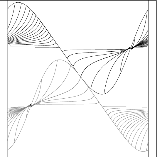
Figure 4.1 shows $\Psi(\Sigma_{1}-E_{0})$ in black and $\Psi(\Sigma_{2}-E_{0})$ in grey for the parameter $\underline{s}$ . All the black curves terminate on the tiny grey arc $\Psi(Q_{21})$ and all the grey curves terminate on the tiny black arc $\Psi(Q_{12})$ . The Technical Lemma III says that the tiny grey arc lies above the grey curve $\Psi(C_{2})$ . This is obvious from the picture.

Figure 4.2 shows the same picture for $s=1$ . Even though the parameter value $s=1$ is outside the interval of interest to us, we include the picture because the main features are more dramatic. Notice that the Technical Lemma III remains true even at this parameter. (However, our proof breaks down.)

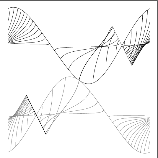
Recall that $\Sigma_{1}=\Sigma_{10}\cup\Sigma_{12}$ . The $R$ –arcs foliating $\Sigma_{10}$ are mapped to individual points on $\Psi(C_{1})$ . The $R$ –arcs foliating $\Sigma_{12}$ are mapped to black curves connecting $\Psi(C_{1})$ to the black arc $\Psi(Q_{21})$ . Here, in general

Q_{ij}=Q_{i}\cap\Sigma_{ji};\hskip 30.0pti\not=j.

(32)

The point here is that the $R$ –arcs foliating $\Sigma(E_{2},Q_{2};C_{1})$ start on $C_{1}$ and end on a subset of $Q_{2}$ . The point $\Psi(p_{0})$ is the point of tangency between the black curve $\psi(C_{1})$ and the grey curve $\psi(C_{2})$ .

Remark\quaUsing our applet, the reader can see the picture at any parameter, and can recolor each individual object, so as to see in a more direct way what part of the picture corresponds to what object.

We are going to draw two conclusions from the pictures. The main thrust of our proof is verifying that the pictures have the claimed property.

Contractible Intersections\quaFigures 4.1 and 4.2 indicate that $\Psi(\Sigma_{1}-E_{0})$ and $\Psi(\Sigma_{2}-E_{0})$ only intersect in a single point at the parameters $s=\underline{s}$ and $s=1$ respectively. Hence $A=(\Sigma_{1}-E_{0})\cap(\Sigma_{2}-E_{0})$ is a single arc. Note that $\Sigma_{j}\cap E_{0}$ is a connected arc $Q_{j}^{*}\subset Q_{j}$ . The intersection $A^{*}=Q_{1}^{*}\cap Q_{2}^{*}$ is another arc, which intersects $A$ in a single point. Hence $\Sigma_{1}\cap\Sigma_{2}=A\cup A^{*}$ , the union of two arcs arranged in a $T$ pattern—a contractible set.

Embedded Spheres\quaFigures 4.1 and 4.2 also suggest that $\Sigma_{1}$ and $\Sigma_{2}$ are embedded. We work this out here. First, we have $\Psi(\Sigma_{10}-E_{0})\subset\Psi(C_{1})$ whereas the nontrivial arcs of $\Psi(\Sigma_{12}-E_{0})$ only intersects $\Psi(C_{1})$ at one point. Therefore

\Sigma_{10}\cap\Sigma_{12}\subset C_{1}\cup E_{0}.

(33)

By symmetry

\Sigma_{10}\cap\Sigma_{12}\subset C_{1}\cup E_{2}.

(34)

Lemma 4.5 below shows that $E_{0}\cap E_{2}=\emptyset$ . Hence $\Sigma_{10}\cap\Sigma_{12}=C_{1}$ . We already know that each hemisphere $\Sigma_{1j}$ is an embedded disk, and we’ve just seen that these hemispheres just intersect along the equator. Hence $\Sigma_{1}$ is an embedded sphere. The same result holds for $\Sigma_{2}$ by symmetry.

Conclusions\quaIf the pictures are right—namely if $\Psi(\Sigma_{1}-E_{0})\cap\Psi(\Sigma_{2}-E_{0})$ is a single point—then $\Sigma_{0},\Sigma_{1},\Sigma_{2}$ are embedded spheres which have pairwise contractible intersections. But then these spheres bound balls $B_{0},B_{1},B_{2}$ with pairwise disjoint interiors. Moreover $I_{j}$ interchanges the two components of $S^{3}-\Sigma_{j}$ . This picture, at the parameter $s$ , easily implies that $\rho_{s}$ is a discrete embedding. So, to prove the Goldman–Parker conjecture, we just need to show that $\Psi(\Sigma_{1}-E_{0})\cap\Psi(\Sigma_{2}-E_{0})$ is a single point for each $s\in[\underline{s},\overline{s})$ .

4.2 Containing the image

We define $S_{12A}$ to be the region of $\mbox{\boldmath{$R$}}/2\pi\mbox{\boldmath{$Z$}}\times\mbox{\boldmath{$R$}}$ bounded by $\Psi(C_{1})$ , $\Psi(Q_{21})$ and the horizontal line through the highest point of $\Psi(Q_{21})$ , as shown in Figure 4.3.

From Technical Lemma III, the horizontal edge through the lowest point of $\Psi(Q_{21})$ is disjoint from $\Psi(C_{2})$ . We define $S_{12B}$ to be the region of $\mbox{\boldmath{$R$}}/2\pi\mbox{\boldmath{$Z$}}\times\mbox{\boldmath{$R$}}$ bounded by $\Psi(C_{1})$ , $\Psi(Q_{21})$ and the horizontal line through the lowest point of $\Psi(Q_{21})$ .

We define $S_{21A}$ and $S_{21B}$ , similarly, switching the roles of the indices $1$ and $2$ .

The $R$ –axis $R_{1}$ divides $\Sigma(E_{2},Q_{2};C_{1})$ into two halves, which we denote by $\Sigma_{12A}$ and $\Sigma_{12B}$ . Figure 4.4 shows schematically how $\Psi(\Sigma_{12A})$ sits inside $S_{12A}$ . Compare Figure 4.2. Given Technical Lemma III, the Goldman–Parker Conjecture comes down to proving the following two items, which we establish in turn.

•

Let $\alpha=\Psi(\gamma)$ , where $\gamma$ is an $R$ –arc of $\Sigma_{12A}$ . Then $\alpha$ does not intersect $\partial S_{12A}$ at an interior point.
•

$\Psi(C_{1})$ and $\Psi(C_{2})$ intersect in one point

Item 1 implies that $\Psi(\Sigma_{12A})\subset S_{12A}$ and also that $\Sigma_{12A}\cap\Sigma_{10}\subset C_{1}$ . The same holds for $\Sigma_{12B}$ and hence $\Sigma_{12}\cap\Sigma_{10}=C_{1}$ . Hence $\Sigma_{1}$ is embedded. Item 2 combines with Item 1 and with the Technical Lemma III to show that $\Psi(\Sigma_{1})\cap\Psi(\Sigma_{2})$ is a single point.

Our proof of the Goldman–Parker Conjecture boils down to establishing Items 1 and 2.

4.3 The height property

Figure 4.4 shows an enlargement of part of Figure 4.3. As in Figure 4.4 we have distinguished $5$ points on $\partial S_{12A}$ : The $2$ black points are $\Psi(R_{1}-E_{1})$ , where $R_{1}$ is the $R$ –axis of $\Sigma_{1}$ . The $2$ white points are the points of maximum and minimum height on $\Psi(C_{1})$ . The grey point is the point of $\Psi(\Sigma_{12A})$ which lies on the same horizontal line as the top white point.

Lemma 4.4.

Two arcs of $\Psi(\Sigma_{12A})$ , which start at the same horizontal level on $\Psi(C_{1})$ , end at the same point of $\Psi(Q_{21})$ . In particular, there is an arc of $\Psi(\Sigma_{12A})$ which connects the bottom white point to the grey point.

Proof.

The second statement follows as a limiting case of the first statement, so we will concentrate on the first statement. Let $\alpha_{1}$ and $\alpha_{2}$ be two $R$ –arcs of $\Sigma_{12A}$ . Let $a_{j}=\Psi(\alpha_{j})$ and let $\beta_{j}=I_{1}(\alpha_{j})$ .

1.

$a_{1}$ and $a_{2}$ have endpoints at the same horizontal level of $\Psi(C_{1})$ .
2.

Hence $\alpha_{1}\cap C_{1}$ and $\alpha_{2}\cap C_{1}$ lie in the same spinal sphere of the cospinal foliation $S(E_{0},Q_{0})$ .
3.

Hence $\beta_{1}\cap C_{1}$ and $\beta_{2}\cap C_{1}$ lie in the same spinal sphere of the cospinal foliation $S(E_{0},Q_{0})$ .
4.

Hence $\beta_{1}$ and $\beta_{2}$ lie in the same spinal sphere of the cospinal foliation $S(E_{0},Q_{0})$ .
5.

Hence $\beta_{1}\cap Q_{0}=\beta_{2}\cap Q_{0}$ .
6.

Hence $\alpha_{1}\cap Q_{2}=\alpha_{2}\cap Q_{2}$ .
7.

Hence $\Psi(\alpha_{1}\cap Q_{2})=\Psi(\alpha_{2}\cap Q_{2})$ .
8.

Hence $a_{1}$ and $a_{2}$ contain the same point of $\Psi(Q_{2})$ .

This is what we wanted to prove. ∎

Lemma 4.4 is borne out in Figures 4.1 and 4.2 and can be seen in more detail on our applet.

4.4 The interlacing property

Here we recall Figure 3.4 for convenience. Recall that $\Sigma_{1}$ is interlaced if the picture looks like the right hand side of Figure 3.4. That is, a vertical line separates the minimum of $\Psi(E_{2})$ from the minimum of $\Psi(C_{1})$ . In this section we prove that $\Sigma_{1}$ is an interlaced $R$ –sphere for all $s\in[\underline{s},\overline{s})$ . This result lets us use all the machinery from Section 3.

Lemma 4.5.

The pairs $(C_{1},E_{0})$ and $(E_{0},E_{2})$ are each generically linked.

Proof.

We already know that $(E_{0},C_{1})$ are linked. Lemma 3.13 now says that $(E_{0},E_{2})$ are linked. We just need the genericity condition. If $C_{1}$ and $E_{0}$ bound perpendicular $C$ –slices then $I_{1}$ stabilizes $E_{0}$ . By symmetry $I_{2}$ stabilizes $E_{0}$ . But then $I_{1}I_{2}$ stabilizes a $C$ –slice. This does not happen. If $E_{0}$ and $E_{2}$ bound perpendicular $C$ –slices then $E_{0}$ and $E_{1}$ bound perpendicular slices, by symmetry. But then the slices bounded by $E_{1}$ and $E_{2}$ are disjoint. Hence $E_{1}$ and $E_{2}$ are unlinked. This is a contradiction. ∎

Comparing Figure 3.4 with Figure 4.5 we see that $\Sigma_{1}$ is interlaced for the parameter $\underline{s}$ . By continuity, and Lemma 4.5, we get that $\Sigma_{1}$ is interlaced for all $s\in[\underline{s},\overline{s})$ . Lemma 4.5 prevents the picture from switching from the right hand side of Figure 3.4 to the left hand side of Figure 3.4 as $s$ varies.

4.5 No interior cusps

Let $\gamma$ be an $R$ –arc of $\Sigma(E_{2},Q_{2};C_{1})$ and let $\widehat{\gamma}$ be the $R$ –circle which contains $\gamma$ . By definition, $\widehat{\gamma}$ is an affiliate of $\Sigma(E_{2},Q_{2};C_{1})$ . Figure 4.5 shows a particular example at the parameter $\underline{s}$ . Here $\Psi(\gamma)$ in black the rest of $\Psi(\widehat{\gamma})$ in grey. The loop $\Psi(C_{1})$ is drawn in black and the loop $\Psi(E_{2})$ is drawn in grey. The vertical direction in Figure 4.5 is scaled differently than the vertical direction in Figure 4.1, because otherwise $\Psi(E_{2})$ would be quite a tall curve. (On my applet one can use many more colors.)

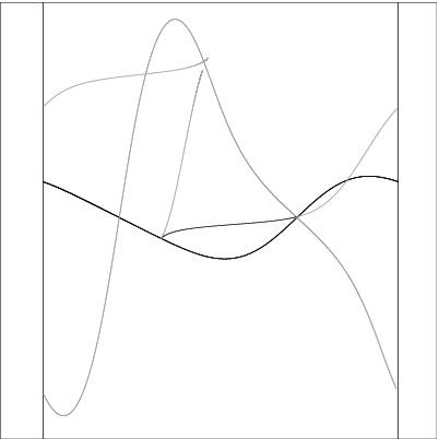
In general, let $s\in[\underline{s},\overline{s})$ . Suppose, for this parameter, that $\gamma$ is an $R$ –arc of $\Sigma(E_{2},Q_{2};C_{1})$ , not contained in the $R$ –axis of $\Sigma_{1}$ . Let $\widehat{\gamma}$ be the $R$ –circle which contains $\gamma$ . Let $\widehat{\alpha}=\Psi(\widehat{\gamma})$ and let $\alpha=\Psi(\gamma)$ . Let $\alpha_{0}=\Psi(\gamma\cap C_{1})$ .

Lemma 4.6.

$\alpha_{0}$ is a cusp of $\widehat{\alpha}$ .

Proof.

Let $\theta\in C_{1}$ be the endpoint of $\gamma$ . Let $C_{\theta}$ be the contact plane at $\theta$ . Then $I_{1}$ rotates $C_{\theta}$ by $180$ degrees. This means that $\gamma_{\theta}$ and $I_{1}(\gamma_{\theta})$ are tangent at $\theta$ . But $I_{1}(\gamma_{\theta})=\Sigma(E_{0},q_{0};\theta)$ is a fiber of $\Psi$ . Hence $\gamma_{\theta}$ is tangent to a fiber of $\Psi$ at $\theta$ . Hence $\alpha_{0}=\Psi(\theta)$ is a cusp. ∎

Lemma 4.7.

$\alpha$ has does not contain the second cusp of $\widehat{\alpha}$ .

Proof.

Write $\alpha=\Psi(\gamma)$ and let $\widehat{\gamma}$ be the $R$ –circle containing $\gamma$ . Figure 4.5 shows an example where $\alpha$ does not contain the second cusp. If there are examples where $\alpha$ does contain the second cusp then there is an example where the two endpoints of $\alpha$ are both cusps. But then this second cusp is the point of maximum height of $\alpha$ . Note that $\widehat{\gamma}$ intersects $E_{2}$ in two points. For the example under consideration, we therefore have

{\rm height\/}(\Psi(\widehat{\gamma}\cap Q_{2}))>{\rm height\/}(\Psi(\widehat{\gamma}\cap(E_{2}-Q_{2}))).

However, for the example in Figure 4.5

{\rm height\/}(\Psi(\widehat{\gamma}\cap Q_{2}))<{\rm height\/}(\Psi(\widehat{\gamma}\cap(E_{2}-Q_{2}))).

But then, by continuity, we have an example where:

{\rm height\/}(\Psi(\widehat{\gamma}\cap Q_{2}))={\rm height\/}(\Psi(\widehat{\gamma}\cap(E_{2}-Q_{2}))).

However $\gamma\cap Q_{2}$ and $\gamma\cap(E_{2}-Q_{2})$ are in harmonic position with respect to $Q_{2}$ . Thus by Lemma 3.16, $\Sigma_{1}$ is symmetric. However, Technical Lemma II and Lemma 3.18 combine to say that $\Sigma_{1}$ is asymmetric. This is a contradiction. ∎

Corollary 4.8 (Rising Property).

Let $\gamma$ be an $R$ –arc of $\Sigma(E_{2},Q_{2};C_{1})$ . If $\gamma$ is not contained in the axis then $\alpha=\Psi(\gamma)$ is nonsingular on its interior and has nowhere vanishing slope.

Proof.

This follows immediately from Lemma 3.4 and Lemma 3.5, combined with the fact that $\alpha$ has no cusps in its interior. ∎

4.6 Proof of Item 1

At the end of subsection 4.2 we reduced the whole Goldman–Parker Conjecture to the verification of two items. Here we prove the first of these items.

Let $\gamma$ be an $R$ –arc of $\Sigma_{12A}$ . Let $\alpha=\Psi(\gamma)$ . We want to show that $\alpha$ does not intersect $S_{12A}$ at an interior point. We break $\partial S_{12A}$ into three edges, as shown in Figure 4.4 From the Rising Property, the height of $\alpha$ attains its maximum at the endpoint of $\alpha$ which lies on $\Psi(Q_{21})$ . But the horizontal edge only intersects $\Psi(Q_{21})$ at its point of maximum height by Technical Lemma III. Hence $\alpha$ does not hit the horizontal edge. Since $\Sigma_{1}$ is remote $\alpha$ has positive slope. Hence $\alpha$ cannot hit the negative edge. We just have to worry about the positive edge.

Before we deal with the problem of hitting the positive edge, we want to divide the arcs of $\Psi(\Sigma_{12A})$ into two categories. Say that a positive arc is one whose endpoint lies on the positive edge of $\partial S_{12A}$ . Likewise define negative arcs. Say that the middle arc is the arc which contains the lowest point of $\Psi(C_{1})$ . This arc connects a white point to a grey point in Figure 4.4. Looking at Figure 4.2 we can see that two positive arcs appear never to cross each other whereas two negative arcs always cross each other.

Lemma 4.9.

Two positive arcs never cross each other at interior points.

Proof.

Looking at the ordering of the endpoints of the positive arcs, on $\Psi(C_{1})$ and $\Psi(Q_{2})$ respectively, we see that two positive arcs $\alpha_{1}$ and $\alpha_{2}$ must cross in at least one pair of oppositely oriented crossings, if they cross at all. By varying $\alpha_{2}$ away from $\alpha_{1}$ , as in Figure 4.6, we can produce a positive arc $\alpha_{3}$ which is tangent to $\alpha_{1}$ at some point $x$ . We write $\alpha_{j}=\Psi(\gamma_{j})$ . By the Slope Principle of subsection 3.3, the $R$ –arcs $\gamma_{1}$ and $\gamma_{3}$ intersect at some point of $\Psi^{-1}(x)$ . But this contradicts the fact that $\Sigma_{12}$ is an embedded disk. ∎

Corollary 4.10.

A positive edge does not intersect the positive arc of $C_{1}$ in a point which is interior to the positive edge.

Proof.

Suppose $\alpha_{0}$ is a positive arc which intersects the positive edge at a point $x_{0}\in\Psi(C_{1})$ . By Lemma 3.4 the arc $\alpha_{0}$ is transverse to $\Psi(C_{1})$ at the endpoint. Hence an initial open segment of $\alpha_{0}$ either is contained in the interior of $S_{12A}$ or is contained in the complement of $S_{12A}$ . Figure 4.7 shows the former option, which turns out to be the true option. Which option obtains is independent of the choice of $\alpha_{0}$ , and for $\alpha_{0}$ very near the middle arc, the former option obtains by the Rising Property. Hence, the former option always obtains. In summary, some initial portion of $\alpha_{0}$ is contained in the interior of $S_{12A}$ .

We can choose $x_{0}$ to be the first point where $\alpha_{0}$ crosses the positive edge. Let

\{\alpha_{t}|\ t\in[0,1]\}

denote the family of positive arcs such that the endpoint $e_{t}$ of $\alpha_{t}$ on $\Psi(C_{1})$ interpolates between the endpoint $e_{0}$ of $\alpha_{0}$ and the point $e_{1}=x_{0}$ . The arcs $\alpha_{0}$ and $\alpha_{t}$ cannot cross, by the previous result. Also, an initial open segment of $\alpha_{t}$ is contained in the interior of $S_{12A}$ . The only possibility is that $\alpha_{t}$ crosses the positive edge at some first point $x_{t}$ and, in order along $\Psi(C)$ the points come as

e_{0},e_{t},x_{t},x_{0}.

Since $\{e_{t}\}$ moves all the way from $e_{0}$ to $x_{0}$ and $e_{t}$ comes before $x_{t}$ (by the Rising Property) we must have some value $s$ for which $e_{s}=x_{s}$ , but this contradicts the fact that some initial open segment of $\alpha_{s}$ is contained in the interior of $S_{12A}$ .

Lemma 4.11.

Suppose that $\alpha_{1}$ is a negative arc and $\alpha_{2}$ is a positive arc. Suppose the endpoint of $\alpha_{1}$ on $\Psi(C_{1})$ is lower than the endpoint of $\alpha_{2}$ on $\Psi(C_{2})$ . Then $\alpha_{1}$ and $\alpha_{2}$ do not intersect.

Proof.

The ordering of the endpoints for $\alpha_{1}$ and $\alpha_{2}$ is the same as in Lemma 4.9. The same argument as in Lemma 4.9 works here. ∎

Corollary 4.12.

A negative arc cannot intersect the positive edge of $C_{1}$ in a point which is interior to the negative arc.

Proof.

Suppose $\alpha_{1}$ is a negative arc which intersects the positive edge. Let $x$ be the endpoint of $\alpha_{1}$ on $\Psi(C_{1})$ . Then, from the Rising Property, $\alpha_{1}$ intersects the positive edge at a point $y$ which lies above $x$ . But then $\alpha_{1}$ must cross some positive arc $\alpha_{2}$ whose endpoint lies above $x$ and below $y$ . This contradicts the previous result. ∎

Our lemmas cover all the cases. This establishes Item 1.

4.7 Proof of Item 2

Our goal is to show that $\Psi(C_{1})$ and $\Psi(C_{2})$ intersect in a single point, for all parameters $s\in[\underline{s},\overline{s})$ . We work in ${\cal H\/}$ and normalize so that $(E_{0},Q_{0})$ is in standard position and $\rho_{0}=(\mbox{\boldmath{$R$}}\times\{0\})\cup\infty$ . Then $C_{1}$ and $C_{2}$ are swapped by the $R$ –reflection $(z,t)\to(\overline{z},-t)$ which fixes $\rho_{0}$ . To fix the scale, we arrange that $C_{1}\cap C_{2}=(1,0)$ . Both $C_{1}$ and $C_{2}$ have aspect greater than $9$ by Technical Lemma I, part 3.

Lemma 4.13.

Define $\Psi_{*}(z,t)=(\arg z,t)$ . Then $\Psi_{*}(C_{1})\cap\Psi_{*}(C_{2})=(0,0)$ , with $\Psi_{*}(C_{1})$ lying on top.

Proof.

Let $s\in[\underline{s},\overline{s})$ be some parameter. $\Psi_{*}(C_{j})$ is the graph of a function $\psi_{j}$ . Up to rotations and scaling, $\psi$ satisfies the equation in Lemma 2.4, for some $A>9$ . Hence, by Lemma 2.4, the function $\psi_{j}$ is convex on an interval of length $\pi$ and concave on the complementary interval of length $\pi$ . We have parametrized $\psi$ so that $\psi(0)=\Psi(p_{0})$ . Here $p_{0}=(1,0)=C_{1}\cap C_{2}$ .

Sub-Lemma 4.14.

$\psi^{\prime\prime}(0)>0$ for all $s\in[\underline{s},\overline{s})$ .

Proof.

We compute that $\psi_{1}^{\prime\prime}(0)>0$ at the parameter $\overline{s}$ . Suppose that $\psi_{1}^{\prime\prime}(0)=0$ for some parameter $s$ . Then $\Psi_{*}(C_{1})$ and $\Psi_{*}(C_{2})$ are tangent at their inflection point. Then, by symmetry, $\Psi_{*}(C_{1})=\Psi_{*}(C_{2})$ . Here we are using Lemma 2.4 and the fact that $A(C_{j})>9$ . Since $C_{1}$ and $C_{2}$ are generically linked, this forces $C_{1}=C_{2}$ , a contradiction. Hence $\psi^{\prime\prime}(0)>0$ for all $s\in[\underline{s},\overline{s})$ . ∎

We have $\Psi_{*}(p_{0})=(0,0)$ . By symmetry we get

\psi_{1}(0)=\psi_{2}(0);\hskip 15.0pt\psi_{1}^{\prime}(0)=\psi_{2}^{\prime}(0);\hskip 15.0pt\psi_{1}^{\prime\prime}(0)=-\psi_{2}^{\prime\prime}(0).

(35)

The sublemma says that $\psi_{1}^{\prime\prime}(0)>0$ . Hence $\psi_{2}^{\prime\prime}(0)<0$ by symmetry. To establish Item 2 it suffices to show that $\psi_{1}(t)>\psi_{2}(t)$ for $t\in(0,\pi]$ . There are values $t_{1},t_{2}\in(0,\pi)$ such that $\psi_{j}^{\prime\prime}(t_{j})=0$ . The point $(t_{j},\psi_{j}^{\prime\prime}(t_{j}))$ is one of the points of $\Psi_{*}(C_{j})\cap L_{j}$ . Here $L_{j}$ is the horizontal line through the inflection points of $\Psi_{*}(C_{j})$ . We suppose $t_{2}\leq t_{1}$ , as indicated in Figure 4.8. The other case is similiar. Then on $(0,t_{2})$ we have $\psi_{1}>\psi_{2}$ because of our initial conditions at $0$ , and the fact that $\psi_{1}^{\prime\prime}>0$ on $(0,t_{1})$ and $\psi_{2}^{\prime\prime}<0$ on $(0,t_{1})$ . For $t\in[t_{2},\pi)$ the curve $\Psi_{*}(C_{2})$ lies below $L_{2}$ , and $\Psi_{*}(C_{1})$ lies completely above $L_{2}$ by Technical Lemma III (Section 7). (The point here is that $L_{j}$ contains the point $\Psi_{*}(c_{j})$ , where $c_{j}$ is the center of $C_{j}$ .) This does it. ∎

To finish our proof we compare the loxodromic elevation map $\Psi$ with $\Psi_{*}$ . Let $A_{2}^{*}\subset C_{2}$ denote the arc such that $\Psi_{*}(A_{2}^{*})$ ranges between $0$ and $\pi/2$ in the $S^{1}$ direction on $S^{1}\times\mbox{\boldmath{$R$}}$ . See Figure 4.9. Let $\pi$ be projection into $C$ .

Lemma 4.15.

$\Psi_{*}(A_{2}^{*})$ has negative slope.

Proof.

Let $m_{2}^{*}$ denote the point on $\Psi_{*}(C_{2})$ having minimum height. We can locate $Z=\pi(\Psi_{*}^{-1}(m_{2}^{*}))$ as follows: Let $A$ be the line through $0$ which contains the point $a$ on $\pi(C_{2})$ closest to $0$ . Then $Z$ is obtained from $A$ by rotating $90$ degrees about the center of $\pi(C_{2})$ , as shown. The key observations are that $\pi(C_{2})$ lies more in the lower half plane than the upper half plane. This property is true for one parameter and cannot change as the parameter varies, because the $\pi(C_{1})$ and $\pi(C_{2})$ are symmetrically placed with respect to the real axis, and never coincide. Compare Figure 4.9. From this observation, and item 3 of Technical Lemma I (subsec 5.4) we conclude that $Z$ lies in the $(-,+)$ quadrant, as shown.

Let $A_{2}^{**}$ denote the arc of $C_{2}$ which projects to the $(+,+)$ quadrant. Since $\Psi^{-1}(m_{2}^{*})$ projects to a point in the $(-,+)$ quadrant, we conclude that $\Psi_{*}(A_{2}^{**})$ has negative slope. Hence all points of $A_{2}^{**}$ lie in the lower half-space of $\cal H$ . But then the fibers of $\Psi$ , which contain points on $A_{2}^{**}$ , project to lemniscate lobes which curve around counter-clockwise. Figure 4.9 shows one such fiber $\gamma$ . In particular, if $\gamma$ contains the endpoint of $A_{2}^{*}$ then $\pi(\gamma)$ is tangent to $V$ at $0$ . (This is the $\pi/2$ condition, which defines $A_{2}^{*}$ .) But then $\pi(\gamma)$ intersects $\pi(C_{2})$ in a point which lies to the right of $V$ . Hence $A_{2}^{*}\subset A_{2}^{**}$ . ∎

Lemma 4.16.

Suppose $x_{2}\in C_{2}$ is a point such that $\Psi(x_{2})\in\Psi(C_{1})$ . Then $x$ cannot be an interior point of $A_{2}^{*}$ .

Proof.

We will suppose this is false and derive a contradiction. Let $x_{2}=(z_{2},t_{2})$ . There is some $x_{1}=(z_{1},t_{1})\in C_{1}$ and a fiber $\gamma$ of $\Psi$ such that $x_{1},x_{2}\in\gamma$ . By the previous result $t_{2}<0$ . Hence $\pi(\gamma)$ curves around clockwise, as shown in Figure 4.10.

We trace counterclockwise around $\gamma$ as indicated by the arrow in Figure 4.10. Suppose for the moment that we encounter $x_{2}$ before we encounter $x_{1}$ , as shown in Figure 4.10. The height of $\gamma$ in $\cal H$ is monotone decreasing. Hence $t_{2}>t_{1}$ . The line $L$ through $0$ and $\pi(x_{1})$ intersects $\pi(C_{1})$ at some point between $1$ and $\pi(x_{2})$ . Let $x_{2}^{*}=(z_{2}^{*},t_{2}^{*})$ be the corresponding point on $C_{2}$ . Then $x_{2}^{*}$ lies between $(1,0)$ and $x_{2}$ . In particular $x_{2}^{*}\in A_{2}^{*}$ . Since $\Psi_{*}(A_{2}^{*})$ has negative slope, we have $t_{2}^{*}>t_{2}$ . Hence $t_{2}^{*}>t_{1}$ . But then $\Psi_{*}(x_{2}^{*})$ lies above $\Psi_{*}(x_{1})$ , on the same vertical line. This is a contradiction.

To show that $\gamma$ encounters $x_{2}$ before $x_{1}$ we first introduce some terminology. For $j=1,2$ we say that a type $j$ arc is a portion of a fiber of $\Psi$ which connects a point of $E_{0}-Q_{0}$ to $C_{j}$ . The type $j$ subarc of $\gamma$ projects to the portion of $\pi(\gamma)$ which connects $0$ to $x_{j}$ . Thus, we want to show that the type $1$ sub-arc $\gamma_{1}\subset\gamma$ contains the type $2$ sub-arc $\gamma_{2}\subset\gamma$ . We are going to make an argument based on a computer plot, but we say in advance that we only use topological features of the plot. We simply need the plot to draw the reader’s attention to the relevant details.

We use the projection map $\eta$ from subsection 3.9. Figure 4.11 shows the relevant objects at the parameter $\underline{s}$ . The picture looks similar at other parameters.

•

The large black circle is $\eta(E_{0})$ . The small black circle is $\eta(C_{1})$ . The small grey circle is $\eta(C_{2})$ . The grey geodesic has $\eta(\partial Q_{0})$ for endpoints.
•

The black geodesic, which contains $\eta(C_{1})\cap\eta(C_{2})$ , is $\eta(\rho_{0})$ . The black geodesic arcs are images of the type $1$ arcs of interest to us. $\eta(\gamma)$ must project onto the same side of $\eta(R_{1})$ as these black arcs, and of course $\eta(\gamma)$ must intersect the black circle.
•

The grey arcs are images of the type $2$ arcs of interest to us. The last grey arc, the one tangent to the grey circle, is the type $2$ subarc which contains the point $z\in C_{2}$ such that $\Psi(z)$ has minimum height on $\Psi(C_{2})$ . Thus $\eta(\gamma_{2})$ must project into the region indicated by these grey arcs.

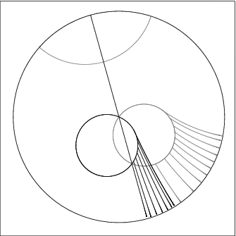
The type 1 and type 2 subarcs of $R_{0}$ coincide. As we move away from $\eta(R_{0})$ the projections of the type 1 subarcs grow longer in comparison to the corresponding projections of the type 2 subarcs. In particular $\eta(\gamma_{2})$ would be shorter than $\eta(\gamma_{1})$ . Hence $\gamma_{2}\subset\gamma_{1}$ . ∎

In summary, if $\Psi(C_{1})$ and $\Psi(C_{2})$ intersect in a second point $(x,y)$ then $x\not\in(0,\pi/2]$ . By symmetry $x\not\in[-\pi/2,0)$ . Recall that $L_{j}$ is the horizontal line in $S^{1}\times\mbox{\boldmath{$R$}}$ which contains the points of symmetry of $\Psi(C_{j})$ . Then the two points of $L_{1}\cap\Psi(C_{1})$ are $\pi$ apart. Let $s_{1}$ be this symmetry point. As we trace around $\Psi(C_{1})$ from $(0,0)$ to $s_{1}$ we remain above $\Psi(C_{2})$ . Once we reach $s_{2}$ we remain above $L_{1}$ for another $\pi$ radians of travel in the $S^{1}$ direction. It follows from Technical Lemma III that $L_{1}$ lies above every point of $\Psi(C_{2})$ . Depending on which option obtains, we have shown either that $x\not\in(0,3\pi/2]$ of $x\not\in[-3\pi/2,0)$ . Either case implies the other by symmetry. But then $x=0$ and we are done.

5 Technical Lemma I

5.1 A resume of formulas

Here we introduce the formulas which we use for our technical estimates. As a double-check, we verified all the numbered equations computationally, for the parameter $\overline{s}$ . We will usually suppress the parameter $s$ from our notation. One should view this section as a continuation of subsection 2.5. First, some quantities from subsection 2.5:

\beta=\frac{s+i}{\sqrt{2+2s^{2}}};\hskip 30.0ptA_{1}=\frac{s+17i}{s+i};\hskip 30.0ptA_{2}=\frac{12\sqrt{2}i}{\sqrt{1+s^{2}}}.

(36)

One verifies easily that

\overline{\beta}=\frac{3}{4}\times\frac{A_{1}-1}{A_{2}}.

(37)

The matrix $g_{0}=I_{1}I_{0}I_{2}$ has a positive eigenvector $(e,\overline{e},1)$ . The quantity $e$ (not to be confused with the base of the natural log) figures heavily in our estimates. As suggested by the referee, we introduce the quantity:

x=\frac{e^{2}+|e|^{2}+\overline{e}^{2}}{1-|e|^{2}}.

(38)

Here are $4$ equations, all due to the referee:

|e|^{2}=\frac{x^{2}}{9(x-1)}

(39)

|e-\overline{e}|^{2}=\frac{x(x-3)^{2}}{9(x-1)}

(40)

|2\overline{\beta}e-1|^{2}=\frac{(x-3)^{2}}{18(x-1)}

(41)

\frac{288}{1+s^{2}}=|A_{2}|^{2}=\frac{9(x-1)(x-3)^{2}}{x}

(42)

We will give the derivations below.

Note that $x>1$ by Equation 39. It follows readily from Equation 42 that

s\in[\underline{s},\overline{s}]\hskip 30.0pt\Longrightarrow\hskip 30.0ptx\in[4,\frac{817}{200}].

(43)

Recall that $\rho_{0}$ is the $R$ –circle $\{(z,\overline{z})\}\subset S^{3}$ . Recall also that $E_{0}$ is the $C$ –circle stabilized by the element $g_{0}$ . We have $E_{0}\cap\rho_{0}=\{q_{0},q_{0}^{\prime}\}$ where

q_{0}=\left[\matrix{a\cr\overline{a}}\right];\hskip 15.0ptq^{\prime}_{0}=\left[\matrix{b\cr\overline{b}}\right];\hskip 30.0pta=\frac{1+i\sqrt{2|e|^{2}-1}}{2\overline{e}}\hskip 15.0ptb=\frac{1-i\sqrt{2|e|^{2}-1}}{2\overline{e}}.

(44)

This last equation follows from the fact that

|a|^{2}=|b|^{2}=1/2;\hskip 30.0pt\langle(a,\overline{a},1),(e,\overline{e},1)\rangle=\langle(b,\overline{b},1),(e,\overline{e},1)\rangle=0.

The endpoints of the arc $Q_{0}\subset E_{0}$ are given by

\partial_{1}Q_{0}=(c,d);\qquad\partial_{2}Q_{0}=(\overline{d},\overline{c}).

We label so that $|c|^{2}\geq 1/2$ and $|d|^{2}\leq 1/2$ . We have

|c|^{2}|d|^{2}=\frac{1}{x(x-3)^{2}};\hskip 30.0pt|c|^{2}+|d|^{2}=1.

(45)

We will give the derivation below.

It follows readily from Equation 39 that:

{\rm Re\/}(a\overline{b})=\frac{-9+9x-x^{2}}{2x^{2}}

(46)

Below we will derive:

{\rm Re\/}(a\overline{\beta})=\frac{3(x-1)(9+x)-(x-3)\sqrt{(x-3)(2x-3)(9-x)}}{16x^{2}}

(47)

A similar derivation, which we omit, shows that:

{\rm Re\/}(\beta\overline{b})=\frac{3(x-1)(9+x)+(x-3)\sqrt{(x-3)(2x-3)(9-x)}}{16x^{2}}

(48)

Finally:

{\rm Im\/}(a\overline{b}+b\overline{\beta}+\beta\overline{a})=\frac{(x-3)\sqrt{(x-3)(2x-3)(x-1)}}{8x^{2}}

(49)

I’m proud to say that I found these last $3$ equations myself, though of course the referee had a much better derivation for the last one, which he communicated to me in his final comments on the paper.

5.2 The derivations

The first $4$ derivations, as well as the last one, are essentially due to the referee. We begin with a technical lemma:

Lemma 5.1.

A_{1}=\frac{e^{2}-\overline{e}^{4}}{|e|^{2}-|e|^{4}}\hskip 30.0ptA_{2}=\frac{e^{3}-\overline{e}^{3}}{|e|^{2}-|e|^{4}}\hskip 30.0pt\frac{A_{1}-1}{A_{2}}=\frac{e}{x}+\overline{e}

(50)

Proof.

The vector $\widehat{E}_{0}$ is an eigenvalue for the matrix $g_{0}$ from Equation 19. That is:

\left[\matrix{0&-1&0\cr-A_{1}&0&A_{2}\cr-A_{2}&0&-\overline{A}_{1}}\right]\left[\matrix{e\cr\overline{e}\cr 1}\right]=\lambda\left[\matrix{e\cr\overline{e}\cr 1}\right]

Reading across the top row we see that $\lambda=-\overline{e}/e$ . Reading across the second and third rows, using the relation $\overline{A}_{2}=-A_{2}$ , multiplying through by powers of $e$ , and conjugating when necessary, we get:

-A_{1}e^{2}+A_{2}e=-\overline{e}^{2}\hskip 30.0pt-A_{1}\overline{e}+A_{2}\overline{e}^{2}=-e

The first two equations in Equation 50 are now derived by the usual method of elimination. The third equation is verified by expanding out both sides, using the definition of $x$ , and the identity $e^{3}-\overline{e}^{3}=(e-\overline{e})(e^{2}+|e|^{2}+\overline{e}^{2})$ . ∎

5.2.1 Derivation of equation 39

Inspecting Equation 36, we get the equation $9|A_{1}-1|^{2}=8|A_{2}|^{2}$ . Therefore:

9|e^{2}-\overline{e}^{4}-|e|^{2}-|e|^{4}|^{2}=8|e^{3}-e^{3}|^{2}=8|e-\overline{e}|^{2}\ |e^{2}+|e|^{2}+\overline{e}^{2}|^{2}

(51)

The left hand side equals

9|e-\overline{e}|^{2}|e(1-|e|^{2})+\overline{e}(e^{2}+|e|^{2}+\overline{e}^{2})^{2}.

Therefore

9|e(1-|e|^{2})+\overline{e}(e^{2}+|e|^{2}+\overline{e}^{2})|^{2}=8|e^{2}+|e|^{2}+\overline{e}^{2}|^{2}.

Dividing through by $(1-|e|^{2})^{2}$ and cancelling the term $|e-\overline{e}|^{2}$ which occurs on both sides of Equation 51, we get $9|e+\overline{e}x|^{2}=8x^{2}$ . Expanding:

9(|e|^{2}+|e|^{2}x^{2}+e^{2}x+\overline{e}^{2}x)=8x^{2}.

The left hand side can be re-written as

9(|e|^{2}+|e|^{2}x^{2}-|e|^{2}x+x(e^{2}+|e|^{2}+\overline{e}^{2}))=9|e|^{2}(1+x^{2}-x)+x^{2}(1-|e|^{2}).

Therefore

9|e|^{2}(1+x^{2}-x))+9x^{2}(1-|e|^{2})=8x^{2}.

Solving this last equation for $|e|^{2}$ yields Equation 39.

5.2.2 Derivation of equation 40

|e-\overline{e}|^{2}=(e-\overline{e})(\overline{e}-e)=-e^{2}-\overline{e}^{2}+2|e|^{2}=-(e^{2}+|e|^{2}+\overline{e}^{2})+3|e^{2}|=

-x(1-|e|^{2})+\frac{x^{2}}{3(x-1)}=-x(1-\frac{x^{2}}{9(x-1)})+\frac{x^{2}}{3(x-1)}.

The last equation is equivalent to the right hand side of Equation 40.

5.2.3 Derivation of equation 41

From Equation 37 and the third part of Equation 50 we get

2\overline{\beta}e=\frac{3}{2x}\times(e^{2}+x|e|^{2}).

Substituting in Equation 39 and grouping terms we get

\frac{2x}{3}\times(2\overline{\beta}e-1)=e^{2}+P;\hskip 30.0ptP=\frac{6x-6x^{2}+x^{3}}{9x-9}.

(52)

Therefore

\frac{4x^{2}}{9}\times|2\overline{\beta}e-1|^{2}=|e|^{4}+(e^{2}+\overline{e}^{2})P+P^{2}=

|e|^{4}+(e^{2}+|e|^{2}+\overline{e}^{2})P+P^{2}-P|e|^{2}=|e|^{4}+x(1-|e|^{2})P+P^{2}-P|e|^{2}.

(53)

When we simplify Equation 53, using Equation 39, we get Equation 41.

5.2.4 Derivation of equation 42

The second equality in Equation 42 is the nontrivial one. From Equation 50 we get

A_{2}=(e-\overline{e})\frac{x}{|e|^{2}(1-|e|^{2})};\hskip 50.0pt|A_{2}|^{2}=\frac{x^{2}|e-\overline{e}|^{2}}{|e|^{2}(1-|e|^{2})}.

Now we plug in our equations for $|e-\overline{e}|^{2}$ and $|e|^{2}$ and simplify.

5.2.5 Derivation of equation 45

The values $c,\overline{d},e$ are all roots of

z^{3}+\left[\frac{2\overline{A}_{1}}{A_{2}}\right]z^{2}+\left[\frac{\overline{A}_{1}^{2}}{A_{2}^{2}}-\frac{A_{1}}{A_{2}^{2}}\right]z+\frac{1}{A_{2}}

This polynomial comes from solving the system of equations entailed by the equation $g_{0}(c,d,1)=\lambda(c,d,1)$ . The last term is the product of the roots. Hence

|c|^{2}|d|^{2}=\frac{1}{|A_{2}|^{2}|e|^{2}}=\frac{1}{x(x-3)^{2}}.

Since $(c,d,1)$ is a null vector we also have $|c|^{2}+|d|^{2}=1$ .

5.2.6 Derivation of equation 47

We will be a bit sketchy here, to avoid a huge mess which is best done symbolically. Note that

a\overline{\beta}=\frac{(2a\overline{e})(2\overline{\beta}e)}{4|e|^{2}}=\frac{(1+i\sqrt{2|e|^{2}-1})(\frac{3}{2x}\times(e^{2}+P)+1)}{4|e|^{2}}.

(54)

Here $P$ is as above. The only term on the right hand side of Equation 54 which is not readily expressible in terms of $x$ is the $e^{2}$ term. However, when we take twice the real part of the right hand side of Equation 54, which amounts to adding this formula to the conjugate of itself, the only terms not expressed in terms of $x$ are the real and imaginary parts of $e^{2}$ . We have

2{\rm Re\/}(e^{2})=e^{2}+\overline{e}^{2}=x(1-|e|^{2})-|e|^{2};\hskip 30.0pt({\rm Re\/}(e^{2}))^{2}+({\rm Im\/}(e^{2}))^{2}=(|e|^{2})^{2}.

(55)

Using these equations and Equation 39 we get expressions for the real and imaginary parts of $e^{2}$ in terms of $x$ . When we simplify the massive expression we arrive at Equation 47.

5.2.7 Derivation of equation 49

Noting that $a\overline{e}=e\overline{b}$ we can write:

a\overline{b}+b\overline{\beta}+\beta\overline{a}=\frac{(2a\overline{e})^{2}+2\overline{a}e(2\beta\overline{e}+2\overline{\beta}e)}{4|e|^{2}}

Using Equations 44 and 52, 55 we find that this last expression equals:

\frac{(1+i\sqrt{2|e|^{2}-1})^{2}+\frac{3}{2}(1-i\sqrt{2|e|^{2}-1})(1+|e|^{2}-|e|^{2}/x)}{4|e|^{2}}

Using Equation 39 and expanding, we get Equation 49.

5.3 Items 1 and 2

We turn now to the proof of the Technical Lemma I. Here $A$ denotes the aspect of $C_{1}$ relative to $E_{0}$ . A polar vector to a $C$ –circle $C$ is a vector $X$ such that $\langle X,\widehat{y}\rangle=0$ whenever $\widehat{y}$ is a lift of a point on $C$ . The polar vector for $C$ is unique up to scale.

Lemma 5.2.

Let $\widehat{E}_{0}$ and $\widehat{C}_{1}$ be polar vectors to $E_{0}$ and $C_{1}$ respectively. Let $A$ be the aspect of $C_{0}$ when $E_{1}$ is normalized as above. Then:

A=\frac{|\langle\widehat{E}_{0},\widehat{E}_{0}\rangle||\langle\widehat{C}_{1},\widehat{C}_{1}\rangle|}{|\langle\widehat{C}_{1},\widehat{E}_{0}\rangle|^{2}}

(56)

Moreover, the two $C$ –circles are linked provided that $A>1$ .

Proof.

The statement about the linking comes straight from [4, subsection 3.3.2]. Now for the second statement: If $E_{0}$ and $C_{1}$ are normalized as in Lemma 4.1 then the polar vectors to $E_{0}$ and $C_{1}$ , in the Siegel model, are:

\widehat{E}_{0}=\left[\matrix{0\cr 1\cr 0}\right]\hskip 30.0pt\widehat{C}_{1}=\left[\matrix{r^{2}-d^{2}\cr\sqrt{2}du\cr 1}\right]

(57)

Here $u$ is a unit complex number which is a real multiple of the projection of the center of $C_{1}$ to $C$ . For $E_{0}$ this is obvious and for $C_{1}$ it is proved by showing that any two distinct points on $C_{1}$ are $\langle,\rangle^{\prime}$ orthogonal to $\widehat{C}_{1}$ . From here an easy computation shows that the left hand side of Equation 56, computed with the Siegel Hermitian form, yields $r^{2}/d^{2}=A$ . ∎

In the ball model we have

\widehat{E}_{0}=(e,\overline{e},1);\hskip 30.0pt\widehat{C}_{1}=(0,2\overline{\beta},1).

(58)

In fact $\widehat{E}_{0}$ is the positive eigenvector for $g_{0}$ and the eigenvalue is $-\overline{e}/e$ . From Lemma 5.2 and Equations 39 and 41 we have

A=\frac{2|e|^{2}-1}{|2\overline{\beta}e-1|^{2}}=\frac{2(2x-3)}{x-3}.

(59)

For $x$ as in Equation 43 we compute that $A\in[9.5,10]$ . This establishes Items 1 and 2 of the Technical Lemma I.

5.4 Item 3

Here, as in Section 2,

C_{1}\cap C_{2}=p_{0}=(\beta,\overline{\beta},1).

Let $q_{0}$ and $q_{0}^{\prime}$ be as in subsection 5.1. Let $\mbox{\boldmath{$B$}}\co S^{3}\to\cal H$ be the Heisenberg stereographic projection which normalizes as in item 3 of Technical Lemma I (subsec 5.4). Recall that $\pi(z,t)=z$ .

Lemma 5.3.

Let $q_{0}^{\prime\prime}=(-a,-\overline{a})$ . Then $\pi\circ\mbox{\boldmath{$B$}}(q_{0}^{\prime\prime})$ is the second intersection point of $\pi(C_{1})\cap\pi(C_{2})$ .

Proof.

Let $V$ denote the $C$ –circle such that $\mbox{\boldmath{$B$}}(V)$ is vertical and $\pi(\mbox{\boldmath{$B$}}(v))$ is the second intersection point of $\pi(C_{1})\cap\pi(C_{2})$ . By symmetry $V$ lies on the Clifford torus and is stabilized by the map $(z,w)\to(\overline{w},\overline{z})$ . Also $V$ contains $(a,\overline{a})$ . Hence $V$ also contains $q_{0}^{\prime\prime}$ . ∎

We introduce the cross ratio

\chi(z_{1},z_{2},z_{3},z_{4})=\frac{(z_{1}-z_{3})(z_{2}-z_{4})}{(z_{1}-z_{2})(z_{3}-z_{4})}.

(60)

Let $\zeta\in(-\infty,0)$ . Note that $\chi(\infty,\zeta,0,1)>2$ iff $\zeta<-1$ . Note also that the restriction of $\Psi_{*}$ to $\rho_{0}$ is a Mobius transformation. Hence $\zeta=\Psi_{*}(-a,-\overline{a})$ is closer $0=\Psi_{*}(b,\overline{b})$ than is $1=\Psi_{*}(\beta,\overline{\beta})$ iff

f(s):=\chi(a,-a,b,\beta)=\frac{(a-b)(-\beta-a)}{2a(b-\beta)}>2.

(61)

Equivalently (since $|a|^{2}=|b|^{2}=|\beta|^{2}=1/2$ ) it suffices to show that

\frac{|a-b|^{2}|\beta+a|^{2}}{|\beta-b|^{2}}=\frac{(1-2\ {\rm Re\/}(a\overline{b}))(1+2\ {\rm Re\/}(a\overline{\beta}))}{1-2\ {\rm Re\/}(b\overline{\beta})}>8

(62)

It is an exercise in calculus to show that the the quantities ${\rm Re\/}(a\overline{b})$ and ${\rm Re\/}(a\overline{\beta})$ and ${\rm Re\/}(b\overline{\beta})$ are all monotone for $x$ as in Equation 43. To sketch the idea, let $f_{1}$ be the function from Equation 47. We compute explicitly that $f_{1}^{\prime}(4)=-1/16$ and we easily get the crude bound $|f_{1}^{\prime\prime}|<1$ on $[4,5]$ . Hence $f_{1}^{\prime}<0$ for $x$ in our range.

Computing at the endpoints of $[\underline{s},\overline{s}]$ we have:

{\rm Re(a\overline{b})\/}\in[.331,.344];\qquad{\rm Re(a\overline{\beta})\/}\in[.432,.438];\qquad{\rm Re(b\overline{\beta})\/}\in[.474,.477].

(63)

Hence

\frac{(1-2\ {\rm Re\/}(a\overline{b}))(1+2\ {\rm Re\/}(a\overline{\beta}))}{1-2\ {\rm Re\/}(b\overline{\beta})}\geq\frac{(1-2(.334))(1+2(.438))}{1-2(.474)}=11.9775.

(64)

This completes our proof.

Remark\quaAll our points in $C$ are confined to a single quadrant. Hence, the imaginary parts also vary monotonically. We compute:

{\rm Im\/}(b\overline{a})\in[-.374,-.363]\hskip 15.0pt{\rm Im\/}(a\overline{\beta})\in[.242,.252]\qquad{\rm Im\/}(\beta\overline{b})\in[.151,.171]

(65)

6 Technical Lemma II

6.1 Estimating $Q_{0}$

Recall that $E_{0}$ intersects the Clifford torus in points $(a,\overline{a})$ and $(b,\overline{b})$ , where $a$ and $b$ are as in Equation 44. The vectors $(a,\overline{a},1)$ and $(b,\overline{b},1)$ have real Hermitian inner product. Therefore the point $P_{r}$ , represented by the vector

r\left[\matrix{a\cr\overline{a}\cr 1}\right]+i\left[\matrix{b\cr\overline{b}\cr 1}\right]

(66)

lies in $E_{0}$ . The idea here is that the chosen lift of $P_{r}$ is null and lies in the span of $(a,\overline{a},1)$ and $(b,\overline{b},1)$ . As $r\to\infty$ the point $P_{r}$ converges to $(a,\overline{a})$ and $P_{0}=(b,\overline{b})$ . The fixed points of $g_{0}$ have the form $P_{r}$ and $P_{-r}$ where $r=r(s)$ . We define $r(\overline{s})=\infty$ , in keeping with the analysis just made.

Lemma 6.1.

$r(s)>3$ for all $s\in[\underline{s},\overline{s}]$ .

Proof.

Equation 45 gives us $|d|^{2}(1-|d|^{2})>.2079$ . It follows easily that

|d|^{2}>.294

(67)

when $x$ is as in Equation 43. This also holds for the smaller range $s\in[\underline{s},\overline{s}]$ .

We will suppose that there is some $s\in[\underline{s},\overline{s}]$ such that $r(s)=3$ and we will derive a contradiction. If $r(s)=3$ then we have

d=\frac{3\overline{a}+i\overline{b}}{3+i}.

Since $|3+i|^{2}=10$ we have

|3\overline{a}+i\overline{b}|^{2}>2.94

Using $|a|^{2}=|b|^{2}=1/2$ and expanding:

5+3i(a\overline{b}-\overline{a}b)=5-6\ {\rm Im\/}(a\overline{b})>2.94.

Hence

{\rm Im\/}(a\overline{b})<.343333.

(68)

This contradicts Equation 65, which says that ${\rm Im\/}(a\overline{b})>.36$ throughout $[\underline{s},\overline{s}]$ . ∎

6.2 Item 1

There exists a (unique) Heisenberg stereographic projection $B$ which maps $E_{0}$ to $(\{0\}\times\mbox{\boldmath{$R$}})\cup\infty$ , and has the following properties:

•

$\mbox{\boldmath{$B$}}(C_{1})$ is centered at a point on the positive real axis.
•

$\mbox{\boldmath{$B$}}(C_{1})$ projects to a circle in $C$ of radius $1$ .
•

The endpoints of $\mbox{\boldmath{$B$}}(Q_{0})$ are symmetrically located on $\mbox{\boldmath{$B$}}(E_{0})$ . Hence the $R$ –axis for $\Sigma_{1}$ is just the real line in $\mbox{\boldmath{$C$}}\times\{0\}$ .

The Siegel model polar vector for $\mbox{\boldmath{$B$}}(C_{1})$ is:

V_{3}=\left[\matrix{D\cr\sqrt{2}d\cr 1}\right]\hskip 30.0ptD=1-d^{2}

(69)

The Siegel model vectors representing the endpoints of $\mbox{\boldmath{$B$}}(Q_{0})$ are given by:

V_{1}=\left[\matrix{iu\cr 0\cr 1}\right]\hskip 50.0ptV_{2}\left[\matrix{-iu\cr 0\cr 1}\right]

(70)

In this section we prove the following result, which implies item 1 of the Technical Lemma II.

Lemma 6.2.

$u>4.2$ for all $s\in[\underline{s},\overline{s}]$ .

Given $3$ vectors $V_{1},V_{2},V_{3}\in\mbox{\boldmath{$C$}}^{2,1}$ we define:

\delta(V_{1},V_{2},V_{3})=\frac{|{\rm Im\/}(\tau)|}{|{\rm Re\/}(\tau)|}\hskip 30.0pt\tau=\langle V_{1},V_{2}\rangle\langle V_{2},V_{3}\rangle\langle V_{3},V_{1}\rangle

(71)

Using the form in Equation 7 we compute readily that:

\delta(V_{1},V_{2},V_{3})=\frac{|D^{2}-u^{2}|}{2Du}

(72)

$V_{1},V_{2},V_{3}$ correspond to the following vectors in the ball model:

P_{r}\hskip 30.0pt-P_{-r}\hskip 30.0pt\widehat{C}_{1}=\left[\matrix{0\cr 2\overline{\beta}\cr 1}\right]

(73)

(We prefer to use $-P_{-r}$ in place of $P_{-r}$ .) It is convenient to define:

U_{a}=\langle\left[\matrix{a\cr\overline{a}\cr 1}\right],\widehat{C}_{1}\rangle=2\overline{a}\beta-1\hskip 30.0ptU_{b}=\langle\left[\matrix{b\cr\overline{b}\cr 1}\right],\widehat{C}_{1}\rangle=2\overline{b}\beta-1\hskip 30.0pt

(74)

Then

\langle P_{r},\widehat{C}_{1}\rangle=rU_{a}+iU_{b};\quad\langle\widehat{C}_{1},-P_{-r}\rangle=r\overline{U}_{a}+i\overline{U}_{b};\quad\langle P_{r},-P_{-r}\rangle\in i\mbox{\boldmath{$R$}}.

From this we get:

\delta(V_{1},V_{2},V_{3})=\bigg|\frac{r|U_{a}|^{2}-r^{-1}|U_{b}|^{2}}{{2\rm Re\/}(U_{a}\overline{U}_{b})}\bigg|

(75)

From Equation 63 we have:

|U_{a}|^{2}=|1-2\overline{a}\beta|^{2}=2-4\ {\rm Re\/}(a\overline{\beta})>.248

|U_{a}|^{2}=|1-2\overline{b}\beta|^{2}=2-4\ {\rm Re\/}(b\overline{\beta})<.104

Using Equations 46, 47, 54 and 74 we compute that:

2{\rm Re\/}(U_{a}\overline{U}_{b})=\frac{-3(3-4x+x^{2})}{2x^{2}}<.301

for $x$ as in Equation 43. Therefore

\delta(V_{1},V_{2},V_{3})=\delta(P_{r},-P_{-r},\widehat{C}_{1})\geq\frac{3(.248)-(1/3)(.104)}{(.301)}>2.35

Combining our last result with Equation 72 we get $|-D^{2}+u^{2}|\geq 4.7Du.$ Since $u>0$ for all parameters, the quantity $-D^{2}+u^{2}$ cannot change sign. For otherwise we would have $0>Du$ . Hence $u^{2}>4.7Du$ . From Technical Lemma I we have:

D=1-\frac{1}{d^{2}}>1-\frac{1}{9.5}>.894

Hence $u>(4.7)(.894)>4.2.$ This completes our proof.

6.3 Item 2

We normalize by the map $B$ so that all our calculations take place in $\cal H$ . So, $C_{1}$ is a $C$ –circle, centered on a point $c_{1}\in\mbox{\boldmath{$R$}}^{+}$ and $C_{1}$ projects to a circle of radius $1$ . Since the aspect of $C_{1}$ is at least $9$ we conclude that $c\in(0,1/3].$ Now $I_{1}$ is a $C$ –reflection in $C_{1}$ . The $x$ –axis is precisely $R_{1}$ , the axis for $\Sigma_{1}$ . Note that $R_{1}$ intersects $C_{1}$ twice, at points which are precisely $2$ units away from each other. The restriction of $I_{1}$ to $R_{1}$ is a Mobius transformation.

Lemma 6.3.

$E_{2}=I_{1}(E_{0})$ intersects $R_{1}$ in two points. One of the points is $(c,0)$ and the other one is $(-1/c+c,0)$ .

Proof.

This follows from the fact that the restriction of $I_{1}$ to $\mbox{\boldmath{$R$}}^{1}$ is an inversion in the segment of radius $1$ centered at $0$ . ∎

Thus we see that $E_{2}$ projects to a circle diameter $1/c\geq 3.$ Moreover, the center of $E_{1}$ is $(-1/2c+c)<-7/6.$ Now $E_{1}$ is contained in the contact plane based at its center. From this we see that $E_{2}$ is contained in a contact plane of slope at least $7/3$ . (Here, and below, slope means vertical rise divided by horizontal run.) Compared to $C_{1}$ , the $C$ –circle $E_{2}$ is a big and tall set.

Lemma 6.4.

Both endpoints of $Q_{2}$ are at most $1/4$ from the horizontal plane $\mbox{\boldmath{$C$}}\times\{0\}$ .

Proof.

Working in the Siegel model, the endpoints of $Q_{0}$ have lifts $V_{1}$ and $V_{2}$ , as Equation 70 and the polar vector $V_{3}$ for $C_{1}$ is as in Equation 69. Using Equation 5 relative to the Siegel form we have

I_{C_{1}}(V_{1})=-\left[\matrix{iu\cr 0\cr 1}\right]+2\frac{iu+D}{2D-2d^{2}}\left[\matrix{D\cr\sqrt{2}d\cr 1}\right]=\left[\matrix{D^{2}+i(uD-u)\cr*\cr D-1+iu}\right].

(The starred entry is irrelevant to us.) Multiplying through by $D-1-iu$ we see that $I_{C_{1}}(V_{1})$ is a scalar multiple of the matrix

\left[\matrix{P(u,D)+iu(1-2D)\cr*\cr u^{2}+(D-1)^{2}}\right].

(76)

Here $P(u,d)$ is a real polynomial in $u$ and $D$ whose form is not important to us. If $(z,t)$ is the point represented by $I_{C_{1}}(V_{1})$ , then

|t|=\frac{u|1-2D|}{u^{2}+(D-1)^{2}}<\frac{|1-2D|}{u}\leq 1/u\leq 1/4.

But the point $(z,t)$ is one of the endpoints of $Q_{2}=I_{1}(Q_{0})$ . The same argment works for the other endpoint of $Q_{2}$ . ∎

Here are three geometric facts:

1.

$Q_{2}$ is centered at $0$ in $\cal H$ and extends upwards at most $1/4$ in either direction. Since $E_{2}$ is contained in a contact plane of slope at least $7/3$ , the circle $E_{2}$ has slope $7/3$ at the origin by symmetry. Since $Q_{2}$ rises up only $1/4$ in either direction away from the origin, we see easily that every point of $Q_{2}$ has slope greater than $1$ .
2.

Given that every point of $Q_{2}$ has slope greater than $1$ , we see that the projection $\pi(Q_{2})$ is contained in the dist $\Delta_{1/4}$ of radius $1/4$ about the origin.
3.

Any harmonic $R$ –arc which intersects $Q_{2}$ has slope less than $1/2$ at the intersection point, because this $R$ –arc is integral to the contact structure and the intersection point projects inside $\Delta_{1/4}$ .

These properties together imply that $\Psi(Q_{2})$ does not contain any extrema of the height function, even at the endpoints. This establishes Item 2 of Technical Lemma II.

Remark\quaA more intuitive way to see the same result is that $E_{2}$ is extremely tall in comparison to $Q_{2}$ , and the fibers of $\Psi$ are fairly straight near $Q_{2}$ (because they have large diameter) and hence there is no way the height of $\Psi|_{E_{2}}$ takes on its extrema on $Q_{2}$ .

7 Technical Lemma III

7.1 Estimating $Q_{21}$

We continue our work from the previous chapter. In this section, we continue to normalize using $B$ . However, our main estimate is independent of the normalization.

Recall that $\Psi$ is the loxodromic elevation map, the map of interest to us. Given a subset $X$ , which is disjoint from $E_{0}$ , let $2\|X\|$ denote the “vertical diameter” of the set $\Psi(X)$ . By this we mean that $2\|X\|$ denotes the maximum difference in heights between two points of the form $\Psi(p_{1})$ and $\Psi(p_{2})$ , where $p_{1},p_{2}\in X$ . We call $\|X\|$ the vertical $\Psi$ –radius of $X$ . This quantity is not quite canonical; it depends on us choosing a scaling factor for the image of $\Psi$ . However, we shall always be interested in quantities of the form $\|X\|/\|Y\|$ , and this ratio is independent of the way we scale $\Psi$ . The main goal of this section is to prove

Lemma 7.1.

\frac{\|Q_{12}\|}{\|C_{1}\|}<\frac{1}{15}.

(77)

for all $s\in[\underline{s},\overline{s}]$ .

So far we have estimated quantities in $\cal H$ and we need to translate the information we have gathered into terms related to $\Psi$ . Here is an outline of how we will do this. For $X\subset{\cal H\/}$ let $\|X\|^{\prime}$ denote half the width of the smallest vertical slab which contains $X$ . At the parameter $s=\overline{s}$ we have $\|X\|^{\prime}=\|X\|$ . We want to compare $\|X\|^{\prime}$ and $\|X\|$ in general. For this purpose we let $[X]\subset E_{0}-Q_{0}$ denote the set of all (lower) endpoints of harmonic $R$ –arcs which contain points of $X$ . These $R$ –arcs are meant to be harmonic with respect to $(E_{0},Q_{0})$ . They are the arcs used in the definition of $\Psi$ . Here are the estimates we will prove:

1.

$\|Q_{12}\|^{\prime}/\|C_{1}\|^{\prime}<1/17$ .
2.

$\|[Q_{12}]\|^{\prime}<\|Q_{12}\|^{\prime}$ and $\|[C_{1}]\|^{\prime}>(15/17)\|C_{1}\|^{\prime}$ .
3.

$\|Q_{12}\|/\|C_{1}\|<\|[Q_{12}]\|^{\prime}/\|[C_{1}]\|^{\prime}$ .

These estimates combine, in a straightforward way, to establish Lemma 7.1.

7.1.1 First estimate

We have $Q_{21}=I_{1}(Q_{01})$ . Here $Q_{01}\subset Q_{0}$ consists of points $x$ such that $x$ is the endpoint of an $R$ –arc which is harmonic with respect to $(E_{0},Q_{0})$ and which intersects $C_{1}$ . The endpoints of $Q_{01}$ are represented by vectors of the form:

V_{1}^{\prime}=\left[\matrix{iu^{\prime}\cr 0\cr 1}\right]\hskip 30.0ptV_{2}^{\prime}=\left[\matrix{-iu^{\prime}\cr 0\cr 1}\right]

(78)

The two endpoints $t_{1}$ and $t_{2}$ of any $R$ –arc, harmonic with respect to $(E_{0},Q_{0})$ , satisfy

t_{1}t_{2}=u^{2}>17,

and also $|t_{1}|<\|C_{1}\|^{\prime}$ . Hence $u^{\prime}>17\|C_{1}\|^{\prime}$ . The same argument as in Lemma 6.4 now shows that both endpoints of $Q_{21}$ are at most

1/(17/\|C_{1}\|^{\prime})=\|C_{1}\|^{\prime}/17

away from $\mbox{\boldmath{$C$}}\times\{0\}$ . Hence $\|Q_{12}\|^{\prime}<\|C_{1}\|^{\prime}/17$ .

7.1.2 The second estimate

Our harmonic arcs vary monotonically in height from their lower to their upper endpoints. Hence $\|[Q_{12}]\|^{\prime}\leq\|Q_{12}^{\prime}\|$ . This estimate is true for any set $X$ , actually. The other estimate is the interesting one.

Let $\eta$ be the map described in subsection 3.9. To do our analysis efficiently we post-compose $\eta$ with a Mobius transformation so that $\eta$ is the identity on $E_{0}$ and $\eta({\cal H\/})$ is the left half plane. (The HYP1 coordinate system in our applet is precisely this map.) $\eta$ conjugates the Heisenberg automorphism $(z,t)\to(rz,r^{2}t)$ to the hyperbolic isometry $z\to rz$ . Hence, the restriction of $\eta$ to the $R$ –circle $R_{1}=R\times\{0\}$ is the map $r\to r^{2}$ .

let $(c,0)$ denote the center of $C_{1}$ . Here $c\in(0,1/3]$ as in subsection 6.3. Since $C_{1}$ projects to a circle of radius $1$ we have $\|C_{1}\|^{\prime}=2c$ . Now, $C_{1}$ intersects $R_{1}$ in the two points $c-1$ and $c+1$ . Hence $\eta(C_{1})$ is the circle of radius $2c$ which intersects the positive real axis in the points $(1-c)^{2}$ and $(1+c)^{2}$ . Figure 7.1 shows the picture.

Let $\alpha$ be a harmonic arc which contains a point of $C_{1}$ . Then $\eta(\alpha)$ is a semicircle which connects two points of the $y$ –axis which are harmonic with respect to the endpoints of $Q_{0}$ . The upper endpoint of $Q_{0}$ is at least $4$ away from the origin. Also, the lower endpoint of $\eta(\alpha)$ is at most $2c$ away from $0$ . Hence the other endpoint of $\eta(\alpha)$ is at least $4^{2}/(2c)>8/c$ away from the origin. Hence $\eta(\alpha)$ has radius at least

R(c)=\frac{4}{c}-c

(79)

Note that $R(c)>11$ for $c\in[0,1/3]$ .

We want to compare the point $h_{2}$ where $\eta(\alpha)$ intersects the $y$ –axis with the point $h_{1}$ where the horizontal line $\Lambda$ tangent to $\eta(C_{1})$ intersects the $y$ –axis. These two points are shown in Figure 7.1. Our goal is to show that $h_{2}/h_{1}>15/17$ . Let $\lambda$ be the length of the portion of $\Lambda$ contained inside $\eta(C_{1})$ . This segment is drawn thickly in Figure 7.1. Using a familiar fact from high school geometry we have

(h_{1}-h_{2})(2R(c)-(h_{1}-h_{2}))\leq\lambda^{2}<(c+(1-c)^{2})^{2}.

(80)

The right hand side of the equation comes from the fact that the intersection $\Lambda\cap\eta(C_{1})$ occurs closer to the $y$ –axis than does the center of $\eta(C_{1})$ .

To simplify this equation note that $2R(c)>22$ and certainly $h_{1}-h_{2}<1$ . Hence

(2R(c)-(h_{1}-h_{2}))>\frac{21}{22}R(c).

Therefore (using the fact that $h_{1}=2c$ ) we have

1-\frac{h_{2}}{h_{1}}=\frac{h_{1}-h_{2}}{h_{1}}=\frac{h_{1}-h_{2}}{2c}<\frac{22}{21}\times\frac{(100/81)}{4cR(c)}\leq\frac{1}{12}<\frac{2}{17}.

(81)

In particular $h_{2}/h_{1}>15/17$ , as claimed. (We will use the stronger estimate in Equation 81 below.)

7.1.3 The third estimate

At this point we need to look at the loxodromic elevation map $\Psi$ geometrically. We need to quantify the difference in heights between the two points $\Psi(p_{1})$ and $\Psi(p_{2})$ . Let $\alpha_{j}$ be the harmonic arc which contains $p_{j}$ . Let $x_{j}\in E_{0}-Q_{0}$ be the relevant endpoint of $\alpha_{j}$ . Let $u_{1}=u$ and $u_{2}=-u$ be the two endpoints of $Q_{0}$ . Then, up to a constant, the difference in heights of $\Psi(p_{1})$ and $\Psi(p_{2})$ is:

\log\frac{(u_{1}-x_{2})(u_{2}-x_{1})}{(u_{1}-x_{1})(u_{2}-x_{2})}

(82)

This quantity is none other than the hyperbolic radius of the segment $[x_{1},x_{2}]$ , when the segment $[-u,u]=E_{0}-Q_{0}$ is identified with the hyperbolic line. This interpretation comes from the fact that the quantity in Equation 82 is invariant under Heisenberg automorphisms of $(E_{0},Q_{0})$ , and $\Psi$ conjugates such maps to vertical translations.

After rotating the picture sideways (so as to work with the $x$ –axis rather than the $y$ –axis) our third estimate reduces to the following situation. We have points $u$ and $-u$ as reference points. We have positive $0<v<w<u$ and we consider the intervals $I_{v}=[-v.v]$ and $I_{w}=[-w,w]$ . We let $\|I_{v}\|_{u}$ denote the hyperbolic radius of the segment $I_{v}$ when the interval $[u,-u]$ is identified with the hyperbolic line. Likewise we define $\|I_{w}\|_{u}$ .

To make our third estimate, we have in mind that

[Q_{12}]=I_{v};\hskip 50.0pt[C_{1}]=I_{w}.

\|[Q_{12}]\|^{\prime}=\|I_{v}\|_{\infty};\hskip 30.0pt\|[C_{1}]\|^{\prime}=\|I_{w}\|_{\infty};

We have

\|Q_{12}\|=\|I_{v}\|_{u};\hskip 30.0pt\|C_{1}\|=\|I_{w}\|_{u}.

Here our specific choice of $u$ is as in Equation 70. Thus, to establish our third estimate, it suffices to show that:

\frac{v}{w}>\frac{\|I_{v}\|_{u}}{\|I_{w}\|_{u}}=\frac{\log(\frac{(u+v)^{2}}{(u-v)^{2}})}{\log(\frac{(u+w)^{2}}{(u-w)^{2}})}=\frac{\log(u+v)-\log(u-v)}{\log(u+w)-\log(u-w)}

This is an easy exercise in calculus. This completes our proof of the third estimate.

7.2 Estimating the gap

At this point we have done the hardest part of the estimate, which involved controlling $\Psi(Q_{21})$ . Given Lemma 7.1 we are back to a problem involving the two curves $\Psi(C_{1})$ and $\Psi(C_{2})$ . It is difficult to draw these curves well, so we will consider $\eta(C_{1})$ and $\eta(C_{2})$ , where $\eta$ is the map considered in the previous section. Given the work done in the previous section, we will see readily how to translate back and forth between $\eta$ coordinates and $\Psi$ coordinates.

Figure 7.2 shows a schematic (and fairly accurate) picture of $\eta(C_{1})$ and $\eta(C_{2})$ . Here $\eta$ is the map we used in the previous section.

Regarding this picture:

•

The two white dots on the $y$ –axis are the endpoints of $\eta(Q_{0})$ .
•

The two black dots are the hyperbolic centers of $\eta(C_{1})$ and $\eta(C_{2})$ .
•

All the geodesics drawn are orthogonal to the geodesic joining the endpoints of $\eta(Q_{0})$ . Indeed, these geodesics are all certain images of harmonic $R$ –arcs.
•

For $j=1,2$ , we have $\gamma_{j}=\eta(R_{j})$ , where $R_{j}$ is the $R$ –axis of $C_{j}$ .
•

$\|C_{1}\|$ is the hyperbolic distance between $\gamma_{1}$ and $\gamma_{2}$ and equally well the hyperbolic distance between $\gamma_{2}$ and $\gamma_{4}$ .
•

The geodesic $\gamma_{5}$ contains the lower endpoint of $\eta(Q_{21})$ .

To finish the Technical Lemma III we just need to show that $\eta(Q_{21})$ lies above the geodesic $\gamma_{3}$ . Let $d_{ij}$ denote the hyperbolic distance between $\gamma_{i}$ and $\gamma_{j}$ . Lemma 7.1, interpreted in terms of $\eta$ , says that:

\frac{d_{14}}{d_{15}}<\frac{1}{15}

(83)

To prove item 1 of Technical Lemma III it suffices to establish the inequality:

\frac{d_{13}}{d_{14}}>\frac{1}{15}

(84)

Using a bit of algebra, we see that Equation 84 is equivalent to the more symmetric:

\frac{d_{34}}{d_{12}}<\frac{7}{8}

(85)

Remark\quaOur normalization here is slightly different than in the previous section. We are now normalizing so that reflection in the $x$ axis interchanges $\eta(C_{1})$ and $\eta(C_{2})$ . The reason we have changed normalizations is that previously we were just concentrating on $C_{1}$ and now we need to treat both $C_{1}$ and $C_{2}$ . Note that Lemma 7.1 is independent of normalization, as we mentioned above.

Let $d^{\prime}_{12}$ denote the Euclidean distance between the centers of $\eta(C_{1})$ and $\eta(C_{2})$ and let $d^{\prime}_{34}$ denote the Euclidean distance between the point of maximum height on $\eta(C_{2})$ and the point of minumum height of $\eta(C_{1})$ .

Lemma 7.2.

Equation 85 is true provided that

\frac{d^{\prime}_{34}}{d^{\prime}_{12}}<\frac{4}{5}.

(86)

Proof.

Our proof here is very much like what we did in the previous section, for Estimates 2 and 3. Estimate 3 works exactly the same way, and Estimate 3 is replaced by the statements that

d_{34}<d^{\prime}_{34};\hskip 40.0ptd_{12}>\frac{11}{12}d^{\prime}_{12}.

(87)

Thus, if Equation 86 holds then:

\frac{d_{34}}{d_{12}}<\frac{12}{11}\times\frac{4}{5}<\frac{7}{8}

The first part of Equation 87 is immediate, as above. The second part of Equation 87 is similar to what we have already done, though we have to think about our new normalization. In the old normalization we knew that $\eta(C_{1})$ was centered at the real axis, and had a center which was at most $10/9$ from the $y$ –axis. (In the old normalization $\eta(C_{2})$ was some other circle below $\eta(C_{1})$ .) Our new normalization is obtained by the old one by applying a hyperbolic isometry $I$ translating along the geodesic joining the endpoints of $\eta(Q_{0})$ . The hyperbolic isometry is chosen so that $\eta(C_{1})$ and $\eta(C_{2})$ are moved into symmetric position.

Let $h_{1}$ denote the Euclidean distance between the centers of $\eta(C_{1})$ and $\eta(C_{1})$ . Let $h_{2}$ denote the Euclidean length of the segment on the $y$ –axis between $\gamma_{1}$ and $\gamma_{2}$ . We want to show that $h_{2}/h_{1}<11/12$ . This is the same as showing that:

1-\frac{h_{2}}{h_{1}}<1/12

The argument given in subsection 7.1.2 goes through, once a few changes are noted.

By construction, the $x$ –coordinate of the hyperbolic center of the new $\eta(C_{1})$ is less than the $x$ –coordinate of the hyperbolic center of the old $\eta(C_{1})$ , which is in turn less than the $x$ coordinate of the Euclidean center of the old $\eta(C_{1})$ . We conclude that the Euclidean distance from the hyperbolic center of the new $\eta(C_{1})$ to the $y$ –axis is at most $10/9$ . (This hyperbolic center is the intersection point of $\gamma_{1}=\eta(\alpha_{1})$ and $\Lambda$ , the curves from subsection 7.1.2.) The radius of the circle containing $\gamma_{1}$ is still at least $R(c)$ . Having made these definitions, we see that the rest of the argument in subsection 7.1.2 is the same. ∎

By the previous result, Equation 86 implies item 1 of Technical Lemma III. Since $4/5<1$ , Equation 86 implies item 2 of Technical Lemma III. Thus, to finish the proof of Technical Lemma III we just have to verify Equation 86.

7.3 Back to Heisenberg space

Figure 7.3 shows the picture of $\pi(C_{1})$ and $\pi(C_{2})$ in $C$ . Referring to Figure 7.3, we will show that Technical Lemma III is true provided that $\sin(\theta)>5/9$ .

Let $c_{1}=z+it$ be the center of $C_{1}$ . The quantity $d_{12}^{\prime}$ is just the vertical distance between centers of the two circles. The quantity $d_{34}^{\prime}$ is the vertical distance between the minimum height point on $C_{1}$ and the maximum height point on $C_{2}$ .

The outer edge of the rectangle in Figure 7.3 is tangent to $\pi(C_{1})$ and parallel to axis 1, the $R$ –circle through the center of $C_{1}$ which intersects $C_{1}$ in two other points. The number $R$ is the radius of $C_{1}$ .

The vertical distance between the two centers is twice the distance from the center of $C_{1}$ to $\mbox{\boldmath{$C$}}\times\{0\}$ . This latter distance is $2|z|S$ because $S$ runs perpendicular to axis 1 and joins a point on $C_{1}$ to the point $(1,0)$ . The vertical distance between the max of $C_{2}$ and the min of $C_{1}$ is twice the vertical distance from $\mbox{\boldmath{$C$}}\times\{0\}$ to the min of $C_{1}$ . This distance is $2|z|T$ . Therefore

\frac{d^{\prime}_{34}}{d^{\prime}_{12}}=\frac{T}{S}=\frac{R-R\sin(\theta)}{R\sin(\theta)}=\frac{1}{\sin(\theta)}-1.

If $\sin(\theta)>5/9$ then the quantity on the right is less than $4/5$ .

7.4 The end of the proof

We will suppose that $\sin(\theta)<5/9$ and derive a contradiction.

7.4.1 Siegel model computation

The center of $C_{1}$ is the point $c=z+it$ . In Section 5 we saw that $C_{1}$ has aspect less than $10$ . Hence

\frac{R}{|z|}<\sqrt{10}.

(88)

In the Siegel model, the vectors representing $0,\infty,c$ are respectively:

V_{1}=\left[\matrix{0\cr 0\cr 1}\right]\hskip 30.0ptV_{1}=\left[\matrix{1\cr 0\cr 0}\right]\hskip 30.0ptV_{1}=\left[\matrix{-|z|^{2}+it\cr\sqrt{2}z\cr 1}\right]

(89)

Letting $\delta$ be the invariant from Equation 71 we have

\delta(V_{1},V_{2},V_{3})=\frac{t}{|z|^{2}}=\frac{2|z|R\sin(\theta)}{|z|^{2}}=\frac{R}{|z|}\times 2\sin(\theta)<\sqrt{10}\times\frac{10}{9}<3.52.

(90)

7.4.2 Ball model computation

In the ball model the corresponding vectors are:

U_{1}=\left[\matrix{b\cr\overline{b}\cr 1}\right]\hskip 30.0ptU_{2}=\left[\matrix{a\cr\overline{a}\cr 1}\right]\hskip 30.0ptU_{3}=\left[\matrix{-1&0&0\cr 0&3&-4\overline{\beta}\cr 0&4\beta&-3}\right]\left[\matrix{a\cr\overline{a}\cr 1}\right]

(91)

Note that $\langle U_{1},U_{2}\rangle\in\mbox{\boldmath{$R$}}$ . Also $\langle U_{2},U_{3}\rangle\in\mbox{\boldmath{$R$}}$ because these two vectors are exchanged by $I_{1}$ . Therefore $\delta(V_{1},V_{2},V_{3})=|{\rm Im\/}(\tau)|/|{\rm Re\/}(\tau)|$ , where

\tau=\langle U_{1},U_{3}\rangle=3+3(a\overline{b}+b\overline{a})-4a\overline{b}-4b\overline{\beta}-4\beta\overline{a}.

(92)

Using Equations 46, 47, 48, and 49 we get:

\delta(V_{1},V_{2},V_{3})=\sqrt{\frac{(x-1)(2x-3)}{x-3}}

(93)

A bit of calculus now shows that

\delta(V_{1},V_{2},V_{3})>3.83

(94)

in our range of parameters. This contradicts Equation 90 and we are done.

References

[1] S Anan’in, H Grossi, N Gusevskii, Complex Hyperbolic Structures on Disc Bundles over Surfaces I, preprint (2003)
[2] D B A Epstein, Complex hyperbolic geometry, from: “Analytical and geometric aspects of hyperbolic space (Coventry/Durham, 1984)”, London Math. Soc. Lecture Note Ser. 111, Cambridge Univ. Press, Cambridge (1987) 93–111 \MR903851
[3] E Falbel, J R Parker, The moduli space of the modular group in complex hyperbolic geometry, Invent. Math. 152 (2003) 57–88 \MR1965360
[4] W M Goldman, Complex hyperbolic geometry, Oxford Mathematical Monographs, The Clarendon Press Oxford University Press, New York (1999) \MR1695450
[5] W M Goldman, J R Parker, Complex hyperbolic ideal triangle groups, J. Reine Angew. Math. 425 (1992) 71–86 \MR1151314
[6] R E Schwartz, Ideal triangle groups, dented tori, and numerical analysis, Ann. of Math. (2) 153 (2001) 533–598 \MR1836282
[7] R E Schwartz, Degenerating the complex hyperbolic ideal triangle groups, Acta Math. 186 (2001) 105–154 \MR1828374
[8] R E Schwartz, Spherical CR Geometry and Dehn Surgery, preprint of Research Monograph (2004)
[9] R E Schwartz, An Interactive Proof of the G-P Conjecture, Java applet (2004) http://www.math.brown.edu/~res/Java/App45/test1.html
[10] S Wolfram, The Mathematica book, Wolfram Media, Inc. Champaign, IL (1999) \MR1721106

A better proof of the Goldman–Parker conjecture

Abstract

keywords

1 Introduction

2 Background

2.1 Complex hyperbolic geometry

2.1.1 The ball model

2.1.2 Slices

2.1.3 Isometries

2.2 Heisenberg space

2.2.1 Basic definitions

2.2.2 The contact distribution

2.3 Spinal spheres

2.3.1 Basic definitions

2.3.2 Generic tangencies with spinal spheres

Lemma 2.1.

Proof.

Corollary 2.2.

Proof.

2.4 Equations for 𝑪C–circles

Lemma 2.3.

Proof.

Lemma 2.4.

Proof.

2.5 Ideal triangle groups

2.5.1 The basic definition

2.5.2 Some associated objects

3 Loxodromic 𝑹R–spheres

3.1 The cospinal foliation

Lemma 3.1.

Proof.

Lemma 3.2.

Proof.

3.2 Loxodromic 𝑹R–cones and 𝑹R–spheres

Lemma 3.3.

Proof.

3.3 The elevation map

Lemma 3.4.

Proof.

3.4 More details on slopes

Lemma 3.5.

Proof.

Lemma 3.6.

Proof.

Corollary 3.7 (Slope Principle).

Proof.

3.5 Images of 𝑪C–circles

Lemma 3.8.

Proof.

Lemma 3.9.

Proof.

Corollary 3.10.

Proof.

3.6 Images of linked 𝑹R–circles

Lemma 3.11.

Proof.

Corollary 3.12 (Elevation Image).

Proof.

3.7 Linking of the poles

Lemma 3.13.

Proof.

3.8 The Two Cusp Lemma

Lemma 3.14 (Two Cusp).

Lemma 3.15.

Proof.

3.9 Asymmetry

Lemma 3.16 (Asymmetry Lemma).

Proof.

Lemma 3.17.

Proof.

Lemma 3.18.

Proof.

3.10 Remoteness

Lemma 3.19.

Proof.

4 The proof

4.1 Main construction

Lemma 4.1 (Technical Lemma I).

Lemma 4.2 (Technical Lemma II).

Lemma 4.3 (Technical Lemma III).

2.4 Equations for $C$ –circles

3 Loxodromic $R$ –spheres

3.2 Loxodromic $R$ –cones and $R$ –spheres

3.5 Images of $C$ –circles

3.6 Images of linked $R$ –circles

6.1 Estimating $Q_{0}$

7.1 Estimating $Q_{21}$