跳到论文正文
W Papers独立论文阅读器 arXiv:math/0508153 论文正文 计算阅读时间 · 0%
引用这篇论文根据当前论文元数据生成,正式投稿前建议核对。


License: Assumed arXiv.org perpetual non-exclusive license
arXiv:math/0508153v1 [math.CO] 08 Aug 2005

On Expected Factors in Reduced Decompositions in Type BB

Bridget Eileen Tenner Address: Department of Mathematics, Massachusetts Institute of Technology, 77 Massachusetts Ave, Cambridge, MA 02139, USA Email address: bridget@math.mit.edu
Date: August 10, 2005
Abstract.

The expected number of Yang-Baxter moves appearing in a reduced decomposition of the longest element of the Coxeter group of type BnB_{n} is computed to be 2−4/n2-4/n. For the same element, the expected number of 01010101 or 10101010 factors appearing in a reduced decomposition is 2/(n2−2)2/(n^{2}-2).

1. Introduction

Let 𝔖nB\mathfrak{S}_{n}^{B} denote the Coxeter group of type BB on {±1,…,±n}\{\pm 1,\ldots,\pm n\}, also known as the hyperoctahedral group. This is the group of signed permutations ww on {±1,…,±n}\{\pm 1,\ldots,\pm n\}, with the requirement that w⁡(−i)=−w⁡(i)w(-i)=-w(i). For ease of notation, a negative sign will be written beneath an integer, rather than before it. An element w∈𝔖nBw\in\mathfrak{S}_{n}^{B} will be written w=w(1)⋯w(n)w=w(1)\cdots w(n), where ww maps i↦w⁡(i)i\mapsto w(i) (and i¯↦w⁡(i)¯\underline{i}\mapsto\underline{w(i)}). Notice that the element ww is completely determined by the values of w⁡(1),…,w⁡(n)w(1),\ldots,w(n). The group 𝔖nB\mathfrak{S}_{n}^{B} is generated by the transpositions {si:0≤i≤n−1}\{s_{i}:0\leq i\leq n-1\}, which satisfy the Coxeter relations:

(1) si2=1\displaystyle s_{i}^{2}=1 for all ​i;\displaystyle\text{ for all }i;
(2) si​sj=sj​si\displaystyle s_{i}s_{j}=s_{j}s_{i} if ​|i−j|>1;\displaystyle\text{ if }|i-j|>1;
(3) si​si+1​si=si+1​si​si+1\displaystyle s_{i}s_{i+1}s_{i}=s_{i+1}s_{i}s_{i+1} for ​1≤i≤n−2;\displaystyle\text{ for }1\leq i\leq n-2;
(4) s0​s1​s0​s1=s1​s0​s1​s0.\displaystyle s_{0}s_{1}s_{0}s_{1}=s_{1}s_{0}s_{1}s_{0}.

A map is written to the left of its input, meaning that for i>0i>0, the product si​ws_{i}w changes the positions of the values ii and i+1i+1 (and i¯\underline{i} and i+1¯\underline{i+1}) in ww, whereas w​siws_{i} changes the values in positions ii and i+1i+1 in ww. The transposition s0s_{0} changes the sign of the first entry, so s0​ws_{0}w interchanges 1¯\underline{1} and 11 in ww, and ws0=w⁡(1)¯w(2)⋯w(n)ws_{0}=\underline{w(1)}w(2)\cdots w(n). An extensive treatment of Coxeter groups can be found in [2].

Every element in 𝔖nB\mathfrak{S}_{n}^{B} can be written as a product of the transpositions {si:0≤i≤n−1}\{s_{i}:0\leq i\leq n-1\}. The minimum number of transpositions required for a product to equal ww is the length of ww, denoted ℓ⁡(w)\ell(w). The longest element in 𝔖nB\mathfrak{S}_{n}^{B} is w0B=1¯2¯⋯n¯w_{0}^{B}=\underline{1}\underline{2}\cdots\underline{n}, and ℓ⁡(w0B)=n2\ell(w_{0}^{B})=n^{2}.

Definition 1.1.

A reduced decomposition for an element ww of length ℓ=ℓ⁡(w)\ell=\ell(w) is a string i1⋯iℓi_{1}\cdots i_{\ell} such that w=si1⋯siℓw=s_{i_{1}}\cdots s_{i_{\ell}}. The set R⁡(w)R(w) consists of all reduced decompositions of ww.

Definition 1.2.

A consecutive substring of a reduced decomposition is a factor. For any j>0j>0, a factor of the form j⁡(j+1)​jj(j+1)j or (j+1)​j​(j+1)(j+1)j(j+1) in a reduced decomposition will be called a Yang-Baxter move, and a factor 01010101 or 10101010 will be called a 01 move.

The symmetric group 𝔖n\mathfrak{S}_{n} of unsigned permutations is the Coxeter group of type AA. It is generated by the transpositions {si:1≤i≤n−1}\{s_{i}:1\leq i\leq n-1\}, which are subject to the relations in equations (1)-(3). The longest element in 𝔖n\mathfrak{S}_{n} is w0=n(n−1)⋯1w_{0}=n(n-1)\cdots 1, which has length (n2)\binom{n}{2}. In [4], Reiner computes the following somewhat surprising result.

Theorem 1.3 (Reiner).

The expected number of Yang-Baxter moves in a reduced decomposition of w0∈𝔖nw_{0}\in\mathfrak{S}_{n} is 11 for all n≥3n\geq 3.

This paper presents results for Coxeter groups of type BB that are analogous to Theorem 1.3. In type AA, the expectation of factors corresponding to the Coxeter relation in equation (3) was computed. For the hyperoctahedral group, factors corresponding to the Coxeter relations in each of equations (3) and (4) will be treated. Theorem 3.1 calculates that the expected number of Yang-Baxter moves in a reduced decomposition of w0B∈𝔖nBw_{0}^{B}\in\mathfrak{S}_{n}^{B} is 2−4/n2-4/n, and Theorem 4.1 shows that the expected number of 0101 moves is 2/(n2−2)2/(n^{2}-2). Unlike Reiner’s result, both of these expectations are dependent upon nn. Moreover, in the context of Theorem 1.3, the value 2−4/n2-4/n seems quite plausible since the length of w0B∈𝔖nBw_{0}^{B}\in\mathfrak{S}_{n}^{B} is approximately twice that of w0∈𝔖nw_{0}\in\mathfrak{S}_{n}.

A variety of tools are used to prove Theorems 3.1 and 4.1, several of which are discussed in Section 2. Section 3 computes the expected number of Yang-Baxter moves in elements of R⁡(w0B)R(w_{0}^{B}), and Section 4 does the same for 0101 moves.

2. Vexillary elements, shapes, and hook lengths in type BB

In [9], Stanley shows that for a vexillary element v∈𝔖nv\in\mathfrak{S}_{n},

(5) #​R​(v)=fλ⁡(v),\#R(v)=f^{\lambda(v)},

where fλ⁡(v)f^{\lambda(v)} is the number of standard Young tableaux of a particular shape λ⁡(v)\lambda(v). This result is central to the proof of Theorem 1.3.

There are numerous definitions of vexillarity in type AA, for example see [3] and [10]. One definition is that w∈𝔖nw\in\mathfrak{S}_{n} is vexillary if it is 21432143-avoiding. Billey and Lam define a notion of vexillary for type BB in [1]. Their definition is in terms of Stanley symmetric functions and Schur QQ-functions, and they prove its equivalence with a statement about pattern avoidance, now of signed permutations. This latter statement will be given as the definition here, and it follows from the work of Billey and Lam that it generalizes equation (5) to type BB in the appropriate way.

Definition 2.1.

An element w∈𝔖nBw\in\mathfrak{S}_{n}^{B} is vexillary for type BB if w=w(1)⋯w(n)w=w(1)\cdots w(n) avoids the following patterns:

213¯​2​1¯2​3¯​4​1¯2¯​3¯​4​1¯3​4¯​1¯​2¯3¯​4¯​1​2¯3¯​4¯​1¯​2¯4¯​1​2¯​34¯​1¯​2¯​3\begin{array}[]{lll}21&\underline{3}2\underline{1}&2\underline{3}4\underline{1}\\ \underline{2}\underline{3}4\underline{1}&3\underline{4}\underline{1}\underline{2}&\underline{3}\underline{4}1\underline{2}\\ \underline{3}\underline{4}\underline{1}\underline{2}&\underline{4}1\underline{2}3&\underline{4}\underline{1}\underline{2}3\end{array}

Note that patterns in signed permutations must maintain their signs. For example, 1¯​2¯\underline{1}\underline{2} is not an instance of the pattern 2121, even though 1¯>2¯\underline{1}>\underline{2}.

Example 2.2.

2​1¯​4¯​3∈𝔖4B2\underline{1}\underline{4}3\in\mathfrak{S}_{4}^{B} is vexillary for type BB, but 2​1¯​43∈𝔖4B2\underline{1}43\in\mathfrak{S}_{4}^{B} is not.

To each element w∈𝔖nBw\in\mathfrak{S}_{n}^{B}, Billey and Lam define a shifted shape λB​(w)\lambda^{B}(w) as follows.

Definition 2.3.

Let w=w(1)⋯w(n)∈𝔖nBw=w(1)\cdots w(n)\in\mathfrak{S}_{n}^{B}.

  1. (1)

    Write {w⁡(1),…,w⁡(n)}\{w(1),\ldots,w(n)\} in increasing order and call this u∈𝔖nBu\in\mathfrak{S}_{n}^{B}.

  2. (2)

    Let v∈𝔖nv\in\mathfrak{S}_{n} be the (vexillary) permutation u−1​wu^{-1}w.

  3. (3)

    Let μ\mu be the partition with (distinct) parts {|ui|:ui<0}\{|u_{i}|:u_{i}<0\}.

  4. (4)

    Let UU be any standard shifted Young tableau of shape μ\mu, and let VV be any standard Young tableau whose shape is the transpose of the partition with parts {c1,…,cn}\{c_{1},\ldots,c_{n}\}, where

    ci=#⁡{j:j>i​ and ​v​(j)<v⁡(i)}.c_{i}=\#\{j:j>i\text{ and }v(j)<v(i)\}.
  5. (5)

    Embed UU in the shifted shape δ=(n,n−1,…,1)\delta=(n,n-1,\ldots,1).

  6. (6)

    Fill in the rest of δ\delta with 1′,…,k′1^{\prime},\ldots,k^{\prime} starting from the rightmost column and labeling each column from bottom to top. This gives the tableau RR.

  7. (7)

    Obtain SS by adding |μ||\mu| to each entry of VV, and glue RR to the left side of SS to obtain TT.

  8. (8)

    Delete the box containing 1′1^{\prime} from TT. If the remaining tableau is not shifted, apply jeu de taquin to fill in the box. Do likewise for the box containing 2′2^{\prime}, then 3′3^{\prime}, and so on, stopping after procedure for the box containing k′k^{\prime}.

The (shifted) shape of the resulting tableau is λB​(w)\lambda^{B}(w).

Example 2.4.

Suppose w=2​1¯​4¯​3∈𝔖4w=2\underline{1}\underline{4}3\in\mathfrak{S}_{4}. Then u=4¯​1¯​23u=\underline{4}\underline{1}23, v=3214v=3214, μ=(4,1)\mu=(4,1), and the tableau VV has shape (2,1)(2,1). Five boxes of δ\delta will be filled by primed numbers, and the final tableau has shifted shape λB​(w)=(6,2)\lambda^{B}(w)=(6,2).

Proposition 2.5 (Billey-Lam).

If w∈𝔖nBw\in\mathfrak{S}_{n}^{B} is vexillary for type BB, then

(6) #​R​(w)=fλB​(w)\#R(w)=f^{\lambda^{B}(w)}

where fλB​(w)f^{\lambda^{B}(w)} is the number of standard tableaux of shifted shape λB​(w)\lambda^{B}(w).

Equation (6) will play an analogous role in the proofs of this paper to that played by equation (5) in [4]. Hooks and hook-lengths for shifted shapes will also be important tools, as they facilitate the calculation of fλB​(w)f^{\lambda^{B}(w)}. Recall the hook-length formula for straight shapes (see [8] for a more extensive treatment).

Proposition 2.6.

For a shape λ⊢N\lambda\vdash N,

fλ=N!∏u∈λh⁡(u),f^{\lambda}=\frac{N!}{\prod_{u\in\lambda}h(u)},

where h⁡(u)h(u) is the number of squares in λ\lambda that are in the same column as uu but no higher, or in the same row as uu but no farther to the left.

There is an analogous formula for shifted shapes (for more information, see [6]).

Proposition 2.7.

For a shifted shape λB⊢N\lambda^{B}\vdash N,

fλB=N!∏u∈λBhB​(u),f^{\lambda^{B}}=\frac{N!}{\prod_{u\in\lambda^{B}}h^{B}(u)},

where hB​(u)h^{B}(u) is the total number of the squares in λB\lambda^{B} that are

  1. (1)

    In the same column as uu but no higher;

  2. (2)

    In the same row as uu but no farther to the left; or

  3. (3)

    In the (k+1)(k+1)st row of λB\lambda^{B} if uu is in the kkth column of λB\lambda^{B}.

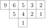
Refer to caption
Figure 1. Hook lengths for λB=(5,4,1)\lambda^{B}=(5,4,1). fλB=56f^{\lambda^{B}}=56.

The final preliminary to proving the main results of this paper is the following lemma. The proof is straightforward and omitted here.

Lemma 2.8.

For w0B∈𝔖nBw_{0}^{B}\in\mathfrak{S}_{n}^{B} and i∈[0,n−1]i\in[0,n-1],

si​w0B​si=w0B.s_{i}w_{0}^{B}s_{i}=w_{0}^{B}.

This indicates a ℤ/n2​ℤ\mathbb{Z}/n^{2}\mathbb{Z}-action on the set R⁡(w0B)R(w_{0}^{B}) defined by

si1si2⋯sin2↦si2⋯sin2si1.s_{i_{1}}s_{i_{2}}\cdots s_{i_{n^{2}}}\mapsto s_{i_{2}}\cdots s_{i_{n^{2}}}s_{i_{1}}.

As with the other machinery discussed in this section, Lemma 2.8 has an analogous (though not identical) statement in type AA which is used in [4].

3. Expectation of Yang-Baxter moves

Consider the set R⁡(w0B)R(w_{0}^{B}) with uniform probability distribution. Let XnBX_{n}^{B} be the random variable on reduced decompositions of w0B∈𝔖nBw_{0}^{B}\in\mathfrak{S}_{n}^{B} which counts the number of Yang-Baxter moves.

Theorem 3.1.

For all n≥3n\geq 3, E⁡(XnB)=2−4/nE(X_{n}^{B})=2-4/n.

Proof.

Fix n≥3n\geq 3. For k>0k>0, let XnB​[j,k]X_{n}^{B}[j,k] be the indicator random variable which determines whether the factor ij​ij+1​ij+2i_{j}i_{j+1}i_{j+2} in a reduced decomposition i1⋯in2i_{1}\cdots i_{n^{2}} in R⁡(w0B)R(w_{0}^{B}) is of either form k⁡(k+1)​kk(k+1)k or (k+1)​k​(k+1)(k+1)k(k+1). Therefore

E⁡(XnB)=∑j=1n2−2∑k=1n−2E⁡(XnB​[j,k]).E(X_{n}^{B})=\sum_{j=1}^{n^{2}-2}\ \sum_{k=1}^{n-2}E(X_{n}^{B}[j,k]).

The variables XnB​[j,k]X_{n}^{B}[j,k] and XnB​[j′,k]X_{n}^{B}[j^{\prime},k] have the same distribution by Lemma 2.8, so in fact

E⁡(XnB)=(n2−2)​∑k=1n−2E⁡(XnB​[1,k]).E(X_{n}^{B})=(n^{2}-2)\sum_{k=1}^{n-2}E(X_{n}^{B}[1,k]).

If XnB​[1,k]​(𝒊)=1X_{n}^{B}[1,k](\mbox{\boldmath$i$})=1 for 𝒊=i1⋯in2∈R(w0B)\mbox{\boldmath$i$}=i_{1}\cdots i_{n^{2}}\in R(w_{0}^{B}), then

𝒊∈{k(k+1)ki4⋯in2,(k+1)k(k+1)i4⋯in2}.\mbox{\boldmath$i$}\in\{k(k+1)ki_{4}\cdots i_{n^{2}},(k+1)k(k+1)i_{4}\cdots i_{n^{2}}\}.

In both cases, i4⋯in2i_{4}\cdots i_{n^{2}} is a reduced decomposition of

wk:=sksk+1skw0B=1¯⋯(k−1)¯(k+2)¯(k+1)¯(k)¯(k+3)¯⋯n¯.w_{k}:=s_{k}s_{k+1}s_{k}w_{0}^{B}=\underline{1}\cdots\underline{(k-1)}\underline{(k+2)}\underline{(k+1)}\underline{(k)}\underline{(k+3)}\cdots\underline{n}.

Notice that wkw_{k} is vexillary for type BB for all kk. Therefore, by Proposition 2.5,

(7) E⁡(XnB)=2​(n2−2)​∑k=1n−2#​R​(wk)#​R​(w0B)=2​(n2−2)​∑k=1n−2fλB​(wk)fλB​(w0B)E(X_{n}^{B})=2(n^{2}-2)\sum_{k=1}^{n-2}\frac{\#R(w_{k})}{\#R(w_{0}^{B})}=2(n^{2}-2)\sum_{k=1}^{n-2}\frac{f^{\lambda^{B}(w_{k})}}{f^{\lambda^{B}(w_{0}^{B})}}

The shifted shapes λB​(w0B)\lambda^{B}(w_{0}^{B}) and λB​(wk)\lambda^{B}(w_{k}) are easy to determine, as the signed permutation uu in Definition 2.3 is n¯⋯1¯\underline{n}\cdots\underline{1} in both cases, so no boxes contain primed entries in the shifted tableau TT. Thus, the shifted shapes are

(8) λB​(w0B)\displaystyle\lambda^{B}(w_{0}^{B}) =\displaystyle= (2​n−1,2​n−3,…,3,1)​ and\displaystyle(2n-1,2n-3,\ldots,3,1)\text{ and}
λB​(wk)\displaystyle\lambda^{B}(w_{k}) =\displaystyle= (2​n−1,2​n−3,…,2​k+5,2​k+1,2​k,2​k−1,…,3,1).\displaystyle(2n-1,2n-3,\ldots,2k+5,2k+1,2k,2k-1,\ldots,3,1).

Recall the hook-length formula of Proposition 2.7, particularly the definition of the hooks hBh^{B} in shifted shapes. The only hook-lengths that do not cancel in the ratio fλB​(wk)/fλB​(w0B)f^{\lambda^{B}(w_{k})}/f^{\lambda^{B}(w_{0}^{B})} are as indicated in Figure 2.

Refer to captionRefer to caption\begin{array}[]{c@{\hspace{.2in}}c}\psfig{file,width}\hfil\hskip 14.45377pt&\hskip 14.45377pt\psfig{file,width}\end{array}

Figure 2. The shifted shapes λB​(w0B)\lambda^{B}(w_{0}^{B}) and λB​(wk)\lambda^{B}(w_{k}) for n=8n=8 and k=2k=2. The shaded boxes are where the hook-lengths are unequal.

Consequently, equation (7) can be written as

(9) E⁡(XnB)=13​(n22)−1​∑k=1n−2Ck,E(X_{n}^{B})=\frac{1}{3}\binom{n^{2}}{2}^{-1}\ \sum_{k=1}^{n-2}C_{k},

where

Ck=3⋅5⋯(2k+3)2⋅4⋯(2k)⋅3⋅5⋯(2n−2k−1)2⋅4⋯(2n−2k−4)⋅(2k+4)(2k+6)⋯(4k+4)(2k+1)(2k+3)⋯(4k+1)⋅(4k+8)(4k+10)⋯(2n+2k+2)(4k+5)(4k+7)⋯(2n+2k−1),C_{k}=\frac{3\cdot 5\cdots(2k+3)}{2\cdot 4\cdots(2k)}\cdot\frac{3\cdot 5\cdots(2n-2k-1)}{2\cdot 4\cdots(2n-2k-4)}\cdot\frac{(2k+4)(2k+6)\cdots(4k+4)}{(2k+1)(2k+3)\cdots(4k+1)}\\ \cdot\frac{(4k+8)(4k+10)\cdots(2n+2k+2)}{(4k+5)(4k+7)\cdots(2n+2k-1)},

and empty products are defined to be 11.

Notice that

Ck+1Ck=(2​k+3)​(4​k+7)​(2​k+1)​(n−k−2)​(n+k+2)(4​k+3)​(k+2)​(2​n+2​k+1)​(2​n−2​k−1)​(k+1)\frac{C_{k+1}}{C_{k}}=\frac{(2k+3)(4k+7)(2k+1)(n-k-2)(n+k+2)}{(4k+3)(k+2)(2n+2k+1)(2n-2k-1)(k+1)}

is a rational function in kk. Therefore, ∑k=1n−2Ck\sum_{k=1}^{n-2}C_{k} is a hypergeometric series. Following the notation in [5], equation (9) can be rewritten as

E⁡(XnB)=13​(n22)−1​C0​(F45​(3/2,7/4,1/2,2−n,2+n3/4,2,1/2+n,1/2−n)−1).E(X_{n}^{B})=\frac{1}{3}\binom{n^{2}}{2}^{-1}C_{0}\left({}_{5}F_{4}\begin{pmatrix}3/2,7/4,1/2,2-n,2+n\\ 3/4,2,1/2+n,1/2-n\end{pmatrix}-1\right).

The hypergeometric series in question can be computed via Dougall’s theorem, as discussed in [7]. The theorem states that

F45​(a,1+a/2,b,c,da/2,1+a−b,1+a−c,1+a−d)=Γ⁡(1+a−b)​Γ​(1+a−c)​Γ​(1+a−d)​Γ​(1+a−b−c−d)Γ⁡(1+a)​Γ​(1+a−b−c)​Γ​(1+a−b−d)​Γ​(1+a−c−d).{}_{5}F_{4}\begin{pmatrix}a,1+a/2,b,c,d\\ a/2,1+a-b,1+a-c,1+a-d\end{pmatrix}\\ =\frac{\Gamma(1+a-b)\Gamma(1+a-c)\Gamma(1+a-d)\Gamma(1+a-b-c-d)}{\Gamma(1+a)\Gamma(1+a-b-c)\Gamma(1+a-b-d)\Gamma(1+a-c-d)}.

It is not immediately obvious that Dougall’s theorem applies to this particular series because of a potential pole. However, the theorem does show that

F45​(3/2,7/4,1/2,2−n,2+x3/4,2,1/2+n,1/2−x){}_{5}F_{4}\begin{pmatrix}3/2,7/4,1/2,2-n,2+x\\ 3/4,2,1/2+n,1/2-x\end{pmatrix} =\displaystyle= Γ⁡(2)​Γ​(1/2+n)​Γ​(1/2−x)​Γ​(n−x−2)Γ⁡(5/2)​Γ​(n)​Γ​(−x)​Γ​(n−x−3/2)\displaystyle\frac{\Gamma(2)\Gamma(1/2+n)\Gamma(1/2-x)\Gamma(n-x-2)}{\Gamma(5/2)\Gamma(n)\Gamma(-x)\Gamma(n-x-3/2)}
=\displaystyle= (−x)n−2​(5/2)n−2(n−1)!​(1/2−x)n−2.\displaystyle\frac{(-x)_{n-2}(5/2)_{n-2}}{(n-1)!(1/2-x)_{n-2}}.

Therefore there is no pole in this situation. Letting xx approach nn shows that the desired hypergeometric series has sum n/2n/2.

Finally,

C0=3⋅3⋅5⋯(2n−1)2⋅4⋯(2n−4)⋅41⋅8⋅10⋯(2n+2)5⋅7⋯(2n−1)=6​n​(n2−1),C_{0}=3\cdot\frac{3\cdot 5\cdots(2n-1)}{2\cdot 4\cdots(2n-4)}\cdot\frac{4}{1}\cdot\frac{8\cdot 10\cdots(2n+2)}{5\cdot 7\cdots(2n-1)}=6n(n^{2}-1),

which completes the proof:

E⁡(XnB)=13​(n22)−1​6​n​(n2−1)​(n/2−1)=2−4/n.E(X_{n}^{B})=\frac{1}{3}\binom{n^{2}}{2}^{-1}6n(n^{2}-1)(n/2-1)=2-4/n.

∎

As suggested earlier, it is appropriate that Yang-Baxter moves are approximately twice as common in elements of R⁡(w0B)R(w_{0}^{B}) as in elements of R⁡(w0)R(w_{0}), as

ℓ⁡(w0B)=n2≈2​(n2)=2​ℓ​(w0).\ell(w_{0}^{B})=n^{2}\approx 2\binom{n}{2}=2\ell(w_{0}).

4. Expectation of 0101 moves

As in the previous section, consider the set R⁡(w0B)R(w_{0}^{B}) with uniform probability distribution. Let YnBY_{n}^{B} be the random variable on reduced decompositions of w0B∈𝔖nBw_{0}^{B}\in\mathfrak{S}_{n}^{B} which counts the number of 0101 moves.

Theorem 4.1.

For all n≥2n\geq 2, E⁡(YnB)=2/(n2−2)E(Y_{n}^{B})=2/(n^{2}-2).

Proof.

As in the proof of Theorem 3.1, let YnB​[j]Y_{n}^{B}[j] be the indicator random variable which determines whether the factor ij​ij+1​ij+2​ij+3i_{j}i_{j+1}i_{j+2}i_{j+3} in a reduced decomposition i1⋯in2i_{1}\cdots i_{n^{2}} in R⁡(w0B)R(w_{0}^{B}) is of either form 01010101 or 10101010. Lemma 2.8 similarly applies, so

E⁡(YnB)=∑j=1n2−3E⁡(YnB​[j])=(n2−3)​E​(YnB​[1]).E(Y_{n}^{B})=\sum_{j=1}^{n^{2}-3}E(Y_{n}^{B}[j])=(n^{2}-3)E(Y_{n}^{B}[1]).

If YnB​[1]​(𝒊)=1Y_{n}^{B}[1](\mbox{\boldmath$i$})=1 for 𝒊=i1⋯in2∈R(w0B)\mbox{\boldmath$i$}=i_{1}\cdots i_{n^{2}}\in R(w_{0}^{B}), then 𝒊i is either 0101i5⋯in20101i_{5}\cdots i_{n^{2}} or 1010i5⋯in21010i_{5}\cdots i_{n^{2}}. The string i5⋯in2i_{5}\cdots i_{n^{2}} is a reduced decomposition of

w′=123¯4¯⋯n¯w^{\prime}=12\underline{3}\underline{4}\cdots\underline{n}

in both situations. As with wkw_{k}, the signed permutation w′w^{\prime} is vexillary for type BB. Therefore

E⁡(YnB)=2​(n2−3)​#​R​(w′)#​R​(w0B)=2​(n2−3)​fλB​(w′)fλB​(w0B).E(Y_{n}^{B})=2(n^{2}-3)\frac{\#R(w^{\prime})}{\#R(w_{0}^{B})}=2(n^{2}-3)\frac{f^{\lambda^{B}(w^{\prime})}}{f^{\lambda^{B}(w_{0}^{B})}}.

The shifted shape λB​(w0B)\lambda^{B}(w_{0}^{B}) is as in equation (8). Applying Definition 2.3 to w′w^{\prime} proceeds as follows:

  1. (1)

    The signed permutation uu is n¯⋯3¯12\underline{n}\cdots\underline{3}12.

  2. (2)

    The vexillary permutation vv is (n−1)n(n−2)(n−3)⋯21(n-1)n(n-2)(n-3)\cdots 21.

  3. (3)

    The partition μ\mu is (n,n−1,…,4,3)(n,n-1,\ldots,4,3).

  4. (4)

    The shifted tableau UU has shape (n,n−1,…,4,3)(n,n-1,\ldots,4,3) and the straight tableau VV has shape (n−1,n−2,…,3,2)(n-1,n-2,\ldots,3,2).

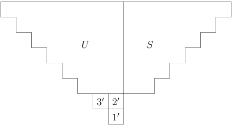
Refer to caption
Figure 3. Step (7) of Definition 2.3 applied to w′w^{\prime}.

Unlike in the cases of w0Bw_{0}^{B} or wkw^{k} in the proof of Theorem 3.1, there will be boxes of TT containing primed numbers, specifically 1′1^{\prime}, 2′2^{\prime}, and 3′3^{\prime}, as in Figure 3. However, removing 1′1^{\prime} leaves a shifted tableau so jeu de taquin is not applied. Similarly, 2′2^{\prime} and then 3′3^{\prime} can each be removed without performing jeu de taquin. Thus

λB​(w′)=(2​n−1,2​n−3,…,7,5).\lambda^{B}(w^{\prime})=(2n-1,2n-3,\ldots,7,5).

Having determined λB​(w′)\lambda^{B}(w^{\prime}), it remains to compute the ratio fλB​(w′)/fλB​(w0B)f^{\lambda^{B}(w^{\prime})}/f^{\lambda^{B}(w_{0}^{B})} via Proposition 2.7. As in the proof of Theorem 3.1, many of the hook-lengths cancel. Figure 4 depicts the only boxes in the two shapes where the hook-lengths differ.

Refer to captionRefer to caption\begin{array}[]{c@{\hspace{.2in}}c}\psfig{file,width}\hfil\hskip 14.45377pt&\hskip 14.45377pt\psfig{file,width}\end{array}

Figure 4. The shifted shapes λB​(w0B)\lambda^{B}(w_{0}^{B}) and λB​(w′)\lambda^{B}(w^{\prime}) for n=8n=8. The shaded boxes indicate unequal hook-lengths.

From here it is not hard to compute that

E⁡(YnB)\displaystyle E(Y_{n}^{B}) =\displaystyle= 2​(n2−3)​(n2−4)!(n2)!⋅3⋅(2​n)⋅(2​n−2)​(2​n)​(2​n+2)2⋅4⋅6\displaystyle 2(n^{2}-3)\frac{(n^{2}-4)!}{(n^{2})!}\cdot 3\cdot(2n)\cdot\frac{(2n-2)(2n)(2n+2)}{2\cdot 4\cdot 6}
=\displaystyle= (n23)−1⋅(2​n)⋅(n−1)​(n)​(n+1)1⋅2⋅3\displaystyle\binom{n^{2}}{3}^{-1}\cdot(2n)\cdot\frac{(n-1)(n)(n+1)}{1\cdot 2\cdot 3}
=\displaystyle= 2n2−2.\displaystyle\frac{2}{n^{2}-2}.

∎

5. Acknowledgments

I am deeply grateful to Vic Reiner for numerous conversations and feedback, and for suggesting the generalization to type BB. Thanks also to Dennis Stanton for his comments regarding Dougall’s theorem.

References

  • [1] S. Billey and T. K. Lam, Vexillary elements in the hyperoctahedral group, J. Alg. Combin. 8 (1998), 139-152.
  • [2] A. Björner and F. Brenti, Combinatorics of Coxeter Groups, Graduate Texts in Mathematics 231231, Springer, New York, 2005.
  • [3] I. G. Macdonald, Notes on Schubert Polynomials, Laboratoire de combinatoire et d’informatique mathématique (LACIM), Université du Québec à Montréal, Montreal, 1991.
  • [4] V. Reiner, Note on the expected number of Yang-Baxter moves applicable to reduced decompositions, Europ. J. Combinatorics 26 (2005), 1019-1021.
  • [5] R. Roy, Binomial identities and hypergeometric series, Amer. Math. Monthly 94 (1987), 36-46.
  • [6] B. E. Sagan, Partially ordered sets with hooklengths - an algorithmic approach, Ph.D. Thesis, M.I.T., 1979.
  • [7] L. J. Slater, Generalized Hypergeometric Functions, Cambridge University Press, Cambridge, 1966.
  • [8] R. P. Stanley, Enumerative Combinatorics, vol. 2, Cambridge Studies in Advanced Mathematics, no. 62, Cambridge University Press, Cambridge, 1999.
  • [9] R. P. Stanley, On the number of reduced decompositions of elements of Coxeter groups, Europ. J. Combinatorics 5 (1984), 359-372.
  • [10] B. E. Tenner, Reduced decompositions and permutation patterns, arXiv:math.CO/0506242.