Szegő polynomials: a view from the Riemann-Hilbert windowThanks: This paper is dedicated to Ed Saff on the occasion of his 60th birthday.

A. Martínez-Finkelshtein Thanks: University of Almería and Instituto Carlos I de Física Teórica y Computacional, Granada University, Spain.

This paper is dedicated to Ed Saff on the occasion of

Abstract

This is an expanded version of the talk given at the conference “Constructive Functions Tech-04”. We survey some recent results on canonical representation and asymptotic behavior of polynomials orthogonal on the unit circle with respect to an analytic weight. These results are obtained using the steepest descent method based on the Riemann-Hilbert characterization of these polynomials.

keywords

Zeros, asymptotics, Riemann-Hilbert problem, Szegő polynomials, Verblunsky coefficients

AMS

33C45

1 Introduction

During the Fall Semester of 2003 I was visiting the Department of Mathematics of the Vanderbilt University, where I had the opportunity to continue my collaboration with Ed Saff. I was very excited with the evolution of the Riemann-Hilbert approach to the asymptotic analysis of orthogonal polynomials, and discussed extensively with Ed the new perspectives. He was the one who posed the question: can this method tell us anything new about such a classical object as the orthogonal polynomials on the unit circle (OPUC, known also as Szegő polynomials), in particular, about their zeros? The question was more on a skeptical side. I was aware of some previous work of the founders of the method, [1], [3], but none of these papers was focused on the description of the zeros of the OPUC’s. So, we started to work and realized that we were able to find curious facts even in the simplest situations. Later on I visited Ken McLaughlin, at that time in Chapel Hill. A two-day discussion at Strong Café (a recommended place) was crucial, and Ken joined the team. This paper is a short and informal report on some of the advances we have had so far.

Let me introduce some notation and describe the setting. For $r>0$ , denote $\mathbb{D}_{r}\stackrel{{\scriptstyle\text{\tiny def}}}{{=}}\{z\in\mathbb{C}:\,|z|<r\}$ , and ${\mathbb{T}}_{r}\stackrel{{\scriptstyle\text{\tiny def}}}{{=}}\{z\in\mathbb{C}:\,|z|=r\}$ . A positive measure $\mu$ on ${\mathbb{T}}_{1}$ has the Lebesgue-Radon-Nikodym decomposition

d\mu(z)=w(z)\,|dz|+d\mu_{s}

(1)

where $\mu_{s}$ is the singular part of $\mu$ with respect to the Lebesgue measure on ${\mathbb{T}}_{1}$ . Throughout, we will consider measures satisfying the Szegő condition

\int_{{\mathbb{T}}_{1}}\log w(z)\,|dz|>-\infty\,,

allowing to define the Szegő function (see e.g. [19, Ch. X, §10.2]):

D(w;z)\stackrel{{\scriptstyle\text{\tiny def}}}{{=}}\exp\left(\frac{1}{4\pi}\,\int_{0}^{2\pi}\log w(e^{i\theta})\,\frac{e^{i\theta}+z}{e^{i\theta}-z}\,d\theta\right)\,.

(2)

This function is piecewise analytic and non-vanishing, defined for $|z|\neq 1$ , and we will denote by $D_{\rm i}$ and $D_{\rm e}$ its values for $|z|<1$ and $|z|>1$ , respectively, given by formula (2). It is easy to verify that

\overline{D_{\rm i}\left(w;\frac{1}{\overline{z}}\right)}=\frac{1}{D_{\rm e}(w;z)}\,,\quad|z|>1\,,

(3)

and for the boundary values we have

w(z)=\frac{D_{\rm i}(w;z)}{D_{\rm e}(w;z)}=\frac{1}{|D_{\rm e}(w;z)|^{2}}\,,\quad z\in{\mathbb{T}}_{1}\,.

(4)

The first equality in (4) can be regarded as a Wiener-Hopf factorization of the weight $w$ , which is a key fact for the forthcoming analysis.

For a nontrivial positive measure $\mu$ on ${\mathbb{T}}_{1}$ there exists a unique sequence of polynomials $\varphi_{n}(z)=\kappa_{n}z^{n}+\text{lower degree terms}$ , $\kappa_{n}>0$ , such that

\oint_{{\mathbb{T}}_{1}}\varphi_{n}(z)\overline{\varphi_{m}(z)}\,d\mu(z)=\delta_{mn}\,,\quad m,n=0,1,\dots

(5)

We denote by $\Phi_{n}(z)\stackrel{{\scriptstyle\text{\tiny def}}}{{=}}\varphi_{n}(z)/\kappa_{n}$ the corresponding monic orthogonal polynomials. They satisfy the Szegő recurrence

\Phi_{n+1}(z)=z\Phi_{n}(z)-\overline{\alpha_{n}}\,\Phi_{n}^{*}(z)\,,\quad\Phi_{0}(z)\equiv 1\,,

where we use the standard notation $\Phi_{n}^{*}(z)\stackrel{{\scriptstyle\text{\tiny def}}}{{=}}z^{n}\overline{\Phi_{n}(1/\overline{z})}$ . The parameters $\alpha_{n}=-\overline{\Phi_{n+1}(0)}$ are called Verblunsky coefficients (also reflection coefficients or Schur parameters) and satisfy $\alpha_{n}\in\mathbb{D}_{1}$ for $n=0,1,2,\dots$ . Furthermore, $\mu\leftrightarrow\{\alpha_{n}\}$ is a bijection; the map $\mu\rightarrow\{\alpha_{n}\}$ is an inverse problem, and it is known to be difficult. In [18] there is a thorough discussion of several techniques to tackle this problem. Recently, the Riemann-Hilbert approach, not described in [18], proved to be very promising in this context also (see [1], [3], [6], [13]). The main goal of this paper is a further discussion of how this method can shed new light on the study of the asymptotics of the Szegő polynomials. We are not going to provide detailed proofs that can be found elsewhere (the references are included), the aim is to show the method in action and to discuss some new results in two apparently simple situations.

The structure of the paper is as follows. Section 2 is devoted to the case when $D(w;\cdot)$ is non vanishing and has an analytic extension across ${\mathbb{T}}_{1}$ . The main role here is played by the scattering function¹¹ 1 Function $1/{\mathcal{S}}$ is denoted in [17] by $r$ , and in [18, Section 6.2] by $b$ . It corresponds also to the scattering matrix in [9]. I prefer to follow the notation of [12].

{\mathcal{S}}(w;z)\stackrel{{\scriptstyle\text{\tiny def}}}{{=}}D_{\rm i}(w;z)D_{\rm e}(w;z)\,,

(6)

meromorphic in an annulus, containing ${\mathbb{T}}_{1}$ , and which, via its iterated Cauchy transforms, allows to write some canonical series representing $\varphi_{n}$ ’s. In this situation convergence is always exponentially fast, and the Riemann-Hilbert analysis is particularly simple and transparent. Only some of the multiple corollaries of the canonical representation are discussed; a more thorough analysis is contained in [12]. In Section 3 we look at the situation when the original analytic and nonvanishing weight has been modified by a factor having a finite number of zeros on the unit circle. Now the behavior of the zeros of $\Phi_{n}$ ’s is qualitatively different: most of them cluster at ${\mathbb{T}}_{1}$ , and only a finite number stays within the disc $\mathbb{D}_{1}$ . The method of Section 2 must be modified now in order to handle the zeros of the weight: a local analysis plays the major role. The exposition here is much more sketchy; in this sense, more than a detailed view this window gives us a glimpse of the possible techniques and results. At any rate, the main goal is to persuade the reader that the Riemann-Hilbert analysis is a powerfull technique, that deserves to be in the toolbox of those interested in orthogonal polynomials on the unit circle.

2 Analytic and nonvanishing weight

Any analysis of OPUC’s can be started either from the orthogonality measure $\mu$ or from the sequence of the Verblunsky coefficients $\{\alpha_{n}\}$ . Let us assume that the sequence of the Verblunsky coefficients has an exponential decay:

\rho\stackrel{{\scriptstyle\text{\tiny def}}}{{=}}\varlimsup_{n\to\infty}|\alpha_{n}|^{1/n}\,.

(7)

Nevai-Totik [15] proved that this situation is characterized by the following conditions on $\mu$ : in the decomposition (1), $\mu_{s}=0$ , measure $\mu$ satisfies the Szegő condition, and

\rho=\inf\{0<r<1:\,D_{\rm e}(w;z)\text{ is holomorphic in }|z|>r\}\,.

(8)

Taking into account (3) we see that the first identity in (4) can be regarded as an analytic extension of the weight $w$ . With this definition of $w$ (which we use in the sequel) we can say equivalently that

\rho=\inf\{0<r<1:\,1/w(z)\text{ is holomorphic in }r<|z|<1/r\}\,,

(9)

and both circles ${\mathbb{T}}_{\rho}$ and ${\mathbb{T}}_{1/\rho}$ contain singularities of $1/w$ . In this situation the well-known Szegő asymptotic formula

\lim_{n\to\infty}\varphi_{n}^{*}(z)=\frac{1}{D_{\rm i}(w;z)}\,,\quad z\in\mathbb{D}_{1}\,,

can be continued analytically through the unit circle ${\mathbb{T}}_{1}$ and is valid locally uniformly in $\mathbb{D}_{1/\rho}$ . It shows that the number of zeros of $\{\varphi_{n}\}$ on compact subsets of $\mathbb{D}_{1}\setminus\overline{\mathbb{D}}_{\rho}$ remains uniformly bounded, and these zeros are attracted by the zeros of $D_{\rm e}$ in $\rho<|z|<1$ (Nevai-Totik points in the terminology of B. Simon [16]). Numerical experiments show that the vast majority of zeros gather at the “critical circle” ${\mathbb{T}}_{\rho}$ . This fact was justified theoretically by Mhaskar and Saff [14], who using potential theory arguments showed that for any subsequence $\{n_{k}\}\subset\mathbb{N}$ satisfying

\rho=\lim|\alpha_{n_{k}}|^{1/n_{k}}\,,

the zeros of $\{\varphi_{n_{k}+1}\}$ distribute asymptotically uniformly in the weak-star sense on ${\mathbb{T}}_{\rho}$ .

The behavior of the zeros inside $\mathbb{D}_{\rho}$ can be intriguing. Although approaching in mass the critical circle ${\mathbb{T}}_{\rho}$ as predicted by Mhaskar and Saff, some of them still may remain inside and follow interesting patterns. Even the convergence to the circle ${\mathbb{T}}_{\rho}$ is different for different measures. Can we give a full description of this behavior in terms of the weight of orthogonality? The answer is positive, and the description will involve a sequence of iterates of certain Hankel and Toeplitz operators with symbols depending on the scattering function ${\mathcal{S}}$ introduced in (6). It is a consequence of a canonical representation of the Szegő polynomials, found by means of the Riemann-Hilbert characterization.

2.1 Steepest descent analysis and canonical representation for orthogonal polynomials

The starting point of all the analysis is the fact that under assumption (7) conditions (5) can be rewritten in terms of a non-hermitian orthogonality for $\varphi_{n}$ and $\varphi_{n}^{*}$ :

	$\displaystyle\oint_{{\mathbb{T}}_{1}}\varphi_{n}(z)z^{n-k-1}\,\frac{w(z)}{z^{n}}dz$	$\displaystyle=0,\quad\text{for }k=0,1,\dots,n-1\,,$
	$\displaystyle\oint_{{\mathbb{T}}_{1}}\varphi^{*}_{n-1}(z)z^{k}\,\frac{w(z)}{z^{n}}\,dz$	$\displaystyle=\begin{cases}0,&k=0,1,\dots,n-2,\\ i/\kappa_{n-1},&k=n-1\,.\end{cases}$

Here and in what follows, all the circles ${\mathbb{T}}_{\alpha}$ , $\alpha>0$ , are oriented counterclockwise; with this orientation we talk about the “ $+$ ” and the “ $-$ ” side of ${\mathbb{T}}_{\alpha}$ referring to its inner and outer boundary points, respectively. Analogously, $f_{+}$ and $f_{-}$ are the corresponding boundary values on ${\mathbb{T}}_{\alpha}$ for any function $f$ for which these limits exist. By standard arguments (see e.g. [1] or [7], as well as the seminal paper [8] where the Riemann-Hilbert approach to orthogonal polynomials started),

Y(z)=\begin{pmatrix}\Phi_{n}(z)&\displaystyle\dfrac{1}{2\pi i}\,\oint_{{\mathbb{T}}_{1}}\dfrac{\Phi_{n}(t)w(t)\,dt}{t^{n}(t-z)}\\ -2\pi\kappa_{n-1}\varphi^{*}_{n-1}(z)&-\,\displaystyle\dfrac{\kappa_{n-1}}{i}\,\oint_{{\mathbb{T}}_{1}}\dfrac{\varphi^{*}_{n-1}(t)w(t)\,dt}{t^{n}(t-z)}\end{pmatrix}

is a unique solution of the following Riemann-Hilbert problem: $Y$ is holomorphic in $\mathbb{C}\setminus{{\mathbb{T}}_{1}}$ ,

Y_{+}(t)=Y_{-}(t)\,\begin{pmatrix}1&w(t)/t^{n}\\ 0&1\end{pmatrix}\,,\quad z\in{\mathbb{T}}_{1}\,,\quad\text{and}\quad\lim_{z\to\infty}Y(z)\,\begin{pmatrix}z^{-n}&0\\ 0&z^{n}\end{pmatrix}=I\,,

(10)

where $I$ is the $2\times 2$ identity matrix.

This is the starting position for the steepest descent analysis as described in [7] (see also [10]), which consists in performing a series of explicit and reversible steps in order to arrive at an equivalent problem, which is solvable, at least in an asymptotic sense. Since these steps are almost standard, they will be described very schematically. We will use the following notation: $\sigma_{3}=\begin{pmatrix}1&0\\ 0&-1\end{pmatrix}$ is the Pauli matrix, and for any non-zero $x$ and integer $m$ , $x^{\sigma_{3}}=\begin{pmatrix}x&0\\ 0&1/x\end{pmatrix}$ and $x^{m\sigma_{3}}=(x^{m})^{\sigma_{3}}$ .

Step 1: Define

H(z)\stackrel{{\scriptstyle\text{\tiny def}}}{{=}}\begin{cases}z^{-n\sigma_{3}},&\text{if }|z|>1,\\ I,&\text{if }|z|<1,\end{cases}

(11)

and put $T(z)\stackrel{{\scriptstyle\text{\tiny def}}}{{=}}Y(z)\,H(z)$ . Then $T$ is holomorphic in $\mathbb{C}\setminus{{\mathbb{T}}_{1}}$ ; this transformation normalizes the behavior at infinity: $\lim_{z\to\infty}T(z)=I$ . The price we pay is the oscillatory behavior of the new jump matrix on ${\mathbb{T}}_{1}$ :

T_{+}(t)=T_{-}(t)\,\begin{pmatrix}t^{n}&w(t)\\ 0&t^{-n}\end{pmatrix}\,,\quad t\in{\mathbb{T}}_{1}\,.

We get rid of these oscillations in the next transformation, taking advantage of the analyticity of its entries in the annulus.

Step 2: Choose an arbitrary $r$ , $\rho<r<1$ , that we fix for what follows; it determines the regions (Figure 1)

	$\displaystyle\Omega_{0}$	$\displaystyle=\{z:\,\|z\|<r\},\qquad\Omega_{\infty}=\{z:\,\|z\|>1/r\},$
	$\displaystyle\Omega_{+}$	$\displaystyle=\{z:\,r<\|z\|<1\},\qquad\Omega_{-}=\{z:\,1<\|z\|<1/r\}.$

\begin{overpic}[nice_case1bis] \put(79.0,24.0){${\mathbb{T}}_{1}$} \put(70.0,32.0){${\mathbb{T}}_{r}$} \put(90.0,17.0){${\mathbb{T}}_{1/r}$} \put(60.0,60.0){$\Omega_{0}$} \put(69.0,69.0){$\Omega_{+}$} \put(78.0,78.0){$\Omega_{-}$} \put(90.0,90.0){$\Omega_{\infty}$} \put(54.0,38.0){\small$r$} \put(27.0,10.0){\small$1/r$} \put(20.0,41.0){\small$1$} \end{overpic}

Fig. 1: Opening lenses.

Define $U(z)\stackrel{{\scriptstyle\text{\tiny def}}}{{=}}T(z)K(z)$ , where

K(z)\stackrel{{\scriptstyle\text{\tiny def}}}{{=}}\begin{cases}I,&\text{if }z\in\Omega_{0}\cup\Omega_{\infty},\\ \begin{pmatrix}1&0\\ z^{n}/w(z)&1\end{pmatrix}^{-1}\,,&\text{if }z\in\Omega_{+},\\ \begin{pmatrix}1&0\\ 1/(z^{n}w(z))&1\end{pmatrix}\,,&\text{if }z\in\Omega_{-}.\end{cases}

(12)

Then $U$ is holomorphic in $\mathbb{C}\setminus\left({{\mathbb{T}}_{r}}\cup{{\mathbb{T}}_{1}}\cup{{\mathbb{T}}_{1/r}}\right)$ . We have not modified its behavior at infinity, but now

U_{+}(t)=U_{-}(t)\,J_{U}(t),\quad t\in\left({{\mathbb{T}}_{r}}\cup{{\mathbb{T}}_{1}}\cup{{\mathbb{T}}_{1/r}}\right),

where

J_{U}(t)=\begin{cases}\begin{pmatrix}0&w(t)\\ -1/w(t)&0\end{pmatrix},&\text{if }t\in{{\mathbb{T}}_{1}},\\ \begin{pmatrix}1&0\\ t^{n}/w(t)&1\end{pmatrix},&\text{if }t\in{{\mathbb{T}}_{r}},\\ \begin{pmatrix}1&0\\ 1/(t^{n}w(t))&1\end{pmatrix},&\text{if }t\in{{\mathbb{T}}_{1/r}}.\end{cases}

The jump on ${\mathbb{T}}_{r}$ and ${\mathbb{T}}_{1/r}$ is exponentially close to the identity, which is convenient to our purposes. We have to deal now with the relevant jump on the unit circle.

Step 3: The Szegő functions $D_{\rm i}$ and $D_{\rm e}$ have been introduced in (2). Define

\tau\stackrel{{\scriptstyle\text{\tiny def}}}{{=}}\frac{1}{D_{\rm i}(w;0)}=D_{\rm e}(w;\infty)=\exp\left(-\frac{1}{4\pi}\,\int_{0}^{2\pi}\log w(e^{i\theta})\,d\theta\right)>0\,.

(13)

Hence, if we introduce the geometric mean

\mathcal{G}[w]\stackrel{{\scriptstyle\text{\tiny def}}}{{=}}\exp\left(\frac{1}{2\pi}\int_{0}^{2\pi}\log\left(w\left(e^{i\theta}\right)\,d\theta\right)\right)\,,

(14)

then $\tau=\left(\mathcal{G}[w]\right)^{-1/2}$ .

It is straightforward to check that the piece-wise analytic matrix-valued function

N(z)=N(w;z)\stackrel{{\scriptstyle\text{\tiny def}}}{{=}}\begin{cases}\begin{pmatrix}D_{\rm e}(w;z)/\tau&0\\ 0&\tau/D_{\rm e}(w;z)\end{pmatrix},&\text{if }|z|>1\,,\\ \begin{pmatrix}0&D_{\rm i}(w;z)/\tau\\ -\tau/D_{\rm i}(w;z)&0\end{pmatrix},&\text{if }|z|<1\,,\end{cases}

(15)

is invertible, and has the same jumps on ${\mathbb{T}}_{1}$ as $U(z)$ . This motivates to make a new transformation, defining $S(z)\stackrel{{\scriptstyle\text{\tiny def}}}{{=}}U(z)N^{-1}(z)$ . Matrix $S$ is holomorphic in $\mathbb{C}\setminus({{\mathbb{T}}_{r}}\cup{{\mathbb{T}}_{1}}\cup{{\mathbb{T}}_{1/r}})$ ,

\lim_{z\to\infty}S(z)=I,

and

S_{+}(t)=S_{-}(t)\,J_{S}(t),\quad t\in{{\mathbb{T}}_{r}}\cup{{\mathbb{T}}_{1}}\cup{{\mathbb{T}}_{1/r}},

(16)

where

J_{S}(t)=N_{-}J_{U}N_{+}^{-1}=\begin{cases}I,&\text{if }t\in{{\mathbb{T}}_{1}},\\ \begin{pmatrix}1&-t^{n}{\mathcal{S}}(w;t)/\tau^{2}\\ 0&1\end{pmatrix},&\text{if }t\in{{\mathbb{T}}_{r}},\\ \begin{pmatrix}1&0\\ \tau^{2}/(t^{n}{\mathcal{S}}(w;t))&1\end{pmatrix},&\text{if }t\in{{\mathbb{T}}_{1/r}}.\end{cases}

(17)

Our main character, ${\mathcal{S}}$ , has entered the picture!

Summarizing, we have

Y(z)=S(z)N(z)K^{-1}(z)H^{-1}(z)\,.

(18)

Here $H$ , $K$ and $N$ are explicitly defined in (11), (12) and (15), respectively. About $S$ we know only that it is piece-wise analytic and satisfies the jump condition (16)–(17). A feature of this situation is that we can write a formula for $S$ in terms of a series of iterates of some Cauchy operators acting on the space of holomorphic functions in $\mathbb{C}\setminus({{\mathbb{T}}_{r}}\cup{{\mathbb{T}}_{1/r}})$ with continuous boundary values. Indeed, let us denote

S=\begin{pmatrix}S_{11}&S_{12}\\ S_{21}&S_{22}\end{pmatrix}\,,

and look at the equations given by the jumps on ${\mathbb{T}}_{r}$ . According to (17), the first column is analytic across this circle, while the second column has an additive jump equal to the first column times $-t^{n}{\mathcal{S}}(w;t)/\tau^{2}$ . So, if we define the operator

\mathcal{M}_{n}^{\rm i}(f)(z)\stackrel{{\scriptstyle\text{\tiny def}}}{{=}}-\frac{1}{2\pi i\,\tau^{2}}\,\oint_{{{\mathbb{T}}_{r}}}f_{-}(t)\,\frac{{\mathcal{S}}(w;t)\,t^{n}}{t-z}\,dt\,,

where $f_{-}$ denotes the exterior boundary values of the function $f$ on ${\mathbb{T}}_{r}$ , then taking into account the behavior at infinity and Sokhotsky-Plemelj’s theorem we get that

\displaystyle S_{12}=\mathcal{M}_{n}^{\rm i}(S_{11})\,,\quad S_{22}=1+\mathcal{M}_{n}^{\rm i}(S_{21})\,.

(19)

Analogously, with

\mathcal{M}_{n}^{\rm e}(f)(z)\stackrel{{\scriptstyle\text{\tiny def}}}{{=}}\frac{\tau^{2}}{2\pi i}\,\oint_{{{\mathbb{T}}_{1/r}}}f_{-}(t)\,\frac{1}{{\mathcal{S}}(w;t)\,t^{n}\,(t-z)}\,dt\,,

where $f_{-}$ denotes the exterior boundary values of the function $f$ on ${\mathbb{T}}_{1/r}$ , we have again

\displaystyle S_{11}=1+\mathcal{M}_{n}^{\rm e}(S_{12})\,,\quad S_{21}=\mathcal{M}_{n}^{\rm e}(S_{22})\,.

(20)

By (19), (20), functions $S_{ij}$ satisfy the following integral equations:

	$\displaystyle(I-\mathcal{M}_{n}^{\rm e}\circ\mathcal{M}_{n}^{\rm i})S_{11}$	$\displaystyle=1\,,\qquad(I-\mathcal{M}_{n}^{\rm i}\circ\mathcal{M}_{n}^{\rm e})S_{12}=\mathcal{M}_{n}^{\rm i}(1)\,,$
	$\displaystyle(I-\mathcal{M}_{n}^{\rm e}\circ\mathcal{M}_{n}^{\rm i})S_{21}$	$\displaystyle=\mathcal{M}_{n}^{\rm e}(1)\,,\qquad(I-\mathcal{M}_{n}^{\rm i}\circ\mathcal{M}_{n}^{\rm e})S_{22}=1\,,$

where $I$ is the identity operator. Straightforward bounds show that there exists a constant $C>0$ depending on $r$ only, such that

\begin{split}\left|\mathcal{M}_{n}^{\rm i}(f)(z)\right|&\leq C\,r^{n}\,\frac{\|f_{-}\|_{{\mathbb{T}}_{r}}}{\left||z|-r\right|}\,,\qquad z\notin{\mathbb{T}}_{r}\,,\\ \left|\mathcal{M}_{n}^{\rm e}(f)(z)\right|&\leq C\,r^{n}\,\frac{\|f_{-}\|_{{\mathbb{T}}_{1/r}}}{\left||z|-1/r\right|}\,,\qquad z\notin{\mathbb{T}}_{1/r}\,,\end{split}

(21)

where $\|\cdot\|_{\gamma}$ is the $\sup$ -norm on $\gamma$ ; in the sequel we use $C$ to denote some irrelevant constants, different in each appearance, whose dependence or independence on the parameters will be stated explicitly. Thus, we can invert these operators using convergent Neumann series,

	$\displaystyle S_{11}$	$\displaystyle=\left(\sum_{k=0}^{\infty}\left(\mathcal{M}_{n}^{\rm e}\circ\mathcal{M}_{n}^{\rm i}\right)^{k}\right)(1)\,,\qquad S_{12}=\left(\sum_{k=0}^{\infty}\left(\mathcal{M}_{n}^{\rm i}\circ\mathcal{M}_{n}^{\rm e}\right)^{k}\circ\mathcal{M}_{n}^{\rm i}\right)(1)\,,$
	$\displaystyle S_{21}$	$\displaystyle=\left(\sum_{k=0}^{\infty}\left(\mathcal{M}_{n}^{\rm e}\circ\mathcal{M}_{n}^{\rm i}\right)^{k}\circ\mathcal{M}_{n}^{\rm e}\right)(1)\,,\qquad S_{22}=\left(\sum_{k=0}^{\infty}\left(\mathcal{M}_{n}^{\rm i}\circ\mathcal{M}_{n}^{\rm e}\right)^{k}\right)(1)\,.$

In order to make this somewhat more explicit, let us define recursively two sequence of functions:

\begin{split}f_{n}^{(0)}&\stackrel{{\scriptstyle\text{\tiny def}}}{{=}}1\,,\quad f_{n}^{(1)}\stackrel{{\scriptstyle\text{\tiny def}}}{{=}}\mathcal{M}_{n}^{\rm i}(1)\,,\quad\text{and}\quad f_{n}^{(2k)}\stackrel{{\scriptstyle\text{\tiny def}}}{{=}}\mathcal{M}_{n}^{\rm e}(f_{n}^{(2k-1)})\,,\quad f_{n}^{(2k+1)}\stackrel{{\scriptstyle\text{\tiny def}}}{{=}}\mathcal{M}_{n}^{\rm i}(f_{n}^{(2k)})\,,\quad k\in\mathbb{N}\,,\\ g_{n}^{(0)}&\stackrel{{\scriptstyle\text{\tiny def}}}{{=}}1\,,\quad g_{n}^{(1)}\stackrel{{\scriptstyle\text{\tiny def}}}{{=}}\mathcal{M}_{n}^{\rm e}(1)\,,\quad\text{and}\quad g_{n}^{(2k)}\stackrel{{\scriptstyle\text{\tiny def}}}{{=}}\mathcal{M}_{n}^{\rm i}(g_{n}^{(2k-1)})\,,\quad g_{n}^{(2k+1)}\stackrel{{\scriptstyle\text{\tiny def}}}{{=}}\mathcal{M}_{n}^{\rm e}(g_{n}^{(2k)})\,,\quad k\in\mathbb{N}\,.\end{split}

Then

\begin{split}S_{11}(n;z)&=\sum_{k=0}^{\infty}f_{n}^{(2k)}(z)\,,\quad S_{21}(n;z)=\sum_{k=0}^{\infty}g_{n}^{(2k+1)}(z)\,,\quad\text{ for }|z|\neq 1/r\,,\\ S_{12}(n;z)&=\sum_{k=0}^{\infty}f_{n}^{(2k+1)}(z)\,,\quad S_{22}(n;z)=\sum_{k=0}^{\infty}g_{n}^{(2k)}(z)\,,\quad\text{ for }|z|\neq r\,.\end{split}

All these series are uniformly and absolutely convergent in their domains. Moreover, straightforward bounds on the Cauchy transform show that there exists a constant $C>0$ depending on $r$ only, such that for $i=1,2$ ,

|S_{i1}(z)|\leq\frac{C}{||z|-1/r|}\,,\text{ for }|z|\neq 1/r\,,\quad\text{and}\quad|S_{i2}(z)|\leq\frac{C}{||z|-r|}\,,\text{ for }|z|\neq r\,.

We emphasize that in each of the regions above functions $S_{ij}$ have their own meaning, and are not obtained in general by analytic continuation from one domain to another.

Once we have computed $S$ , we may replace its expression in (18) in order to find $Y$ . It should be performed independently in each region. For instance, in the domain $\Omega_{\infty}$ , $N(z)=\left(D_{\rm e}(w;z)/\tau\right)^{\sigma_{3}}$ , $K(z)=I$ , $H(z)=z^{-n\sigma_{3}}$ , so that

Y(z)=S(z)(z^{n}D_{\rm e}(w;z)/\tau)^{\sigma_{3}}=\begin{pmatrix}S_{11}(n;z)z^{n}D_{\rm e}(w;z)/\tau&S_{12}(n;z)\tau/(z^{n}D_{\rm e}(w;z))\\ S_{21}(n;z)z^{n}D_{\rm e}(w;z)/\tau&S_{22}(n;z)\tau/(z^{n}D_{\rm e}(w;z))\end{pmatrix}\,.

Analogous computations are easily completed in the rest of the regions.

All the information about the parameters of the orthogonal polynomials is codified in the first column of $Y$ : its $(1,1)$ entry gives us $\Phi_{n}$ , that evaluated at $z=0$ yields the Verblunsky coefficients, while the $(2,1)$ entry at $z=0$ is related to the leading coefficient $\kappa$ : $Y_{21}(0)=-2\pi\kappa_{n-1}^{2}$ . Hence, we have obtained the following theorem, that has been proved in [12]:

Theorem 1.

Let $w$ be a strictly positive analytic weight on the unit circle ${\mathbb{T}}_{1}$ , the constant $\rho$ as defined in (8)–(9), and constant $r$ with $\rho<r<1$ fixed. Then with the notations introduced above, for every $n\in\mathbb{N}$ sufficiently large the following formulas hold:

$\displaystyle i)$	$\displaystyle\qquad\Phi_{n}(z)=\begin{cases}\tau^{-1}z^{n}D_{\rm e}(w;z)\,S_{11}(n;z)\,,&\text{if }\|z\|>1/r\,;\\ \tau^{-1}z^{n}D_{\rm e}(w;z)\,S_{11}(n;z)-\dfrac{\tau\,S_{12}(n;z)}{D_{\rm i}(w;z)}\,,&\text{if }r<\|z\|<1/r\,;\\ -\dfrac{\tau\,S_{12}(n;z)}{D_{\rm i}(w;z)}\,,&\text{if }\|z\|<r\,.\end{cases}$	(22)
$\displaystyle ii)$	$\displaystyle\qquad\overline{\alpha_{n}}=\tau^{2}S_{12}(n+1;0)\,.$	(23)
$\displaystyle iii)$	$\displaystyle\qquad\kappa_{n}^{2}=\frac{\tau^{2}}{2\pi}\,S_{22}(n+1;0)\,.$	(24)

Remark: It is easily seen that the method we have just described is valid also if we replace the condition of positivity of $w$ on ${\mathbb{T}}_{1}$ by the requirement that its winding number on ${\mathbb{T}}_{1}$ is zero. In such a case we can assure that $\deg\Phi_{n}=n$ only for sufficiently large $n$ ’s, but the rest of the argument remains the same.

Before we analyze some implications of these formulas let us look more carefully at the scattering function ${\mathcal{S}}$ and at the iterates of its Cauchy transforms used in the definition of $S$ . Following notation of [18, Section 6.2], let

\log w(z)=\sum_{k\in\mathbb{Z}}\hat{L}_{k}z^{k}

be the Laurent expansion (equivalently, the Fourier series) for $\log w$ . Then straightforward computation shows that

{\mathcal{S}}(w;z)=\exp\left(\sum_{k=1}^{+\infty}\left(\hat{L}_{k}z^{k}-\hat{L}_{-k}z^{-k}\right)\right)=\exp\left(\sum_{k=1}^{+\infty}\left(\hat{L}_{k}z^{k}-\overline{\hat{L}_{k}}z^{-k}\right)\right)\,.

Let

{\mathcal{S}}(w;z)=\sum_{k=-\infty}^{+\infty}\left({\mathcal{S}}\right)_{k}z^{k}\quad\text{and}\quad\frac{1}{{\mathcal{S}}(w;z)}=\sum_{k=-\infty}^{+\infty}\left(\frac{1}{{\mathcal{S}}}\right)_{k}z^{k}

(25)

be the Laurent expansions of ${\mathcal{S}}$ and $1/{\mathcal{S}}$ in the annulus $\rho<|z|<1/\rho$ , respectively. Taking into account that $|{\mathcal{S}}(w;z)|=1$ on ${\mathbb{T}}_{1}$ ,

\left(\frac{1}{{\mathcal{S}}}\right)_{k}=\overline{\left({\mathcal{S}}\right)_{-k}}\,,\quad\ \text{and}\quad\sum_{k=-\infty}^{+\infty}\left({\mathcal{S}}\right)_{k+m}\overline{\left({\mathcal{S}}\right)_{k}}=\begin{cases}1,&\text{if }m=0,\\ 0,&\text{if }m\in\mathbb{Z}\setminus\{0\}\,.\end{cases}

(26)

Denote by $H^{2}_{+}$ the Hardy class, and $H_{-}^{2}\stackrel{{\scriptstyle\text{\tiny def}}}{{=}}L^{2}\ominus H^{2}_{+}$ . Let us denote by $\mathcal{P}_{+}$ and $\mathcal{P}_{-}$ the Riesz projections onto $H^{2}_{+}$ and $H^{2}_{-}$ , respectively, and $\sigma_{n}(z)\stackrel{{\scriptstyle\text{\tiny def}}}{{=}}z^{n}{\mathcal{S}}(w;z)$ . Then

\mathcal{P}_{+}(\sigma_{n})(z)=\sum_{k=-n}^{+\infty}\left({\mathcal{S}}\right)_{k}z^{k+n}\,,\qquad\mathcal{P}_{-}(\sigma_{n})(z)=\sum_{k<-n}\left({\mathcal{S}}\right)_{k}z^{k+n}\,.

In particular,

f_{n}^{(1)}(z)=\mathcal{M}_{n}^{\rm i}(1)=\begin{cases}\displaystyle-\frac{1}{\tau^{2}}\,\mathcal{P}_{+}(\sigma_{n})(z)=-\frac{1}{\tau^{2}}\,\sum_{k=-n}^{+\infty}\left({\mathcal{S}}\right)_{k}z^{k+n}\in H_{+}^{2}\,,&\text{if }|z|<r\,,\\ \displaystyle\frac{1}{\tau^{2}}\,\mathcal{P}_{-}(\sigma_{n})(z)=\frac{1}{\tau^{2}}\,\sum_{k<-n}\left({\mathcal{S}}\right)_{k}z^{k+n}\in H^{2}_{-}\,,&\text{if }|z|>r\,.\end{cases}

The series in the right hand side converge locally uniformly. Observe also that

f_{n}^{(1)}(0)=-\frac{1}{\tau^{2}}\,\left({\mathcal{S}}\right)_{-n}=-\frac{1}{\tau^{2}}\,\overline{\left(\frac{1}{{\mathcal{S}}}\right)_{n}}\,.

(27)

If we introduce the following composition of Hankel and Toeplitz operators, having $\sigma_{n}^{\pm 1}$ as a symbol,

\mathcal{H}_{n}^{\pm}:\,H^{2}_{-}\mapsto H^{2}_{\pm}\,,\quad\text{given by }\quad\mathcal{H}_{n}^{+}(f)=-\mathcal{P}_{+}(\sigma_{n}\mathcal{P}_{-}(\sigma_{n}^{-1}f))\,,\quad\mathcal{H}_{n}^{-}(f)=\mathcal{P}_{-}(\sigma_{n}\mathcal{P}_{-}(\sigma_{n}^{-1}f))\,,

then

f_{n}^{(2k+1)}=\begin{cases}\mathcal{H}_{n}^{+}(f_{n,-}^{(2k-1)})\,,&\text{if }|z|<r\,,\\ \mathcal{H}_{n}^{-}(f_{n,-}^{(2k-1)})\,,&\text{if }|z|>r\,,\end{cases}

where $f_{n,-}^{(2k-1)}$ represents the values of $f_{n}^{(2k-1)}$ in $\mathbb{C}\setminus\overline{\mathbb{D}_{r}}$ .

For $g_{n}^{(k)}$ we can obtain analogous formulas:

g_{n}^{(2)}(z)=\mathcal{M}_{n}^{\rm i}(g_{n}^{(1)})=\begin{cases}\displaystyle-\tau^{-2}\,\mathcal{P}_{+}(\sigma_{n}g_{n}^{(1)})(z)=-\mathcal{P}_{+}(\sigma_{n}\mathcal{P}_{+}(\sigma_{n}^{-1}))(z)\,,&\text{if }|z|<r\,,\\ \displaystyle\tau^{-2}\,\mathcal{P}_{-}(\sigma_{n}g_{n}^{(1)})(z)=\mathcal{P}_{-}(\sigma_{n}\mathcal{P}_{+}(\sigma_{n}^{-1}))(z)\,,&\text{if }|z|>r\,,\end{cases}

and

g_{n}^{(2k+2)}=\begin{cases}\mathcal{H}_{n}^{+}(g_{n,-}^{(2k)})\,,&\text{if }|z|<r\,,\\ \mathcal{H}_{n}^{-}(g_{n,-}^{(2k)})\,,&\text{if }|z|>r\,.\end{cases}

For instance, taking into account (26), for $|z|<r$ ,

\begin{split}g_{n}^{(2)}(z)&=-\mathcal{P}_{+}(\sigma_{n}\mathcal{P}_{+}(\sigma_{n}^{-1}))(z)=-\mathcal{P}_{+}\left(\left(\sum_{j=-\infty}^{+\infty}\left({\mathcal{S}}\right)_{j}z^{j+n}\right)\left(\sum_{k=n}^{+\infty}\left(\frac{1}{{\mathcal{S}}}\right)_{k}\,z^{k-n}\right)\right)\\ &=-\sum_{k\leq j,\;k\leq-n}\left({\mathcal{S}}\right)_{j}\overline{\left({\mathcal{S}}\right)_{k}}\,z^{j-k}=-\sum_{m=0}^{+\infty}\left(\sum_{k\leq-n}\left({\mathcal{S}}\right)_{k+m}\overline{\left({\mathcal{S}}\right)_{k}}\right)\,z^{m}\,,\end{split}

and by identities in (26) we can rewrite last formula as

1+g_{n}^{(2)}(z)=\sum_{m=0}^{+\infty}\left(\sum_{k>-n}\left({\mathcal{S}}\right)_{k+m}\overline{\left({\mathcal{S}}\right)_{k}}\right)z^{m}\,,\quad|z|<r\,.

(28)

Remarks: There are some further relations and equivalent expressions that an interested reader can easily derive. For instance, if we introduce the operator $\mathcal{T}_{n}$ on $L^{2}$ with kernel

T_{n}(i,j)\stackrel{{\scriptstyle\text{\tiny def}}}{{=}}\sum_{s=0}^{+\infty}\left({\mathcal{S}}\right)_{-(s+n+1+j)}\left(\frac{1}{{\mathcal{S}}}\right)_{s+n+1+i}=\sum_{k<-n-j}\left({\mathcal{S}}\right)_{k}\left(\frac{1}{{\mathcal{S}}}\right)_{i-j-k}\,,

then

\mathcal{M}_{n}^{\rm e}\circ\mathcal{M}_{n}^{\rm i}(f)=\begin{cases}\mathcal{P}_{+}\mathcal{T}_{n}(f)\,,&\text{if }|z|<1/r\,,\\ \mathcal{-}P_{-}\mathcal{T}_{n}(f)\,,&\text{if }|z|>1/r\,,\end{cases}

and we can obtain expressions for $f_{n}^{(2k)}$ and $g_{n}^{(2k+1)}$ .

2.2 Asymptotic behavior of OPUC

Representation (22) is asymptotic in nature. Using (21), it is immediate to show that for all sufficiently large $n$ and for $N=0,1,2,\dots$ ,

\left|S_{11}(n;z)-\sum_{k=0}^{N}f_{n}^{(2k)}(z)\right|\leq\frac{C}{\left||z|-1/r\right|}\,r^{(2N+2)n}\,,\quad|z|\neq 1/r\,,

where the constant $C$ depends only on $r$ and $N$ , but neither on $n$ nor on $z$ . Analogously,

\left|S_{12}(n;z)-\sum_{k=0}^{N}f_{n}^{(2k+1)}(z)\right|\leq\frac{C}{\left||z|-r\right|}\,r^{(2N+3)n}\,,\quad|z|\neq r\,,

(29)

where $C$ has a similar meaning as above. These bounds show that (22) allows us to obtain approximations of $\{\Phi_{n}\}$ of an arbitrarily high order. We will concentrate only on the most interesting domain including the critical circle ${\mathbb{T}}_{\rho}$ and its interior (for a full analysis, check [12]).

Let us discuss the consequences of truncating $S_{11}$ and $S_{12}$ in (22) at their first terms,

S_{11}(n;z)=1+\mathcal{O}(r^{2n})\,,\quad S_{12}(n;z)=-\frac{1}{2\pi i\tau^{2}}\,\oint_{{{\mathbb{T}}_{r}}}\frac{{\mathcal{S}}(w;t)\,t^{n}}{t-z}\,dt+\mathcal{O}(r^{3n})\,,

imposing some additional conditions on the analytic continuation of our weight $w$ (or function ${\mathcal{S}}$ ). We assume first that the critical circle ${\mathbb{T}}_{\rho}$ contains only isolated singularities in a finite number.

Theorem 2 ([12]).

Assume that there exists $0\leq\rho^{\prime}<\rho$ such that $D_{\rm e}$ can be continued to the exterior of the circle ${\mathbb{T}}_{\rho^{\prime}}$ , as an analytic function whose only singularities are on the circle ${\mathbb{T}}_{\rho}$ , and these are all isolated. Denote by $a_{1},\dots,a_{u}$ the singularities (whose number is finite) of $D_{\rm e}$ on ${\mathbb{T}}_{\rho}$ ,

|a_{1}|=\dots=|a_{u}|=\rho\,.

Then for $\rho<r^{\prime}<r$ there exist constants $0\leq\delta=\delta(r^{\prime})<1$ and $C=C(r^{\prime})<+\infty$ such that for $\rho^{\prime}<|z|\leq r^{\prime}$ and $n\in\mathbb{N}$ ,

\left|\Phi_{n}(z)-z^{n}\,\frac{D_{\rm e}(w;z)}{D_{\rm e}(w;\infty)}-\frac{D_{\rm i}(w;0)}{D_{\rm i}(w;z)}\sum_{k=1}^{u}\mathop{\rm res}_{t=a_{k}}\left({\mathcal{S}}(w;t)\,\frac{t^{n}}{t-z}\right)\right|\leq C\left(\rho^{n}\delta^{n}+r^{3n}\right)\,.

(30)

Furthermore, for every compact set $K\subset\mathbb{D}_{\rho}$ there exist constants $0\leq\delta=\delta(K)<1$ and $C=C(K)<+\infty$ such that for $z\in K$ ,

\left|\Phi_{n}(z)-\frac{D_{\rm i}(w;0)}{D_{\rm i}(w;z)}\sum_{k=1}^{u}\mathop{\rm res}_{t=a_{k}}\left({\mathcal{S}}(w;t)\,\frac{t^{n}}{t-z}\right)\right|\leq C\left(\rho^{n}\delta^{n}+r^{3n}\right)\,.

(31)

If $D_{\rm e}$ can be continued as an analytic function with a finite number of isolated singularities to whole disc $\mathbb{D}_{1}$ , then we may take $\delta=0$ in the right hand sides in (30)–(31). Otherwise the right hand side in (31) may be replaced by an estimate of the form $C\rho^{n}\delta^{n}$ .

In order to isolate the zeros of $\Phi_{n}$ , one must be able to analyze the approximation to $\Phi_{n}$ afforded by (30) and (31). For example, zero-free regions may be determined by (i) establishing zero-free regions for the approximation, and (ii) bounding $\Phi_{n}$ away from zero using the error estimates. Similarly, isolating the zeros can be done by first isolating the zeros of the approximation, and then using a Rouche’ type argument for $\Phi_{n}$ .

This theorem tells us that in general all the relevant information for the asymptotics of $\Phi_{n}$ ’s in $\mathbb{D}_{r}$ comes from the singularities of the exterior Szegő function $D_{\rm e}$ on ${\mathbb{T}}_{\rho}$ (that is, from the first singularities of $D_{\rm e}$ we meet continuing it analytically inside the unit disc), and reduces the asymptotic analysis of $\Phi_{n}$ ’s (at least, in the first approximation) to the study of the behavior of the corresponding residues. In the case when all the singular points that we met on ${\mathbb{T}}_{\rho}$ are poles, this analysis is more or less straightforward.

Definition 3.

Let $a\in\mathbb{D}_{1}$ be a pole of a function $f$ analytic in $|z|<1$ . We denote by $\mathop{\rm mult}_{z=a}f(z)$ its multiplicity and say that $a$ is a dominant pole of $f$ if for any other singularity $b$ of $f$ , either $|a|>|b|$ or $|a|=|b|$ , but then $b$ is also a pole and

\mathop{\rm mult}_{z=a}f(z)\geq\mathop{\rm mult}_{z=b}f(z)\,.

In the sequel we use the following notation: for $a\in\mathbb{C}$ and $\varepsilon>0$ ,

B_{\varepsilon}(a)\stackrel{{\scriptstyle\text{\tiny def}}}{{=}}\{z\in\mathbb{C}:\,|z-a|<\varepsilon\}\,.

(32)

Theorem 4 ([12]).

Assume that there exists $0\leq\rho^{\prime}<\rho$ such that $D_{\rm e}$ can be continued to the exterior of the circle ${\mathbb{T}}_{\rho^{\prime}}$ , as a meromorphic function whose only singularities are on the circle $T_{\rho}$ . Denote by $a_{1},\dots,a_{u}$ the poles (whose number is finite) of $D_{\rm e}$ on ${\mathbb{T}}_{\rho}$ , and assume that the dominant poles of $D_{\rm e}$ are $a_{1},\dots,a_{\ell}$ , $\ell\leq u$ , and their multiplicity is $m$ .

Let $\varepsilon>0$ . Then for $\rho^{\prime}<|z|\leq r-\varepsilon$ , $z\notin\cup_{k=1}^{u}B_{\varepsilon}(a_{k})$ , and $n\in\mathbb{N}$ ,

\Phi_{n}(z)=\frac{D_{\rm e}(w;z)}{D_{\rm e}(w;\infty)}\,z^{n}+\frac{D_{\rm i}(w;0)}{D_{\rm i}(w;z)}\,\sum_{k=1}^{\ell}\binom{n}{m-1}\,a_{k}^{n-m+1}\,\frac{D_{\rm i}(w;a_{k})\,\widehat{D}_{\rm e}(w;a_{k})}{a_{k}-z}\,+h_{n}(z)\,,

(33)

where $\widehat{D}_{\rm e}(w;a_{k})=\lim_{z\to a_{k}}D_{\rm e}(w;z)(z-a_{k})^{m}$ , $k=1,\dots,\ell$ . There exist a constant $0<C<+\infty$ independent of $n$ and $\varepsilon$ , and a constant $0<\delta=\delta(\varepsilon)<1$ , such that

|h_{n}(z)|\leq\begin{cases}C\left(\rho^{n}\delta^{n}+r^{3n}\right),&\text{if }\,m=1\,,\\ \dfrac{C}{\varepsilon^{m-1}}\,n^{m-2}\,\rho^{n}\,,&\text{if }\,m\geq 2\,.\end{cases}

Furthermore, for every compact set $K\subset\mathbb{D}_{\rho}$ there exists a constant $C=C(K)<\infty$ such that for $z\in K$ , and $n\in\mathbb{N}$ ,

\left|\frac{\tau\,D_{\rm i}(w;z)}{a_{1}^{n-m+1}}\,\binom{n}{m-1}^{-1}\,\Phi_{n}(z)-\sum_{k=1}^{\ell}\frac{D_{\rm i}(w;a_{k})\,\widehat{D}_{\rm e}(w;a_{k})}{a_{k}-z}\,e^{2\pi i(n-m+1)\theta_{k}}\right|\leq\begin{cases}C\delta^{n},&\text{if }\,m=1\,,\\ \dfrac{C}{n}\,,&\text{if }\,m\geq 2\,,\end{cases}

(34)

where

\theta_{1}=1,\quad\text{and}\quad\theta_{k}=\frac{1}{2\pi}\,\left(\arg a_{k}-\arg a_{1}\right),\qquad k=2,\dots,\ell\,.

(35)

In particular, on every compact set $K\subset\mathbb{D}_{\rho}$ , for all sufficiently large $n$ polynomials $\Phi_{n}$ can have at most $\ell-1$ zeros, counting their multiplicities.

Observe that this result is applicable to weights of the form $w(z)=|R(z)S(z)|^{2}$ , $z\in{\mathbb{T}}_{1}$ , where $R$ is a rational function with at least one zero on ${\mathbb{T}}_{\rho}$ (or one pole on ${\mathbb{T}}_{1/\rho}$ ), and $S$ is any function holomorphic and $\neq 0$ in any annulus, containing $\{\rho\leq|z|\leq 1/\rho\}$ .

By means of (33) we may show also that under assumptions of Theorem 4 the vast majority of zeros approaching the critical circle ${\mathbb{T}}_{\rho}$ does it in an organized way, exhibiting an equidistribution pattern: if zeros $z^{(n)}_{j}$ of $\Phi_{n}$ can be numbered in such a way that, roughly speaking,

|z^{(n)}_{i}|=\rho\left(1+\frac{1}{n}\,\log\binom{n}{m-1}+\mathcal{O}\left(\frac{1}{n}\right)\right)\,,

and

\arg\left(z^{(n)}_{i+j}\right)-\arg\left(z^{(n)}_{i}\right)=\frac{2\pi j}{n}+\mathcal{O}\left(\frac{1}{n^{2}}\right)\,

(again, we refer the reader to [12] for details). This is also an analogue of the interlacing property of the zeros of orthogonal polynomials on the real line. Moreover, (34) allows us to describe the accumulation set of zeros of $\{\Phi_{n}\}$ ’s inside $\mathbb{D}_{\rho}$ . For instance, if all $\theta_{k}$ ’s in (35) are rational, this set is discrete and finite. Otherwise, as it follows from Kronecker-Weyl theorem, it can be a diameter of $\mathbb{D}_{\rho}$ or even fill a two dimensional domain.

The situation gets much more complicated if the first singularity that we meet continuing $D_{\rm e}$ analytically inside is more severe. Consider the simplest example of an essential singularity on ${\mathbb{T}}_{\rho}$ :

w(t)=\left|\exp\left(\frac{1}{\rho-t}\right)\right|^{2}\,,\quad t\in{\mathbb{T}}_{1}\,,

(36)

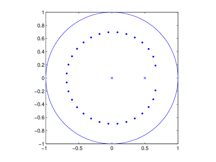
with $0<\rho<1$ . Observe that its inverse, $1/w$ , satisfies also the conditions of Theorem 2. However, the behavior of the zeros of the OPUC for $w$ and $1/w$ is qualitatively different, check Figure 2.

Refer to caption — Fig. 2: Zeros of $\Phi_{30}$ for weights $w$ (left) and $1/w$ (right), with $w$ given in (36) and $\rho=1/2$ .

In a few words, the explanation for this phenomenon is the following. Observe that in the case of an essential singularity of ${\mathcal{S}}$ the asymptotic behavior of the Cauchy transform

f_{n}^{(1)}(z)=-\frac{1}{2\pi i\tau^{2}}\,\oint_{{\mathbb{T}}_{r}}\frac{t^{n}{\mathcal{S}}(w;t)}{t-z}\,dt

is not as simple as when the only singular points are poles. In fact, the leading term of the asymptotics will come now from a dominant saddle point of

\displaystyle\Psi_{n}(t)

\displaystyle\stackrel{{\scriptstyle\text{\tiny def}}}{{=}}\log t+\frac{1}{n}\,\log{\mathcal{S}}(w;z)

lying close to the singular point of ${\mathcal{S}}$ , $t=t_{+}$ , which is the solution of the equation

\frac{1}{t}-\frac{1}{n+1}\,\left(\frac{t}{\rho t-1}+\frac{1}{t-\rho}\right)=0\quad\text{satisfying}\quad t_{+}=\rho+\sqrt{\frac{\rho}{n+1}}+\mathcal{O}\left(\frac{1}{n}\right)\,,\quad n\to\infty\,,

(37)

where we take the positive square root. It is possible to show that the zeros of the orthogonal polynomials (at least those not staying to close to $z=\rho$ ), will approach the level curve

\mathop{\rm Re}(\Psi_{n}(z)-\Psi_{n}(t_{+}))=\frac{1}{n}\,\log\left(\frac{1}{2\sqrt{\pi}}\frac{\rho^{3/4}}{n^{3/4}}\right)\,,

(38)

and the error decreases with $n$ . However, for the weight $1/w$ we will have two dominant saddle points, and the different structure of the level curve (38) for weights $w$ and $1/w$ explains the different result of the numerical experiments (see Figure (3)).

2.3 Verblunsky and leading coefficients

Let us finish this Section with some comments about the behavior of the notorious coefficients related to the OPUC.

Evaluating the polynomial $\Phi_{n+1}$ or any of its approximations at the origin we obtain information about the Verblunsky coefficients. For instance, a combination of (23), (27), and (29) yields the following estimate of the Verblunsky coefficients $\alpha_{n}$ :

Proposition 5 ([12]).

Let $w$ be a strictly positive analytic weight on the unit circle ${\mathbb{T}}_{1}$ . With the notation introduced above and for each $n\in\mathbb{N}$ ,

\alpha_{n}=-\left(\frac{1}{{\mathcal{S}}}\right)_{n+1}+\mathcal{O}(r^{3n})\,,

(39)

where $(1/{\mathcal{S}})_{n+1}$ is the corresponding Laurent coefficient of $1/{\mathcal{S}}$ in (25).

This fact has the following reading: consider the generating function of the Verblunsky coefficients,

G(z)=\sum_{n=0}^{\infty}\alpha_{n}z^{n}\,.

Then the Maclaurin series of $G$ and $\mathcal{P}_{+}(-z/{\mathcal{S}}(z))$ match up to the $\mathcal{O}(r^{3n})$ term. In consequence, we have

Proposition 6.

Function

G(z)+\frac{z}{{\mathcal{S}}(w;z)}\,,

defined in a neighborhood of ${\mathbb{T}}_{1}$ , can be continued as a holomorphic function to the annulus $1<|z|<1/\rho^{3}$ .

This fact has been established independently by Simon [17] and Deift and Östensson [6].

If the only singularities on ${\mathbb{T}}_{\rho}$ are dominant poles, we can use formula (34) in order to derive the asymptotic behavior of $\alpha_{n}$ ’s:

Proposition 7 ([12]).

Under assumptions of Theorem 4, the Verblunsky coefficients satisfy

\alpha_{n}=-\sum_{k=1}^{\ell}\binom{n+1}{m-1}\,\overline{a_{k}^{n-m+1}\,D_{\rm i}(w;a_{k})\,\widehat{D}_{\rm e}(w;a_{k})}+\begin{cases}\mathcal{O}\left(\rho^{n}\delta^{n}\right),&\text{if }\,m=1\,,\\ \mathcal{O}\left(n^{m-2}\,\rho^{n}\right)\,,&\text{if }\,m\geq 2\,.\end{cases}

That is, in the situation when the first singularities of $D_{\rm e}$ met during its analytic continuation inside are only poles, the Verblunsky coefficients are asymptotically equal to a combination of competing exponential functions with coefficients that are polynomials in $n$ . We can compare it with the case of the essential singularity considered before: for the weight $w$ given in (36),

\alpha_{n}=-\frac{1}{2\sqrt{\pi}}\,t_{+}^{n}{\mathcal{S}}(w;t_{+})\,\left(\frac{\rho}{n}\right)^{3/4}\left(1+\mathcal{O}\left(\frac{1}{n^{1/2}}\right)\right)\,,\quad n\to\infty\,,

where $t_{+}\to\rho$ is given by the equation (37).

A similar analysis can be carried out for the asymptotic expansion of the leading coefficients $\kappa_{n}$ . By (24),

\kappa_{n}^{2}=\frac{\tau^{2}}{2\pi}\,S_{22}(n+1;0)=\frac{\tau^{2}}{2\pi}\,\left(1+g_{n+1}^{(2)}(0)+\mathcal{O}(r^{4n})\right)\,.

Taking into account (28), we arrive at

Proposition 8.

For the leading coefficient $\kappa_{n}$ the following formula holds:

\kappa_{n}^{2}=\frac{\tau^{2}}{2\pi}\,\sum_{k>-n-1}|\left({\mathcal{S}}\right)_{k}|^{2}+\mathcal{O}(r^{4n})=\frac{\tau^{2}}{2\pi}\,\left(1-\sum_{k\leq-n-1}|\left({\mathcal{S}}\right)_{k}|^{2}\right)+\mathcal{O}(r^{4n})\,,

(40)

where $\left({\mathcal{S}}\right)_{k}$ ’s are the coefficients of the Laurent expansion of ${\mathcal{S}}$ in (25).

Observe that we can write this identity also in terms of the Riesz projections:

\kappa_{n}^{2}=\tau^{2}\left\|\mathcal{P}_{-}\left(\sigma_{n+1}^{-1}\right)\right\|^{2}_{L^{2}({\mathbb{T}}_{1},|dz|)}+\mathcal{O}(r^{4n})\,.

Formula (40) shows that

\lim_{n}\kappa_{n}^{2}=\frac{\tau^{2}}{2\pi}\,,\quad\text{and}\quad\kappa_{n+1}^{2}-\kappa_{n}^{2}=\frac{\tau^{2}}{2\pi}\,|({\mathcal{S}})_{-n-1}|^{2}+\mathcal{O}(r^{4n})\,,

in accordance with (39) and the well known fact that

\frac{1}{\kappa_{n+1}^{2}}-\frac{1}{\kappa_{n}^{2}}=-\frac{|\alpha_{n}|^{2}}{\kappa_{n}^{2}}.

Summarizing, we see that the Laurent coefficients of ${\mathcal{S}}$ (or of $1/{\mathcal{S}}$ ) contain surprisingly good approximations of two main parameters of the OPUC: they match asymptotically the Verblunsky coefficients, and the partial sums of the squares of their absolute values represent (up to a normalizing constant) the leading coefficient of the orthonormal polynomials.

3 Weight with zeros on ${\mathbb{T}}_{1}$

Let us analyze the change of the behavior of the orthogonal polynomials if we allow zeros of the weight on the unit circle. In other words, we consider now a weight of the form

W(z)\stackrel{{\scriptstyle\text{\tiny def}}}{{=}}w(z)\,\prod_{k=1}^{m}|z-a_{k}|^{2\beta_{k}}\,,\quad z\in{\mathbb{T}}_{1}\,,

(41)

where $a_{k}\in{\mathbb{T}}_{1}$ , $\beta_{k}\geq 0$ , $k=1,\dots,m$ , and $w$ is an analytic and positive weight on ${\mathbb{T}}_{1}$ , such as considered in Section 2. Without loss of generality we assume that $w$ is analytic and non-vanishing in the annulus $\rho<|z|<1/\rho$ .

According to Nevai and Totik [15], the Verblunsky coefficients no longer have an exponential decay, neither the bulk of zeros accumulate on an inner circle, but how many of them stay inside? And for those approaching the unit circle, does the rate depend on the “orders” $\beta_{k}$ ? And how can we extend the Riemann-Hilbert method, that so nicely worked for us in the analytic situation, to the case of a weight of the form (41)?

3.1 Steepest descent analysis

Matrix

Y(z)=\begin{pmatrix}\Phi_{n}(z)&\displaystyle\dfrac{1}{2\pi i}\,\oint_{{\mathbb{T}}_{1}}\dfrac{\Phi_{n}(t)W(t)\,dt}{t^{n}(t-z)}\\ -2\pi\kappa_{n-1}\varphi^{*}_{n-1}(z)&-\,\displaystyle\dfrac{\kappa_{n-1}}{i}\,\oint_{{\mathbb{T}}_{1}}\dfrac{\varphi^{*}_{n-1}(t)W(t)\,dt}{t^{n}(t-z)}\end{pmatrix}\,,

solves the Riemann-Hilbert problem (10), with $w$ replaced by $W$ . It is the unique solution if we add additional requirements at the zeros of the weight:

Y(z)=\mathcal{O}\begin{pmatrix}1&1\\ 1&1\end{pmatrix}\,,\quad\text{as }z\to a_{k},\;z\in\mathbb{C}\setminus{\mathbb{T}}_{1},\quad k=1,\dots,m.

Nothing hinders performing Step 1: with $H$ defined by (11) we put $T\stackrel{{\scriptstyle\text{\tiny def}}}{{=}}YH$ , so that $T$ becomes holomorphic in $\mathbb{C}\setminus{{\mathbb{T}}_{1}}$ (including the infinity) and

T_{+}(t)=T_{-}(t)\,\begin{pmatrix}t^{n}&W(t)\\ 0&t^{-n}\end{pmatrix}\,,\quad t\in{\mathbb{T}}_{1}\,.

However, in order to get rid of the oscillatory behavior of the diagonal entries of the jump matrix the lenses we opened in Step 2 of Section 2 are no longer valid, at least because $W$ has singularities on ${\mathbb{T}}_{1}$ . Since they are in a finite number, we can modify this step by opening lenses inside and outside ${\mathbb{T}}_{1}$ , but “attached” to the unit circle at $a_{k}$ ’s (see Figure 4).

\begin{overpic}[lenses2] \put(60.0,14.0){\small${\mathbb{T}}_{1}$} \put(36.0,32.0){$\gamma_{\rm i}$} \put(1.0,32.0){$\gamma_{\rm e}$} \put(45.0,65.0){$\Omega_{0}$} \put(69.0,69.0){$\Omega_{+}$} \put(81.0,76.0){$\Omega_{-}$} \put(100.0,70.0){$\Omega_{\infty}$} \put(22.0,68.0){\small$a_{m}$} \put(32.0,8.0){\small$a_{1}$} \put(90.0,31.0){\small$a_{2}$} \end{overpic}

Fig. 4: Opening lenses.

This deformation of the contour makes the definition of $K$ in (12) consistent (after replacing $w$ with $W$ ), in such a way that $U\stackrel{{\scriptstyle\text{\tiny def}}}{{=}}TK$ has the jumps

U_{+}(t)=U_{-}(t)\,J_{U}(t),\quad t\in{\gamma_{\rm i}}\cup{{\mathbb{T}}_{1}}\cup{\gamma_{\rm e}},

with

J_{U}(t)=\begin{cases}\begin{pmatrix}0&W(t)\\ -1/W(t)&0\end{pmatrix},&\text{if }t\in{{\mathbb{T}}_{1}},\\ \begin{pmatrix}1&0\\ t^{n}/W(t)&1\end{pmatrix},&\text{if }t\in{\gamma_{\rm i}},\\ \begin{pmatrix}1&0\\ 1/(t^{n}W(t))&1\end{pmatrix},&\text{if }t\in{\gamma_{\rm e}}.\end{cases}

(42)

Step 3: Our next goal is to handle the jump on ${\mathbb{T}}_{1}$ via the global parametrix $N$ built in Section 2 using the Szegő function. However, for $W$ as in (41) the Szegő function is, in general, no longer single-valued in the neighborhood of $a_{k}$ ’s, and a short digression is convenient in order to discuss briefly the form of this function and its multivaluedness.

For the sake of brevity we define the set of singularities of the weight, $\mathcal{A}\stackrel{{\scriptstyle\text{\tiny def}}}{{=}}\{a_{1},\dots,a_{m}\}$ . We fix for what follows $0<\delta<1-\rho$ , such that additionally $\delta<\frac{1}{3}\min_{i\neq j}|a_{i}-a_{j}|$ , so that all neighborhoods $B_{\delta}(a_{k})$ (see definition (32)) are disjoint. Denote also

c_{k}\stackrel{{\scriptstyle\text{\tiny def}}}{{=}}\{z\in\mathbb{C}:\,|z-a_{k}|=\delta\}\,,\quad k=1,\dots,m\,,

(43)

as well as $B\stackrel{{\scriptstyle\text{\tiny def}}}{{=}}\cup_{k=1}^{m}B_{\delta}(a_{k})$ . Furthermore, given a subset $X\subset\mathbb{C}$ and a value $a\in\mathbb{C}$ we will use the standard notation $a\cdot X=\{ax:\,x\in X\}$ ; consistently, ${\mathcal{A}}\cdot X\stackrel{{\scriptstyle\text{\tiny def}}}{{=}}\cup_{k=1}^{m}(a_{k}\cdot X)$ .

In order to construct explicitly the Szegő function for the modified weight $W$ we introduce the generalized polynomial

q(z)\stackrel{{\scriptstyle\text{\tiny def}}}{{=}}\prod_{k=1}^{m}(z-a_{k})^{\beta_{k}/2}

(44)

and select its single-valued analytic branch in $\mathbb{C}\setminus\left(\cup_{k=1}^{m}a_{k}\cdot[1,+\infty)\right)$ by fixing the value of $q(0)$ . With this convention we can write the Szegő functions for the modified weight $W$ :

D_{\rm i}(W;z)=\frac{q^{2}(z)}{q^{2}(0)}\,D_{\rm i}(w;z)\,,\quad D_{\rm e}(W;z)=\frac{D_{\rm e}(w;z)}{q^{2}(0)\,\overline{q(1/\bar{z})}^{2}}\,.

(45)

In particular, $D_{\rm i}(W;z)$ is holomorphic in $\mathbb{D}_{1/\rho}\setminus\left(\cup_{k=1}^{m}a_{k}\cdot[1,1/\rho)\right)$ , $D_{\rm e}(W;z)$ is holomorphic in $\{z\in\mathbb{C}:\,|z|>\rho\}\setminus\left(\cup_{k=1}^{m}a_{k}\cdot(\rho,1]\right)$ , and

\frac{1}{D_{\rm i}(W;0)}=\frac{1}{D_{\rm i}(w;0)}=D_{\rm e}(W;\infty)=D_{\rm e}(w;\infty)=\tau>0\,,

(46)

where $\tau$ has been defined in (13). Furthermore, with the orientation of the cuts toward infinity we have for $k=1,\dots,m$ :

\begin{split}\left[D_{\rm i}(W;z)\right]_{+}&=e^{-2\pi i\beta_{k}}\left[D_{\rm i}(W;z)\right]_{-}\,,\quad z\in a_{k}\cdot(1,1/\rho)\,,\\ \left[D_{\rm e}(W;z)\right]_{+}&=e^{-2\pi i\beta_{k}}\left[D_{\rm e}(W;z)\right]_{-}\,,\quad z\in a_{k}\cdot(\rho,1)\,.\end{split}

(47)

By definition (6) and formulas (45) we have

{\mathcal{S}}(W;z)=D_{\rm i}(W;z)D_{\rm e}(W;z)=\left(\frac{q(z)}{q^{2}(0)\,\overline{q(1/\bar{z})}}\right)^{2}{\mathcal{S}}(w;z)\,,

that is also analytic and single-valued in the cut annulus $\{\rho<|z|<1/\rho\}\setminus\left({\mathcal{A}}\cdot(\rho,1/\rho)\right)$ ; furthermore, with our assumptions on $\delta$ , function

\widehat{\mathcal{S}}_{k}(W;z)\stackrel{{\scriptstyle\text{\tiny def}}}{{=}}\begin{cases}e^{\pi i\beta_{k}}{\mathcal{S}}(W;z)\,,&\text{if }z\in B_{\delta}(a_{k})\text{ and }\arg(z)>\arg(a_{k})\,,\\ e^{-\pi i\beta_{k}}{\mathcal{S}}(W;z)\,,&\text{if }z\in B_{\delta}(a_{k})\text{ and }\arg(z)<\arg(a_{k})\,,\end{cases}

(48)

is holomorphic in $B_{\delta}(a_{k})$ , $k=1,\dots,m$ . So, we can define

\vartheta_{k}\stackrel{{\scriptstyle\text{\tiny def}}}{{=}}\widehat{\mathcal{S}}_{k}(W;a_{k})\in{\mathbb{T}}\,,\quad k=1,\dots,m\,.

(49)

Now let us get back to the global parametrix $N(z)=N(W;z)$ , given by formula (15), that is well defined, has the same jumps on ${\mathbb{T}}_{1}$ as $U(z)$ , and by (46), it exhibits the same behavior at infinity. Hence, $U(z)N^{-1}(z)$ tends to $I$ as $z\to\infty$ , and is holomorphic in $\mathbb{C}\setminus(\gamma_{\rm e}\cup\gamma_{\rm i})$ . The jump on these curves is again exponentially close to identity, except in a neighborhood of the zeros $a_{k}$ of the weight $W$ . This is a new feature, and we have to deal with this problem separately.

Step 4: local analysis. Let us pick a singular point $a_{k}\in{\mathcal{A}}$ . For the sake of brevity along this subsection we use the following shortcuts for the notation: $a\stackrel{{\scriptstyle\text{\tiny def}}}{{=}}a_{k}$ , $\beta\stackrel{{\scriptstyle\text{\tiny def}}}{{=}}\beta_{k}$ , $b\stackrel{{\scriptstyle\text{\tiny def}}}{{=}}B_{\delta}(a_{k})$ , $c\stackrel{{\scriptstyle\text{\tiny def}}}{{=}}c_{k}$ (where $c_{k}$ were defined in (43)), and $b^{+}\stackrel{{\scriptstyle\text{\tiny def}}}{{=}}\{z\in b:\,\arg(z)>\arg(a)\}$ , $b^{-}\stackrel{{\scriptstyle\text{\tiny def}}}{{=}}\{z\in b:\,\arg(z)<\arg(a)\}$ . We also write $\widehat{\Omega}_{j}\stackrel{{\scriptstyle\text{\tiny def}}}{{=}}\Omega_{j}\cap b$ , where $j\in\{{\rm i},{\rm e},0,\infty\}$ , and analogous notation for curves: $\widehat{\mathbb{T}}_{1}\stackrel{{\scriptstyle\text{\tiny def}}}{{=}}{\mathbb{T}}_{1}\cap b$ , etc.

The goal is to build a matrix $P$ such that it is holomorphic in $b\setminus({\mathbb{T}}_{1}\cup\gamma_{\rm i}\cup\gamma_{\rm e})$ , satisfies across $\widehat{\mathbb{T}}_{1}\cup\widehat{\gamma}_{\rm i}\cup\widehat{\gamma}_{\rm e}$ the jump relation $P_{+}=P_{-}J_{U}$ , with $J_{U}$ given in (42), with the same local behavior as $U$ close to $z=a$ , and matching $N$ on $c$ . This analysis is very technical, and we refer the reader to [11] for details, and describe here the main ideas in a very informal fashion.

\begin{overpic}[lenses_new2] \put(50.0,30.0){$\gamma_{\rm i}$} \put(20.0,50.0){$\gamma_{\rm i}$} \put(48.0,75.0){$\gamma_{\rm e}$} \put(85.0,45.0){$\gamma_{\rm e}$} \put(40.0,20.0){$\Omega_{0}$} \put(20.0,40.0){$\Omega_{0}$} \put(65.0,85.0){$\Omega_{\infty}$} \put(80.0,65.0){$\Omega_{\infty}$} \put(35.0,85.0){$\Omega_{\rm e}$} \put(85.0,35.0){$\Omega_{\rm e}$} \put(12.0,62.0){$\Omega_{\rm i}$} \put(70.0,15.0){$\Omega_{\rm i}$} \put(17.0,25.0){$\Gamma_{\rm i}$} \put(80.0,75.0){$\Gamma_{\rm e}$} \put(49.0,47.0){\small$a$} \put(15.0,73.0){\small${\mathbb{T}}_{1}$} \end{overpic}

Fig. 5: Local analysis in

b

As a first step we reduce the problem to the one with constant jumps. Let us denote $\Gamma_{\rm i}\stackrel{{\scriptstyle\text{\tiny def}}}{{=}}a\cdot(1-\delta,1)$ and $\Gamma_{\rm e}\stackrel{{\scriptstyle\text{\tiny def}}}{{=}}a\cdot(1,1+\delta)$ , oriented both from $z=a$ to infinity (see Fig. 5). Let $w^{1/2}(z)$ and $z^{1/2}$ denote the principal holomorphic branches of these functions in $b$ , and $W^{1/2}(z)\stackrel{{\scriptstyle\text{\tiny def}}}{{=}}q(z)\overline{q(1/\overline{z})}\,w^{1/2}(z)$ , with $q$ defined in (44). Then $W^{1/2}$ is holomorphic in $b\setminus a\cdot(1-\delta,1+\delta)$ , and according to (47),

\frac{W^{1/2}_{+}(z)}{W^{1/2}_{-}(z)}=e^{-\pi i\beta}\quad\text{on }\Gamma_{\rm i}\,,\quad\text{and}\quad\frac{W^{1/2}_{+}(z)}{W^{1/2}_{-}(z)}=e^{\pi i\beta}\quad\text{on }\Gamma_{\rm e}\,.

Thus, if we define

\lambda(\beta;z)\stackrel{{\scriptstyle\text{\tiny def}}}{{=}}\begin{cases}e^{\pi i\beta}W^{1/2}(z)z^{n/2},&z\in(\widehat{\Omega}_{\rm e}\cup\widehat{\Omega}_{\infty})\cap b^{+},\\ e^{-\pi i\beta}W^{1/2}(z)z^{n/2},&z\in(\widehat{\Omega}_{\rm e}\cup\widehat{\Omega}_{\infty})\cap b^{-},\\ e^{-\pi i\beta}W^{1/2}(z)z^{-n/2},&z\in(\widehat{\Omega}_{\rm i}\cup\widehat{\Omega}_{0})\cap b^{+},\\ e^{\pi i\beta}W^{1/2}(z)z^{-n/2},&z\in(\widehat{\Omega}_{\rm i}\cup\widehat{\Omega}_{0})\cap b^{-},\end{cases}\,,

(50)

and set

R(z)\stackrel{{\scriptstyle\text{\tiny def}}}{{=}}P(z)\,\lambda(\beta;z)^{\sigma_{3}}\,,\quad z\in b\setminus(\Gamma_{\rm i}\cup\Gamma_{\rm e}\cup{\mathbb{T}}_{1}\cup\gamma_{\rm i}\cup\gamma_{\rm e})\,,

(51)

we get for $R$ the following problem: $R$ is holomorphic in $b\setminus(\Gamma_{\rm i}\cup\Gamma_{\rm e}\cup{\mathbb{T}}_{!}\cup\gamma_{\rm i}\cup\gamma_{\rm e})$ , and satisfies the jump relation $R_{+}(z)=R_{-}(z)J_{R}(z)$ , with

J_{R}(z)=\begin{cases}\begin{pmatrix}0&1\\ -1&0\end{pmatrix},&\text{if }z\in\widehat{\mathbb{T}}_{1},\\ \begin{pmatrix}1&0\\ e^{-2\pi i\beta}&1\end{pmatrix},&\text{if }z\in(\widehat{\gamma}_{\rm i}\cap b^{+})\cup(\widehat{\gamma}_{\rm e}\cap b^{-}),\\ \begin{pmatrix}1&0\\ e^{2\pi i\beta}&1\end{pmatrix},&\text{if }z\in(\widehat{\gamma}_{\rm i}\cap b^{-})\cup(\widehat{\gamma}_{\rm e}\cap b^{+}),\\ \begin{pmatrix}e^{\pi i\beta}&0\\ 0&e^{-\pi i\beta}\end{pmatrix},&\text{if }z\in\Gamma_{\rm i}\cup\Gamma_{\rm e}\,.\end{cases}

Moreover, $R$ has the following local behavior as $z\to a$ :

R(z)=\begin{cases}\mathcal{O}\begin{pmatrix}|z-a|^{\beta}&|z-a|^{-\beta}\\ |z-a|^{\beta}&|z-a|^{-\beta}\end{pmatrix},&\text{if }z\in\widehat{\Omega}_{0}\cup\widehat{\Omega}_{\infty},\\ \mathcal{O}\begin{pmatrix}|z-a|^{-\beta}&|z-a|^{-\beta}\\ |z-a|^{-\beta}&|z-a|^{-\beta}\end{pmatrix},&\text{if }z\in\widehat{\Omega}_{\rm e}\cup\widehat{\Omega}_{\rm i}.\end{cases}

Consider in $\mathbb{C}\setminus(-\infty,0)$ the transformation

\zeta=-i\,\frac{n}{2}\,\log(z/a)\,,

(52)

(we omit the explicit reference to the dependence of $\zeta$ from $a$ and $n$ in the notation), where we take the main branch of the logarithm. This is a conformal 1-1 map of $b$ onto a neighborhood of the origin. Moreover, ${\mathbb{T}}_{1}$ is mapped onto $\mathbb{R}$ oriented positively, $\Gamma_{\rm i}\cup\Gamma_{\rm e}$ are mapped on the imaginary axis, and we may use the freedom in the selection of the contours deforming them in such a way that $f(\widehat{\gamma}_{\rm i})$ and $f(\widehat{\gamma}_{\rm e})$ follow the rays $\{\arg\zeta=\pm\frac{\pi}{4}\pm\pi\}$ . After this transformation we get a Riemann-Hilbert problem on the $\zeta$ -plane that has been studied for the local analysis of the generalized Jacobi weight on the real line. We take advantage of the results proved therein in order to abbreviate the exposition, and refer the reader to [20, Theorem 4.2] where the solution $\Psi\left(\beta;\zeta\right)$ is explicitly written in terms of the Hankel and modified Bessel functions.

Since a left multiplication by a holomorphic function has no influence on the jumps, and taking into account (51), we see that matrix $P$ can be built of the form

P(z)=E(z)\,\Psi\left(\beta;\zeta\right)\,\lambda(\beta;z)^{-\sigma_{3}}\,,

(53)

where $E$ is any holomorphic function in $b$ . An adequate selection of $E$ is motivated by the matching requirement $P(z)N^{-1}(z)=I+\mathcal{O}(n^{-1})$ on the boundary $c$ , and is constructed analyzing the asymptotic behavior of the matrix-valued function $\Psi\left(\beta;\zeta\right)$ at infinity. Let us summarize the results of this analysis:

Proposition 9.

Let

E(z)\stackrel{{\scriptstyle\text{\tiny def}}}{{=}}\left(\frac{\widehat{S}_{k}(W;z)}{\tau^{2}}\,ia^{n}\right)^{\sigma_{3}/2}\frac{1}{\sqrt{2}}\,\begin{pmatrix}i&1\\ -1&-i\end{pmatrix}\,,

(54)

where $\widehat{S}_{k}(W;\cdot)$ has been defined in (48), and we take the main branch of the square root. Then matrix $P(z)=P(a,\beta;z)$ ,

P(a,\beta;z)\stackrel{{\scriptstyle\text{\tiny def}}}{{=}}E(z)\,\Psi\left(\beta;\zeta\right)\,\lambda(\beta;z)^{-\sigma_{3}}\,,

(55)

with $\zeta$ given by (52), satisfies:

(i)

$U(z)P^{-1}(z)$ is holomorphic in $b$ ;

(ii)

for $z\in c$ ,

\begin{split}P(z)N^{-1}(z)=&I+\frac{i\beta}{2\zeta}\,\begin{pmatrix}\beta&-\tau^{-2}a^{n}\widehat{\mathcal{S}}(W;z)\\[8.61108pt] \tau^{2}a^{-n}\widehat{\mathcal{S}}^{-1}(W;z)&-\beta\end{pmatrix}+\mathcal{O}\left(\frac{1}{n^{2}}\right)\,.\end{split}

(56)

In particular, $P(z)N^{-1}(z)=I+\mathcal{O}(n^{-1})$ for $z\in c$ .

Step 5: asymptotic analysis. With the notation introduced in (43) and with $P(a,\beta;z)$ defined by (54)–(55) let us take

P(z)\stackrel{{\scriptstyle\text{\tiny def}}}{{=}}P(a_{k},\beta_{k};z)\quad\text{for }z\in B_{\delta}(a_{k})\setminus({\mathbb{T}}_{1}\cup\gamma_{\rm e}\cup\gamma_{\rm i}),\quad k=1,\dots,m\,,

and put

S(z)\stackrel{{\scriptstyle\text{\tiny def}}}{{=}}\begin{cases}U(z)N^{-1}(z),&\text{for }z\in\mathbb{C}\setminus(B\cup{\mathbb{T}}_{1}\cup\gamma_{\rm e}\cup\gamma_{\rm i}),\\ U(z)P^{-1}(z),&\text{for }z\in B\setminus({\mathbb{T}}_{1}\cup\gamma_{\rm e}\cup\gamma_{\rm i}).\end{cases}

\begin{overpic}[lensesFinal2] \put(35.0,45.0){$\gamma_{\rm i}$} \put(7.0,39.0){$\gamma_{\rm e}$} \put(11.0,75.0){\small$c_{m}$} \put(32.0,19.0){\small$c_{1}$} \put(82.0,41.0){\small$c_{2}$} \end{overpic}

Fig. 6: Jumps of

S

Matrix $S$ is holomorphic in the whole plane cut along $\gamma\cup C$ , where

\gamma\stackrel{{\scriptstyle\text{\tiny def}}}{{=}}(\gamma_{\rm e}\cup\gamma_{\rm i})\setminus B\quad\text{and}\quad C\stackrel{{\scriptstyle\text{\tiny def}}}{{=}}\cup_{k=1}^{m}c_{k}

(see Fig. 6), $S(z)\to I$ as $z\to\infty$ , and if we orient all $c_{k}$ ’s clockwise, $S_{+}(t)=S_{-}(t)J_{S}$ , with

J_{S}(t)=\begin{cases}P(z)N^{-1}(z),&\text{if }z\in C,\\ \begin{pmatrix}1&0\\ \tau^{2}/(z^{n}{\mathcal{S}}(W;z))&1\end{pmatrix},&\text{if }z\in\gamma_{\rm e}\setminus B,\\ \begin{pmatrix}1&-z^{n}{\mathcal{S}}(W;z)/\tau^{2}\\ 0&1\end{pmatrix},&\text{if }z\in\gamma_{\rm i}\setminus B.\\ \end{cases}

It is clear that the off-diagonal terms of $J_{S}$ on $\gamma_{\rm i}\setminus B$ and $\gamma_{\rm e}\setminus B$ decay exponentially fast. On the other hand, by (56), $J_{S}(z)=I+\mathcal{O}(1/n)$ for $z\in C$ . So the conclusion is that the jump matrix $J_{S}=I+O(1/n)$ uniformly for $z\in\gamma\cup C$ . Then arguments such as in [7, 4, 5] lead to the following conclusion:

Proposition 10.

Matrix $S$ satisfies the following singular integral equation:

S(z)=I+\frac{1}{2\pi i}\,\int\frac{(J_{S}(t)-I)\,dt}{t-z}+\frac{1}{2\pi i}\,\int\frac{(S_{-}(t)-I)(J_{S}(t)-I)\,dt}{t-z}\,,

where we integrate along contours $\gamma\cup C$ with the orientation shown in Fig. 6. In particular, integrating counter-clockwise,

S(z)=I-\sum_{k=1}^{m}\frac{1}{2\pi i}\,\oint_{c_{k}}\frac{(P(t)N^{-1}(t)-I)\,dt}{t-z}+O\left(\frac{1}{n^{2}}\right)

locally uniformly for $z\in\mathbb{C}\setminus(\gamma\cup C).$

Now formula (56) and the residue theorem yield for $z\in\mathbb{C}\setminus(\gamma\cup B)$ ,

S(z)=I+\frac{1}{n}\,\sum_{k=1}^{m}\dfrac{a_{k}\beta_{k}}{a_{k}-z}\,\begin{pmatrix}\beta_{k}&-\tau^{-2}a_{k}^{n}\vartheta_{k}\\[8.61108pt] \tau^{2}a_{k}^{-n}\vartheta_{k}^{-1}&-\beta_{k}\end{pmatrix}+O\left(\frac{1}{n^{2}}\right)\,.

(57)

We are ready for the asymptotic analysis of the original matrix $Y$ (and in particular, of its entries $(1,1)$ and $(2,1)$ ).

Unraveling our transformations we have

Y(z)=\begin{cases}S(z)N(z)K^{-1}(z)\,H^{-1}(z),&\text{if }z\in\mathbb{C}\setminus B,\\ S(z)P(z)K^{-1}(z)\,H^{-1}(z),&\text{if }z\in B.\end{cases}

We must analyze the consequences of these formulas in each domain (see Fig. 7).

\begin{overpic}[lensesFinal] \put(55.0,27.0){\small${\mathbb{T}}_{1}$} \put(35.0,45.0){$\gamma_{\rm i}$} \put(7.0,39.0){$\gamma_{\rm e}$} \put(40.0,65.0){$\Omega_{0}$} \put(65.0,69.0){$\Omega_{\rm i}$} \put(74.0,75.0){$\Omega_{\rm e}$} \put(87.0,82.0){$\Omega_{\infty}$} \put(11.0,75.0){\small$c_{m}$} \put(32.0,19.0){\small$c_{1}$} \put(82.0,41.0){\small$c_{2}$} \end{overpic}

Fig. 7: Domains for the asymptotic analysis.

We will do it only for the interior domain $\Omega_{0}\setminus B$ , where

N(z)=\begin{pmatrix}0&D_{\rm i}(W;z)/\tau\\ -\tau/D_{\rm i}(W;z)&0\end{pmatrix},\quad K(z)=H(z)=I\,.

Hence, $Y(z)=S(z)N(z)$ , so that

Y_{11}(z)=-\frac{\tau}{D_{\rm i}(W;z)}\,S_{12}(z)\,,\quad Y_{21}(z)=-\frac{\tau}{D_{\rm i}(W;z)}\,S_{22}(z)\,.

Taking into account (46) and (57), and recalling that $\Phi_{n}=Y_{11}$ we obtain

\Phi_{n}(z)=\frac{D_{\rm i}(W;0)}{D_{\rm i}(W;z)}\,\frac{1}{n}\,\left(\sum_{k=1}^{m}\dfrac{\beta_{k}\vartheta_{k}}{a_{k}-z}\,a_{k}^{n+1}+O\left(\frac{1}{n}\right)\right)\,,

valid uniformly in this domains. It shows in particular that for every compact set $K\subset\mathbb{D}_{1}$ there exists $N=N(K)\in\mathbb{N}$ such that for every $n\geq N$ , each $\Phi_{n}$ has at most $m-1$ zeros on $K$ , and these zeros should be asymptotically close to those of the rational fraction

\sum_{k=1}^{m}\dfrac{\beta_{k}\vartheta_{k}}{a_{k}-z}\,a_{k}^{n+1}\,.

(58)

Evaluating $\Phi_{n}(z)$ at $z=0$ we can obtain asymptotics for the Verblunsky coefficients $\alpha_{n}$ ; I leave this as an exercise for an interested reader.

Remark: Orthogonal polynomials with respect to non-analytic (but smooth) and non-vanishing weights with finite jump discontinuities on ${\mathbb{T}}_{1}$ were studied in [13], using a different (but complementary) method based on the $\overline{\partial}$ problem. There are very interesting similarities with our case: roughly speaking, both zeros and jump discontinuities of the weight have the same effect on the asymptotics of $\Phi_{n}$ ’s inside the unit disk $\mathbb{D}_{1}$ . More precisely, according to [13], if $W>0$ is sufficiently smooth and piecewise continuous, with jump discontinuities at $a_{k}\in{\mathbb{T}}_{1}$ , $k=1,\dots,m$ , then with a proper normalization, $\Phi_{n}(z)$ for $z$ on compact subsets of $\mathbb{D}_{1}$ will be asymptotically close to rational fractions of the form (58), with the basic difference that now coefficients $\beta_{k}$ stand for the magnitude of the jump of $\log W$ at $a_{k}$ (cf. formula (56) in [13] and the fact that for the scattering function on ${\mathbb{T}}_{1}$ ,

\mathcal{S}\left(W;e^{i\theta}\right)=e^{\Omega(\theta)}\,,

where $\Omega$ is defined by (21) in [13]). These similarities have as a common ground the duality of both cases: for $W$ in (41), the imaginary part of $\log W$ has jumps proportional to $\beta_{k}$ ’s, while in [13] the finite jumps correspond to $\mathop{\rm Re}\left(\log W\right)$ .

Finally, recall that the leading coefficient $\kappa_{n}$ of the orthonormal polynomial $\varphi_{n}$ is expressed in terms of $Y$ by $Y_{21}(0)=-2\pi\kappa_{n-1}^{2}$ . This yields immediately the following asymptotic formula:

\kappa_{n-1}^{2}=\frac{\tau^{2}}{2\pi}\,\left(1-\frac{1}{n}\,\sum_{k=1}^{m}\beta_{k}^{2}+\mathcal{O}\left(\frac{1}{n^{2}}\right)\right)\,,\quad n\to\infty.

This result has a consequence for the behavior of the Toeplitz determinants for $W$ . If we define the moments

d_{k}\stackrel{{\scriptstyle\text{\tiny def}}}{{=}}\oint_{z\in{\mathbb{T}}}z^{-n}W(z)|dz|\,,

then the Toeplitz determinants are

\mathcal{D}_{n}(W)\stackrel{{\scriptstyle\text{\tiny def}}}{{=}}\det\left[\left(d_{j-i}\right)_{i,j=0}^{n}\right]\,.

(59)

It is known (see e.g. [18, Theorem 1.5.11]) that

\frac{\mathcal{D}_{n}(W)}{\mathcal{D}_{n-1}(W)}=\frac{1}{\kappa_{n}^{2}}\,.

Taking into account the asymptotics of $\kappa_{n}$ , (14) and (46), we arrive at

Theorem 11.

Under the assumption above there exists a constant $\varkappa$ depending on $W$ such that

\begin{split}\mathcal{D}_{n}(W)&=\varkappa\,\left(G[2\pi w]\right)^{n}\,n^{\sum_{k=1}^{m}\beta_{k}^{2}}\,\left(1+o(1)\right)\,,\quad n\to\infty\,.\end{split}

(60)

This formula is in accordance with the well known Fisher-Hartwig conjecture (see e.g. [2]), proved for this case (but using totally different approach and giving an expression for $\varkappa$ ) by Widom in [21].

Acknowledgements

The research of this author was supported, in part, by a grant from the Ministry of Education and Science of Spain, project code MTM2005-08648-C02-01, by Junta de Andalucía, Grupo de Investigación FQM229, by “Research Network on Constructive Complex Approximation (NeCCA)”, INTAS 03-51-6637, and by NATO Collaborative Linkage Grant “Orthogonal Polynomials: Theory, Applications and Generalizations”, ref. PST.CLG.979738.

I wish to acknowledge also the contribution of both anonymous referees, whose careful reading of the manuscript and kind suggestions helped to improve the text.

A vast portion of the results exposed here is an outcome of a highly enjoyable collaboration with K. T.-R. McLaughlin, from the University of Arizona, USA, and with E. B. Saff, from the Vanderbilt University, USA. In particular, this celebration is a good occasion to express once again my gratitude to Ed Saff for his support and friendship.

References

[1] J. Baik, P. Deift, and K. Johansson. On the distribution of the length of the longest increasing subsequence of random permutations. J. Amer. Math. Soc., 12(4):1119–1178, 1999.
[2] E. L. Basor and C. A. Tracy. The Fisher-Hartwig conjecture and generalizations. Physica A, 177:167–173, 1991.
[3] P. Deift. Integrable operators. In Differential Operators and Spectral Theory, pages 69–84. Amer. Math. Soc., Providence, RI, 1999. Amer. Math. Soc. Transl. Ser. 2, 189,.
[4] P. Deift, T. Kriecherbauer, K. T-R McLaughlin, S. Venakides, and X. Zhou. Strong asymptotics of orthogonal polynomials with respect to exponential weights. Comm. Pure Appl. Math., 52(12):1491–1552, 1999.
[5] P. Deift, T. Kriecherbauer, K. T.-R. McLaughlin, S. Venakides, and X. Zhou. Uniform asymptotics for polynomials orthogonal with respect to varying exponential weights and applications to universality questions in random matrix theory. Comm. Pure Appl. Math., 52(11):1335–1425, 1999.
[6] P. Deift and J. Östensson. A Riemann-Hilbert approach to some theorems on Toeplitz operators and orthogonal polynomials. Arxiv:math.FA/0504284.
[7] P. A. Deift. Orthogonal polynomials and random matrices: a Riemann-Hilbert approach. New York University Courant Institute of Mathematical Sciences, New York, 1999.
[8] A.S. Fokas, A.R. Its, and A.V. Kitaev. The isomonodromy approach to matrix models in 2D quantum gravity. Comm. Math. Phys., 147:395–430, 1992.
[9] J. S. Geronimo and K. M. Case. Scattering theory and polynomials orthogonal on the unit circle. J. Math. Phys., 20(2):299–310, 1979.
[10] A. B. J. Kuijlaars. Riemann-Hilbert Analysis for Orthogonal Polynomials. In “Orthogonal Polynomials and Special Functions: Leuven 2002”, Lecture Notes Math., 1817:167–210, 2003.
[11] A. Martínez-Finkelshtein, K. T.-R. McLaughlin, and E. B. Saff. Asymptotics of orthogonal polynomials with respect to a weight with zeros on the circle. Preprint in preparation, 2006.
[12] A. Martínez-Finkelshtein, K. T.-R. McLaughlin, and E. B. Saff. Szegő orthogonal polynomials with respect to an analytic weight: canonical representation and strong asymptotics. Constr. Approx., 2006. in press. Also preprint arXiv:math.CA/0502300.
[13] K. T.-R. McLaughlin and P. D. Miller. The $\overline{\partial}$ steepest descent method and the asymptotic behavior of polynomials orthogonal on the unit circle with fixed and exponentially varying nonanalytic weights. Preprint arXiv:math.CA/0406484, 2004.
[14] H.N. Mhaskar and E. B. Saff. On the distribution of zeros of polynomials orthogonal on the unit circle. J. Approx. Theory, 63:30–38, 1990.
[15] P. Nevai and V. Totik. Orthogonal polynomials and their zeros. Acta Sci. Math. (Szeged), 53(1-2):99–104, 1989.
[16] B. Simon. Fine structure of the zeros of orthogonal polynomials, I. A tale of two pictures. preprint, 2004.
[17] B. Simon. Meromorhic Szegő functions and asymptotic series for Verblunsky coefficients. To appear in Acta Math. Also preprint Arxiv:math SP/0502489.
[18] B. Simon. Orthogonal Polynomials on the Unit Circle I and II, volume 54 of AMS Colloquium Publications. American Mathematical Society, Providence, RI, 2005.
[19] G. Szegő. Orthogonal Polynomials, volume 23 of Amer. Math. Soc. Colloq. Publ. Amer. Math. Soc., Providence, RI, fourth edition, 1975.
[20] M. Vanlessen. Strong asymptotics of the recurrence coefficients of orthogonal polynomials associated to the generalized Jacobi weight. J. Approx. Theory, 125:198–237, 2003.
[21] H. Widom. Toeplitz determinants with singular generating functions. Amer. J. Math., 95:333–383, 1973.

Szegő polynomials: a view from the Riemann-Hilbert windowThanks: This paper is dedicated to Ed Saff on the occasion of his 60th birthday.

Abstract

keywords

AMS

1 Introduction

2 Analytic and nonvanishing weight

2.1 Steepest descent analysis and canonical representation for orthogonal polynomials

Theorem 1.

2.2 Asymptotic behavior of OPUC

Theorem 2 ([12]).

Definition 3.

Theorem 4 ([12]).

2.3 Verblunsky and leading coefficients

Proposition 5 ([12]).

Proposition 6.

Proposition 7 ([12]).

Proposition 8.

3 Weight with zeros on 𝕋1{\mathbb{T}}_{1}

3.1 Steepest descent analysis

Proposition 9.

Proposition 10.

Theorem 11.

Acknowledgements

References

3 Weight with zeros on ${\mathbb{T}}_{1}$