Orbit structure for groups of homeomorphisms of
Abstract
In this paper we will refine Sacksteder’s theorem for groups of orientation-preserving homeomorphisms of the circle in the case that there exists a finite orbit set. We will give a categorization of the topological possibilities for the orbits of points of the circle, along with examples.
1 Introduction
In this paper we consider groups of orientation-preserving homeomorphisms of the circle, acting in the natural way, and give a complete categorization of the topological possibilities for orbits of points of the circle under the action of the group. This is an extension of Sacksteder’s theorem ([2], p. 20), which gives three possible orbit types, but does not describe the remaining possibilities. In particular, if there is a finite orbit set, it does not describe the structure of the remaining orbits.
In Section 2 we will review the Poincaré classification of orbits for circle homeomorphisms, and recall Sacksteder’s theorem for groups of homeomorphisms. The intent of this paper is to refine Sacksteder’s theorem in the case that the action of the group has a finite orbit.
In Section 3 we will prove the following:
Lemma 1.
Let be a group of orientation-preserving homeomorphisms of the interval and suppose satisfies one of the following conditions:
- 1.
is finitely generated and there are no fixed points of the group in .
- 2.
There exists at least one group element of whose fixed points do not accumulate at either 0 or 1.
Then every nonempty -invariant set that is closed with respect to contains a nonempty, -invariant set closed in and minimal under those properties.
We will assume throughout the rest of the paper that the group of orientation-preserving homeomorphisms of the circle has a finite number of finite orbit points, which we denote . We will split the circle at points of and look at the complementary subintervals, which we call . If the finite orbits points in are all fixed under the group, then the orbit of any point will be entirely contained in one ; if not, it will be contained in the union of some number of the . We call the union of the intervals which the orbit of intersects nontrivially , for range of . We assume the group , restricted to one , satisfies one of the conditions of the lemma. We then prove the following:
Theorem 1.
For all , there are four possibilities for the orbit of :
- 1.
is dense in .
- 2.
accumulates exactly at points of .
- 3.
is contained in a -invariant Cantor set in . The orbit of is dense in the Cantor set, and the Cantor set is contained in the closure of the orbit of each point of .
- 4.
contains a proper subset which is -invariant, closed with respect to , and which does not intersect ; i.e., accumulates at the closure of another orbit.
In Section 4 we will give a collection of examples to demonstrate the four cases of the theorem. In particular, we will give two different examples that have a Cantor set, and we will look at several examples designed to explore the different topological possibilites of a point in Case 4. This will lead us to define the level of an orbit (see 4.8), so that we can describe the nesting of orbits that may occur in this case.
In Section 5 we will consider semigroups rather than groups, and give an example which demonstrates one way in which the orbit type under a semigroup can differ from those for groups.
Section 6 is devoted to a closer examination of Case 4, the case in the theorem that admits the most complexity of orbits. We will prove a collection of lemmas whose purpose is to reduce the number of considerations necessary to understand the range of possibilities, and we will define a few of the special orbit types that may arise.
In Section 7 we will prove results for points in the fourth case when the group homeomorphisms are analytic.
Finally, in Section 8 we will conclude with some conjectures for future work.
2 Preliminaries
The classical theory of dynamical systems studies the orbit structure of a homeomorphism or a flow on a manifold, in particular, the topological properties of or . This corresponds to studying actions of the group or . One can ask under what circumstances a map will have periodic points, dense orbits, etc. One can also study the actions of more general groups. In this paper we will look at the orbit structure of a group of homeomorphisms acting in a natural way on the circle.
Poincaré classified the possible behavior of orbits for a given homeomorphism of the circle by looking at the rotation number of the homeomorphism, an invariant that gives the “average” rotation under the map. For a more thourough discussion of these concepts, see [3], Chapter 11. He showed that points of can have six different kinds of orbits under homeomorphisms: three types each for rational and irrational rotation numbers. The possibilities are: a periodic orbit, a homoclinic orbit approaching a given periodic orbit, a heteroclinic orbit approaching two different periodic orbits, a dense orbit, an orbit dense in a Cantor set, and an orbit homoclinic to a Cantor set.
When studying the action of a group of homeomorphisms, we discuss the group orbit of a point , denoted . We often refer to this as the orbit of the point without making reference to the group. This is not to be confused with the orbit of a point under a single map (generally a “smaller” set). Sacksteder’s theorem describes the main possibilities for the dynamics of an arbitrary group of homeomorphisms. See [2] for a discussion and proof.
Theorem 2 (Sacksteder).
Let be any subgroup of , the orientation-preserving homeomorphisms of the circle. There are three mutually exclusive possibilities:
- 1.
There is a finite orbit.
- 2.
All orbits are dense.
- 3.
There is a compact -invariant subset which is infinite and different from and such that the orbits of points in are dense in . This set is unique, contained in the closure of any orbit, and is homeomorphic to a Cantor set.
The three options are directly related to the types of invariant minimal sets which can exist for homeomorphisms of the circle. It is known that the circle supports three different types of invariant minimal sets under the action of a homeomorphism: finite sets, Cantor sets, and the circle itself. As the orbit of a point under a homeomorphism is automatically invariant under that map, it is easy to see how the results of the classification theorems reflect those options. Unsurprisingly, the proof of this theorem relies heavily on the ability to find a minimal set which is compact and invariant under the action of the group. We are interested in extending the result when there is a known finite orbit, in order to understand the behavior of all the nonfinite orbits in this case. We will also need to find a minimal set; however, it will take some extra work.
3 Groups of Homeomorphisms
Unless indicated otherwise, throughout the rest of this paper we shall assume the following:
- 1.
acts on the circle in the natural way, i.e., for all , .
- 2.
The action of on the circle has a (nonzero) finite number of finite orbits. Denote by be the set of points of finite orbits.
- 3.
is either finitely generated, or has at least one group element with isolated fixed points.
Notationally, we will use to be the open unit interval, and to be the closed.
Definition 1.
If a set is invariant under the action of the group and closed with respect to a proper subset , we will say that is a -set. If contains no proper subset that is also -invariant and closed in , we will say that is -minimal.
We use the following lemma repeatedly:
Lemma 2.
Let be a group of orientation-preserving homeomorphisms of . Suppose either of the following conditions are satisfied:
- C1
There exists at least one group element whose fixed points do not accumulate at 0 and do not accumulate at 1.
- C2
G is finitely generated and there are no fixed points of the group in .
Then each nonempty -set contains a nonempty set which is -minimal.
Proof: The existence of a compact minimal set is well known when the space is compact. We will find a closed interval in , depending only upon the group , and show that any -set must intersect . We then consider , the collection of all nonempty -sets. We order by downward inclusion and apply Zorn’s lemma to produce a maximal chain . The intersection belongs to .
First, suppose satisfies C1. Let be the specified group element and choose to be a nonempty closed interval in containing all the fixed points of in its interior, large enough that ; we write .
Let . Assume , but ; the situation is symmetric, so without loss of generality suppose that . The point is not fixed by , so (by switching to if neccesary) we may assume that if then . We know and . Therefore positive iterates of can not “jump over” . For all , lies in . If the sequence accumulates at a point , then is a fixed point of and must be interior to . For large enough , . Therefore and we have shown that Condition 1 is sufficient to imply the conclusion of the lemma.
Now suppose satisfies C2. Let be the generators of . Choose to be a nonempty closed interval in large enough that for all , , and write . Suppose is a -set, and take ; without loss of generality, suppose .
Since there are no fixed points for the group inside , for every there is at least one generator with . As we can always switch to , it is fine to assume that between two consecutive fixed points of a generator , . We would like to find a sequence of generators that will move steadily to the right, and so into ; the concern is that the only such sequences of generators, when applied in order to form the sequence , , will create a sequence of points that converges to some . Suppose this is the case. If this is problematic, then . If, in some -neighborhood of , there are no fixed points of one particular generator , then once our sequence of points enters that -neighborhood we may apply repeatedly and the resulting sequence of points will eventually move past . Since we assumed no sequence of generators would do this, all neighborhoods must contain fixed points of all the generators. This means for each , , there is a sequence of fixed points of converging to : . But then, by continuity, is fixed for . As this is true for each , is a fixed point of the group, and we have a contradiction. Therefore some sequence of generators must cause to be in for large enough , and so . We have shown that Condition 2 is sufficient.
Corollary 1.
If is a group of analytic homeomorphisms of , then any -set contains a nonempty set that is -minimal.
The proof is omitted.
Let {} be the finite collection of connected components of . Let be that component which contains . We define the following set, the range of :
Note that if the finite orbit points are all fixed under the group, . The following is clear.
Lemma 3.
If , are members of the same component , then .
We can now state the main theorem:
Theorem 3.
Let be a finitely generated group with a finite number of finite orbit points . For every , there are four possibilities for the orbit of , :
- 1.
is dense in .
- 2.
accumulates only at points of .
- 3.
is contained in a -invariant Cantor set in . The orbit of is dense in the Cantor set, and the Cantor set is contained in the closure of the orbit of each point of .
- 4.
contains a proper subset which is -invariant, closed with respect to , and which does not intersect ; i.e., accumulates along the closure of another orbit.
Remark: If the group is not finitely generated, it is enough that for each the group contains an element whose fixed points do not accumulate at the endpoints of . We merely require that in each the group satisfies either condition of Lemma 2.
Proof:
Consider the collection of subsets of which are -sets. For any , is a -set. We take a maximal chain of such sets starting with ; as is finitely generated, and we are looking at the group elements restricted to a particular (topologically equivalent to ), Condition 1 of the lemma is satisfied, and there exists a -minimal element . (Again, if the group is not finitely generated, but satisifes Condition 2 for , we also have a minimal set.) Note that different maximal chains may exist, as the ordering is partial, and so there may be many such minimal sets corresponding to different maximal chains in . The proof breaks into two sections: the first considers points that are members of some such -minimal set, and the second considers points that are not.
First suppose . Because is closed with respect to and invariant under , must contain . By minimality, , and so all points of have orbits dense in .
Consider the subsets of , , the boundary of , and , the set of accumulation points of inside . Both are easily shown to be -sets. Because is -minimal, this allows for three mutually exclusive possibilities for :
- 1.
, in which case is equal to its interior, and is therefore open with respect to . However, it was closed with respect to by construction, and so it must be the union of some number of the connected components . Since is dense in , .
- 2.
. The orbit of has an infinite number of points and is compact, so the set of accumulation points of the orbit can not be empty. If it is empty in , must be contained in . So the orbit of accumulates only at points of .
- 3.
If and are not empty, then by minimality, . This means has no interior and all points of are accumulation points. is therefore perfect, nonempty, closed, and has no interior; it is a Cantor set. All points of that are not in are in , and have dense orbits in . It is clear that .
The fourth case of the theorem arises from the only remaining possibility: that the point is not contained in any of the -minimal sets obtained by intersecting a maximal chain of -sets. Consider such a maximal chain of -sets in . Since the corresponding -minimal set does not contain , neither can it contain any points of the orbit of . In order for this to occur,
- 4.
must have a proper subset, , that is also a -set, and this subset must be contained entirely in .
Therfore must fall into one of the four cases in the theorem. We now show the Cantor set of Case 3 is contained in the closure of the orbit of each point of :
Let be a point of . If , then we already know the orbit of is dense in , so assume . The complement of in is a countable collection of open intervals, so is in the interior of some . At least one endpoint of must be in : call that endpoint .
Let . Since , there exist group elements such that is a sequence of distinct points that converges to . Because is a distinct sequence, must be an infinite collection of intervals; the size of the intervals must go to zero, and so . Since , . Therefore the orbit of is dense in .
As each is part of , the orbit of in one will be topologically equivalent to the orbit of in another. Therefore we will assume that all points of are fixed. This allows us to switch to homeomorphisms of the closed unit interval , where 0 and 1 will correspond to two consecutive members of .
4 Examples
Let us suppose that we have a point that falls into Case 4 of the theorem: accumulates along the closure of another orbit, say that of the point . We want to describe .
If is in Case 1, namely is dense in , then clearly the orbit of is also dense in . If is in Case 4, then we could pick a point from Case 1, 2 or 3 on whose orbit it accumulated, and would accumulate there as well. We assume that falls into either Case 2 (which we will call integer type, due to the fact that there is a homeomorphism taking to and taking to the integers) or into Case 3, the Cantor set case.
If is either integer type or Cantor set type, then the complement of the closure of the orbit of consists of a countable number of open intervals , such that . If has integer type, the intervals will be adjacent and we use the natural notation (where ). Often in this case there is a particular group element with , as we shall see in the examples. If is a Cantor set, we will use the notation (where ), because the are not adjacent and do not follow a natural left-to-right ordering.
4.1 Case 1: Dense Orbits
Let and . Let be the group generated by and . Clearly . Because is irrational, this is a dense set. This example is equivalent to the translation of by rationally independent numbers.
4.2 Case 2: Accumulates Only at Points of
If the group is generated by a single homeomorphism , then for any non-fixed point , the orbit will consist of a countable collection of points, the iterates of under the map . This set will accumulate exactly at two consecutive fixed points of , and so is in Case 2. Later we will refer to this as a level 1 integer type orbit; see Section 4.8 for the definition of level.
4.3 Case 3: Cantor Set Type, Example 1
For Case 3 we have two examples: one that uses an infinitely countable number of generators, and one that uses only two. We first look at the former, as the concept is simpler. In this case, our group will satisfy the second condition of Lemma 2, as it is not finitely generated. We use the following lemma, a slight variation on the fact that Cantor sets in the real line are ambiently homeomorphic. See [4] for a proof.
Lemma 4.
Given two Cantor sets in , and , and given for each a point in the Cantor set which is a left endpoint of one of the open intervals making up the complement of the set, and , then there exists a homeomorphism from that takes to and to .
Let be the standard middle thirds Cantor set in . Let be the countable collection of left endpoints of .
We “split” the Cantor set at a given left endpoint into two Cantor sets, one to each side of the interval which the endpoint borders. We do this for and . Using the lemma, let be the homeomorphism which maps the Cantor set to the left of to the Cantor set to the left of , and the Cantor set to the right of to the Cantor set to the right of , and takes the interval to in a linear manner. This map preserves and takes to .
Continuing in the same manner, let be the homeomorphism that takes to and preserves , and generally, that homeomorphism which takes to and preserves . The result is a countable number of generators, each of which preserve . Clearly the orbit of contains all the and is therefore dense in , and so is Case 3, Cantor Set Type.
4.4 Case 3: Cantor Set Type, Example 2
In order to construct a Case 3 example using only two generators, it is important to have a clear picture of the Cantor set. To ease the discussion, we start by setting up some notation.
4.4.1 Notation
Let and let be the standard middle thirds Cantor set. Let be the following piecewise linear homeomorphism of preserving :
The notation is pictured in Figure 1.

Let , , , and . Considered independently, contains its own middle thirds Cantor set, . We use the following notation: For all , , and . Each is a closed interval containing a middle thirds Cantor set , which is the image of under . This will allow us to easily indicate which section of the Cantor set contains a given point.
We could instead have defined as the intersection of the closures of and : accordingly, we will sometimes refer to as the “left edge” of or the “right endpoint” of . Similarly, we could think of as the intersection of the closures of and : in that respect, is the “right edge” of or the “left endpoint” of .
Remark: The open unit interval is the disjoint union of the and , and the standard Cantor set is the disjoint union of the points , , and each . We describe points as belonging to one of three categories: if or , we say that is a terminal edge. If or for some , we say is an edge. Otherwise we say that is interior to . This is a slight abuse of terminology, as technically, has no interior, but it is helpful is describing the relationship between and other points of the Cantor set.
Given a point , we associate to it its ternary expansion, which we call its position. Let be the set of all positions of points in the Cantor set, and the set of positions of those that are left endpoints of one of the connected components of the complement of (namely, the ). Although (and therefore the set of all positions) is uncountable, is countable. We put an ordering on (and ) in the natural way: if the point given by the ternary expansion is less than the point given by the expansion .
Since each is also a middle thirds Cantor set, for any other than and , we can describe by specifying which subinterval contains it and its position in the Cantor set of that subinterval: . We will use this notation interchangeably with for points in the Cantor set.
Remark: , and similarly for , and . Because is linear on any given , it preserves position: i.e., if , then .
Finally, we define one further subdivision of : Let , , , and let . Like the other , and both contain middle third Cantor sets, and . Using our (interval, position) notation, this means
However, this last subdivision is only necessary in .
4.4.2 Construction of f
We consider the set , of quadruples of positions. Because is countable, so is . Let be a one-to-one and onto map from the quadruples to the positive integers. We will use the following variation on Lemma 4.
Lemma 5.
Given two middle thirds Cantor sets and , and given any , there exists a homeomorphism such that takes onto and (using our alternate notation for points of ), and . In other words, preserves the Cantor set and sends one pair of left endpoints to the other pair.
Let . Since is an onto function, for some quadruple in . We define on as the homeomorphism from to given by the lemma, meaning takes to and takes the pair of left endpoints to . Let take to linearly.
For with , let equal . In other words, for , and preserves position in each .
Let , taking to and preserving position; let , taking to and preserving position; finally, let , taking to and preserving position. As in the rest of , maps the intervals linearly. This completes the definition of on all of : See Figure 2.

Note: If and , or if and , then .
4.4.3 Cantor Set Example 2
Let be the group of homeomorphisms of generated by and . For we have, as always, .
Theorem 4.
If and , , then .
This implies that under the group , points of fall into Case 3: orbits which are dense in a Cantor set. Recall the three categories for points of : terminal edge, edge, and interior. We will use these terms to describe different cases that the proof needs to address.
Proof:
Let , and . Let and let . The point may be an edge, a terminal edge, or interior to , whereas the point can not be a terminal edge. For all cases, we will demonstrate the existence of a group element such that
| (1) |
Suppose first that is a terminal edge. If , then there exists some sufficiently large that . If , then there exists some sufficiently large that . So assume that is either an edge point, or interior to . We write and .
If , namely, if is a right edge point, we define the map . If , namely, if is a left edge point, we let . In all other cases we let .
The purpose of this is to reposition so that it is an interior point of . In all cases, the point has interior position and sits in the interval .
Choose two positions and from the set that “bracket” the point , namely:
We want to choose two positions and from that bracket in a similar manner, and are also close, but may be an edge point. In that case, we can not bracket , but we can position ourselves close to it.
If , namely if is a right edge point, choose positions such that
Symmetrically, if , namely if is a left edge point, choose positions such that
In all other cases (namely, if is interior to ), choose positions such that and .
The map is one-to-one and onto, and so there is some such that . Let .
Claim 1.
Let . Then
Proof: For proof we first recall that sits in , and has a position bracketed by and . All maps given are homeomorphisms that preserve orientation. The following diagram shows that satisfies Equation 1.
Whether is an edge or interior to , we have ensured that is squeezed within of it.
4.5 Case 4: Level 2 Integer Type
Let be a homeomorphism of the interval such that for all in . Pick a point in the interior of the interval. We construct another map in such a way that the set is preserved, so that is Case 2, integer type. The interaction between and off the orbit of results in orbits that accumulate exactly along the closure of the orbit of , which we call level 2 integer type. See Figure 3.
We number the intervals which are the complement of : the interval to the right of , the interval to the right of . We write for the restriction of to .
Let be a homeomorphism of with no interior fixed points. For all , let
Clearly and commute, , and is topologically equivalent for all . Therefore accumulates exactly along . We call this level 2 integer type.

We remark that by continuing to construct generators in this manner, we could repeat this process and create points with orbits accumulating exactly on the closure of the orbit of , level 3 integer type, and orbits accumulating on that, etc. See Section 4.8 for a construction of a level integer type orbit.
4.6 Case 4: Level 1 Integer Type, Level 2 Dense
As in the previous example, we start with a homeomorphism of the interval with in , we choose some , and let be the intervals complementary to . Let be a countable set of points dense in . See Figure 4 for a picture of the construction of .
Let be a homeomorphism of to such that . This ensures is in the orbit of . Next, let map to such that . This ensures that is in the orbit of . Similarly, let , and generally:
In defining each piece , we map and specify the image of only one interior point. The specified image point depends only on and the pieces of we have already defined. We do a similar construction for .

is dense in because it contains each . Since takes to homeomorphically, is dense throughout the interval . We have constructed a group that has a level 1 integer type orbit and a level 2 dense orbit.
4.7 Case 4: Level 1 Integer Type, Level 2 Cantor Set
In order to use the clearest possible notation for this example, we choose to think of the group as homeomorphisms of the real line, rather than the interval. The map will play the same role it has in the previous examples: now we will think of it as translation by 1. The level 1 integer type orbit will be .
Place a middle thirds Cantor set in each interval. We denote by the Cantor set in . The union of the Cantor sets is invariant under . Let be the collection of left endpoints of .
Let be the homeomorphism of to with and which is given by Lemma 4. Use the lemma again to find an that will map to , take to , and such that . Similarly, let , take to , and generally, will take to and satisfy
The orbit of the origin is the integers; the Cantor set is invariant under the group. The point in the Cantor set has an orbit which includes all the left endpoints of , making it dense in , and by applying , dense in each . We say that has level 2 Cantor set type.
4.8 Level
We have used the term level in the examples; we define it here.
Definition 2.
Orbits of points in are level 0. We say an orbit is level if it accumulates at the closure of a distinct level orbit, and is the largest such integer.
If is in Case 1, 2 or 3 of the theorem, its accumulation at means it is level 1. Higher level orbits arise in Case 4. (We have seen that it is possible for an orbit to be “level 2 dense,” and we consider this part of Case 4.) We have the following:
Theorem 5.
There is a group on generators that admits a level orbit.
In the construction, we “nest” integer type orbits. The notation becomes cumbersome; however, with a picture in mind, we have tried to make it as intuitive as possible. See Figure 5.
Proof by construction:
We base all our generators on a homeomorphism that takes an interval to itself and satisfies for all .
Our first generator will be on . We choose a point and we are careful that the remaining generators preserve the orbit of under , thereby ensuring that has level 1 integer type. We write , and . The are the open subintervals complementary to the orbit of . Note that .
Let our second generator be on , and for , . Note: commutes with .
Next we choose a point . This will be the point with a level 2 integer type orbit. We write , and . Notationally, the superscript tells us that the point is in , or that we have a subinterval of . We give notation for the entire orbit of in the following way: Let , and . The commutivity of and means that we could just as well have defined and . Similarly, we write . With this notation we see that and , and more generally, . See Figure 5.
As and commute, the orbit of is level 2 integer type, namely a countable collection of points in each accumulating at . Occasionally, we will also call this a second order nested integer type orbit.
Let our third generator be on . We extend it to all of by saying for , , and from there to all of by saying for , . A little work shows that commutes with both and .
Choose . This will be our point with a level three orbit. We write and . Again, we extend this notation to all of the orbit of in the following way: We write and . Let . Note that .
Notationally, at this point we can specify a point’s position relative to the level three orbit by noting which subinterval it is in: is a point of the th subinterval of the th subinterval of , namely . The subscript refers to the most recent breakdown into subintervals, and the superscripts place the point with respect to the previous breakdowns (caused by the level one and two orbits). Therefore a point with two superscripts and one subscript is being specified with repsect to the level three orbit.
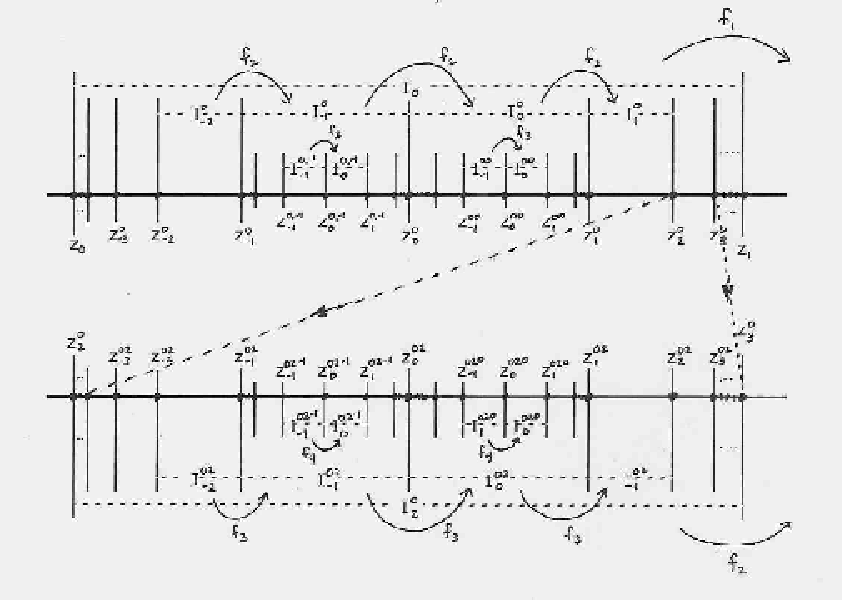
As we now wish to discuss the th step, at which point the indices begin to build up, we let be a word of letters, each letter an integer, specifying the location of the point with respect to the level orbit. By we mean the th letter in the word . When it is clear which word we are referring to (as in the case where we are dealing only with a particular point, or when we are using the word to specify all the points in a particular subinterval), we drop reference to the point and write merely or . We write to indicate the word of zeros.
Let our th generator be on . Extend to : if , ; and then extend to by shifting over and back by , etc., all the way down the chain of subintervals until is defined on all of (by shifting over and back by ). In this way preserves the orbits of the previous level orbit points, , and commutes with all the . Choose . We write .
As before, for the complete level n orbit we write
and generally
and for the intervals, we write . Note .
As acts like on , it gives an integer type picture in that interval, and the orbit in that interval accumulates at and . As all the generators commute, the orbit of is clearly an th order nested integer type, and has level .
An interesting question comes from a variation on the converse of this question; does the existence of a level orbit imply that the group must have at least a certain number of generators? We formulate a conjecture along these lines in Section 8.
5 Semigroups
We set aside groups for a moment and consider instead semigroups. The situation for semigroups is clearly different: because we are not guaranteed that semigroup elements will have inverses, we can not assume that all sets which are invariant under the action of the semigroup will intersect any particular middle subinterval we choose, as we did with groups in order to prove Lemma 2. Slightly different orbit structures can result from this, since we can not expect that nonempty minimal sets will exist inside each . We give an example to demonstrate one way in which this can effect the orbit structure of points.
5.1 The Idea
We wish to construct an example of a semigroup such that certain orbits do not fall into one of the four cases given for group orbits. The general idea is the following:
Consider two maps, and , taking to itself. Both maps will have a single fixed point inside the interval, one nearer to 0 and one nearer to 1. The fixed points will both be sources. Then any point to the outer side of either fixed point will only be able to move farther towards the edge. But points that sit between the two fixed points will be moved in opposite directions by and . If and are “incommensurate” in this area, they may create orbits that are dense between the fixed points.
In order to give an example of such a semigroup, we will actually use four maps: two that behave as described above, and two additional maps which will allow points to shift back towards the middle section. In the middle of the interval, we will design and to look like the example we gave for groups with a level 1 dense orbit.
5.2 The Maps
First we pick six points of : . The should be evenly spaced: . Let , and . The maps will be defined piecewise over these regions.
First, we give the two maps whose purpose is transportation. Note that the desired effect of sending points back towards the middle is achieved, as and by strict translation.
Next we give the two maps that represent the original concept. The important part is their action on : acts like and acts like . The functions could be filled in however we liked in the other sections, so long as fixed and fixed .
By combining these maps with the translations, we make the maps and , both of which take to itself. These two maps commute; the details of this are straighforward, but lengthy, and so they are omitted.
We let be the semigroup generated by , and , and we denote the orbit of under the semigroup by (the notation corresponds to that of the forward orbit of under a full group).
It should seem intuitive now that and are sufficiently incommensurate in the region that points in that region can be moved densely throughout that region.
Theorem 6.
For (repsectively ), has integer type in (resp. ), i.e. it is a countable collection of points that accumulates exactly at (resp. ), and . For , on the other hand, and are integer type, but is dense.
The proof follows easily from the fact that and are incommensurate.
6 A Closer Look at Case 4
We now return to full groups. In order to further understand the analysis of Case 4, we look at the intersection of the orbit and the subinterval that sits between two consecutive points of a lower level orbit. We examine the subgroup of consisting of homeomorphisms that preserve those subintervals . The intent is to restrict ourselves to an area where we can apply Lemma 2 again, and achieve the same conclusions as Theorem 3, with playing the role of , and the subgroup playing the role of . Throughout this section, we assume that the chosen lower level orbit has integer or Cantor set type, and we use to denote the intervals complementary to . We will use and interchangebly, depending on whether we mean to emphasize that it is the endpoint of the interval . We have a few lemmas.
6.1 Some Useful Lemmas
Let . This is clearly a subgroup of . Let .
Lemma 6.
If , then .
Proof: Let . So and for some , . Group elements must take complementary intervals to other complementary intervals, so this means , and .
Let . Then for some . Clearly .
Therefore, in order to get a picture of the group orbit of a point in a given subinterval, it is enough to look at the orbit of the point under the subgroup of homeomorphisms sending the interval to itself.
Lemma 7.
If has integer type, for all pairs of integers , there exists some such that .
Proof: Every group element must take intervals to other intervals, As the maps are all continuous, is totally determined by where takes an endpoint . As each endpoint is part of the orbit of , there is some with and some with . Therefore and so .
Lemma 8.
If has integer type, then for all and
Proof: Suppose takes to . Then by the fact that is continuous and the intervals are adjacent, it is clear that for all , must take to . Chose such that . Then as well. The argument is symmetric, so .
In this case ( of integer type) we shall refer to the subgroup of elements that take each to itself as , and we have:
Lemma 9.
If there exists a level 2 orbit, is nontrivial.
Proof: Suppose is a level 2 orbit point and . accumulates along , so there are infinitely many points of in . Pick some ; then for some group element . That group element is clearly in as it takes a point of to another point of , and it is nontrivial as .
In the case that has Cantor set type, it is not immediately clear that each subinterval is a homeomorphic copy of . Because the orbit of is merely dense in the Cantor set, but not necessarily equal to the Cantor set, we can not always find a map taking to another particular endpoint. However, the group orbit will look the same in those subintervals for which there is such a map.
6.2 Parallel Orbits and Subdivisions
Definition 3.
If are the intervals making up the complement of , and if for all consists of one point, we say that is parallel to .
Lemma 10.
If has integer type, then any parallel orbit is also integer type, and has the same level.
If has Cantor set type, what does a parallel orbit look like? The orbit consists of a single point in each open interval that is part of the complement of the Cantor set. We know the orbit accumulates along the endpoints of the Cantor set, since it is part of the range of the Cantor set orbit. In this case it does so in a one-sided manner, by which we mean that the accumulation set at any particular endpoint of an interval will consist of points which are not contained in , but sit exclusively to the other side of the endpoint. Therefore the orbit of is not integer type, but neither is it inside the Cantor set; the closure looks like the a Cantor set and the union of a countable collection of isolated points. Unlike an orbit parallel to an integer type orbit, this orbit will have a higher level, since it will, by necessity, accumulate at the Cantor set to which it is parallel.
Remark: The above description demonstrates that the concept parallel is not symmetric: may be parallel to without being parallel to .
For example, let be a homeomorphism with for in . Let be a point with integer type orbit, and the complementary intervals. Choose a point . We let for , and for , let be any homeomorphism. Now all will have an integer type orbit which intersects each in exactly one point. Thus we have a whole interval of orbits parallel to that of . Points of with will have more complicated orbits, depending on the interaction of and in that areas.
Lemma 11.
If is integer type, and if contains exactly one point, then for all , contains exactly one point, i.e., is parallel to .
Proof: Fix . From Lemma 7 we have some taking to . It is a homeomorphism, so contains exactly one point as well.
It is useful to note that if accumulates at , and has integer type, then any orbits parallel to must sit exclusively to one side or the other of . In other words, if and is parallel to , then the set is contained completely in or . This is because any element will fix the (single) point of and send each half of the interval to itself. Therefore, a single parallel orbit relegates the orbit of to one side or the other of , and if follows, of each . In order for to accumulate at , it must not be restricted to an interior subinterval. (If were of Cantor set type, the complementary intervals would not be adjacent, and a parallel orbit would not restrict other points from accumulating along . In fact, the orbits of all points complementary to the Cantor set will accumulate along the Cantor set: see the proof of Theorem 3) This means all parallel integer type orbits will sit to the same side of , and to the same side of all the points of . In this vein, when considering the behavior of in an interval , it is reasonable to restrict to a subinterval of in which there are no parallel orbits to : for instance, will be such an interval if is the rightmost parallel orbit point in . We call this subinterval , and its homeomorphic images in each we call . Note that elements of will also take each to itself.
Lemma 12.
, and therefore the group orbit of intersected with can not be topologically different from the that of intersected with any other .
Proof: Let . The equality is given by Lemma 7. As the orbit of intersected with any given contains the homeomorphic image of the orbit of intersected with , and vice versa, the two pictures are topologically equivalent.
We know that it is impossible for to have a Cantor set orbit in one and an integer type orbit in another, or to be dense in one and contained in a Cantor set in another. However, the orbit of may be different in seperate subintervals of , bounded by points of various parallel orbits, as elements of may behave in different ways on different subintervals of a given .
For both the integer type and the Cantor set type, we can restrict ourselves to looking at a single , bounded by consecutive points of some lower level orbit, and develop the picture there. (In the integer case, we need only look at one subinterval, because the orbit will be the same in all subintervals.) If the lower level orbit has orbits which are parallel to it, we may want to break the down into subintervals bounded by points of parallel orbits. We expect that in each subinterval, we have a repetition of the main picture: dense orbits, a Cantor set, integer type, and possibly higher levels. However, in order to conclude that our restriction again falls into one of the original four cases, we need to be able to apply Lemma 2 to the subgroup of associated to that interval. Unfortunately, we do not know if either of the conditions are satisfied: subgroups of finitely generated groups are not necessarily themselves finitely generated, and we do not have enough information about the maps in the subgroups to conclude that one of them is free of accumulating fixed points. In order to conclude anything additional, we therefore require additional hypotheses.
7 Analytic Groups
Theorem 7.
If is a finitely generated group of homeomorphisms of the interval which are continuous on and analytic on , and if there are no fixed points of the group in , then there can be at most one integer type orbit with level greater than 1. In addition, if is a level integer type orbit, and it intersects some (an interval complementary to the level orbit), all other orbits intersecting will be parallel to , i.e., they will all be level integer type orbits. Therefore there will be no orbits of level greater than in and its homeomorphic copies.
Proof:
Since is finitely generated and there are no fixed points of the group inside , we can apply Lemma 2 to find a -minimal set inside . As in Theorem 3, we can apply minimality arguments to conclude that must fall into one of the four cases. Let us assume it is a level integer type orbit, where is greater than 1. Let be the level orbit on which accumulates. Since has integer type, must have integer or Cantor set type. In either case, let be the collection of complementary intervals, such that . Since has level integer type, we can further divide into subintervals complementary to the orbit of , which we call .
Consider the subgroup . is clearly nontrivial as intersects in an infinite number of points. But what about ? We note that for all , since the are adjacent. But this means that has a sequence of fixed points accumulating at the endpoints of , namely, the endpoints of the . Since is interior to , and is analytic in , this means must be the identity map. Therefore every point has an orbit which intersects each in exactly one point, giving it an orbit parallel to that of , level integer type. Thus is the highest order level for orbits of points in .
Theorem 8.
If is a finitely generated abelian group of homeomorphisms of which are continuous on and analytic on , there can be no orbits of Cantor set type. Therefore the highest possible non-dense orbit is level 2 integer type.
Proof:
Suppose were Cantor set type. Let be the collection of intervals complementary to the Cantor set, and say is the left endpoint of the interval . Consider . The orbit of is dense in the Cantor set, so if is the left endpoint of , there must be a sequence of maps such that , and is mapped to the corresponding intervals . Consider . Since , then if , . Because is abelian, this means . So has each as a fixed point, and the accumulate at . However, is analytic in , and is interior to . This is a contradiction. So must not be Cantor set type. Therefore, if is not dense, it must be either level 1 integer type, or level 2 integer type (accumulating along a level 1 integer type). It can not be level 3, by Theorem 7.
8 Questions and Conjectures
We would like to be able to make a definitive statement about the overall structure of orbits of points in Case 4. It seems that the natural thing to expect is that orbits in Cases 1, 2, or 3 “nest” at increasing levels, such that the orbit of a level point can be understood by first looking at a single interval, broken down into subintervals bounded by consecutive parallel orbits, such that in each section the orbit will be dense, integer type, or contained in a Cantor set. That picture will then be repeated a countable number of times at each level. However, in order to conclude this, we must better understand the structure of the subgroups that preserve subintervals at a given level. It seems likely that some amount of additional smoothness of the generators will enable us to apply the crucial lemma to the subgroups. We expect that we need something stronger than continuity, but that it is not necessary to require as much as analyticity:
Conjecture 1.
If is a group generated by homeomorphisms, orbits of points in Case 4 will consist of a countable number of copies of an interval , the union of a number of subintervals , in each of which the orbit is dense, has integer type, or is contained in a Cantor set.
Without knowing exactly how much smoothness is required, it would be interesting to see an example of a group of homeomorphisms with a level 1 integer type orbit where the subgroup that preserves the subintervals does not satisfy either condition in Lemma 2. One imagines that the generating homeomorphisms of such a group would be quite complicated, either individually or in their interaction.
It seems likely that more statements could be made about the level orbits that are possible under a particular group:
Conjecture 2.
If is a group generated by homeomorphisms, the highest possible level of an orbit is .
There are also natural questions about the effect of the group structure on the possible orbits. We saw that the addition of abelian to the analytic case greatly restricted the possibilities. In particular, if the group is abelian, it may simplify the complications created by an orbit accumulating along a Cantor set. What effect might abelian have on a group of less smooth homeomorphisms? What about other group structure restrictions? This issue is partially addressed in [1].
Finally, in the case of semigroups, although the structures can clearly be different, there is probably a similar description for orbits which takes into account any sections of the circle where all maps move points in the same direction.
References
- [1] Benson Farb and John Franks, Groups of Homeomorphisms of One-Manifolds III: Nilpotent Subgroups. Ergodic Theory and Dynam. Syst., 2001
- [2] Etienne Ghys, Groups Acting on the Circle, IMCA, Lima, 1999
- [3] Anatole Katok and Boris Hasselblatt, Introduciton to the Modern Theory of Dynamical Systems, Cambridge University Press, New York, 1995
- [4] Charles Pugh, Introduction to Analysis, Springer, New York, 2000
- [5] Clark Robinson, Dynamical Systems: Stability, Symbolic Dynamics, and Chaos, CRC Press, Boca Raton, 1998