On the Metric Dimension of
Cartesian Products of GraphsThanks: Research supported by projects MCYT-FEDER-BFM2003-00368, Gen-Cat-2001SGR00224, MCYT-HU2002-0010, MTM-2004-07891-C02-01, MEC-SB2003-0270, MCYT-FEDER BFM2003-00368, and Gen. Cat 2001SGR00224.

José Cáceres Address: Departamento de Estadística y Matemática Aplicada, Universidad de Almería, Almería, Spain Email address: jcaceres@ual.es , Carmen Hernando Address: Departament de Matemàtica Aplicada I, Universitat Politècnica de Catalunya, Barcelona, Spain Email address: carmen.hernando@upc.edu , Mercè Mora Address: Departament de Matemàtica Aplicada II, Universitat Politècnica de Catalunya, Barcelona, Spain Email address: merce.mora@upc.edu , Ignacio M. Pelayo Address: Departament de Matemàtica Aplicada III, Universitat Politècnica de Catalunya, Barcelona, Spain Email address: ignacio.m.pelayo@upc.edu , María L. Puertas Address: Departamento de Estadística y Matemática Aplicada, Universidad de Almería, Almería, Spain Email address: mpuertas@ual.es , Carlos Seara Address: Departament de Matemàtica Aplicada II, Universitat Politècnica de Catalunya, Barcelona, Spain Email address: carlos.seara@upc.edu and David R. Wood Address: Departament de Matemàtica Aplicada II, Universitat Politècnica de Catalunya, Barcelona, Spain Email address: david.wood@upc.edu

Abstract.

A set of vertices $S$ resolves a graph $G$ if every vertex is uniquely determined by its vector of distances to the vertices in $S$ . The metric dimension of $G$ is the minimum cardinality of a resolving set of $G$ . This paper studies the metric dimension of cartesian products $G\,\square\,H$ . We prove that the metric dimension of $G\,\square\,G$ is tied in a strong sense to the minimum order of a so-called doubly resolving set in $G$ . Using bounds on the order of doubly resolving sets, we establish bounds on $G\,\square\,H$ for many examples of $G$ and $H$ . One of our main results is a family of graphs $G$ with bounded metric dimension for which the metric dimension of $G\,\square\,G$ is unbounded.

Key words and phrases:

graph, distance, resolving set, metric dimension, metric basis, cartesian product, Hamming graph, Mastermind, coin weighing

2000 Mathematics Subject Classification

05C12 (distance in graphs)

1. Introduction

A set of vertices $S$ resolves a graph $G$ if every vertex of $G$ is uniquely determined by its vector of distances to the vertices in $S$ . This paper undertakes a general study of resolving sets in cartesian products of graphs.

All the graphs considered are finite, undirected, simple, and connected¹¹ 1 The results can easily be generalised to disconnected graphs; we omit the details.. The vertex set and edge set of a graph $G$ are denoted by $V(G)$ and $E(G)$ . The distance between vertices $v,w\in V(G)$ is denoted by $d_{G}(v,w)$ , or $d(v,w)$ if the graph $G$ is clear from the context. A vertex $x\in V(G)$ resolves a pair of vertices $v,w\in V(G)$ if $d(v,x)\neq d(w,x)$ . A set of vertices $S\subseteq V(G)$ resolves $G$ , and $S$ is a resolving set of $G$ , if every pair of distinct vertices of $G$ are resolved by some vertex in $S$ . A resolving set $S$ of $G$ with the minimum cardinality is a metric basis of $G$ , and $|S|$ is the metric dimension of $G$ , denoted by $\beta(G)$ .

The cartesian product of graphs $G$ and $H$ , denoted by $G\,\square\,H$ , is the graph with vertex set $V(G)\times V(H):=\{(a,v):a\in V(G),v\in V(H)\}$ , where $(a,v)$ is adjacent to $(b,w)$ whenever $a=b$ and $\{v,w\}\in E(H)$ , or $v=w$ and $\{a,b\}\in E(G)$ . Where there is no confusion the vertex $(a,v)$ of $G\,\square\,H$ will be written $av$ . Observe that if $G$ and $H$ are connected, then $G\,\square\,H$ is connected. In particular, for all vertices $av,bw$ of $G\,\square\,H$ we have $d(av,bw)=d_{G}(a,b)+d_{H}(v,w)$ . Assuming isomorphic graphs are equal, the cartesian product is associative, and $G_{1}{\,\square\,}G_{2}{\,\square\,}\cdots{\,\square\,}G_{d}$ is well-defined.

Resolving sets in general graphs were first defined by Harary and Melter 1976 and Slater 1975, although as we shall see, resolving sets in hypercubes were studied earlier under the guise of a coin weighing problem [23, 13, 6, 25, 1, 27, 37, 14, 5, 20, 24, 18, 26]. Resolving sets have since been widely investigated [34, 31, 30, 10, 33, 4, 28, 12, 39, 8, 9, 38, 21, 40, 32, 7, 36, 29], and arise in many diverse areas including network discovery and verification [2], robot navigation [21, 34], connected joins in graphs [33], and strategies for the Mastermind game [3, 17, 15, 16, 20, 11].

Part of our motivation for studying the metric dimension of cartesian products is that in two of the above-mentioned applications, namely Mastermind and coin weighing, the graphs that arise are in fact cartesian products. These connections are explained in Sections 2 and 6 respectively.

The main contributions of this paper are based on the notion of doubly resolving sets, which are introduced in Section 4. We prove that the minimum order of a doubly resolving set in a graph $G$ is tied in a strong sense to $\beta(G\,\square\,G)$ . Thus doubly resolving sets are essential in the study of metric dimension of cartesian products. We then give a number of examples of bounds on the metric dimension of cartesian products through doubly resolving sets. In particular, Sections 5, 6, 7, 8, and 9 respectively study complete graphs, Hamming graphs, paths and grids, cycles, and trees. One of our main results here is a family of (highly connected) graphs with bounded metric dimension for which the metric dimension of the cartesian product is unbounded.

2. Coin Weighing and Hypercubes

The hypercube $Q_{n}$ is the graph whose vertices are the $n$ -dimensional binary vectors, where two vertices are adjacent if they differ in exactly one coordinate. It is well known that

Q_{n}=\underbrace{K_{2}{\,\square\,}K_{2}{\,\square\,}\cdots{\,\square\,}K_{2}}_{n}.

It is easily seen that $\beta(Q_{n})\leq n$ (see Equation (11)). The first case when this bound is not tight is $n=5$ . A laborious calculation verifies that $Q_{5}$ is resolved by the $4$ -vertex set $\{00000,00011,00101,01001\}$ . We have determined $\beta(Q_{n})$ for small values of $n$ by computer search.

$n$	$2$	$3$	$4$	$5$	$6$	$7$	$8$	$10$	$15$
$\beta(Q_{n})$	$2$	$3$	$4$	$4$	$5$	$6$	$6$	$\leq 7$	$\leq 10$

The asymptotic value of $\beta(Q_{n})$ turns out to be related to the following coin weighing problem first posed by Söderberg and Shapiro 1963. (See [18] for a survey on various coin weighing problems.) Given $n$ coins, each with one of two distinct weights, determine the weight of each coin with the minimum number of weighings. We are interested in the static variant of this problem, where the choice of sets of coins to be weighed is determined in advance. Weighing a set $S$ of coins determines how many light (and heavy) coins are in $S$ , and no further information. It follows that the minimum number of weighings differs from $\beta(Q_{n})$ by at most one [33, 20]. A lower bound on the number of weighings by Erdős and Rényi 1963 and an upper bound by Lindström 1964 imply that

\lim_{n\rightarrow\infty}\,\beta(Q_{n})\cdot\frac{\log n}{n}=2,

where, as always in this paper, logarithms are binary. Note that Lindstrom’s proof is constructive. He gives an explicit scheme of $2^{k}-1$ weighings that suffice for $k\cdot 2^{k-1}$ coins.

3. Projections

Let $S$ be a set of vertices in the cartesian product $G\,\square\,H$ of graphs $G$ and $H$ . The projection of $S$ onto $G$ is the set of vertices $a\in V(G)$ for which there exists a vertex $av\in S$ . Similarly, the projection of $S$ onto $H$ is the set of vertices $v\in V(H)$ for which there exists a vertex $av\in S$ . A column of $G\,\square\,H$ is the set of vertices $\{av:v\in V(H)\}$ for some vertex $a\in V(G)$ , and a row of $G\,\square\,H$ is the set of vertices $\{av:a\in V(G)\}$ for some vertex $v\in V(H)$ . Observe that each row induces a copy of $G$ , and each column induces a copy of $H$ . This terminology is consistent with a representation of $G\,\square\,H$ by the points of the $|V(G)|\times|V(H)|$ grid.

Lemma 3.1.

Let $S\subseteq V(G\,\square\,H)$ for graphs $G$ and $H$ . Then every pair of vertices in a fixed row of $G\,\square\,H$ are resolved by $S$ if and only if the projection of $S$ onto $G$ resolves $G$ . Similarly, every pair of vertices in a fixed column of $G\,\square\,H$ are resolved by $S$ if and only if the projection of $S$ onto $H$ resolves $H$ .

Proof.

Consider two vertices $av$ and $aw$ in a common column. For every other vertex $bx$ of $G\,\square\,H$ , we have $d(av,bx)-d(aw,bx)=d_{H}(v,x)-d_{H}(w,x)$ . Thus $d(av,bx)\neq d(aw,bx)$ if and only if $d_{H}(v,x)\neq d_{H}(w,x)$ . That is, $av$ and $aw$ are resolved by $bx$ if and only if $v$ and $w$ are resolved by $x$ in $H$ . Hence $av$ and $aw$ are resolved by $S$ if and only if $v$ and $w$ are resolved by the projection of $S$ onto $H$ . We have the analogous result for the projection onto $G$ by symmetry.∎

Corollary 3.2.

For all graphs $G$ and $H$ , and for every resolving set $S$ of $G\,\square\,H$ , the projection of $S$ onto $G$ resolves $G$ , and the projection of $S$ onto $H$ resolves $H$ . In particular, $\beta(G\,\square\,H)\geq\max\{\beta(G),\beta(H)\}$ .∎

4. Doubly Resolving Sets

Many of the results that follow are based on the following definitions. Let $G\neq K_{1}$ be a graph. Two vertices $v,w\in V(G)$ are doubly resolved by $x,y\in V(G)$ if

d(v,x)-d(w,x)\neq d(v,y)-d(w,y).

A set of vertices $S\subseteq V(G)$ doubly resolves $G$ , and $S$ is a doubly resolving set, if every pair of distinct vertices $v,w\in V(G)$ are doubly resolved by two vertices in $S$ . Every graph with at least two vertices has a doubly resolving set. Let $\psi(G)$ denote the minimum cardinality of a doubly resolving set of a graph $G\neq K_{1}$ . Note that if $x,y$ doubly resolves $v,w$ then $d(v,x)-d(w,x)\neq 0$ or $d(v,y)-d(w,y)\neq 0$ , and at least one of $x$ and $y$ (singly) resolves $v,w$ . Thus a doubly resolving set is also a resolving set, and

\beta(G)\leq\psi(G).

Our interest in doubly resolving sets is based on the following upper bound.

Theorem 4.1.

For all graphs $G$ and $H\neq K_{1}$ ,

\beta(G\,\square\,H)\leq\beta(G)+\psi(H)-1.

Proof.

Let $S$ be a metric basis of $G$ . Let $T$ be a doubly resolving set of $H$ with $|T|=\psi(H)$ . Fix vertices $s\in S$ and $t\in T$ . Let

X:=\{sv:v\in T\}\cup\{at:a\in S\}.

Observe that $|X|=|S|+|T|-1$ . To prove that $X$ resolves $G\,\square\,H$ , consider two vertices $av$ and $bw$ of $G\,\square\,H$ . By Lemma 3.1, if $a=b$ then $av$ and $bw$ are resolved since the projection of $X$ onto $H$ is $T$ . Similarly, if $v=w$ then $av$ and $bw$ are resolved since the projection of $X$ onto $G$ is $S$ . Now assume that $a\neq b$ and $v\neq w$ . Since $T$ is doubly resolving for $H$ , there are two vertices $x,y\in T$ such that

d_{H}(v,x)-d_{H}(w,x)\neq d_{H}(v,y)-d_{H}(w,y).

Thus for at least one of $x$ and $y$ , say $x$ , we have

d_{H}(v,x)-d_{H}(w,x)\neq d_{G}(b,s)-d_{G}(a,s).

Hence

d(av,sx)=d_{G}(a,s)+d_{H}(v,x)\neq d_{G}(b,s)+d_{H}(w,x)=d(bw,sx).

That is, $sx\in X$ resolves $av$ and $bw$ .∎

The relationship between resolving sets of cartesian products and doubly resolving sets is strengthened by the following lower bound.

Lemma 4.2.

Suppose that $S$ resolves $G\,\square\,G$ for some graph $G$ . Let $A$ and $B$ be the two projections of $S$ onto $G$ . Then $A\cup B$ doubly resolves $G$ . In particular,

\beta(G\,\square\,G)\geq\tfrac{1}{2}\psi(G).

Proof.

For any two vertices $v,w\in V(G)$ , there is a vertex $pq\in S$ that resolves $vw,wv$ . That is, $d(vw,pq)\neq d(wv,pq)$ . Thus $d(v,p)+d(w,q)\neq d(w,p)+d(v,q)$ , which implies $d(v,p)-d(w,p)\neq d(v,q)-d(w,q)$ . Thus $p,q$ doubly resolves $v,w$ in $G$ . Now $p\in A$ and $q\in B$ . Hence $A\cup B$ doubly resolves $G$ . If, in addition, $S$ is a metric basis of $G\,\square\,G$ , then $\psi(G)\leq|A\cup B|\leq|A|+|B|\leq 2|S|=2\cdot\beta(G\,\square\,G)$ .∎

Observe that Theorem 4.1 and Lemma 4.2 prove that $\beta(G\,\square\,G)$ is always within a constant factor of $\psi(G)$ . In particular,

(1)

\tfrac{1}{2}\psi(G)\leq\beta(G\,\square\,G)\leq\psi(G)+\beta(G)-1\leq 2\psi(G)-1.

Thus doubly resolving sets are essential in the study of the metric dimension of cartesian products.

A natural candidate for a resolving set of $G\,\square\,G$ is $S\times S$ for a well chosen set $S\subseteq V(G)$ . It follows from Lemma 4.2 and the proof technique employed in Theorem 4.1 that $S\times S$ resolves $G\,\square\,G$ if and only if $S$ doubly resolves $G$ .

Now consider the following elementary bound on $\psi(G)$ .

Lemma 4.3.

For every graph $G$ with $n\geq 3$ vertices we have $\psi(G)\leq n-1$ .

Proof.

Clearly $G$ has a vertex $x$ of degree at least two. Let $S:=V(G)\setminus\{x\}$ . To prove that $S$ doubly resolves $G$ , consider two vertices $u,v\in V(G)$ . If both $u,v\in S$ , then the pair $u,v$ doubly resolves itself. Otherwise, without loss of generality, $u\in S$ and $v=x$ . Since $\deg(x)\geq 2$ , there is a neighbour $y\neq u$ of $x$ . Now $d(u,u)-d(v,u)\leq 0-1=-1$ and $d(u,y)-d(v,y)\geq 1-1=0$ . Thus $u,y\in S$ doubly resolve $u,v$ . Hence $S$ doubly resolves $G$ .∎

Note that if $G$ is a graph with $n\geq 3$ vertices, then Theorem 4.1 and Lemma 4.3 imply that $\beta(G\,\square\,H)\leq\beta(H)+n-2$ for every graph $H$ .

5. Complete Graphs

Let $K_{n}$ denote the complete graph on $n\geq 1$ vertices. It is well known [21, 8] that for every $n$ -vertex graph $G$ ,

(2)

\beta(G)=n-1\,\Longleftrightarrow\,G=K_{n}.

Lemma 5.1.

For all $n\geq 2$ we have $\psi(K_{n})=\max\{n-1,2\}$ .

Proof.

Since $\psi(G)\geq 2$ for every graph $G\neq K_{1}$ , we have $\psi(K_{2})=2$ . Now suppose that $n\geq 3$ . By Lemma 4.3, $\psi(K_{n})\leq n-1$ . Conversely, $\psi(K_{n})\geq\beta(K_{n})=n-1$ by Equation (2).∎

Theorem 4.1 and Lemma 5.1 imply that every graph $G$ satisfies

(3)

\beta(K_{n}\,\square\,G)\leq\beta(G)+\max\{n-2,1\}.

In certain cases, this result can be improved as follows.

Lemma 5.2.

For every graph $G$ and for all $n\geq 1$ ,

\beta(K_{n}\,\square\,G)\leq\max\{n-1,2\cdot\beta(G)\}.

Proof.

Let $S$ be a metric basis of $G$ . Fix a vertex $r$ of $K_{n}$ . As illustrated in Figure 1, there is a set $T$ of $\max\{n-1,2|S|\}$ vertices of $K_{n}\,\square\,G$ such that:

(a)

for all vertices $a\in V(K_{n})\setminus\{r\}$ , there is at least one vertex $x\in S$ for which $ax\in T$ , and
(b)

for all $x\in S$ , there are at least two vertices $a,b\in V(K_{n})$ for which $ax\in T$ and $bx\in T$ .

Refer to caption — Figure 1. The resolving set $T$ of $K_{n}\,\square\,G$ in Lemma 5.2: (a) $n-1\geq 2\beta(G)$ and (b) $n-1\leq 2\beta(G)$ .

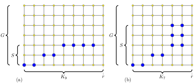
To prove that $T$ resolves $K_{n}\,\square\,G$ , consider two vertices $av$ and $bw$ of $K_{n}\,\square\,G$ . If $v=w$ , then since the projection of $T$ onto $G$ is the resolving set $S$ , by Lemma 3.1, $av$ and $bw$ are resolved by $T$ . Now suppose that $v\neq w$ . Then there is a vertex $x\in S$ that resolves $v$ and $w$ in $G$ . Hence $d_{G}(v,x)<d_{G}(w,x)$ without loss of generality. By (b) there are distinct vertices $c,d\in V(K_{n})$ for which $cx\in T$ and $dx\in T$ . If $c\neq a$ and $c\neq b$ , then

d(av,cx)=d_{G}(v,x)+1<d_{G}(w,x)+1=d(bw,cx));

that is, $cx$ resolves $av$ and $bw$ in $K_{n}\,\square\,G$ . Similarly, if $d\neq a$ and $d\neq b$ , then $dx$ resolves $av$ and $bw$ . Otherwise $c=a$ or $c=b$ , and $d=a$ or $d=b$ . Since $c\neq d$ , without loss of generality $c=a$ and $d=b$ . Then

d(av,cx)=d_{G}(v,x)<d_{G}(w,x)<d_{G}(w,x)+1=d(bw,cx),

and again $cx$ resolves $av$ and $bw$ in $K_{n}\,\square\,G$ .∎

When is $n$ is large in comparison with $\beta(G)$ we know $\beta(K_{n}\,\square\,G)$ exactly.

Theorem 5.3.

For every graph $G$ and for all $n\geq 2\cdot\beta(G)+1$ ,

\beta(K_{n}\,\square\,G)=n-1.

Proof.

The lower bound $\beta(K_{n}\,\square\,G)\geq n-1$ follows from Corollary 3.2 and Equation (2). The upper bound $\beta(K_{n}\,\square\,G)\leq n-1$ is a special case of Lemma 5.2.∎

6. Mastermind and Hamming Graphs

Mastermind is a game for two players, the code setter and the code breaker²² 2 Chvátal 1983 referred to the code setter and code breaker as S.F. and P.G.O.M. (in honour of P.E.).. The code setter chooses a secret vector $s=[s_{1},s_{2},\dots,s_{n}]\in\{1,2,\dots,k\}^{n}$ . The task of the code breaker is to infer the secret vector by a series of questions, each a vector $t=[t_{1},t_{2},\dots,t_{n}]\in\{1,2,\dots,k\}^{n}$ . The code setter answers with two integers, first being the number of positions in which the secret vector and the question agree, denoted by $a(s,t)=|\{i:s_{i}=t_{i},1\leq i\leq n\}|$ . The second integer $b(s,t)$ is the maximum of $a(\tilde{s},t)$ , where $\tilde{s}$ ranges over all permutations of $s$ .

In the commercial version of the game, $n=4$ and $k=6$ . The secret vector and each question is represented by four pegs each coloured with one of six colours. Each answer is represented by $a(s,t)$ black pegs, and $b(s,t)-a(s,t)$ white pegs. Knuth 7677 showed that four questions suffice to determine $s$ in this case. Here the code breaker may determine each question in response to the previous answers. Static mastermind is the variation in which all the questions must be supplied at once. Let $g(n,k)$ denote the maximum, taken over all vectors $s$ , of the minimum number of questions required to determine $s$ in this static setting.

The Hamming graph $H_{n,k}$ is the cartesian product of cliques

H_{n,k}=\underbrace{K_{k}{\,\square\,}K_{k}{\,\square\,}\cdots{\,\square\,}K_{k}}_{n}.

Note that the hypercube $Q_{n}=H_{n,2}$ . The vertices of $H_{n,k}$ can be thought of as vectors in $\{1,2,\dots,k\}^{n}$ , with two vertices being adjacent if they differ in precisely one coordinate. Thus the distance $d_{H}(v,w)$ between two vertices $v$ and $w$ is the number of coordinates in which their vectors differ. That is,

d_{H}(v,w)=n-a(v,w).

Suppose for the time being that we remove the second integer $b(s,t)$ from the answers given by the code setter in the static mastermind game. Let $f(n,k)$ denote the maximum, taken over all vectors $s$ , of the minimum number of questions required to determine $s$ without $b(s,t)$ in the answers. For the code breaker to correctly infer the secret vector $s$ from a set of questions $T$ , $s$ must be uniquely determined by the values $\{a(s,t):t\in T\}$ . Equivalently, for any two vertices $v$ and $w$ of $H_{n,k}$ , there is a $t\in T$ for which $a(v,t)\neq a(w,t)$ ; that is, the distances $d_{H}(v,t)\neq d_{H}(w,t)$ . Hence the secret vector can be inferred if and only if $T$ resolves $H_{n,k}$ . Thus

g(n,k)\leq f(n,k)=\beta(H_{n,k}).

Chvátal 1983 proved the upper bound

\beta(H_{n,k})=f(n,k)\leq(2+\epsilon)n\,\frac{1+2\log k}{\log n-\log k}

for large $n>n(\epsilon)$ and small $k<n^{1-\epsilon}$ . For $k\in\{3,4\}$ , improvements to the constant in the above upper bound are stated without proof by Kabatianski et al. 2000. They also state that a ‘straightforward generalisation’ of the lower bound on $\beta(Q_{n})$ by Erdős and Rényi 1963 gives for large $n$ ,

\beta(H_{n,k})\geq g(n,k)\geq(2+o(1))\frac{n\log k}{\log n}.

Here we study $\beta(H_{n,k})$ for large values of $k$ rather that for large values of $n$ . A similar approach is take by Goddard 2003, Goddard 2004 for static Mastermind, who proved that $g(2,k)=\lceil\frac{2}{3}k\rceil$ and $g(3,k)=k-1$ . Our contribution is to determine the exact value of $\beta(H_{2,k})$ . We show that for all $k\geq 1$ ,

(4)

\beta(H_{2,k})=\left\lfloor\tfrac{2}{3}(2k-1)\right\rfloor.

Equation (4) is a special case (with $m=n=k$ ) of the following more general result.

Theorem 6.1.

For all $n\geq m\geq 1$ we have

\beta(K_{n}\,\square\,K_{m})=\begin{cases}\left\lfloor\tfrac{2}{3}(n+m-1)\right\rfloor&\textup{, if }m\leq n\leq 2m-1\\ n-1&\textup{, if }n\geq 2m-1.\end{cases}

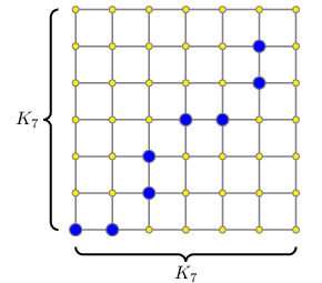
Note that two vertices of $K_{n}\,\square\,K_{m}$ are adjacent if and only if they are in a common row or column. Otherwise they are at distance two. Fix a set $S$ of vertices of $K_{n}\,\square\,K_{m}$ . With respect to $S$ , a row or column is empty if it contains no vertex in $S$ , and a vertex $v\in S$ is lonely if $v$ is the only vertex of $S$ in its row and in its column. As illustrated in Figure 2, we have the following characterisation of resolving sets in $K_{n}\,\square\,K_{m}$ .

Lemma 6.2.

For $m,n\geq 2$ , a set $S$ of vertices resolves $K_{n}\,\square\,K_{m}$ if and only if:

(a)

there is at most one empty row and at most one empty column,
(b)

there is at most one lonely vertex, and
(c)

if there is an empty row and an empty column, then there is no lonely vertex.

Proof.

( $\Longrightarrow$ ) First suppose that $S$ resolves $K_{n}\,\square\,K_{m}$ . By Corollary 3.2, the projections of $S$ respectively resolve $K_{m}$ and $K_{n}$ . By Equation (2), there is at most one empty row and at most one empty column. Thus (a) holds.

Suppose on the contrary that $v$ and $w$ are two lonely vertices in $S$ . Thus $v$ and $w$ are in distinct rows and columns, and no other vertex of $S$ is in a row or column that contains $v$ or $w$ . Let $x$ be the vertex in the row of $v$ and the column of $w$ . Let $y$ be the vertex in the column of $v$ and the row of $w$ . Then $d(x,v)=d(y,v)=1$ , $d(x,w)=d(y,w)=1$ , and $d(x,u)=d(y,u)=2$ for every vertex $u\in S\setminus\{v,w\}$ . Thus $S$ does not resolve $x$ and $y$ . This contradiction proves that $S$ satisfies (b).

Finally, suppose that there is an empty row, an empty column, and a lonely vertex $v\in S$ . Let $x$ be the vertex in the row of $v$ and in the empty column. Let $y$ be the vertex in the column of $v$ and in the empty row. We have $d(x,v)=d(y,v)=1$ , and $d(x,u)=d(y,u)=2$ for every vertex $u\in S\setminus\{v\}$ . Thus $S$ does not resolve $x$ and $y$ . This contradiction proves that $S$ satisfies (c).

( $\Longleftarrow$ ) Now suppose that $S$ is a set of vertices satisfying (a), (b) and (c). We will prove that $S$ resolves any two vertices $x$ and $y$ . If $x\in S$ , then $x$ resolves $x,y$ . If $y\in S$ , then $y$ resolves $x,y$ . Now suppose that $x\not\in S$ and $y\not\in S$ .

If $x$ and $y$ are in the same row, then at least one of the columns of $x$ and $y$ contains a vertex $v\in S$ . Suppose $v$ is in the column of $x$ . Thus $d(x,v)=1$ and $d(y,v)=2$ , and $v$ resolves $x,y$ . Similarly, if $x$ and $y$ are in the same column, then some $v\in S$ resolves $x,y$ .

Suppose now that $x$ and $y$ are in distinct rows and columns. Then there is a vertex of $S$ in the column of $x$ or in the column of $y$ . Suppose $v\in S$ is in the column of $x$ . If $v$ is not in the row of $y$ , $d(x,v)=1\neq 2=d(y,v)$ , and $v$ resolves $x,y$ . If $v$ is in the row of $y$ , by (b) and (c), at least one of the vertices in the rows and columns of $x$ and $y$ , but not in the intersection of two of them, is in $S$ . This vertex resolves $x$ and $y$ .∎

Lemma 6.3.

For all $n,m\geq 3$ , if $S$ resolves $K_{n}\,\square\,K_{m}$ , then there exists a resolving set $S^{*}$ of $K_{n}\,\square\,K_{m}$ such that $|S^{*}|\leq|S|$ , and $S$ contains two vertices $v$ and $w$ in the same row or column, such that $v$ and $w$ are the only vertices in $S^{*}$ in the row(s) and column(s) that contain $v$ and $w$ .

Proof.

By Lemma 6.2, there are two vertices $v,w\in S$ in the same row or column. By symmetry, we can suppose that $v$ and $w$ are in the same row. If $v$ and $w$ are the only vertices in $S^{*}$ in the row and columns that contain $v$ and $w$ , then we are done. Otherwise there is a vertex $x\in S$ in the row or columns that contain $v$ and $w$ . It suffices to prove that $x$ can be deleted from $S$ , or replaced in $S$ by some other vertex not in the row or columns that contain $v$ and $w$ , such that $S$ still satisfies the conditions of Lemma 6.2, and thus resolves $K_{n}\,\square\,K_{m}$ . We can then repeat this step to obtain the desired set $S^{*}$ .

First suppose that $x$ is in the same row as $v$ and $w$ . If all the vertices of the column of $x$ are in $S$ , then delete $x$ from $S$ ; clearly $S$ still satisfies the conditions of Lemma 6.2. Otherwise, let $y$ be a vertex not in $S$ such that $y$ is in the column containing $x$ , and if $x$ is the only vertex in its column that is in $S$ , then $y$ is in a row that contains at least one vertex of $S$ . This is always possible, since $S$ satisfies condition (a). Then $(S\setminus\{x\})\cup\{y\}$ satisfies the conditions of Lemma 6.2.

Now suppose that $x$ is in the column of $v$ or $w$ . If every vertex in the row containing $x$ is in $S$ , then delete $x$ from $S$ ; clearly $S$ still satisfies the the conditions of Lemma 6.2. Otherwise, proceeding as in the preceding case, let $y$ be a vertex in the same row as $x$ , but not in the columns of $v$ and $w$ , such that there is at least one other vertex of $S$ in the row or column that contains $y$ . Then $(S\setminus\{x\})\cup\{y\}$ satisfies the conditions of Lemma 6.2. This completes the proof.∎

Lemma 6.4.

For all $n,m\geq 3$ ,

\beta(K_{n}\,\square\,K_{m})=2+\min\{\beta(K_{n-2}\,\square\,K_{m-1}),\beta(K_{n-1}\,\square\,K_{m-2})\}.

Proof.

We first prove that

(5)

\beta(K_{n}\,\square\,K_{m})\leq 2+\min\{\beta(K_{n-2}\,\square\,K_{m-1}),\beta(K_{n-1}\,\square\,K_{m-2})\}.

Without loss of generality $\beta(K_{n-2}\,\square\,K_{m-1})\leq\beta(K_{n-1}\,\square\,K_{m-2})$ . Let $S$ be a metric basis of $K_{n-2}\,\square\,K_{m-1}$ . Construct $S^{\prime}\subseteq V(K_{n}\,\square\,K_{m})$ from $S$ by adding two new vertices that are positioned in one new row and in two new columns. The number of empty rows, empty columns, and lonely vertices is the same in $S$ and $S^{\prime}$ . Since $S$ resolves $K_{n-2}\,\square\,K_{m-1}$ , $S^{\prime}$ resolves $K_{n}\,\square\,K_{m}$ by Lemma 6.2. Thus $\beta(K_{n}\,\square\,K_{m})\leq|S^{\prime}|=|S|+2=2+\beta(K_{n-2}\,\square\,K_{m-1})$ , which implies (5). It remains to prove that

(6)

\min\{\beta(K_{n-2}\,\square\,K_{m-1}),\beta(K_{n-1}\,\square\,K_{m-2})\}\leq\beta(K_{n}\,\square\,K_{m})-2.

Let $S$ be a metric basis of $K_{n}\,\square\,K_{m}$ . By Lemma 6.3, we can assume that $S$ contains two vertices $v$ and $w$ in the same row or column, such that $v$ and $w$ are the only vertices in $S$ in the row(s) and column(s) that contain $v$ and $w$ . Without loss of generality, $v$ and $w$ are in the same row. Construct $S^{\prime}\subseteq V(K_{n-2}\,\square\,K_{m-1})$ from $S$ by deleting the row containing $v$ and $w$ , and by deleting the two columns containing $v$ and $w$ . The number of empty rows, empty columns, and lonely vertices is the same in $S$ and $S^{\prime}$ . Since $S$ resolves $K_{n}\,\square\,K_{m}$ , $S^{\prime}$ resolves $K_{n-2}\,\square\,K_{m-1}$ by Lemma 6.2. Thus $\beta(K_{n-2}\,\square\,K_{m-1})\leq|S^{\prime}|\leq|S|-2=\beta(K_{n}\,\square\,K_{m})-2$ , which implies (6). ∎

Proof of Theorem 6.1.

We proceed by induction on $n+m$ in increments of $3$ . (Formally speaking, we are doing induction on $\lfloor\tfrac{1}{3}(n+m)\rfloor$ .)

First observe that for $m=1$ , we know that $\beta(K_{n}\,\square\,K_{m})=n-1$ . For $m=2$ , we have $\beta(K_{2}\,\square\,K_{2})=2=\lfloor\tfrac{2}{3}(2+2-1)\rfloor$ , $\beta(K_{3}\,\square\,K_{2})=2=\lfloor\tfrac{2}{3}(3+2-1)\rfloor$ , and $\beta(K_{n}\,\square\,K_{2})=n-1$ for all $n\geq 3$ . Thus the assertion is true for $m\leq 2$ . Now suppose that $m\geq 3$ . By Lemma 6.4 we have

(7)

\beta(K_{n}\,\square\,K_{m})=2+\min\{\beta(K_{n-2}\,\square\,K_{m-1}),\beta(K_{n-1}\,\square\,K_{m-2})\}.

Case 1. $n\geq 2m-1$ : Then $n\geq 2\cdot\beta(K_{m})+1$ by Equation (2), and $\beta(K_{n}\,\square\,K_{m})=n-1$ by Theorem 5.3 with $G=K_{m}$ .

Case 2. $n=2m-2$ : First consider $K_{n^{\prime}}\,\square\,K_{m^{\prime}}$ , where $n^{\prime}=n-1=2m-3$ and $m^{\prime}=m-2$ . Then $m^{\prime}\leq n^{\prime}$ and $n^{\prime}\geq 2m^{\prime}-1$ . By induction,

\beta(K_{n^{\prime}}\,\square\,K_{m^{\prime}})=n^{\prime}-1=n-2=\lfloor\tfrac{2}{3}(n+m-1)\rfloor-2.

Now consider $K_{n^{\prime}}\,\square\,K_{m^{\prime}}$ , where $m^{\prime}=m-1$ and $n^{\prime}=n-2=2m-4$ . Then $m^{\prime}\leq n^{\prime}\leq 2m^{\prime}-1$ . By induction

\beta(K_{n^{\prime}}\,\square\,K_{m^{\prime}})=\lfloor\tfrac{2}{3}(n^{\prime}+m^{\prime}-1)\rfloor=\lfloor\tfrac{2}{3}(n+m-1)\rfloor-2.

By Equation (7), $\beta(K_{n}\,\square\,K_{m})=\lfloor\tfrac{2}{3}(n+m-1)\rfloor$ .

Case 3. $n=2m-3$ : First consider $K_{n^{\prime}}\,\square\,K_{m^{\prime}}$ , where $m^{\prime}=m-2$ and $n^{\prime}=n-1=2m-4$ . Then $m^{\prime}\leq n^{\prime}$ and $n^{\prime}\geq 2m^{\prime}-1$ . By induction,

\beta(K_{n^{\prime}}\,\square\,K_{m^{\prime}})=n^{\prime}-1=n-2=\lfloor\tfrac{2}{3}(n+m-1)\rfloor-2.

Now consider $K_{n^{\prime}}\,\square\,K_{m^{\prime}}$ , where $m^{\prime}=m-1$ , $n^{\prime}=n-2=2m-5$ . For $m\geq 4$ , we have $m^{\prime}\leq n^{\prime}\leq 2m^{\prime}-1$ . By induction

\beta(K_{n^{\prime}}\,\square\,K_{m^{\prime}})=\lfloor\tfrac{2}{3}(n^{\prime}+m^{\prime}-1)\rfloor=\lfloor\tfrac{2}{3}(n+m-1)\rfloor-2.

For $m=3$ , we have $n=2m-3=3$ . It is easily verified that $\beta(K_{3}\,\square\,K_{3})=3=\lfloor\tfrac{2}{3}(3+3-1)\rfloor$ . In all cases we obtain $\beta(K_{n}\,\square\,K_{m})=\lfloor\tfrac{2}{3}(n+m-1)\rfloor$ by Equation (7).

Case 4. $n\leq 2m-4$ : First consider $K_{n^{\prime}}\,\square\,K_{m^{\prime}}$ , where $m^{\prime}=m-2$ and $n^{\prime}=n-1\leq 2m-5$ . Then, $m^{\prime}\leq n^{\prime}\leq 2m^{\prime}-1$ . By induction,

\beta(K_{n^{\prime}}\,\square\,K_{m^{\prime}})=\lfloor\tfrac{2}{3}(n^{\prime}+m^{\prime}-1)\rfloor=\lfloor\tfrac{2}{3}(n+m-1)\rfloor-2.

Now consider $K_{n^{\prime}}\,\square\,K_{m^{\prime}}$ , where $m^{\prime}=m-1$ and $n^{\prime}=n-2\leq 2m-6$ . If $m\leq n-1$ , then $m^{\prime}\leq n^{\prime}<2m^{\prime}-1$ , and by induction

\beta(K_{n^{\prime}}\,\square\,K_{m^{\prime}})=\lfloor\tfrac{2}{3}(n^{\prime}+m^{\prime}-1)\rfloor=\lfloor\tfrac{2}{3}(n+m-1)\rfloor-2.

If $m=n\geq 4$ , then $n^{\prime}\leq m^{\prime}\leq 2n^{\prime}-1$ and by induction

\beta(K_{m^{\prime}}\,\square\,K_{n^{\prime}})=\lfloor\tfrac{2}{3}(m^{\prime}+n^{\prime}-1)\rfloor=\lfloor\tfrac{2}{3}(n+m-1)\rfloor-2.

Finally, if $m=n=3$ , then $\beta(K_{n^{\prime}}\,\square\,K_{m^{\prime}})=\beta(K_{2}\,\square\,K_{1})=1=\lfloor\tfrac{2}{3}(3+3-1)\rfloor-2$ . In all cases, we obtain $\beta(K_{n}\,\square\,K_{m})=\lfloor\tfrac{2}{3}(m+n-1)\rfloor$ by Equation (7).∎

7. Paths and Grids

Let $P_{n}$ denote the path on $n\geq 1$ vertices. Khuller et al. 1996 and Chartrand et al. 2000a proved that an $n$ -vertex graph $G$ has

(8)

\beta(G)=1\,\Longleftrightarrow\,G=P_{n}.

Thus, by Theorem 5.3, for all $n\geq 3$ ,

(9)

\beta(K_{n}\,\square\,P_{m})=n-1.

Minimum doubly resolving sets in paths are easily characterised.

Lemma 7.1.

For all $n\geq 2$ we have $\psi(P_{n})=2$ . Moreover, the two endpoints of $P_{n}$ are in every doubly resolving set of $P_{n}$ .

Proof.

By definition $\psi(G)\geq 2$ for every graph $G\neq K_{1}$ . Let $P_{n}=(v_{1},v_{2},\dots,v_{n})$ . For all $1\leq i<j\leq n$ , we have $d(v_{i},v_{1})-d(v_{j},v_{1})=(i-1)-(j-1)=i-j$ , and $d(v_{i},v_{n})-d(v_{j},v_{n})=(n-i)-(n-j)=j-i$ . Thus $\{v_{1},v_{n}\}$ doubly resolve $P_{n}$ , and $\psi(P_{n})=2$ . Finally, observe that $v_{1}$ is in every doubly resolving set, as otherwise $v_{1}$ and $v_{2}$ would not be doubly resolved. Similarly $v_{n}$ is in every doubly resolving set.∎

Lemma 7.2.

If $\beta(G\,\square\,H)=2$ , then $G$ or $H$ is a path.

Proof.

Say $S=\{av,bw\}$ resolves $G\,\square\,H$ . Suppose that $a=b$ . Then the projection of $S$ onto $G$ is a single vertex. By Lemma 3.1, the projection of $S$ onto $G$ resolves $G$ , and by Equation (8), only paths have singleton resolving sets. Thus $G$ is a path, and we are done. Similarly, if $v=w$ then $H$ is a path, and we are done. Now suppose that $a\neq b$ and $v\neq w$ . Let $c$ be the neighbour of $b$ on a shortest path from $a$ to $b$ . Note that $c$ may equal $a$ . Then $d_{G}(a,c)+1=d_{G}(a,b)$ and $d_{G}(b,c)=1$ . Similarly, let $x$ be the neighbour of $w$ on a shortest path from $v$ to $w$ . Then $d_{H}(v,x)+1=d_{H}(v,w)$ and $d_{H}(x,w)=1$ . This implies that $S$ does not resolve $bx$ and $cw$ , since

d(bx,av)=d_{G}(a,b)+d_{H}(x,v)=d_{G}(a,c)+d_{H}(v,w)=d(cw,av)

and

d(bx,bw)=d_{H}(x,w)=1=d_{G}(b,c)=d(cw,bw).

This contradiction proves the result.∎

Theorem 4.1 and Lemma 7.1 imply that every graph $G$ satisfies

(10)

\beta(G)\leq\beta(G\,\square\,P_{n})\leq\beta(G)+1,

as proved by Chartrand et al. 2000a in the case that $n=2$ .

An $n$ -dimensional grid is a cartesian product of paths $P_{m_{1}}{\,\square\,}P_{m_{2}}{\,\square\,}\cdots{\,\square\,}P_{m_{n}}$ . Equations (8) and (10) imply that,

(11)

\beta(P_{m_{1}}{\,\square\,}P_{m_{2}}{\,\square\,}\cdots{\,\square\,}P_{m_{n}})\leq n.

as proved by Khuller et al. 1996, who in addition claimed that

\beta(P_{m_{1}}{\,\square\,}P_{m_{2}}{\,\square\,}\cdots{\,\square\,}P_{m_{n}})=n.

They wrote ‘we leave it for the reader to see why $n$ is a lower bound’. This claim is false if every $m_{i}=2$ and $n$ is large, since $\beta(P_{2}{\,\square\,}P_{2}{\,\square\,}\cdots{\,\square\,}P_{2})\rightarrow 2n/\log n$ as discussed in Section 2. Sebő and Tannier 2004 claimed without proof that ‘using a result of Lindström 1965’ one can prove that

(12)

\limsup_{n\rightarrow\infty}\,\beta(\underbrace{P_{k}{\,\square\,}P_{k}{\,\square\,}\cdots{\,\square\,}P_{k}}_{n})\cdot\frac{\log n}{n\log k}\leq 2.

8. Cycles

Let $C_{n}$ denote the cycle on $n\geq 3$ vertices. Two vertices $v$ and $w$ of $C_{n}$ are antipodal if $d(v,w)=\frac{n}{2}$ . Note that no two vertices are antipodal in an odd cycle.

Lemma 8.1 ([21, 32]).

For all $n\geq 3$ we have $\beta(C_{n})=2$ . Moreover, two vertices resolve $C_{n}$ if and only if they are not antipodal.

Lemma 8.2.

For all $n\geq 3$ we have

\psi(C_{n})=\begin{cases}2&\textup{, if }n\textup{ is odd}\\ 3&\textup{, if $n$ is even.}\\ \end{cases}

Proof.

We have $\psi(C_{n})\geq 2$ by definition. Now we prove the upper bound. Denote $C_{n}=(v_{1},v_{2},\dots,v_{n})$ . Let $k:=\lfloor\frac{n}{2}\rfloor$ . Consider two vertices $v_{i}$ and $v_{j}$ of $C_{n}$ . Without loss of generality $i<j$ .

Case 1. $1\leq i<j\leq k+1$ : Then $d(v_{i},v_{1})-d(v_{j},v_{1})=(i-1)-(j-1)=i-j$ , and $d(v_{i},v_{k+1})-d(v_{j},v_{k+1})=(k+1-i)-(k+1-j)=j-i\neq i-j$ . Thus $v_{1},v_{k+1}$ doubly resolve $v_{i},v_{j}$ .

Case 2. $k+1\leq i<j\leq n$ : Then $d(v_{i},v_{1})-d(v_{j},v_{1})=(n+1-i)-(n+1-j)=j-i$ , and $d(v_{i},v_{k+1})-d(v_{j},v_{k+1})=(i-k-1)-(j-k-1)=i-j\neq j-i$ . Thus $v_{1},v_{k+1}$ doubly resolve $v_{i},v_{j}$ .

Case 3. $1\leq i\leq k+1<j\leq n$ : Suppose that $v_{1},v_{k+1}$ does not doubly resolve $v_{i},v_{j}$ . That is, $d(v_{i},v_{1})-d(v_{j},v_{1})=d(v_{i},v_{k+1})-d(v_{j},v_{k+1})$ . Thus $(i-1)-(n+1-j)=(k+1-i)-(j-k-1)$ . Hence $n=2i+2j-2k-4$ is even.

Therefore for odd $n$ , $\{v_{1},v_{k+1}\}$ doubly resolves $C_{n}$ , and $\psi(C_{n})=2$ .

For even $n$ , in Case 3, suppose that $v_{1},v_{2}$ does not doubly resolve $v_{i},v_{j}$ . That is, $d(v_{i},v_{1})-d(v_{j},v_{1})=d(v_{i},v_{2})-d(v_{j},v_{2})$ . Thus $(i-1)-(n+1-j)=(i-2)-(n+2-j)$ and $-2=-4$ , a contradiction. Hence for even $n$ , $\{v_{1},v_{2},v_{k+1}\}$ doubly resolve $C_{n}$ , and $\psi(C_{n})\leq 3$ .

It remains to prove that $\psi(C_{n})\geq 3$ for even $n$ . Suppose that $\psi(C_{n})\leq 2$ for some even $n=2k$ . By symmetry we can assume that $\{v_{1},v_{i}\}$ doubly resolves $C_{n}$ for some $2\leq i\leq k+1$ .

Case 1. $2\leq i\leq k-1$ : Then $d(v_{i+1},v_{1})-d(v_{i+2},v_{1})=i-(i+1)=-1$ , and $d(v_{i+1},v_{i})-d(v_{i+2},v_{i})=1-2=-1$ . Thus $v_{1},v_{i}$ does not resolve $v_{i+1},v_{i+2}$ .

Case 2. $i=k$ : Then $d(v_{2},v_{1})-d(v_{n-1},v_{1})=1-2=-1$ , and $d(v_{2},v_{i})-d(v_{n-1},v_{i})=(k-2)-(k-1)=-1$ . Thus $v_{1},v_{i}$ does not resolve $v_{2},v_{n-1}$ .

Case 3. $i=k+1$ : Then $d(v_{2},v_{1})-d(v_{n},v_{1})=1-1=0$ , and $d(v_{2},v_{i})-d(v_{n},v_{i})=(k-1)-(k-1)=0$ . Thus $v_{1},v_{i}$ does not resolve $v_{2},v_{n}$ .

In each case we have derived a contradiction. Thus $\psi(C_{n})\geq 3$ for even $n$ .∎

Theorem 4.1 and Lemma 8.2 imply that every graph $G$ satisfies

(13)

\beta(G)\leq\beta(G\,\square\,C_{n})\leq\begin{cases}\beta(G)+1&\textup{, if }n\textup{ is odd}\\ \beta(G)+2&\textup{, if }n\textup{ is even.}\end{cases}

Theorem 8.3.

For every graph $G$ and for all $n\geq 3$ , we have $\beta(G\,\square\,C_{n})=2$ if and only if $G$ is a path and $n$ is odd.

Proof.

( $\Longleftarrow$ ) Since $G$ is a path, $\beta(G)=1$ by Equation (8). Since $n$ is odd, $\psi(C_{n})=2$ by Lemma 8.2. Thus $\beta(G\,\square\,C_{n})\leq\psi(C_{n})+\beta(G)-1=2$ by Theorem 4.1.

( $\Longrightarrow$ ) Suppose that $\beta(G\,\square\,C_{n})=2$ . Say $S=\{av,bw\}$ resolves $G\,\square\,C_{n}$ . Then $G$ is a path by Lemma 7.2. It remains to show that $n$ is odd. Suppose on the contrary that $n=2r$ is even. Let $C=C_{n}$ . By Corollary 3.2, the projection $\{v,w\}$ of $S$ onto $C$ resolves $C$ . By Lemma 8.1, we have $\beta(C)=2$ , and thus $v\neq w$ . Moreover, $v$ and $w$ are not antipodal. That is, $d_{C}(v,w)\leq r-1$ . Hence there is a neighbour $x$ of $w$ in $C$ with $d_{C}(v,x)=d_{C}(v,w)+1$ . Now consider $G$ . If $a\neq b$ , then using the argument from the proof of Lemma 7.2, we can construct a pair of vertices that are not resolved by $S$ . So now assume $a=b$ . That is, our resolving set is contained in a single column of $G\,\square\,C_{n}$ . Let $p$ be a neighbour of $a$ in $G$ . Then $S$ does not resolve $pw$ and $ax$ , since $d(pw,bw)=1=d(ax,bw)$ and $d(pw,av)=1+d_{C}(v,w)=d_{C}(x,v)=d(ax,av)$ . This contradiction proves the result.∎

By Lemma 8.2 and Equation (8), we have $\beta(P_{m}\,\square\,C_{n})\leq\psi(C_{n})+\beta(P_{m})-1\leq 3+1-1=3$ . Thus Theorem 8.3 implies that for all $m\geq 2$ and $n\geq 3$ we have

(14)

\beta(P_{m}\,\square\,C_{n})=\begin{cases}2&\textup{, if }n\textup{ is odd}\\ 3&\textup{, if }n\textup{ is even.}\end{cases}

Theorem 8.4.

For all $m,n\geq 3$ we have

\beta(C_{m}\,\square\,C_{n})=\begin{cases}3&\textup{, if }m\textup{ or }n\textup{ is odd}\\ 4&\textup{, otherwise}.\end{cases}

Proof.

We have $\beta(C_{m}\,\square\,C_{n})\geq 3$ by Theorem 8.3. If $m$ or $n$ is odd, then $\beta(C_{m}\,\square\,C_{n})\leq 3$ by Equation (13) and since $\beta(C_{m})=2$ . It remains to prove that $\beta(C_{m}\,\square\,C_{n})\geq 4$ when $m$ and $n$ are even. Let $G:=C_{2r}\,\square\,C_{2s}$ . We denote each vertex $U$ of $G$ by $u_{1}u_{2}$ , where $u_{1}\in C_{2r}$ and $u_{2}\in C_{2s}$ .

Observe that in $C_{2r}$ , every vertex $u$ is antipodal with a unique vertex $v$ ; thus $d(x,u)+d(x,v)=r$ for every vertex $x$ of $C_{2r}$ .

Two vertices $U$ and $V$ of $G$ are antipodal if $u_{1}$ and $v_{1}$ are antipodal in $C_{2r}$ and $u_{2}$ and $v_{2}$ are antipodal in $C_{2s}$ . Suppose that $U$ and $V$ are antipodal. Then for every vertex $W$ of $G$ , we have

(15)

d_{G}(W,U)+d_{G}(W,V)=d(w_{1},u_{1})+d(w_{2},u_{2})+d(w_{1},v_{1})+d(w_{2},v_{2})=r+s.

Claim 8.5.

Let $U$ be a vertex in a resolving set $S$ of $G$ . Say $U$ and $V$ are antipodal. Then the set $S^{\prime}$ obtained by replacing $U$ by $V$ in $S$ also resolves $G$ .

Proof.

Suppose on the contrary, that $S^{\prime}$ does not resolve $G$ . Thus there exist vertices $X,Y$ of $G$ such that $d_{G}(X,Z)=d_{G}(Y,Z)$ for every vertex $Z\in S^{\prime}$ . In particular, $d_{G}(X,V)=d_{G}(Y,V)$ . By Equation (15), $d_{G}(X,U)-r-s=d_{G}(Y,U)-r-s$ , implying $d_{G}(X,U)=d_{G}(Y,U)$ . Thus $d_{G}(X,Z)=d_{G}(Y,Z)$ for every vertex $Z\in S$ ; that is, $X$ and $Y$ are not resolved by $S$ . This contradiction proves the claim.∎

Suppose on the contrary that $S=\{U,V,W\}$ is a resolving set of $G$ . Represent $G$ by the points of a $2r\times 2s$ grid. Consecutive points in the same row or column are adjacent, and the first and last points of the same row or column are adjacent. Observe that antipodal vertices of $G$ are in opposite quadrants of the grid. Thus, by the above claim, we can assume that $U,V,W$ are in one of the four halves of the grid. Without loss of generality, $U,V,W$ are in the left half of the grid. This implies that $d(u_{1},v_{1})<r$ , $d(u_{1},w_{1})<r$ and $d(v_{1},w_{1})<r$ . Furthermore, $U,V,W$ are in at least two different rows and two different columns, since the projections of $S$ resolve $C_{2r}$ and $C_{2s}$ .

By symmetry, it suffices to consider the following cases:
1. $U,V,W$ are in different rows and different columns,
2. $U,V,W$ are in different rows, but $U,V$ are in the same column, and
3. $U,V$ are in the same column and $V,W$ in the same row.
In each case we will find vertices $X,Y$ such that $d(X,U)=d(Y,U)$ , $d(X,V)=d(Y,V)$ and $d(X,W)=d(Y,W)$ ; that is, $S$ does not resolve the pair $X,Y$ .

Case 1. Assume that, if one of the vertices $u_{2},v_{2},w_{2}$ is in the shortest path determined by the other two vertices, then that vertex is $v_{2}$ . It is then possible to draw the grid in such a way that the projections $u_{2},v_{2},w_{2}$ appear from bottom to top in $C_{2s}$ , $d(u_{2},v_{2})<s$ , and $d(v_{2},w_{2})<s$ . Now, if $v_{1}$ is in the shortest path between $u_{1}$ and $w_{1}$ in $C_{2r}$ , then let $X,Y$ be the two neighbours of $V$ lying in shortest paths between $V$ and $W$ ; see Figure 3(a). Otherwise, assume that $u_{1}$ is in the shortest path between $v_{1}$ and $w_{1}$ . Let $Z$ be the vertex $u_{1}v_{2}$ . Let $X,Y$ be the neighbours of $Z$ in shortest paths between $Z$ and $W$ ; see Figure 3(b). It is easy to verify that in both cases $d(X,U)=d(Y,U)$ , $d(X,V)=d(Y,V)$ and $d(X,W)=d(Y,W)$ .

Case 2. Observe that at least two of the distances $d(u_{2},v_{2})$ , $d(v_{2},w_{2})$ and $d(u_{2},w_{2})$ in $C_{2s}$ must be less than $s$ . If $u_{2},v_{2}$ are not antipodal in $C_{2s}$ and $w_{2}$ is not in the shortest path between $u_{2}$ and $v_{2}$ in $C_{2s}$ , then $d(u_{2},w_{2})<s$ or $d(v_{2},w_{2})<s$ . Let us assume that $d(v_{2},w_{2})<s$ . Let $X,Y$ be the vertices adjacent to $V$ lying in a shortest path between $V$ and $W$ ; see Figure 4(a). If $u_{2},v_{2}$ are not antipodal in $C_{2s}$ and $w_{2}$ is in the shortest path between $u_{2}$ and $v_{2}$ in $C_{2s}$ , then let $X,Y$ be the neighbours of $V$ not lying in a shortest path between $V$ and $W$ ; see Figure 4(b). Finally, if $u_{2},v_{2}$ are antipodal in $C_{2s}$ , consider the vertices $X,Y$ at distance two from $V$ ; see Figure 4(c). It is easy to verify that in all cases $d(X,U)=d(Y,U)$ , $d(X,V)=d(Y,V)$ and $d(X,W)=d(Y,W)$ .

Case 3. In this case, $d(u_{2},v_{2})<s$ since the projection $\{u_{2},v_{2},w_{2}\}=\{u_{2},v_{2}\}$ resolves $C_{2s}$ . Let $Z:=(w_{1},u_{2})$ . Let $X,Y$ be the neighbours of $Z$ not lying in a shortest path between $Z$ and $V$ ; see Figure 5. It is easy to verify that $d(X,U)=d(Y,U)$ , $d(X,V)=d(Y,V)$ and $d(X,W)=d(Y,W)$ .∎

Theorem 8.6.

For all $n\geq 1$ and $m\geq 3$ we have

\beta(K_{n}\,\square\,C_{m})=\begin{cases}2&\textup{, if $n=1$}\\ 2&\textup{, if $n=2$ and $m$ is odd}\\ 3&\textup{, if $n=2$ and $m$ is even}\\ 3&\textup{, if $n=3$}\\ 3&\textup{, if $n=4$ and $m$ is even}\\ 4&\textup{, if $n=4$ and $m$ is odd}\\ n-1&\textup{, if $n\geq 5$.}\\ \end{cases}

Proof.

The case $n\geq 2\beta(C_{n})+1=5$ is an immediate corollary of Theorem 5.3 and Lemma 8.1. The case $n=3$ is a special case of Theorem 8.4 since $K_{3}=C_{3}$ . The case $n=2$ is a special case of Equation (14) since $K_{2}=P_{2}$ . The case $n=1$ is a repetition of Lemma 8.1.

It remains to prove the case $n=4$ . Say $V(K_{4})=\{a,b,c,d\}$ . First note that $\beta(K_{4}\,\square\,C_{m})\geq\beta(K_{4})=3$ by Corollary 3.2 and Equation (2). By Lemma 5.1 we have $\psi(K_{4})=3$ . Thus $\beta(K_{4}\,\square\,C_{m})\leq 4$ by Lemma 8.1 and Theorem 4.1 with $H=K_{4}$ . For even $m$ , it is easily verified that $\{av,bv,cw\}$ resolves $K_{4}\,\square\,C_{m}$ for any edge $vw$ of $C_{m}$ .

It remains to prove that $\beta(K_{4}\,\square\,C_{m})\geq 4$ for odd $m=2h+1$ . Consider the vertices of $K_{4}\,\square\,C_{m}$ to be in a $4\times m$ grid, where two vertices in the same row are adjacent, and two vertices in the same column are adjacent if and only if they are consecutive rows or they are in the first and last rows. Suppose on the contrary that $S=\{u,v,w\}$ resolves $K_{4}\,\square\,C_{m}$ . Then $u,v,w$ are in three different columns and in at least two different rows (by considering the projections of $S$ onto $K_{4}$ and $C_{m}$ ).

Case 1. Suppose that two vertices in $S$ , say $u$ and $v$ , are in the same row. Consider the grid centred at the row of $u,v$ . Without loss of generality, $u$ and $v$ are in the first and second columns, and $w$ is in a row above $u$ and $v$ . Let $x$ and $y$ be the vertices shown in Figure 6(a). Then $d(x,u)=d(y,u)=h+1$ , $d(x,v)=d(y,v)=h+1$ , and $d(x,w)=d(y,w)=p$ . Thus $S$ does not resolve $x$ and $y$ , which is the desired contradiction.

Case 2. Now suppose that $u,v,w$ are in different rows. Without loss of generality, $u$ is in the middle row and the first column, and $v$ is in the second column and in a row below $u$ , and $w$ is in the third column and in a row above $u$ . Let $x$ and $y$ be the vertices shown in Figure 6(b). Then $d(x,u)=d(y,u)=h+1$ , $d(x,v)=d(y,v)=q$ , and $d(x,w)=d(y,w)=p$ . Thus $S$ does not resolve $x$ and $y$ , which is the desired contradiction.∎

9. Trees

Let $v$ be a vertex of a tree $T$ . Let $\ell_{v}$ be the number of components of $T\setminus v$ that are (possibly edgeless) paths. Khuller et al. 1996 and Chartrand et al. 2000a proved that for every tree $T$ that is not a path,

(16)

\beta(T)=\sum_{v\in V(T)}\max\{\ell_{v}-1,0\}.

A leaf of a graph is a vertex of degree one. The following result for doubly resolving sets in trees is a generalisation of Lemma 7.1 for paths.

Lemma 9.1.

The set of leaves $L$ is the unique minimum doubly resolving set for a tree $T$ , and $\psi(T)=|L|$ .

Proof.

Every pair of vertices $v,w$ of $T$ lie on a path whose endpoints are leaves $x,y$ . Clearly $x,y$ doubly resolve $v,w$ . Thus $L$ is a doubly resolving set. Say $v$ is a leaf of $T$ whose neighbour is $w$ . Every shortest path from $v$ passes through $w$ . Thus $v,w$ can only be doubly resolved by a pair including $v$ . Thus $v$ is in every doubly resolving set of $T$ . The result follows.∎

Theorem 4.1 and Lemma 9.1 imply that for every tree $T$ with $k$ leaves and for every graph $G$ ,

(17)

\beta(T\,\square\,G)\leq\beta(G)+k-1.

Moreover, many leaves force up the metric dimension of a cartesian product.

Lemma 9.2.

Every graph $G$ with $k\geq 2$ leaves satisfies $\beta(G\,\square\,G)\geq k$ .

Proof.

Let $S$ with a metric basis of $G\,\square\,G$ . Let $b$ and $w$ be distinct leaves of $G$ respectively adjacent to $a$ and $v$ . There is a vertex $xy\in S$ that resolves $aw$ and $bv$ . Suppose on the contrary that $x\neq b$ and $y\neq w$ . Thus $d_{G}(b,x)=d_{G}(a,x)+1$ and $d_{G}(w,y)=d_{G}(v,y)+1$ . Hence $d_{G}(a,x)-d_{G}(b,x)=d_{G}(v,y)-d_{G}(w,y)=-1$ , which implies that $d_{G}(a,x)+d_{G}(w,y)=d_{G}(b,x)+d_{G}(v,y)$ . That is, $d(aw,xy)=d(bv,xy)$ . Thus $xy$ does not resolve $aw$ and $bv$ . This contradiction proves that $x=b$ or $y=w$ . Thus for every pair of leaves $b,w$ there is a vertex $by$ or $xw$ in $S$ . Suppose that for some leaf $b$ , there is no vertex $by\in S$ . Then for every leaf $w$ , there is a vertex $xw\in S$ , and $|S|\geq k$ . Otherwise for every leaf $b$ , there is a vertex $by\in S$ , and again $|S|\geq k$ .∎

The following result implies that $\psi$ is not bounded by any function of metric dimension.

Theorem 9.3.

For every integer $n\geq 4$ there is a tree $B_{n}$ with $\beta(B_{n})=2$ and

n=\psi(B_{n})\leq\beta(B_{n}\,\square\,B_{n})\leq n+1.

Proof.

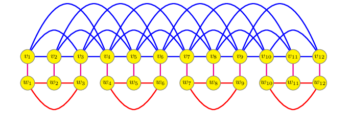
Let $B_{n}$ be the comb graph obtained by attaching one leaf at every vertex of $P_{n}$ . Now $\ell_{v}=0$ for every leaf $v$ of $B_{n}$ , and $\ell_{w}=1$ for every other vertex $w$ of $B_{n}$ , except for the two vertices $x$ and $y$ indicated in Figure 7, for which $\ell_{x}=\ell_{y}=2$ . Thus $\beta(B_{n})=2$ by Equation (16). Since $B_{n}$ has $n$ leaves, we have $\psi(B_{n})=n$ by Lemma 9.1. Moreover, $\beta(B_{n}\,\square\,B_{n})\geq n$ by Lemma 9.2. The upper bound $\beta(B_{n}\,\square\,B_{n})\leq n+1$ follows from Theorem 4.1.∎

Given that the proof of Theorem 9.3 is heavily dependent on the presence of leaves in $B_{n}$ , it is tempting to suspect that such behaviour does not occur among more highly connected graphs. This is not the case.

Theorem 9.4.

For all $k\geq 1$ and $n\geq 2$ there is a $k$ -connected graph $G_{n,k}$ for which $\beta(G_{n,k})\leq 2k$ and $\beta(G_{n,k}\,\square\,G_{n,k})\geq n$ .

Proof.

As illustrated in Figure 8, let $G_{n,k}$ be the graph with vertex set $\{v_{i},w_{i}:1\leq i\leq 2kn\}$ , where every $v_{i}w_{i}$ is an edge, $v_{i}v_{j}$ is an edge whenever $|i-j|\leq k$ , and $w_{i}w_{j}$ is an edge whenever $\lceil i/k\rceil=\lceil j/k\rceil$ . Note that $G_{n,1}=B_{2n}$ . Clearly $G_{n,k}$ is $k$ -connected. It is easily seen that $\{v_{i},v_{2kn+1-i}:1\leq i\leq k\}$ resolves $G_{n,k}$ . Thus $\beta(G_{n,k})\leq 2k$ .

Say $S$ doubly resolves $G_{n,k}$ . On the contrary, suppose that

S\cap\{w_{\ell k+1},w_{\ell k+2},\dots,w_{\ell k+k}\}=\emptyset

for some $\ell$ with $0\leq\ell\leq 2n-1$ . This implies that $d(w_{\ell k+1},x)=d(v_{\ell k+1},x)+1$ for every vertex $x\in S$ . Hence $S$ does not doubly resolve $w_{\ell k+1}$ and $v_{\ell k+1}$ . This contradiction proves that $S\cap\{w_{\ell k+1},w_{\ell k+2},\dots,w_{\ell k+k}\}\neq\emptyset$ for every $\ell$ with $0\leq\ell\leq 2n-1$ . Thus $|S|\geq 2n$ and $\psi(G_{n,k})\geq 2n$ . That $\beta(G_{n,k}\,\square\,G_{n,k})\geq n$ follows from Lemma 4.2.∎

We conclude that for all $k\geq 1$ , there is no function $f$ such that $\beta(G\,\square\,H)\leq f(\beta(G),\beta(H))$ for all $k$ -connected graphs $G$ and $H$ .

References

Alon et al. [1996] Noga Alon, Dmitry N. Kozlov, and Van H. Vu. The geometry of coin-weighing problems. In Proc. 37th Annual Symposium on Foundations of Computer Science (FOCS ’96), pp. 524–532. IEEE, 1996.
Beerliova et al. [pear] Zuzana Beerliova, Felix Eberhard, Thomas Erlebach, Alexander Hall, Michael Hoffmann, Matus Mihalak, and L. Shankar Ram. Network discovery and verification. In Proc. 31st Workshop on Graph Theoretic Concepts in Computer Science (WG’05), vol. 3787 of Lecture Notes in Comput. Sci., Springer, to appear.
Bogomolny and Greenwell [1999] Alex Bogomolny and Don Greenwell. Cut the knot: Invitation to Mastermind, 1999. http://www.maa.org/editorial/knot/Mastermind.html.
Brigham et al. [2003] Robert C. Brigham, Gary Chartrand, Ronald D. Dutton, and Ping Zhang. Resolving domination in graphs. Math. Bohem., 128(1):25–36, 2003.
Cantor [1964] David G. Cantor. Determining a set from the cardinalities of its intersections with other sets. Canad. J. Math., 16:94–97, 1964.
Cantor and Mills [1966] David G. Cantor and W. H. Mills. Determination of a subset from certain combinatorial properties. Canad. J. Math., 18:42–48, 1966.
Chappell et al. [2003] Glenn G. Chappell, John Gimbel, and Chris Hartman. Bounds on the metric and partition dimensions of a graph, 2003. http://www.cs.uaf.edu/˜chappell/papers/metric/.
Chartrand et al. [2000a] Gary Chartrand, Linda Eroh, Mark A. Johnson, and Ortrud R. Oellermann. Resolvability in graphs and the metric dimension of a graph. Discrete Appl. Math., 105(1-3):99–113, 2000a.
Chartrand et al. [2000b] Gary Chartrand, Christopher Poisson, and Ping Zhang. Resolvability and the upper dimension of graphs. Comput. Math. Appl., 39(12):19–28, 2000b.
Chartrand and Zhang [2003] Gary Chartrand and Ping Zhang. The theory and applications of resolvability in graphs. A survey. In Proc. 34th Southeastern International Conf. on Combinatorics, Graph Theory and Computing, vol. 160 of Congr. Numer., pp. 47–68. 2003.
Chvátal [1983] Vašek Chvátal. Mastermind. Combinatorica, 3(3-4):325–329, 1983.
Currie and Oellermann [2001] James Currie and Ortrud R. Oellermann. The metric dimension and metric independence of a graph. J. Combin. Math. Combin. Comput., 39:157–167, 2001.
Erdős and Rényi [1963] Paul Erdős and Alfréd Rényi. On two problems of information theory. Magyar Tud. Akad. Mat. Kutató Int. Közl., 8:229–243, 1963.
Frank and Silverman [1967] Peter Frank and Robert Silverman. Remarks on detection problems. Amer. Math. Monthly, 74:171–173, 1967.
Goddard [2003] Wayne Goddard. Static mastermind. J. Combin. Math. Combin. Comput., 47:225–236, 2003.
Goddard [2004] Wayne Goddard. Mastermind revisited. J. Combin. Math. Combin. Comput., 51:215–220, 2004.
Greenwell [2000] Don L. Greenwell. Mastermind. J. Recr. Math., 30:191–192, 1999-2000.
Guy and Nowakowski [1995] Richard K. Guy and Richard J. Nowakowski. Coin-weighing problems. Amer. Math. Monthly, 102(2):164, 1995.
Harary and Melter [1976] Frank Harary and Robert A. Melter. On the metric dimension of a graph. Ars Combinatoria, 2:191–195, 1976.
Kabatianski et al. [2000] Grigori Kabatianski, V. S. Lebedev, and J. Thorpe. The Mastermind game and the rigidity of Hamming spaces. In Proc. IEEE International Symposium on Information Theory (ISIT ’00), p. 375. IEEE, 2000.
Khuller et al. [1996] Samir Khuller, Balaji Raghavachari, and Azriel Rosenfeld. Landmarks in graphs. Discrete Appl. Math., 70(3):217–229, 1996.
Knuth [7677] Donald E. Knuth. The computer as master mind. J. Recreational Math., 9(1):1–6, 1976/77.
Lindström [1964] Bernt Lindström. On a combinatory detection problem. I. Magyar Tud. Akad. Mat. Kutató Int. Közl., 9:195–207, 1964.
Lindström [1965] Bernt Lindström. On a combinatorial problem in number theory. Canad. Math. Bull., 8:477–490, 1965.
Lindström [1966] Bernt Lindström. On a combinatory detection problem. II. Studia Sci. Math. Hungar, 1:353–361, 1966.
Mow [1997] Wai Ho Mow. Multiuser coding based on detecting matrices for synchronous-CDMA systems. In Proc. Cryptography and Coding, vol. 1355 of Lecture Notes in Comput. Sci., pp. 251–257. Springer, 1997.
Pippenger [1977] Nicholas Pippenger. An information-theoretic method in combinatorial theory. J. Combinatorial Theory Ser. A, 23(1):99–104, 1977.
Poisson and Zhang [2002] Christopher Poisson and Ping Zhang. The metric dimension of unicyclic graphs. J. Combin. Math. Combin. Comput., 40:17–32, 2002.
Saenpholphat and Zhang [2003] Varaporn Saenpholphat and Ping Zhang. Connected resolvability of graphs. Czechoslovak Math. J., 53(128)(4):827–840, 2003.
Saenpholphat and Zhang [2004a] Varaporn Saenpholphat and Ping Zhang. Conditional resolvability in graphs: a survey. Int. J. Math. Math. Sci., (37-40):1997–2017, 2004a.
Saenpholphat and Zhang [2004b] Varaporn Saenpholphat and Ping Zhang. Detour resolvability of graphs. In Proc. of 35th Southeastern International Conf. on Combinatorics, Graph Theory and Computing, vol. 169, pp. 3–21. 2004b.
Saenpholphat and Zhang [2004c] Varaporn Saenpholphat and Ping Zhang. On connected resolving decompositions in graphs. Czechoslovak Math. J., 54(129)(3):681–696, 2004c.
Sebő and Tannier [2004] András Sebő and Eric Tannier. On metric generators of graphs. Math. Oper. Res., 29(2):383–393, 2004.
Shanmukha et al. [2002] B. Shanmukha, B. Sooryanarayana, and K. S. Harinath. Metric dimension of wheels. Far East J. Appl. Math., 8(3):217–229, 2002.
Slater [1975] Peter J. Slater. Leaves of trees. In Proc. 6th Southeastern Conf. on Combinatorics, Graph Theory, and Computing, vol. 14 of Congressus Numerantium, pp. 549–559. 1975.
Slater [1988] Peter J. Slater. Dominating and reference sets in a graph. J. Math. Phys. Sci., 22(4):445–455, 1988.
Söderberg and Shapiro [1963] Staffan Söderberg and Harold S. Shapiro. A combinatory detection problem. Amer. Math. Monthly, 70:1066, 1963.
Sooryanarayana [1998] B. Sooryanarayana. On the metric dimension of a graph. Indian J. Pure Appl. Math., 29(4):413–415, 1998.
Sooryanarayana and Shanmukha [2001] B. Sooryanarayana and B. Shanmukha. A note on metric dimension. Far East J. Appl. Math., 5(3):331–339, 2001.
Yushmanov [1987] S. V. Yushmanov. Estimates for the metric dimension of a graph in terms of the diameters and the number of vertices. Vestnik Moskov. Univ. Ser. I Mat. Mekh., 103:68–70, 1987.

On the Metric Dimension of Cartesian Products of GraphsThanks: Research supported by projects MCYT-FEDER-BFM2003-00368, Gen-Cat-2001SGR00224, MCYT-HU2002-0010, MTM-2004-07891-C02-01, MEC-SB2003-0270, MCYT-FEDER BFM2003-00368, and Gen. Cat 2001SGR00224.

Abstract.

Key words and phrases:

2000 Mathematics Subject Classification

1. Introduction

2. Coin Weighing and Hypercubes

3. Projections

Lemma 3.1.

Proof.

Corollary 3.2.

4. Doubly Resolving Sets

Theorem 4.1.

Proof.

Lemma 4.2.

Proof.

Lemma 4.3.

Proof.

5. Complete Graphs

Lemma 5.1.

Proof.

Lemma 5.2.

Proof.

Theorem 5.3.

Proof.

6. Mastermind and Hamming Graphs

Theorem 6.1.

Lemma 6.2.

Proof.

Lemma 6.3.

Proof.

Lemma 6.4.

Proof.

Proof of Theorem 6.1.

7. Paths and Grids

Lemma 7.1.

Proof.

Lemma 7.2.

Proof.

8. Cycles

Lemma 8.1 ([21, 32]).

Lemma 8.2.

Proof.

Theorem 8.3.

Proof.

Theorem 8.4.

Proof.

Claim 8.5.

Proof.

Theorem 8.6.

Proof.

9. Trees

Lemma 9.1.

Proof.

Lemma 9.2.

Proof.

Theorem 9.3.

Proof.

Theorem 9.4.

Proof.

References

On the Metric Dimension of
Cartesian Products of GraphsThanks: Research supported by projects MCYT-FEDER-BFM2003-00368, Gen-Cat-2001SGR00224, MCYT-HU2002-0010, MTM-2004-07891-C02-01, MEC-SB2003-0270, MCYT-FEDER BFM2003-00368, and Gen. Cat 2001SGR00224.