Knots on a positive template have a boundednumber of prime factors

Michael C. Sullivan Address: Department of Mathematics (4408), Southern Illinois UniversityCarbondale, IL 62901, USA Email: msulliva@math.siu.edu

Abstract

Templates are branched 2–manifolds with semi-flows used to model “chaotic” hyperbolic invariant sets of flows on 3–manifolds. Knotted orbits on a template correspond to those in the original flow. Birman and Williams conjectured that for any given template the number of prime factors of the knots realized would be bounded. We prove a special case when the template is positive; the general case is now known to be false.

keywords

Hyperbolic flows, templates, prime knots, composite knots, positive braids

\urladdr

http://www.math.siu.edu/sullivan

\primaryclass

37D45 \secondaryclass57M25 \agt ATG Volume 5 (2005) 563–576\nlPublished: 29 June 2005

\thetitle

\theauthors

Abstract\stdspace\theabstract

AMS Classification\stdspace\theprimaryclass; \thesecondaryclass

Keywords\stdspace\thekeywords

1 Introduction

Templates are compact branched 2–manifolds with semi-flows used to model certain hyperbolic flows on 3–manifolds. Knotted orbits on a template correspond to those in the original flow. Birman and Williams conjectured that for any given template the number of prime factors of the knots realized would be bounded; see [1]. A counter example was first constructed in [8], but also see [5]. Here we prove that a for the subclass of positive templates the Birman–Williams conjecture is true. Section 2 gives background on templates; see also [6]. Section 3 reviews Cromwell’s Theorem on factoring positive braids [3]; it is our major tool. Some terminology for knots and braids is reviewed, but readers new to knot theory may want to have the text [2] on hand.

2 Templates

Templates are formed from a finite complex with two types of charts: joining charts and splitting charts, shown in Figure 1. In the joining charts the flow lines merge at a branch line. There are two entrance segments and one exit segment in the boundary. The semi-flow is tangent to the rest of the boundary. The splitting chart has one entrance segment, but its exit set is partitioned into three sub-segments, indicated by an inward curving of the middle sub-segment. The semi-flow is tangent to the two side segments. A template is formed by attaching exit sets to entrance sets. It is required that in a template the exit set consists of the middle portions of the splitting charts and that the entrance set be empty. It follows that the number of joining charts is equal to the number of splitting charts.

The invariant set of a template is the set of orbits of the semi-flow that never exit. The invariant set is the suspension (torus mapping) of a one-sided shift of finite type. (Its inverse limit is a suspended two-sided shift of finite type.) Thus, the invariant set contains infinitely many closed orbits. In a template embedded in $\mathbb{R}^{3}$ (we will always be working with a given embedding) the closed orbits form knots. These determine infinitely many knot types [4]; in some cases they support all knot types [5]. Franks and Williams [4] have shown that any template can be braided. That is any template can be isotoped so that all the closed orbits are presented as braids. If $T$ denotes a template we also use $T$ to denote the set of knot realized as periodic orbits in the semi-flow.

We define the split move via Figure 2. It changes the topology of a template but does not effect the invariant set.

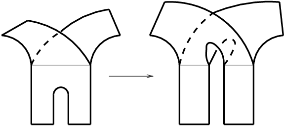
Knots can be uniquely factored (up to order) in to primes [2] – more on this in Section 3. Williams showed that the Lorenz template, which has two charts and no twisting in its bands, contains only prime knots [11]. This and other considerations led Birman and Williams [1] to conjecture that for any given template there would be a finite bound on the number of prime factors for the supported knots.

Although the original Birman–Williams Conjecture is false work in [8, 9] lead to the weakened conjecture that if a template had a braid presentation in which all crossings were of the same type, then there would be a bound on the number of prime factors of the periodic orbits. Such templates are called positive templates. This weakened Birman–Williams Conjecture is Theorem 4.1. Our major tool is a very powerful theorem on factoring positive braids due to Peter Cromwell [3].

3 Cromwell’s Factoring Theorem

Let $k$ be a knot, an embedded 1–sphere in $\mathbb{R}^{3}$ . The knot-type of $k$ is its equivalence class under ambient isotopy. An unknot or trivial knot is any knot equivalent to a circle. A projection $\pi$ of $k$ into $\mathbb{R}^{2}$ is regular if the self-intersection set of $\pi(k)$ consists of a finite number of transverse double points. We say $\pi(k)$ is irreducible if it has no cut points.

A knot $k$ is said to be factored by a 2–sphere $S$ in $\mathbb{R}^{3}$ if $k\cap S$ is transverse and consists of just two points. The factors are two knots $k_{1}$ and $k_{2}$ formed by taking the union of any simple curve on $S$ which has as end points $k\cap S$ and the portions of $k$ inside and outside of $S$ respectively. If there exists a factoring 2–sphere such that neither factor is the unknot then $k$ is a composite knot, and we write $k=k_{1}\#k_{2}$ . If the only factors of $k$ are itself and the unknot, then $k$ is prime, unless $k$ is the unknot. Schubert established that nontrivial knots can be factored uniquely into primes, up to order. An unknot can only be factored into unknots. See [2].

A smooth knot is in braid form or is braided if there is an axis with respect to which the theta derivative, in cylindrical coordinates about the axis, of some parameterization never changes sign. The regular projection onto a plane perpendicular to the axis can then be described symbolically as follows. Let $n$ be the typical number of intersection points of the projection and a radius. We say the braid has $n$ strands. We number the gaps between strands 1 to $n-1$ . Then the integers $\{-(n-1),...,-1,1,....n-1\}$ are used to specify the the order of the crossing. They determine a group under concatenation called the $B_{n}$ braid group. Thus $111$ in $B_{2}$ defines a braid with three positive crossings.

Let $B_{n}$ be the $n$ –strand braid group. A braid is positive if all its crossings are of the same type. All our braids will be positive, so we can denote a braid by a word of positive integers. Let $b=w_{1}\cdots w_{p}\in B_{n}$ , be positive. Then $b$ is decomposable if there exists positive integers $r<n$ and $q<p$ such that $w_{1},\dots,w_{q-1}$ are less then $r$ and $w_{q},\dots,w_{p}$ are greater than or equal to $r$ . E.g., $122112234343344$ is decomposable; we have $122112234343344$ = $1221122$ # $12121122$ .

Theorem 3.1 (Cromwell’s Theorem).

Let $b$ be a positive braid that is an irreducible projection of a knot $k$ . Then $k$ is prime if and only if $b$ is not decomposable.

Cromwell’s approach is to study the intersection of a would-be factoring sphere with the knot’s Seifert surface. In an unpublished note [10] Cromwell’s Theorem is proved using a template like construction. Ozawa [7] extended Cromwell’s Theorem to positive knots (knots with positive projections, but not necessarily representable as positive braids; the 5–knot is an example). Ozawa’s proof uses incompressible tori and is far more elegant than Cromwell’s original proof or that given in [10].

A factoring sphere system for a composite knot is a disjoint set of 2–spheres that factor the knot into primes. Let $k$ be a positive braid with $n$ prime factors. Then it follows from Cromwell’s Theorem that there is a factoring sphere system for $k$ which consists of $n-1$ concentric spheres meeting $\mathbb{R}^{2}$ in $n-1$ concentric circles about the braid axis. It will be convenient to allow for small deformations in the circles.

4 The Theorem

Theorem 4.1.

For any positive braided template $T$ , there exists a positive integer $N=N(T)$ , such that for every knot $k$ in $T$ , the number of prime factors of $k$ is less than or equal to $N$ .

Proof.

For a knot $k$ let $F(k)$ be the number of prime factors of $k$ . Let $T$ be a positive template with $k$ a closed orbit. Let $J$ be the number of joining charts, and $B=2J$ be the number of bands. Let $N=1+\mbox{dim}H_{1}(T)+J(1+(2J)!)(2J(1+(2J)!)-1)$ . We will show that $F(k)\leq N$ .

We specify a very nice projection of $T$ into the plane. Let $\pi:\mathbb{R}^{3}\to P\approx\mathbb{R}^{2}$ be the projection that sends $(x,y,z)$ to $(x,y,0)$ . We position $T$ in $\mathbb{R}^{3}$ so that $T$ is always in $P\times[0,\epsilon]$ and $\pi(k)$ has only transverse crossings for any $k\in T$ . (In this paragraph $k$ stands for any periodic orbit of $T$ .) Place each branch line parallel the $x$ –axis with the semi-flow coming down (decreasing $y$ ). The bands remain in $P$ with three exceptions. (i) Where a band has a half twist it will go above $P$ ( $z>0$ ) but stay within $P\times[0,\epsilon]$ and the $T$ is isotoped so that $\pi(k)$ is transverse, as in Figure 3. (ii) When two bands cross we insure that $\pi(k)$ is transverse, $T\subset P\times[0,\epsilon]$ , and we do not allow more than two bands to cross at a time. (iii) Just above (in the $y$ direction) each branch line we insure $\pi(k)$ is transverse and $T\subset P\times[0,\epsilon]$ ; see again the joining chart in Figure 1.

Suppose $k\in T$ is composite. By Cromwell’s Theorem there exists a collection of concentric topological circles in $P$ , $\mathcal{C}=\{C_{1},...,C_{n}\}$ that factor $\pi(k)$ into $n+1=F(k)$ primes; assume $C_{i}$ is interior to $C_{i+1}$ for $i=1,...,n-1$ . Let $\mathcal{S}=\{S_{i}=C_{i}\times[-i,i]\>\mbox{union two disks}\>\}_{i=1}^{n}$ . Then $\mathcal{S}$ is a complete factoring sphere system for $k$ as it appears in $T$ . We isotope the $C_{i}$ ’s so that $\mathcal{S}$ is transverse to $T$ and is still a complete factoring sphere system. Hence, $\mathcal{S}\cap T$ is compact.

Let $\beta$ be the set of branch points of $T$ . The intersection $\mathcal{S}\cap T$ determines a finite 1–complex where the vertices are the points $\mathcal{S}\cap(\partial T\cup\beta)$ . The points $\mathcal{S}\cap\partial T$ have valence one, while the points $\mathcal{S}\cap\beta$ have valence three.

The one-dimensional simplices of $\mathcal{S}\cap T$ are classified as follows. The boundary of $T$ can be partitioned into segments (one-simplices) whose end points are on the branch lines. Denote by $\partial^{0}T$ the union of those segments of $\partial T$ where the semi-flow never exits. Call the remaining segments band splitting or exit segments.

•

$\lfloor$ –segments connect a branch point to a point on $\partial^{0}T$ below and to the right.
•

$\rfloor$ –segments connect a branch point to a point on $\partial^{0}T$ below and to the left.
•

$\lceil$ –segments connect a branch point to a point on $\partial T$ above and to the right.
•

$\rceil$ –segments connect a branch point to a point on $\partial T$ above and to the left.
•

$bs$ –segments connect a branch point to a point on an exit segment.
•

$bb$ –segments, or branch-to-branch segments connect one branch line to another.
•

$ss$ –segments, or edge-to-edge segments connect one side of a band to the other.
•

$\cap$ –segments connect two points on a branch line from above.
•

$\cup$ –segments connect two points on a branch line from below.
•

$($ –segments connect two points of a segment of $\partial T$ .
•

Trivial loops are loops that miss $\partial T\cup\beta$ .

The choice of $\mathcal{C}$ and hence $\mathcal{S}$ is far from unique. We shall insist on the following minimality assumptions.

•

The number of segments in $\mathcal{S}\cap T$ is the smallest among all prime factoring sphere systems of $k$ , as constructed above.
•

The number of branch points in $\mathcal{S}\cap T$ is the smallest possible relative to the assumptions above.

Lemma 4.2.

There are no trivial loops, $($ –, $\lfloor$ –, $\rfloor$ –, $\cup$ – or $\cap$ –segments in $\mathcal{S}\cap T$ .

Proof.

If a trivial loop in $\mathcal{S}\cap T$ meets the knot $k$ then a trivial factor is produced. This is not permitted. If a trivial loop misses $k$ the corresponding sphere misses $k$ . This is not permitted. If a $($ –segment meets $k$ a trivial factor in produced. If a $($ –segment misses $k$ we may assume it is inner most and deform the corresponding sphere to eliminate it, reducing the number a segments in $\mathcal{S}\cap T$ .

For $\lfloor$ –, $\rfloor$ –, and $\cup$ –segments the arguments are similar and can be found in Lemma 1.1 of [11].

For $\cap$ –segments we consider three cases, (a), (b) and (c) as shown in Figure 4. In (a) and (b) $\pi(\mathcal{S}\cap T)$ has valence three points contradicting the fact that $\mathcal{C}$ consists of a union of simple closed curves. (We shall say that there are no Y’s in $\pi(\mathcal{S}\cap T)$ .) The configuration in (c) can be deformed to yield a factoring sphere system $\mathcal{S}^{\prime}$ with fewer segments in $\mathcal{S}^{\prime}\cap T$ , contradicting the minimality assumptions. ∎

Lemma 4.3.

The connected components of $\mathcal{S}\cap T$ consist of three types.

1.

$ss$ –segments.
2.

Nontrivial trees (trees with more than one segment).
3.

Graphs consisting of a single cycle and some $\lceil$ – or $\rceil$ –segments.

Proof.

If a component contains an $ss$ –segment, it is an $ss$ –segment. We need show that a non-tree component has only one cycle. A cycle is formed only from $bb$ –segments. Pick a vertex on a cycle. Tracing down (with the semi-flow) we must encounter a $bb$ –segment. If there are two $bb$ –segments above our vertex, then there is a Y is the projection. Thus, above the vertex there is one $bb$ –segment and either a $\lceil$ – or $\rceil$ –segment. ∎

Let $\tau$ be a non-trivial tree component in $\mathcal{S}\cap T$ . Pick a point on $\tau$ and trace down (with the flow direction). This path must exit the template somewhere. Since there are no $\rfloor$ – or $\lfloor$ –segments there must be a $bs$ –segment. (The trunk of a tree is rooted at a split.) Now trace up. When we meet a branch line we make a choice as to which segment to take. If possible we avoid $\rceil$ – and $\lceil$ –segments in favor of a $bb$ –segment. But, this path too must terminate. Therefore there is a branch line meeting $\tau$ where both of the segments above are $\rceil$ – or $\lceil$ –segments. Call this the treetop. If both segments are the same type, minimality is violated; pushing the sphere down through the branch line reduces the number of segments. Furthermore, the front one must be a $\lceil$ –segment, and the back one must be a $\rceil$ –segment or else the projection $\pi(\tau)$ will contain a Y. See Figure 5.

We use split moves to remove all tree components from $\mathcal{S}\cap T$ . Figure 6 gives an example. Of course each split move changes the number charts and bands; $J$ will increase by 1, and $B$ will increase by 2. (The number of $ss$ –segments is also increased, by 2 at a tree-top, and by 1 otherwise, per tree.) An upper bound on the number of split moves needed to remove all of the tree components for a given template $T$ can be derived from the following facts.

1.

Since a tree component projects into a braided circle it cannot meet the same branch line twice.
2.

“Parallel” trees, those that use the same bands, are removed by the same sequence of split moves. See Figure 6.
3.

The number of sets of parallel groupings of trees is bounded by $B!$ . This follows from (1).

Therefore, the maximum number of split moves needed to remove all the tree components from $T$ is $JB!$ . Call the new template formed $T^{\prime}$ .

Notation: For an oriented knot $k$ and points $a$ and $b$ on $k$ , let $k(a,b)$ denote the oriented arc in $k$ starting at $a$ and ending at $b$ .

Lemma 4.4.

The number of non-tree components is bounded by $\dim H_{1}(T)$ .

Proof.

Any cycle in $\mathcal{S}\cap T^{\prime}$ corresponds to a cycle in $\mathcal{S}\cap T$ since the split moves do not introduce new non-tree components. We will show that if $\mathcal{S}\cap T^{\prime}$ has two parallel cycles, by which we mean they pass through the same bands (they are homologous), then the factoring of $k$ by $\mathcal{S}$ produces an unknotted factor. This contradiction will give the result.

Suppose two graphs components ( $G_{1}$ , $G_{2}$ ) have parallel cycles ( $C_{1}$ , $C_{2}$ ). Assume the cycles are inner most, that is there are no other cycles in between them. Thus they bound an annulus $A$ in $T^{\prime}$ . Let $S_{1}$ and $S_{2}$ be the corresponding spheres with $S_{1}$ inside $S_{2}$ . The annulus $A$ meets only these two spheres and $A\cap\mathcal{S}=C_{1}\cup C_{2}$ . The two spheres partition $\mathbb{R}^{3}$ into three regions with the interior of $A$ in between $S_{1}$ and $S_{2}$ .

The knot $k$ pierces each sphere ( $S_{1}$ , $S_{2}$ ) exactly twice. First suppose the knot $k$ pierces each component ( $G_{1}$ , $G_{2}$ ) exactly twice. Let $k\cap G_{i}=\{p_{i},q_{i}\}$ , for $i=1,2$ . We will construct a closed loop $u$ that is a factor of $k$ . We will show that $u$ is an unknot, thus deriving a contradiction. Start from $p_{2}$ and assume without loss of generality that $k$ passes from outside $S_{2}$ to its inside.

If $k$ meets $q_{2}$ before hitting $S_{1}$ form $u$ by uniting the arc of $k$ from $p_{2}$ to $q_{2}$ with a circular arc in $C_{1}$ . Since $u$ is embedded in an annulus it is unknotted.

Assume $k$ enters $S_{1}$ at $p_{1}$ and re-emerges at $q_{1}$ . Its next intersection with $\mathcal{S}$ will be at $q_{2}$ . Form $u$ by taking the union of the arc $k(p_{2},p_{1})$ , an arc of $G_{1}$ connecting $p_{1}$ to $q_{1}$ , the arc $k(q_{1},q_{2})$ , and an arc of $G_{2}$ connecting $q_{2}$ to $p_{2}$ . We chose the arcs in $G_{1}$ and $G_{2}$ so that $u$ is braided (although we may need to make a small isotopy if these arcs start or end on $\lceil$ – or $\rceil$ –segments.) We divide the problem into subcases.

First suppose $k$ misses the annulus $A$ . Thus, $p_{1}$ , $p_{2}$ , $q_{1}$ , and $q_{2}$ are in $\lceil$ – or $\rceil$ –segments. The construction for $u$ is shown in Figure 7 where $u$ is seen to be an unknot.

Now suppose $p_{2}$ is in a $\rceil$ –segment, but that $k$ enters $A$ , say at a point $x$ on the branch line $\beta_{1}$ . Our $k$ may wind around on $A$ but will not meet $\beta_{1}$ to the left of $x$ , otherwise it could not get to $G_{1}$ . Suppose it winds around $m-1$ times before meeting $G_{1}$ . (Notice $p_{1}\in C_{1}$ .) So far $u$ has no crossings. When $k$ re-emerges from $S_{1}$ it must do so through a $\lceil$ –segment, otherwise it cannot get back to $G_{2}$ . If $k$ exits $S_{2}$ without meeting $A$ at a $\lceil$ –segment, $u$ will have braid word $m(m-1)\cdots 21$ , which is an unknot. If $k$ does re-enter $A$ , say at a point $y$ of the branch line $\beta_{2}$ , then $y$ is to the left of every point of $k(p_{2},p_{1})\cap\beta_{2}$ , otherwise $k$ will never get back to $G_{2}$ . Suppose $k(q_{1},q_{2})$ wraps around $A$ $n-1$ times before exiting $S_{2}$ . Then the braid word of $k$ is of the form $12\cdots nm(m-1)\cdots(n+1)$ ; see Figure 8. Again, $u$ is an unknot.

It may be that $k$ misses both $G_{1}$ and $G_{2}$ . In this case, $p_{1}$ , $p_{2}$ , $q_{1}$ , and $q_{2}$ are on $ss$ –segments just below and above bands that $C_{1}$ and $C_{2}$ pass through. The construction of $u$ is now very similar to the subcase above where $k$ missed the annulus $A$ . The only difference is that $u$ will have small segments on the spheres that are outside of the template. See Figure 9.

Now if $k$ enters $S_{1}$ and $S_{2}$ through $G_{1}$ and $G_{2}$ but exits through $ss$ –segments (or vise versa) it is not hard to show that $u$ will have braid word of the form $m\cdots 1$ and is thus unknotted. There are no other cases. ∎

We now turn to the $ss$ –segments in $T^{\prime}$ . Our goal is to bound the number of spheres needed to factor knots in $T$ . Thus we only need to bound the number of $ss$ –segments that meet $k$ . We classify such $ss$ –segments into two subtypes. Let $E$ be an $ss$ –segment that meets $k$ . Let $C_{i}$ be the circle containing $E$ . At some point $p$ , $k$ meets $C_{i}\cap T^{\prime}$ once again. If the component that $p$ is in is a non-tree graph, call $E$ an $ssg$ –segment. If the component that $p$ is in is another $ss$ –segment, call $E$ an $ssss$ –segment. In this case the $ss$ –segment containing $p$ is denoted $\hat{E}$ , and $E$ and $\hat{E}$ are called associated $ssss$ –segments. Clearly, the number of $ssg$ –segments is bounded by the number of non-tree components. Let $B^{\prime}$ be the number of bands in $T^{\prime}$ ; $B^{\prime}\leq B+2J(2J)!=B(1+B!)$ , since each split move produces two additional bands.

Lemma 4.5.

The number of $ssss$ –segments in $T^{\prime}$ is bounded by $B^{\prime}(B^{\prime}-1)$ .

Proof.

The proof is divided into two claims.

Claim 1\quaTwo associated $ssss$ –segments cannot be in the same band.

Let $E$ and $\hat{E}$ be associated $ssss$ –segments. Assume they are inner most among such pairs. There cannot be a segment from another circle between them. If the knot misses $E$ and $\hat{E}$ we can deform the sphere so as to reduce the number of segments by two. If the knots meet $E$ or $\hat{E}$ , it meets both, and a trivial factor is produced, as Figure 10 shows.

Let $E_{1}$ and $E_{2}$ be $ssss$ –segments in the same band $b$ . Let $\hat{E}_{1}$ and $\hat{E}_{2}$ be their respective associates.

Claim 2\quaThe segments $\hat{E}_{1}$ and $\hat{E}_{2}$ cannot be in the same band.

Suppose they were both in the band $\hat{b}$ . We can assume such a pairing is inner most. Then Figure 11 shows that a trivial factor would be produced.

The two Claims imply the desired bound holds. ∎

The lemmas above establish that $F(k)\leq N(T)$ .

References

[1] J. Birman & R. Williams. Knotted Periodic Orbits in Dynamical Systems II: Knot Holders for Fibered Knots. Contemporary Math. 20 (1983) 1–60. \MR0718132
[2] G. Burde & H. Zieschang. Knots, Second edition, de Gruyter Studies in Mathematics, 5, Walter de Gruyter & Co., Berlin, 2003. \MR1959408
[3] P. Cromwell. Positive braids are visually prime. Proc. London Math. Soc. (3) 67 (1993) 384–424. \MR1226607
[4] J. Franks & R. Williams. Entropy and knots. Trans. Amer. Math. Soc. 291 (1985), no. 1, 241–253. \MR0797057
[5] R. Ghrist. Branched two-manifolds supporting all links. Topology 36 (1997), no. 2, 423–448. \MR1415597
[6] R. Ghrist, P. Holmes & M. Sullivan. Knots and links in Three-Dimensional Flows, Lecture Notes in Mathematics, Vol. 1654, Springer-Verlag, Berlin, 1997. \MR1480169
[7] M. Ozawa. Closed incompressible surfaces in the complements of positive knots. Comment. Math. Helv. 77 (2002), no. 2, 235–243. \MR1915040
[8] M. Sullivan. Composite knots in the Figure-8 knot complement can have any number of prime factors, Top. and its Appl. 55 (1994) 261–272. \MR1259509
[9] M. Sullivan. The prime decomposition of knotted periodic orbits in dynamical systems, The Journal of Knot Theory and its Ramifications, Vol. 3 No. 1 (1994) 83-120. \MR1265454
[10] M. Sullivan. Factoring positive braids via branched manifolds. Preprint. http://galileo.math.siu.edu/~msulliva/Preprints/
[11] R. F. Williams. Lorenz Knots are Prime, Ergod. Th. & Dynam. Sys. 4 (1983) 147–163. \MR0758900

\Addresses

Received:\qua1 February 2005