跳到论文正文
W Papers独立论文阅读器 arXiv:math/0507266 论文正文 计算阅读时间 · 0%
引用这篇论文根据当前论文元数据生成,正式投稿前建议核对。


License: Assumed arXiv.org perpetual non-exclusive license
arXiv:math/0507266v2 [math.GT] 06 Nov 2006

The Magnus representation and higher-order Alexander invariants for homology cobordisms of surfaces

Takuya SAKASAI Address: Graduate School of Mathematical Sciences, the University of Tokyo, 3-8-1 Komaba, Meguro-ku, Tokyo 153-8914, Japan Email address: sakasai@ms.u-tokyo.ac.jp
Abstract.

The set of homology cobordisms from a surface to itself with markings of their boundaries has a natural monoid structure. To investigate the structure of this monoid, we define and study its Magnus representation and Reidemeister torsion invariants by generalizing Kirk-Livingston-Wang’s argument over the Gassner representation of string links. Moreover, by applying Cochran and Harvey’s framework of higher-order (non-commutative) Alexander invariants to them, we extract several pieces of information about the monoid and related objects.

Key words and phrases: 
homology cylinder; Magnus representation; higher-order Alexander invariant; string link; Dieudonné determinant; Reidemeister torsion
2000 Mathematics Subject Classification
Primary 57M05, Secondary 20F34; 57N05; 57M27

1. Introduction

Let Σg,1\Sigma_{g,1} be a compact connected oriented surface of genus g≥1g\geq 1 with one boundary component. A homology cylinder (over Σg,1\Sigma_{g,1}) consists of a homology cobordism from Σg,1\Sigma_{g,1} to itself with markings of its boundary. We denote by 𝒞g,1\mathcal{C}_{g,1} the set of isomorphisms classes of homology cylinders. Stacking two homology cylinders gives a new one, and by this, we can endow 𝒞g,1\mathcal{C}_{g,1} with a monoid structure (see Section 2 for the precise definition). The origin of homology cylinders goes back to Habiro [7], Garoufalidis-Levine [6] and Levine [14], where the clasper (or clover) surgery theory is effectively used to investigate the structure of 𝒞g,1\mathcal{C}_{g,1}.

By a standard method, we can assign a homology cylinder to each homology 3-sphere or pure string link. Also, for a given homology cylinder, we can use an element of the mapping class group of Σg,1\Sigma_{g,1} to construct another one by changing its markings. Since these operations preserve each monoid structure, 𝒞g,1\mathcal{C}_{g,1} can be regarded as a simultaneous generalization of the monoid of homology 3-spheres, that of string links and the mapping class group, any of which plays an important role in the theory of 3-manifolds. On the other hand, there exists a natural way (called closing) to construct a closed 3-manifold from each homology cylinder. Therefore, through its monoid structure, 𝒞g,1\mathcal{C}_{g,1} serves as an effective tool for classifying closed 3-manifolds.

The aim of this paper is to study the structure of 𝒞g,1\mathcal{C}_{g,1} from rather an algebraic point of view. We mainly use non-commutative rings arising from group rings to define some invariants such as the Magnus representation for 𝒞g,1\mathcal{C}_{g,1} and Reidemeister torsion invariants. Note that our Magnus representation extends that for the mapping class group defined by Morita [16], as the Gassner representation for string links due to Le Dimet [11] and Kirk-Livingston-Wang [10] does that for the pure braid group. See Birman’s book [1] for generalities of the ordinary (pre-extended) Magnus representation, including free differentials.

After defining invariants using non-commutative rings, we shall need some devices to extract information from them. For that, we use the framework of higher-order Alexander invariants due to Cochran [2] and Harvey [8, 9]. Higher-order Alexander invariants are those for finitely presentable groups interpreted as degrees of “non-commutative Alexander polynomials”, which have some unclear ambiguity except their degrees. Historically, they are first defined for knot groups by Cochran, and then generalized for arbitrary finitely presentable groups by Harvey. Using them, Cochran and Harvey obtained various sharper results than those brought by the ordinary Alexander invariants — lower bounds on the knot genus or the Thurston norm, necessary conditions for realizing a given group as the fundamental group of some compact oriented 3-manifold, and so on. In the process of applying higher-order Alexander invariants to our case, we shall give its slight generalization (called torsion-degree functions) because of the difference of localizations of non-commutative rings used in the Magnus representation and higher-order Alexander invariants. Then we use it to study several properties of our invariants and relationships between them, from which we will obtain some information about the structure of 𝒞g,1\mathcal{C}_{g,1} and related 3-manifolds.

The outline of this paper is as follows. In Section 2, we review the definition of homology cylinders as well as setting up our notation and terminology. Sections 3 and 4, which are the first main part of this paper, are devoted to define the Magnus representation and study its fundamentals, including some examples. In Section 5, we review the theory of higher-order Alexander invariants, following Harvey’s papers [8, 9], and then define its generalization. In Section 6, which is the second main part, we observe several applications of our invariants.

2. Homology cylinders

Throughout the paper, we work in PL or smooth category. Let Σg,1\Sigma_{g,1} be a compact connected oriented surface of genus g≥1g\geq 1 with one boundary component. We take a base point pp on the boundary of Σg,1\Sigma_{g,1}, and take 2​g2g loops γ1,…,γ2​g\gamma_{1},\ldots,\gamma_{2g} of Σg,1\Sigma_{g,1} as shown in Figure 1. We consider them to be an embedded bouquet R2​gR_{2g} of 2​g2g-circles tied at the base point p∈∂Σg,1p\in\partial\Sigma_{g,1}. Then R2​gR_{2g} and the boundary loop ζ\zeta of Σg,1\Sigma_{g,1} together with one 2-cell make up a standard cell decomposition of Σg,1\Sigma_{g,1}. The fundamental group π1​Σg,1\pi_{1}\Sigma_{g,1} of Σg,1\Sigma_{g,1} is isomorphic to the free group F2​gF_{2g} of rank 2​g2g generated by γ1,…,γ2​g\gamma_{1},\ldots,\gamma_{2g}, in which ζ=∏i=1g[γi,γg+i]\zeta=\prod_{i=1}^{g}[\gamma_{i},\gamma_{g+i}].

Refer to caption
Figure 1. A standard cell decomposition of Σg,1\Sigma_{g,1}

A homology cylinder (M,i+,i−)(M,i_{+},i_{-}) (over Σg,1\Sigma_{g,1}), which has its origin in Habiro [7], Garoufalidis-Levine [6] and Levine [14], consists of a compact oriented 3-manifold MM and two embeddings i+,i−:Σg,1→∂Mi_{+},i_{-}:\Sigma_{g,1}\rightarrow\partial M satisfying that

  1. (1)

    i+i_{+} is orientation-preserving and i−i_{-} is orientation-reversing,

  2. (2)

    ∂M=i+​(Σg,1)∪i−​(Σg,1)\partial M=i_{+}(\Sigma_{g,1})\cup i_{-}(\Sigma_{g,1}) and i+​(Σg,1)∩i−​(Σg,1)=i+​(∂Σg,1)=i−​(∂Σg,1)i_{+}(\Sigma_{g,1})\cap i_{-}(\Sigma_{g,1})=i_{+}(\partial\Sigma_{g,1})=i_{-}(\partial\Sigma_{g,1}),

  3. (3)

    i+|∂Σg,1=i−|∂Σg,1i_{+}\bigl|_{\partial\Sigma_{g,1}}=i_{-}\bigl|_{\partial\Sigma_{g,1}},

  4. (4)

    i+,i−:H∗​(Σg,1)→H∗​(M)i_{+},i_{-}:H_{\ast}(\Sigma_{g,1})\rightarrow H_{\ast}(M) are isomorphisms.

We denote i+​(p)=i−​(p)i_{+}(p)=i_{-}(p) by p∈∂Mp\in\partial M again and consider it to be the base point of MM. We write a homology cylinder by (M,i+,i−)(M,i_{+},i_{-}) or simply by MM.

Two homology cylinders are said to be isomorphic if there exists an orientation-preserving diffeomorphism between the underlying 3-manifolds which is compatible with the embeddings of Σg,1\Sigma_{g,1}. We denote the set of isomorphism classes of homology cylinders by 𝒞g,1\mathcal{C}_{g,1}. Given two homology cylinders M=(M,i+,i−)M=(M,i_{+},i_{-}) and N=(N,j+,j−)N=(N,j_{+},j_{-}), we can construct a new homology cylinder M⋅NM\cdot N by

M⋅N=(M∪i−∘(j+)−1N,i+,j−).M\cdot N=(M\cup_{i_{-}\circ(j_{+})^{-1}}N,i_{+},j_{-}).

Then 𝒞g,1\mathcal{C}_{g,1} becomes a monoid with the unit 1𝒞g,1:=(Σg,1×I,id×1,id×0)1_{\mathcal{C}_{g,1}}:=(\Sigma_{g,1}\times I,\mathop{\mathrm{id}}\nolimits\times 1,\mathop{\mathrm{id}}\nolimits\times 0).

From the monoid 𝒞g,1\mathcal{C}_{g,1}, we can construct the homology cobordism group ℋg,1\mathcal{H}_{g,1} of homology cylinders as in the following way. Two homology cylinders M=(M,i+,i−)M=(M,i_{+},i_{-}) and N=(N,j+,j−)N=(N,j_{+},j_{-}) are homology cobordant if there exists a compact oriented 4-manifold WW such that

  1. (1)

    ∂W=M∪(−N)/(i+​(x)=j+​(x),i−​(x)=j−​(x))x∈Σg,1\partial W=M\cup(-N)/(i_{+}(x)=j_{+}(x),\,i_{-}(x)=j_{-}(x))\quad x\in\Sigma_{g,1},

  2. (2)

    the inclusions M↪WM\hookrightarrow W, N↪WN\hookrightarrow W induce isomorphisms on the homology,

where −N-N is NN with opposite orientation. We denote by ℋg,1\mathcal{H}_{g,1} the quotient set of 𝒞g,1\mathcal{C}_{g,1} with respect to the equivalence relation of homology cobordism. The monoid structure of 𝒞g,1\mathcal{C}_{g,1} induces a group structure of ℋg,1\mathcal{H}_{g,1}. In the group ℋg,1\mathcal{H}_{g,1}, the inverse of (M,i+,i−)(M,i_{+},i_{-}) is given by (−M,i−,i+)(-M,i_{-},i_{+}).

Example 2.1.

For each element φ\varphi of the mapping class group ℳg,1\mathcal{M}_{g,1} of Σg,1\Sigma_{g,1}, we can construct a homology cylinder Mφ∈𝒞g,1M_{\varphi}\in\mathcal{C}_{g,1} by setting

Mφ:=(Σg,1×I,id×1,φ×0),M_{\varphi}:=(\Sigma_{g,1}\times I,\mathop{\mathrm{id}}\nolimits\times 1,\varphi\times 0),

where collars of i+​(Σg,1)i_{+}(\Sigma_{g,1}) and i−​(Σg,1)i_{-}(\Sigma_{g,1}) are stretched half-way along ∂Σg,1×I\partial\Sigma_{g,1}\times I. This gives injective homomorphisms ℳg,1↪𝒞g,1\mathcal{M}_{g,1}\hookrightarrow\mathcal{C}_{g,1} and ℳg,1↪ℋg,1\mathcal{M}_{g,1}\hookrightarrow\mathcal{H}_{g,1}. From this, we can regard 𝒞g,1\mathcal{C}_{g,1} and ℋg,1\mathcal{H}_{g,1} as enlargements of ℳg,1\mathcal{M}_{g,1}.

Let Nk​(G):=G/(Γk​G)N_{k}(G):=G/(\Gamma^{k}G) be the kk-th nilpotent quotient of a group GG, where we define Γ1​G=G\Gamma^{1}G=G and Γl​G=[Γl−1​G,G]\Gamma^{l}G=[\Gamma^{l-1}G,G] for l≥2l\geq 2. For simplicity, we write Nk​(X)N_{k}(X) for Nk​(π1​X)N_{k}(\pi_{1}X) where XX is a connected topological space, and write NkN_{k} for Nk​(F2​g)=Nk​(Σg,1)N_{k}(F_{2g})=N_{k}(\Sigma_{g,1}).

Let (M,i+,i−)(M,i_{+},i_{-}) be a homology cylinder. By definition, i+,i−:π1​Σg,1→π1​Mi_{+},i_{-}:\pi_{1}\Sigma_{g,1}\to\pi_{1}M are both 2-connected, namely they induce isomorphisms on the first homology groups and epimorphisms on the second homology groups. Then, by Stallings’ theorem [20], i+,i−:Nk→≅Nk​(M)i_{+},i_{-}:N_{k}\xrightarrow{\cong}N_{k}(M) are isomorphisms for each k≥2k\geq 2. Using them, we obtain a monoid homomorphism

σk:𝒞g,1⟶AutNk((M,i+,i−)↦(i+)−1∘i−).\sigma_{k}:\mathcal{C}_{g,1}\longrightarrow\mathop{\mathrm{Aut}}\nolimits N_{k}\qquad((M,i_{+},i_{-})\mapsto(i_{+})^{-1}\circ i_{-}).

It can be easily checked that σk\sigma_{k} induces a group homomorphism σk:ℋg,1→AutNk\sigma_{k}:\mathcal{H}_{g,1}\to\mathop{\mathrm{Aut}}\nolimits N_{k}. We define filtrations of 𝒞g,1\mathcal{C}_{g,1} and ℋg,1\mathcal{H}_{g,1} by

𝒞g,1​[1]:=𝒞g,1,𝒞g,1​[k]:=Ker(𝒞g,1→σkAutNk)​for k≥2,ℋg,1​[1]:=ℋg,1,ℋg,1​[k]:=Ker(ℋg,1→σkAutNk)​for k≥2.\begin{array}[]{ll}\mathcal{C}_{g,1}[1]:=\mathcal{C}_{g,1},&\mathcal{C}_{g,1}[k]:=\mathop{\mathrm{Ker}}\nolimits\left(\mathcal{C}_{g,1}\xrightarrow{\sigma_{k}}\mathop{\mathrm{Aut}}\nolimits N_{k}\right)\ \mbox{for $k\geq 2$},\\ \mathcal{H}_{g,1}[1]:=\mathcal{H}_{g,1},&\mathcal{H}_{g,1}[k]:=\mathop{\mathrm{Ker}}\nolimits\left(\mathcal{H}_{g,1}\xrightarrow{\sigma_{k}}\mathop{\mathrm{Aut}}\nolimits N_{k}\right)\ \mbox{for $k\geq 2$}.\end{array}

3. The Magnus representation for homology cylinders

We first summarize our notation. For a matrix AA with entries in a ring RR, and a ring homomorphism φ:R→R′\varphi:R\to R^{\prime}, we denote by Aφ{}^{\varphi}A the matrix obtained from AA by applying φ\varphi to each entry. ATA^{T} denotes the transpose of AA. When R=ℤ​GR=\mathbb{Z}G for a group GG or its right field of fractions (if exists), we denote by A¯\overline{A} the matrix obtained from AA by applying the involution induced from (x↦x−1,x∈G)(x\mapsto x^{-1},\ x\in G) to each entry.

For a module MM, we write MnM^{n} and MnM_{n} for the modules of column and row vectors with nn entries respectively.

For a finite cell complex XX and its regular covering XΓX_{\Gamma} with respect to a homomorphism π1​X→Γ\pi_{1}X\to\Gamma, Γ\Gamma acts on XΓX_{\Gamma} from the right through its deck transformation group. Therefore we regard the ℤ​Γ\mathbb{Z}\Gamma-cellular chain complex C∗​(XΓ)C_{\ast}(X_{\Gamma}) of XΓX_{\Gamma} as a collection of free right ℤ​Γ\mathbb{Z}\Gamma-modules consisting of column vectors together with differentials given by left multiplications of matrices. For each ℤ​Γ\mathbb{Z}\Gamma-bimodule AA, the twisted chain complex C∗​(X,A)C_{\ast}(X;A) is given by the tensor product of the right ℤ​Γ\mathbb{Z}\Gamma-module C∗​(XΓ)C_{\ast}(X_{\Gamma}) and the left ℤ​Γ\mathbb{Z}\Gamma-module AA, so that C∗​(X,A)C_{\ast}(X;A) and H∗​(X,A)H_{\ast}(X;A) are right ℤ​Γ\mathbb{Z}\Gamma-modules.

3.1. Definition of the Magnus representation for homology cylinders

In what follows, we fix an integer k≥2k\geq 2, which corresponds to the class of the nilpotent quotient. The following construction is based on Kirk-Livingston-Wang’s work of the Gassner representation for string links in [10].

Let (M,i+,i−)∈𝒞g,1(M,i_{+},i_{-})\in\mathcal{C}_{g,1} be a homology cylinder. By Stallings’ theorem, NkN_{k} and Nk​(M)N_{k}(M) are isomorphic. Since NkN_{k} is a finitely generated torsion-free nilpotent group for each k≥2k\geq 2, we can embed ℤ​Nk\mathbb{Z}N_{k} into the right field of fractions 𝒦Nk:=ℤ​Nk​(ℤ​Nk−{0})−1\mathcal{K}_{N_{k}}:=\mathbb{Z}N_{k}(\mathbb{Z}N_{k}-\{0\})^{-1}. (See Section 5.) Similarly, we have ℤ​Nk​(M)↪𝒦Nk​(M):=ℤ​Nk​(M)​(ℤ​Nk​(M)−{0})−1\mathbb{Z}N_{k}(M)\hookrightarrow\mathcal{K}_{N_{k}(M)}:=\mathbb{Z}N_{k}(M)(\mathbb{Z}N_{k}(M)-\{0\})^{-1}. We consider the fields 𝒦Nk\mathcal{K}_{N_{k}} and 𝒦Nk​(M)\mathcal{K}_{N_{k}(M)} to be local coefficient systems on Σg,1\Sigma_{g,1} and MM respectively.

By a standard argument using covering spaces (see for instance [10, Proposition 2.1], [18, Lemma 5.11]), we have the following.

Lemma 3.1.

i±:H∗​(Σg,1,p,i±∗​𝒦Nk​(M))→H∗​(M,p,𝒦Nk​(M))i_{\pm}:H_{\ast}(\Sigma_{g,1},p;i_{\pm}^{\ast}\mathcal{K}_{N_{k}(M)})\to H_{\ast}(M,p;\mathcal{K}_{N_{k}(M)}) are isomorphisms as right 𝒦Nk​(M)\mathcal{K}_{N_{k}(M)}-vector spaces.

Remark 3.2.

The same conclusion as in Lemma 3.1 can be drawn for the homology with coefficients in any ℤ​π1​(M)\mathbb{Z}\pi_{1}(M)-algebra AA satisfying the following property: Every matrix with entries in ℤ​π1​(M)\mathbb{Z}\pi_{1}(M) sent to an invertible one by the augmentation map ℤ​π1​(M)→ℤ\mathbb{Z}\pi_{1}(M)\to\mathbb{Z} is also invertible in AA. Note that 𝒦Nk​(M)\mathcal{K}_{N_{k}(M)} satisfies this property.

Since R2​g⊂Σg,1R_{2g}\subset\Sigma_{g,1} is a deformation retract, we have

H1​(Σg,1,p,i±∗​𝒦Nk​(M))≅H1​(R2​g,p,i±∗​𝒦Nk​(M))=C1​(R2​g~)⊗π1​R2​gi±∗​𝒦Nk​(M)≅𝒦Nk​(M)2​gH_{1}(\Sigma_{g,1},p;i_{\pm}^{\ast}\mathcal{K}_{N_{k}(M)})\cong H_{1}(R_{2g},p;i_{\pm}^{\ast}\mathcal{K}_{N_{k}(M)})=C_{1}(\widetilde{R_{2g}})\otimes_{\pi_{1}R_{2g}}i_{\pm}^{\ast}\mathcal{K}_{N_{k}(M)}\cong\mathcal{K}_{N_{k}(M)}^{2g}

with a basis

{γ1~⊗1,…,γ2​g~⊗1}⊂C1​(R2​g~)⊗π1​R2​gi±∗​𝒦Nk​(M)\{\widetilde{\gamma_{1}}\otimes 1,\ldots,\widetilde{\gamma_{2g}}\otimes 1\}\subset C_{1}(\widetilde{R_{2g}})\otimes_{\pi_{1}R_{2g}}i_{\pm}^{\ast}\mathcal{K}_{N_{k}(M)}

as a right 𝒦Nk​(M)\mathcal{K}_{N_{k}(M)}-vector space, where γi~\widetilde{\gamma_{i}} is a lift of γi\gamma_{i} on the universal covering R2​g~\widetilde{R_{2g}}.

Definition 3.3.

(1)(1) For each M=(M,i+,i−)∈𝒞g,1M=(M,i_{+},i_{-})\in\mathcal{C}_{g,1}, we denote by rk′​(M)∈G​L​(2​g,𝒦Nk​(M))r^{\prime}_{k}(M)\in GL(2g,\mathcal{K}_{N_{k}(M)}) the representation matrix of the right 𝒦Nk​(M)\mathcal{K}_{N_{k}(M)}-isomorphism

𝒦Nk​(M)2​g≅H1​(Σg,1,p,i−∗​𝒦Nk​(M))→i−≅H1​(M,p,𝒦Nk​(M))→i+−1≅H1​(Σg,1,p,i+∗​𝒦Nk​(M))≅𝒦Nk​(M)2​g\mathcal{K}_{N_{k}(M)}^{2g}\cong H_{1}(\Sigma_{g,1},p;i_{-}^{\ast}\mathcal{K}_{N_{k}(M)})\xrightarrow[i_{-}]{\cong}H_{1}(M,p;\mathcal{K}_{N_{k}(M)})\xrightarrow[i_{+}^{-1}]{\cong}H_{1}(\Sigma_{g,1},p;i_{+}^{\ast}\mathcal{K}_{N_{k}(M)})\cong\mathcal{K}_{N_{k}(M)}^{2g}

(2)(2) The Magnus representation for 𝒞g,1\mathcal{C}_{g,1} is the map rk:𝒞g,1→G​L​(2​g,𝒦Nk)r_{k}:\mathcal{C}_{g,1}\to GL(2g,\mathcal{K}_{N_{k}}) which assigns to M=(M,i+,i−)∈𝒞g,1M=(M,i_{+},i_{-})\in\mathcal{C}_{g,1} the matrix rk′i+−1​(M){}^{i_{+}^{-1}}r^{\prime}_{k}(M).

While we call rk​(M)r_{k}(M) the Magnus “representation”, it is actually a crossed homomorphism, namely we have the following.

Theorem 3.4.

For M1,M2∈𝒞g,1M_{1},M_{2}\in\mathcal{C}_{g,1}, we have

rk​(M1⋅M2)=rk​(M1)⋅rkσk​(M1)​(M2).r_{k}(M_{1}\cdot M_{2})=r_{k}(M_{1})\cdot{}^{\sigma_{k}(M_{1})}r_{k}(M_{2}).
Proof.

We write M=M1⋅M2M=M_{1}\cdot M_{2} for simplicity. Let i:M1→Mi:M_{1}\to M and j:M2→Mj:M_{2}\to M be the natural inclusions. Since M=(M,i∘i+,j∘j−)M=(M,i\circ i_{+},j\circ j_{-}) and i∘i−=j∘j+i\circ i_{-}=j\circ j_{+}, the map

H1​(Σg,1,p,j−∗​j∗​𝒦Nk​(M))→j∘j−H1​(M,p,𝒦Nk​(M))→(i∘i+)−1H1​(Σg,1,p,i+∗​i∗​𝒦Nk​(M))H_{1}(\Sigma_{g,1},p;j_{-}^{\ast}j^{\ast}\mathcal{K}_{N_{k}(M)})\xrightarrow{j\circ j_{-}}H_{1}(M,p;\mathcal{K}_{N_{k}(M)})\xrightarrow{(i\circ i_{+})^{-1}}H_{1}(\Sigma_{g,1},p;i_{+}^{\ast}i^{\ast}\mathcal{K}_{N_{k}(M)})

is given as the composite of

H1​(Σg,1,p,j−∗​j∗​𝒦Nk​(M))→j−H1​(M2,p,j∗​𝒦Nk​(M))→j+−1H1​(Σg,1,p,j+∗​j∗​𝒦Nk​(M))H_{1}(\Sigma_{g,1},p;j_{-}^{\ast}j^{\ast}\mathcal{K}_{N_{k}(M)})\xrightarrow{j_{-}}H_{1}(M_{2},p;j^{\ast}\mathcal{K}_{N_{k}(M)})\xrightarrow{j_{+}^{-1}}H_{1}(\Sigma_{g,1},p;j_{+}^{\ast}j^{\ast}\mathcal{K}_{N_{k}(M)})

and

H1​(Σg,1,p,i−∗​i∗​𝒦Nk​(M))→i−H1​(M1,p,i∗​𝒦Nk​(M))→i+−1H1​(Σg,1,p,i+∗​i∗​𝒦Nk​(M)).H_{1}(\Sigma_{g,1},p;i_{-}^{\ast}i^{\ast}\mathcal{K}_{N_{k}(M)})\xrightarrow{i_{-}}H_{1}(M_{1},p;i^{\ast}\mathcal{K}_{N_{k}(M)})\xrightarrow{i_{+}^{-1}}H_{1}(\Sigma_{g,1},p;i_{+}^{\ast}i^{\ast}\mathcal{K}_{N_{k}(M)}).

Hence

rk′​(M)=rk′i​(M1)⋅rk′j​(M2)⟹rk′(i​i+)−1​(M)=rk′(i​i+)−1​i​(M1)⋅rk′(i​i+)−1​j​(M2)=rk′i+−1​(M1)⋅rk′i+−1​i−1​j​(M2)=rk′i+−1​(M1)⋅rk′i+−1​i−​j+−1​(M2)⟹rk​(M)=rk​(M1)⋅rkσk​(M1)​(M2)\begin{array}[]{crcl}&r^{\prime}_{k}(M)&=&{}^{i}r^{\prime}_{k}(M_{1})\cdot{}^{j}r^{\prime}_{k}(M_{2})\\ \Longrightarrow&{}^{(i\,i_{+})^{-1}}r^{\prime}_{k}(M)&=&{}^{(i\,i_{+})^{-1}i}r^{\prime}_{k}(M_{1})\cdot{}^{(i\,i_{+})^{-1}j}r^{\prime}_{k}(M_{2})\\ &&=&{}^{i_{+}^{-1}}r^{\prime}_{k}(M_{1})\cdot{}^{i_{+}^{-1}i^{-1}j}r^{\prime}_{k}(M_{2})\\ &&=&{}^{i_{+}^{-1}}r^{\prime}_{k}(M_{1})\cdot{}^{i_{+}^{-1}i_{-}j_{+}^{-1}}r^{\prime}_{k}(M_{2})\\ \Longrightarrow&r_{k}(M)&=&r_{k}(M_{1})\cdot{}^{\sigma_{k}(M_{1})}r_{k}(M_{2})\end{array}

This completes the proof. ∎

Theorem 3.5.

rk:𝒞g,1→G​L​(2​g,𝒦Nk)r_{k}:\mathcal{C}_{g,1}\rightarrow GL(2g,\mathcal{K}_{N_{k}}) factors through ℋg,1\mathcal{H}_{g,1}.

Proof.

Suppose M1=(M1,i+,i−)M_{1}=(M_{1},i_{+},i_{-}) and M2=(M2,j+,j−)∈𝒞g,1M_{2}=(M_{2},j_{+},j_{-})\in\mathcal{C}_{g,1} are homology cobordant by a homology cobordism WW. Let i:M1→Wi:M_{1}\to W, j:M2→Wj:M_{2}\to W be the natural inclusions. We may assume that M1∪M2M_{1}\cup M_{2} is a subcomplex of WW and that WW has only one 0-cell pp. Since ℤ​Nk≅ℤ​Nk​(W)\mathbb{Z}N_{k}\cong\mathbb{Z}N_{k}(W) by Stallings’ theorem, we have 𝒦Nk​(W):=ℤ​Nk​(W)​(ℤ​Nk​(W)−{0})−1\mathcal{K}_{N_{k}(W)}:=\mathbb{Z}N_{k}(W)(\mathbb{Z}N_{k}(W)-\{0\})^{-1}. We write I+:=i∘i+=j∘j+I_{+}:=i\circ i_{+}=j\circ j_{+} and I−:=i∘i−=j∘j−I_{-}:=i\circ i_{-}=j\circ j_{-}. Then we have the following commutative diagram:

H1​(Σg,1,p,i−∗​i∗​𝒦Nk​(W))=H1​(Σg,1,p,I−∗​𝒦Nk​(W))=H1​(Σg,1,p,j−∗​j∗​𝒦Nk​(W))i−↓≅I−↓≅j−↓≅H1​(M1,p,i∗​𝒦Nk​(W))→≅iH1​(W,p,𝒦Nk​(W))←≅jH1​(M2,p,j∗​𝒦Nk​(W))(i+)−1↓≅(I+)−1↓≅(j+)−1↓≅H1​(Σg,1,p,i+∗​i∗​𝒦Nk​(W))=H1​(Σg,1,p,I+∗​𝒦Nk​(W))=H1​(Σg,1,p,j+∗​j∗​𝒦Nk​(W))\begin{CD}H_{1}(\Sigma_{g,1},p;i_{-}^{\ast}i^{\ast}\mathcal{K}_{N_{k}(W)})=H_{1}(\Sigma_{g,1},p;I_{-}^{\ast}\mathcal{K}_{N_{k}(W)})=H_{1}(\Sigma_{g,1},p;j_{-}^{\ast}j^{\ast}\mathcal{K}_{N_{k}(W)})\\ @V{i_{-}}V{\cong}V@V{I_{-}}V{\cong}V@V{j_{-}}V{\cong}V\\ H_{1}(M_{1},p;i^{\ast}\mathcal{K}_{N_{k}(W)})@>{i}>{\cong}>H_{1}(W,p;\mathcal{K}_{N_{k}(W)})@<{j}<{\cong}<H_{1}(M_{2},p;j^{\ast}\mathcal{K}_{N_{k}(W)})\\ @V{(i_{+})^{-1}}V{\cong}V@V{(I_{+})^{-1}}V{\cong}V@V{(j_{+})^{-1}}V{\cong}V\\ H_{1}(\Sigma_{g,1},p;i_{+}^{\ast}i^{\ast}\mathcal{K}_{N_{k}(W)})=H_{1}(\Sigma_{g,1},p;I_{+}^{\ast}\mathcal{K}_{N_{k}(W)})=H_{1}(\Sigma_{g,1},p;j_{+}^{\ast}j^{\ast}\mathcal{K}_{N_{k}(W)})\end{CD}

The left vertical maps give rk′i​(M1){}^{i}r^{\prime}_{k}(M_{1}) and the right ones give rk′j​(M2){}^{j}r^{\prime}_{k}(M_{2}). Applying I+−1I_{+}^{-1}, we obtain rk​(M1)=rk​(M2)r_{k}(M_{1})=r_{k}(M_{2}). ∎

Consequently, we obtain the Magnus representation rk:ℋg,1→G​L​(2​g,𝒦Nk)r_{k}:\mathcal{H}_{g,1}\to GL(2g,\mathcal{K}_{N_{k}}), which is a crossed homomorphism. If we restrict rkr_{k} to 𝒞g,1​[k]\mathcal{C}_{g,1}[k] (resp.  ℋg,1​[k]\mathcal{H}_{g,1}[k]), it becomes a monoid (resp. group) homomorphism.

Example 3.6.

For φ∈ℳg,1↪AutF2​g\varphi\in\mathcal{M}_{g,1}\hookrightarrow\mathop{\mathrm{Aut}}\nolimits F_{2g}, we can obtain

rk​(Mφ)=(∂φ⁡(γj)∂γi)ρk¯i,j,r_{k}(M_{\varphi})=\overline{\sideset{{}^{\rho_{k}}\!}{}{\mathop{\left({\displaystyle\frac{\partial\varphi(\gamma_{j})}{\partial\gamma_{i}}}\right)}\nolimits}}_{i,j},

where ρk:ℤ​F2​g→ℤ​Nk⊂𝒦Nk\rho_{k}:\mathbb{Z}F_{2g}\to\mathbb{Z}N_{k}\subset\mathcal{K}_{N_{k}} is the natural map and ∂/∂γi\partial/\partial\gamma_{i} are free differentials. From this, we see that rkr_{k} generalizes the original Magnus representation for ℳg,1\mathcal{M}_{g,1} in [16].

3.2. Computation of the Magnus matrix

In [10], the Gassner matrix of a string link is computed from the Wirtinger presentation of the fundamental group of its exterior, which gives a finite presentation whose deficiency coincides with the number of strings. Recall that the deficiency of a finite presentation P={x1,…,xn∣r1,…,rm}P=\{x_{1},\ldots,x_{n}\mid r_{1},\ldots,r_{m}\} of a finitely presentable group GG is n−mn-m, and the deficiency of GG is the maximum of all over the deficiencies of finite presentations of GG. In our context, we do not have such a useful method in general.

Definition 3.7.

For (M,i+,i−)∈𝒞g,1(M,i_{+},i_{-})\in\mathcal{C}_{g,1}, a presentation of π1​M\pi_{1}M is said to be admissible if it is of the form

⟨i−(γ1),…,i−(γ2​g),z1,…,zl,i+(γ1),…,i+(γ2​g)∣r1,…,r2​g+l⟩.\langle i_{-}(\gamma_{1}),\ldots,i_{-}(\gamma_{2g}),z_{1},\ldots,z_{l},i_{+}(\gamma_{1}),\ldots,i_{+}(\gamma_{2g})\mid r_{1},\ldots,r_{2g+l}\rangle.

Note that there does exist an admissible presentation for each homology cylinder (M,i+,i−)(M,i_{+},i_{-}). Indeed, take a Morse function with no critical points of indices 0 and 3. Then MM can be seen as Σg,1×I\Sigma_{g,1}\times I with some 1- and 2-handles. Since the Euler characteristics of Σg,1×I\Sigma_{g,1}\times I and MM are the same, the numbers of the attached 1- and 2- handles are the same. Therefore the presentation of π1​M\pi_{1}M obtained from a presentation of π1​(Σg,1×I)=F2​g\pi_{1}(\Sigma_{g,1}\times I)=F_{2g} with deficiency 2​g2g by adding new generators and relations corresponding to the 1- and 2-handles has deficiency 2​g2g again. Our claim follows from this. (See also Section 6.2.)

Given an admissible presentation of π1​M\pi_{1}M as in Definition 3.7, we define 2​g×(2​g+l)2g\times(2g+l), l×(2​g+l)l\times(2g+l) and 2​g×(2​g+l)2g\times(2g+l) matrices A,B,CA,B,C by

A=(∂rj∂i−​(γi))¯1≤i≤2​g1≤j≤2​g+l,B=(∂rj∂zi)¯1≤i≤l1≤j≤2​g+l,C=(∂rj∂i+​(γi))¯1≤i≤2​g1≤j≤2​g+lA=\overline{\left(\frac{\partial r_{j}}{\partial i_{-}(\gamma_{i})}\right)}_{\begin{subarray}{c}{}1\leq i\leq 2g\\ 1\leq j\leq 2g+l\end{subarray}},\quad B=\overline{\left(\frac{\partial r_{j}}{\partial z_{i}}\right)}_{\begin{subarray}{c}{}1\leq i\leq l\\ 1\leq j\leq 2g+l\end{subarray}},\quad C=\overline{\left(\frac{\partial r_{j}}{\partial i_{+}(\gamma_{i})}\right)}_{\begin{subarray}{c}{}1\leq i\leq 2g\\ 1\leq j\leq 2g+l\end{subarray}}

at ℤ​Nk​(M)\mathbb{Z}N_{k}(M), namely we apply the natural map

ℤ⁡⟨i−​(γ1),…,i−​(γ2​g),z1,…,zl,i+​(γ1),…,i+​(γ2​g)⟩→ℤ​π1​(M)→ℤ​Nk​(M)\mathbb{Z}\langle i_{-}(\gamma_{1}),\ldots,i_{-}(\gamma_{2g}),z_{1},\ldots,z_{l},i_{+}(\gamma_{1}),\ldots,i_{+}(\gamma_{2g})\rangle\to\mathbb{Z}\pi_{1}(M)\to\mathbb{Z}N_{k}(M)

to each entry of the matrices obtained by free differentials.

Proposition 3.8.

(1)(1) The square matrix (AB)\begin{pmatrix}A\\ B\end{pmatrix} is invertible as a matrix with entries in 𝒦Nk​(M)\mathcal{K}_{N_{k}(M)}.
(2)(2) As matrices with entries in 𝒦Nk​(M)\mathcal{K}_{N_{k}(M)}, we have

(rk′​(M)Z)​(AB)=−C(r^{\prime}_{k}(M)\quad Z)\begin{pmatrix}A\\ B\end{pmatrix}=-C

for some 2​g×l2g\times l matrix ZZ.

Proof.

(1) Let 𝔱:ℤ​Nk​(M)→ℤ\mathfrak{t}:\mathbb{Z}N_{k}(M)\to\mathbb{Z} be the augmentation map. (AB)𝔱⋅\sideset{{}^{\mathfrak{t}}}{}{\mathop{\left({\begin{smallmatrix}A\\ B\end{smallmatrix}}\right)}\nolimits}\!\cdot gives a presentation matrix of H1​(M)/Φ+H_{1}(M)/\Phi_{+}, where Φ+\Phi_{+} is the subgroup of H1​(M)H_{1}(M) generated by i+​(γ1),…,i+​(γ2​g)i_{+}(\gamma_{1}),\ldots,i_{+}(\gamma_{2g}). (See [4] for this fact through the concept of presentations of a pair of groups.) By definition, H1​(M)/Φ+=0H_{1}(M)/\Phi_{+}=0, and we have an exact sequence

ℤ2​g+l→(AB)𝔱⋅ℤ2​g+l→H1​(M)/Φ+=0.\begin{CD}\mathbb{Z}^{2g+l}@>{\sideset{{}^{\mathfrak{t}}}{}{\mathop{\left({\begin{smallmatrix}A\\ B\end{smallmatrix}}\right)}\nolimits}\!\cdot}>{}>\mathbb{Z}^{2g+l}@>{}>{}>H_{1}(M)/\Phi_{+}=0.\end{CD}

By the Hopfian property of ℤ2​g+l\mathbb{Z}^{2g+l}, we see that (AB)𝔱\sideset{{}^{\mathfrak{t}}}{}{\mathop{\left({\begin{smallmatrix}A\\ B\end{smallmatrix}}\right)}\nolimits} is invertible. (1) follows from this. (See Remark 3.2.)

(2) Through a standard argument using Eilenberg-MacLane spaces, we can assume that a given admissible presentation is obtained from a cell decomposition of MM. Then (ABC)⋅\left(\begin{smallmatrix}A\\ B\\ C\end{smallmatrix}\right)\!\cdot gives the boundary map C2​(M,p,𝒦Nk​(M))→∂2C1​(M,p,𝒦Nk​(M))C_{2}(M,p;\mathcal{K}_{N_{k}(M)})\xrightarrow{\partial_{2}}C_{1}(M,p;\mathcal{K}_{N_{k}(M)}). Considering the correspondence of 1-cycles, we have

(I2​g0(l,2​g)02​g)−(02​g0(l,2​g)rk′​(M))=(ABC)​X∈C1​(M,p,𝒦Nk​(M))\begin{pmatrix}I_{2g}\\ 0_{(l,2g)}\\ 0_{2g}\end{pmatrix}-\begin{pmatrix}0_{2g}\\ 0_{(l,2g)}\\ r^{\prime}_{k}(M)\end{pmatrix}=\begin{pmatrix}A\\ B\\ C\end{pmatrix}X\in C_{1}(M,p;\mathcal{K}_{N_{k}(M)})

for some matrix XX, where we write 0k0_{k} and 0(k,l)0_{(k,l)} for the zero matrices of sizes k×kk\times k and k×lk\times l respectively. (2) follows from this. ∎

Note that from (2), we have rk′​(M)=−C​(AB)−1​(I2​g0(l,2​g))r^{\prime}_{k}(M)=-C\begin{pmatrix}A\\ B\end{pmatrix}^{-1}\!\begin{pmatrix}I_{2g}\\ 0_{(l,2g)}\end{pmatrix}, namely the Magnus matrix rk′​(M)r^{\prime}_{k}(M) can be computed from any admissible presentation of π1​(M)\pi_{1}(M).

Next, we derive a formula for changing a generating system of π1​Σg,1\pi_{1}\Sigma_{g,1}. For a homology cylinder (M,i+,i−)(M,i_{+},i_{-}), we take an admissible presentation of π1​M\pi_{1}M as in Definition 3.7 and construct the matrices A,B,CA,B,C as before. Let γ1′,…,γ2​g′\gamma_{1}^{\prime},\ldots,\gamma_{2g}^{\prime} be another generating system of π1​Σg,1\pi_{1}\Sigma_{g,1}. We can take φ∈Autπ1​Σg,1\varphi\in\mathop{\mathrm{Aut}}\nolimits\pi_{1}\Sigma_{g,1} such that γi′=φ⁡(γi)\gamma_{i}^{\prime}=\varphi(\gamma_{i}) for i=1,…,2​gi=1,\ldots,2g.

Proposition 3.9.

Let rkφ​(M)r_{k}^{\varphi}(M) be the Magnus matrix corresponding to the new generating system. Then

rkφ​(M)=(∂φ⁡(γj)∂γi)¯−1​rk​(M)​(∂φ⁡(γj)∂γi)¯σk​(M).r_{k}^{\varphi}(M)=\overline{\left(\frac{\partial\varphi(\gamma_{j})}{\partial\gamma_{i}}\right)}^{-1}r_{k}(M)\sideset{{}^{\sigma_{k}(M)}\!}{}{\mathop{\overline{\left(\frac{\partial\varphi(\gamma_{j})}{\partial\gamma_{i}}\right)}}\nolimits}.
Proof.

We have the following admissible presentation of π1​M\pi_{1}M with respect to γ1′,…,γ2​g′\gamma_{1}^{\prime},\ldots,\gamma_{2g}^{\prime}:

π1​M≅⟨i−​(γ1′),…,i−​(γ2​g′),i−​(γ1),…,i−​(γ2​g),z1,…,zl,i+​(γ1),…,i+​(γ2​g),i+​(γ1′),…,i+​(γ2​g′)i−​(γ1′)​i−​(φ⁡(γ1))−1,…,i−​(γ2​g′)​i−​(φ⁡(γ2​g))−1,r1,…​r2​g+l,i+​(γ1′)​i+​(φ⁡(γ1))−1,…,i+​(γ2​g′)​i+​(φ⁡(γ2​g))−1,⟩.\pi_{1}M\cong\left\langle\begin{array}[]{c|c}\begin{array}[]{l}i_{-}(\gamma_{1}^{\prime}),\ldots,i_{-}(\gamma_{2g}^{\prime}),\\ i_{-}(\gamma_{1}),\ldots,i_{-}(\gamma_{2g}),\\ z_{1},\ldots,z_{l},\\ i_{+}(\gamma_{1}),\ldots,i_{+}(\gamma_{2g}),\\ i_{+}(\gamma_{1}^{\prime}),\ldots,i_{+}(\gamma_{2g}^{\prime})\end{array}&\begin{array}[]{l}i_{-}(\gamma_{1}^{\prime})i_{-}(\varphi(\gamma_{1}))^{-1},\ldots,i_{-}(\gamma_{2g}^{\prime})i_{-}(\varphi(\gamma_{2g}))^{-1},\\ r_{1},\ldots r_{2g+l},\\ i_{+}(\gamma_{1}^{\prime})i_{+}(\varphi(\gamma_{1}))^{-1},\ldots,i_{+}(\gamma_{2g}^{\prime})i_{+}(\varphi(\gamma_{2g}))^{-1},\end{array}\end{array}\right\rangle.

The matrices A′,B′,C′A^{\prime},B^{\prime},C^{\prime} corresponding to this presentation are given by

A′\displaystyle A^{\prime} =(I2​g0(2​g,2​g+l)02​g)\displaystyle=(I_{2g}\quad 0_{(2g,2g+l)}\quad 0_{2g})
B′\displaystyle B^{\prime} =(−(∂φ⁡(γj)∂γi)i−¯1≤i,j≤2​gA02​g0(l,2​g)B0(l,2​g)02​gC−(∂φ⁡(γj)∂γi)i+¯1≤i,j≤2​g)\displaystyle=\begin{pmatrix}-\overline{\sideset{{}^{i_{-}}\!}{}{\mathop{\left({\frac{\partial\varphi(\gamma_{j})}{\partial\gamma_{i}}}\right)}\nolimits}}_{1\leq i,j\leq 2g}&A&0_{2g}\\ 0_{(l,2g)}&B&0_{(l,2g)}\\ 0_{2g}&C&-\overline{\sideset{{}^{i_{+}}\!}{}{\mathop{\left({\frac{\partial\varphi(\gamma_{j})}{\partial\gamma_{i}}}\right)}\nolimits}}_{1\leq i,j\leq 2g}\end{pmatrix}
C′\displaystyle C^{\prime} =(02​g0(2​g,2​g+l)I2​g)\displaystyle=(0_{2g}\quad 0_{(2g,2g+l)}\quad I_{2g})

Computing −C′​(A′B′)−1​(I2​g0(4​g+l,2​g))-C^{\prime}\begin{pmatrix}A^{\prime}\\ B^{\prime}\end{pmatrix}^{-1}\!\begin{pmatrix}I_{2g}\\ 0_{(4g+l,2g)}\end{pmatrix}, we obtain the formula. ∎

4. Example: Relationship to the Gassner representation for string links

In [14], Levine gave a method for constructing homology cylinders from pure string links. By this, we can obtain many homology cylinders not belonging to the subgroup ℳg,1\mathcal{M}_{g,1}. Also, we can see a relationship between the Gassner representation for string links and our representation.

For a gg-component pure string link L⊂D2×IL\subset D^{2}\times I, we now construct a homology cylinder ML∈𝒞g,1M_{L}\in\mathcal{C}_{g,1} as follows. Consider a closed tubular neighborhood of the loops γg+1,γg+2,…,γ2​g\gamma_{g+1},\gamma_{g+2},\ldots,\gamma_{2g} in Figure 1 to be the image of an embedding ι:Dg↪Σg,1\iota:D_{g}\hookrightarrow\Sigma_{g,1} of a gg-holed disk DgD_{g} as in Figure 2.

Refer to caption
Figure 2.

Let CC be the complement of an open tubular neighborhood of LL in D2×ID^{2}\times I. For each choice of a framing of LL, a homeomorphism h:∂C→≅∂(ι⁡(Dg)×I)h:\partial C\xrightarrow{\cong}\partial(\iota(D_{g})\times I) is fixed. Then the manifold MLM_{L} obtained from Σg,1×I\Sigma_{g,1}\times I by removing ι⁡(Dg)×I\iota(D_{g})\times I and regluing CC by hh becomes a homology cylinder. This construction gives an injective monoid homomorphism ℒg→𝒞g,1\mathcal{L}_{g}\to\mathcal{C}_{g,1} from the monoid ℒg\mathcal{L}_{g} of (framed) pure string links to 𝒞g,1\mathcal{C}_{g,1}. Moreover it also induces an injective homomorphism 𝒮g→ℋg,1\mathcal{S}_{g}\to\mathcal{H}_{g,1} from the concordance group 𝒮g\mathcal{S}_{g} of (framed) pure string links to ℋg,1\mathcal{H}_{g,1}. In particular, the (smooth) knot concordance group, which coincides with 𝒮1\mathcal{S}_{1}, is embedded in ℋg,1\mathcal{H}_{g,1}. If we restrict these embeddings to the pure braid group, which is a subgroup of ℒg\mathcal{L}_{g} and 𝒮g\mathcal{S}_{g}, their images are contained in ℳg,1\mathcal{M}_{g,1}.

By the Gassner representation, we mean the crossed homomorphism rG,k:ℒg→G​L​(gCLOSE,r_{G,k}:\mathcal{L}_{g}\rightarrow GL(g, OPEN𝒦Nk​(Dg))\mathcal{K}_{N_{k}(D_{g})}) or rG,k:𝒮g→G​L​(g,𝒦Nk​(Dg))r_{G,k}:\mathcal{S}_{g}\rightarrow GL(g,\mathcal{K}_{N_{k}(D_{g})}) given by a construction similar to that in the previous section. (In [11] and [10], only rG,2r_{G,2} is treated.) Comparing methods for calculating the Gassner and Magnus representations, we obtain the following.

Theorem 4.1.

For any pure string link L∈ℒgL\in\mathcal{L}_{g}, rk​(ML)=(∗0g∗rG,k​(L)).r_{k}(M_{L})=\left(\begin{array}[]{cc}\ast&0_{g}\\ \ast&r_{G,k}(L)\end{array}\right).

We mention two remarks about this theorem. First we identify Fg=π1​DgF_{g}=\pi_{1}D_{g} with the subgroup of F2​g=π1​Σg,1F_{2g}=\pi_{1}\Sigma_{g,1} generated by γg+1,…,γ2​g\gamma_{g+1},\ldots,\gamma_{2g}. Then the maps Fg=⟨γg+1,…,γ2​g⟩F_{g}=\langle\gamma_{g+1},\ldots,\gamma_{2g}\rangle ↪F2​g↠Fg\hookrightarrow F_{2g}\twoheadrightarrow F_{g}, where the second map sends γ1,…,γg\gamma_{1},\ldots,\gamma_{g} to 11, show that Nk​(Fg)⊂NkN_{k}(F_{g})\subset N_{k} and 𝒦Nk​(Fg)⊂𝒦Nk\mathcal{K}_{N_{k}(F_{g})}\subset\mathcal{K}_{N_{k}}. Second, the embeddings ℒg↪𝒞g,1\mathcal{L}_{g}\hookrightarrow\mathcal{C}_{g,1} and 𝒮g↪ℋg,1\mathcal{S}_{g}\hookrightarrow\mathcal{H}_{g,1} have ambiguity with respect to framings. However we can check that the lower right part of rk​(ML)r_{k}(M_{L}) is independent of the framings.

Proof of Theorem 4.1.

All we have to do is to give a suitable presentation of π1​ML\pi_{1}M_{L}. We divide MLM_{L} into two parts MM and CC as follows.

We take gg points q1,…,qgq_{1},\ldots,q_{g} and gg paths ljl_{j} from the base point pp to qjq_{j} as in Figure 3.

Refer to caption
Figure 3.

Let MM be the union of Σg,1×I−Dg×I¯\overline{\Sigma_{g,1}\times I-D_{g}\times I} and 2​g2g paths i+​(lj)i_{+}(l_{j}) and i−​(lj)i_{-}(l_{j}) (j=1,…,g)(j=1,\ldots,g). Then

π1​M≅⟨i−​(γ1^),…,i−​(γg^)i+​(γ1^),…,i+​(γg^)i+​(γg+1),…,i+​(γ2​g)δ1,…,δg,i+​(γ)i+​(γ1^)=i−​(γ1^)​δ1⋮i+​(γg^)=i−​(γg^)​δg⟩\pi_{1}M\cong\left\langle\begin{array}[]{c|c}\begin{array}[]{c}i_{-}(\widehat{\gamma_{1}}),\ldots,i_{-}(\widehat{\gamma_{g}})\\ i_{+}(\widehat{\gamma_{1}}),\ldots,i_{+}(\widehat{\gamma_{g}})\\ i_{+}(\gamma_{g+1}),\ldots,i_{+}(\gamma_{2g})\\ \delta_{1},\ldots,\delta_{g},i_{+}(\gamma)\end{array}&\begin{array}[]{c}i_{+}(\widehat{\gamma_{1}})=i_{-}(\widehat{\gamma_{1}})\delta_{1}\\ \vdots\\ i_{+}(\widehat{\gamma_{g}})=i_{-}(\widehat{\gamma_{g}})\delta_{g}\end{array}\end{array}\right\rangle

where γj^=[γ1,γg+1]⋯[γj−1,γg+j−1]γj\widehat{\gamma_{j}}=[\gamma_{1},\gamma_{g+1}]\cdots[\gamma_{j-1},\gamma_{g+j-1}]\gamma_{j}, γ\gamma is the loop corresponding to the outer boundary of ι⁡(Dg)\iota(D_{g}) and δj\delta_{j} is the composite of paths i−​(lj)i_{-}(l_{j}), i−​(qj)​i+​(qj)→\overrightarrow{i_{-}(q_{j})i_{+}(q_{j})} and i+​(lj−1)i_{+}(l_{j}^{-1}). We denote by CC the complement of an open tubular neighborhood of LL in Dg×ID_{g}\times I as before.

π1C≅⟨i−(γg+1),…,i−(γ2​g),z1,…,zl,i+(γg+1),…,i+(γ2​g)∣r1,…rg+l⟩\pi_{1}C\cong\langle i_{-}(\gamma_{g+1}),\ldots,i_{-}(\gamma_{2g}),z_{1},\ldots,z_{l},i_{+}(\gamma_{g+1}),\ldots,i_{+}(\gamma_{2g})\mid r_{1},\ldots r_{g+l}\rangle

is given by the Wirtinger presentation of D×I−LD\times I-L. We glue CC to MM by using some fixed framing. Then it is easily seen that π1​(M∩C)\pi_{1}(M\cap C) is the free group generated by {i+(γg+1),…,i+(γ2​g),\{i_{+}(\gamma_{g+1}),\ldots,i_{+}(\gamma_{2g}), δ1,…,δg,i+(γ)}\delta_{1},\ldots,\delta_{g},i_{+}(\gamma)\}.

Using the above decomposition, we obtain

π1​ML≅⟨i−​(γ1^),…,i−​(γg^)i−​(γg+1),…,i−​(γ2​g)z1,…,zli+​(γ1^),…,i+​(γg^)i+​(γg+1),…,i+​(γ2​g)i+​(γ1^)=i−​(γ1^)​δ1^⋮i+​(γg^)=i−​(γg^)​δg^r1,…​rg+l⟩\pi_{1}M_{L}\cong\left\langle\begin{array}[]{c|c}\begin{array}[]{c}i_{-}(\widehat{\gamma_{1}}),\ldots,i_{-}(\widehat{\gamma_{g}})\\ i_{-}(\gamma_{g+1}),\ldots,i_{-}(\gamma_{2g})\\ z_{1},\ldots,z_{l}\\ i_{+}(\widehat{\gamma_{1}}),\ldots,i_{+}(\widehat{\gamma_{g}})\\ i_{+}(\gamma_{g+1}),\ldots,i_{+}(\gamma_{2g})\end{array}&\begin{array}[]{c}i_{+}(\widehat{\gamma_{1}})=i_{-}(\widehat{\gamma_{1}})\widehat{\delta_{1}}\\ \vdots\\ i_{+}(\widehat{\gamma_{g}})=i_{-}(\widehat{\gamma_{g}})\widehat{\delta_{g}}\\ r_{1},\ldots r_{g+l}\end{array}\end{array}\right\rangle

where δi^\widehat{\delta_{i}} are words in i−​(γg+1),…,i−​(γ2​g),z1,…,zli_{-}(\gamma_{g+1}),\ldots,i_{-}(\gamma_{2g}),z_{1},\ldots,z_{l}, i+​(γg+1),…,i+​(γ2​g)i_{+}(\gamma_{g+1}),\ldots,i_{+}(\gamma_{2g}) which depend on the framing. Rewrite the above presentation by using i+​(γj)i_{+}(\gamma_{j})’s and i−​(γj)i_{-}(\gamma_{j})’s instead of i+​(γj^)i_{+}(\widehat{\gamma_{j}})’s and i−​(γj^)i_{-}(\widehat{\gamma_{j}})’s. This process does not affect generators i−​(γg+j),zj,i+​(γg+j)i_{-}(\gamma_{g+j}),z_{j},i_{+}(\gamma_{g+j}) and relations rjr_{j}. From the resulting admissible presentation, we can compute the Magnus matrix of MLM_{L}. Then our claim follows by comparing it with the method for calculating the Gassner matrix of LL from the Wirtinger presentation of π1​C\pi_{1}C, which is given in [10]. ∎

Corollary 4.2.

ℳg,1\mathcal{M}_{g,1} is not a normal subgroup of ℋg,1\mathcal{H}_{g,1} for g≥3g\geq 3.

Proof.

In [10], they gave 3-component pure string links denoted by L5L_{5} and L6L_{6} having the condition that L5L_{5} is a pure braid, while the conjugate L6​L5​L6−1L_{6}L_{5}L_{6}^{-1} is not. To show that L6​L5​L6−1L_{6}L_{5}L_{6}^{-1} is not a pure braid, they use the fact that rG,2​(L6​L5​L6−1)r_{G,2}(L_{6}L_{5}L_{6}^{-1}) has an entry not belonging to ℤ​N2​(D3)\mathbb{Z}N_{2}(D_{3}). Then our claim follows from Theorem 4.1 with respect to this example. ∎

Example 4.3.

Let LL be a 2-component pure string link as depicted in Figure 4.
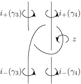
Refer to caption
Figure 4.

Then the presentation of π1​ML\pi_{1}M_{L} is given by

π1​ML≅⟨i−​(γ1),…,i−​(γ4)zi+​(γ1),…,i+​(γ4)i+​(γ1)​i−​(γ3)−1​i+​(γ4)​i−​(γ1)−1,[i+​(γ1),i+​(γ3)]​i+​(γ2)​z​i−​(γ2)−1​[i−​(γ3),i−​(γ1)],i+​(γ4)​i−​(γ3)​i+​(γ4)−1​z−1,i−​(γ3)​i+​(γ3)−1​i−​(γ3)−1​z,i−​(γ4)​z−1​i+​(γ4)−1​z,⟩,\pi_{1}M_{L}\cong\left\langle\begin{array}[]{c|c}\begin{array}[]{c}i_{-}(\gamma_{1}),\ldots,i_{-}(\gamma_{4})\\ z\\ i_{+}(\gamma_{1}),\ldots,i_{+}(\gamma_{4})\\ \end{array}&\begin{array}[]{l}i_{+}(\gamma_{1})i_{-}(\gamma_{3})^{-1}i_{+}(\gamma_{4})i_{-}(\gamma_{1})^{-1},\\ {[i_{+}(\gamma_{1}),i_{+}(\gamma_{3})]}i_{+}(\gamma_{2})zi_{-}(\gamma_{2})^{-1}{[i_{-}(\gamma_{3}),i_{-}(\gamma_{1})]},\\ i_{+}(\gamma_{4})i_{-}(\gamma_{3})i_{+}(\gamma_{4})^{-1}z^{-1},\hskip 9.24994pti_{-}(\gamma_{3})i_{+}(\gamma_{3})^{-1}i_{-}(\gamma_{3})^{-1}z,\\ i_{-}(\gamma_{4})z^{-1}i_{+}(\gamma_{4})^{-1}z,\end{array}\end{array}\right\rangle,

where we use the blackboard framing. We now compute r2​(ML)r_{2}(M_{L}). We identify N2N_{2} and N2​(ML)N_{2}(M_{L}) by using i+i_{+}. Using the presentation, we have z=i−​(γ3)=γ3z=i_{-}(\gamma_{3})=\gamma_{3}, i−​(γ4)=γ4i_{-}(\gamma_{4})=\gamma_{4}, i−​(γ2)=γ2​γ3i_{-}(\gamma_{2})=\gamma_{2}\gamma_{3} and i−​(γ1)=γ1​γ3−1​γ4i_{-}(\gamma_{1})=\gamma_{1}\gamma_{3}^{-1}\gamma_{4} in N2N_{2}. Then

(AB)\displaystyle\begin{pmatrix}A\\ B\end{pmatrix} =(−1γ3−1−10000−1000−γ1−1​γ31−γ1−1​γ3​γ4−1γ4−11−γ30000010γ2−1−1γ3γ3−γ3​γ4−1),\displaystyle=\begin{pmatrix}-1&\gamma_{3}^{-1}-1&0&0&0\\ 0&-1&0&0&0\\ -\gamma_{1}^{-1}\gamma_{3}&1-\gamma_{1}^{-1}\gamma_{3}\gamma_{4}^{-1}&\gamma_{4}^{-1}&1-\gamma_{3}&0\\ 0&0&0&0&1\\ 0&\gamma_{2}^{-1}&-1&\gamma_{3}&\gamma_{3}-\gamma_{3}\gamma_{4}^{-1}\end{pmatrix},
C\displaystyle C =(11−γ3−1000010000γ1−1−10−10γ1−1​γ301−γ3−10−γ3).\displaystyle=\begin{pmatrix}1&1-\gamma_{3}^{-1}&0&0&0\\ 0&1&0&0&0\\ 0&\gamma_{1}^{-1}-1&0&-1&0\\ \gamma_{1}^{-1}\gamma_{3}&0&1-\gamma_{3}^{-1}&0&-\gamma_{3}\end{pmatrix}.

Hence

r2​(ML)=(10000100−γ1−1γ3−1+γ4−1−1γ2−1​γ3−1​γ4−1−γ4−1+1γ3−1+γ4−1−1γ3−1γ3−1+γ4−1−1γ4−1​(γ4−1−1)γ3−1+γ4−1−1γ1−1​γ3​γ4−1γ3−1+γ4−1−1(1−γ3−1)​(γ2−1​γ3−1−γ2−1−1)γ3−1+γ4−1−1γ3−1−1γ3−1+γ4−1−1−γ3−1​γ4−1+γ3−1+2​γ4−1−1γ3−1+γ4−1−1).r_{2}(M_{L})=\left(\begin{array}[]{cccc}1&0&0&0\\ &&&\\ 0&1&0&0\\ &&&\\ \frac{-\gamma_{1}^{-1}}{\gamma_{3}^{-1}+\gamma_{4}^{-1}-1}&\frac{\gamma_{2}^{-1}\gamma_{3}^{-1}\gamma_{4}^{-1}-\gamma_{4}^{-1}+1}{\gamma_{3}^{-1}+\gamma_{4}^{-1}-1}&\frac{\gamma_{3}^{-1}}{\gamma_{3}^{-1}+\gamma_{4}^{-1}-1}&\frac{\gamma_{4}^{-1}(\gamma_{4}^{-1}-1)}{\gamma_{3}^{-1}+\gamma_{4}^{-1}-1}\\ &&&\\ \frac{\gamma_{1}^{-1}\gamma_{3}\gamma_{4}^{-1}}{\gamma_{3}^{-1}+\gamma_{4}^{-1}-1}&\frac{(1-\gamma_{3}^{-1})(\gamma_{2}^{-1}\gamma_{3}^{-1}-\gamma_{2}^{-1}-1)}{\gamma_{3}^{-1}+\gamma_{4}^{-1}-1}&\frac{\gamma_{3}^{-1}-1}{\gamma_{3}^{-1}+\gamma_{4}^{-1}-1}&\frac{-\gamma_{3}^{-1}\gamma_{4}^{-1}+\gamma_{3}^{-1}+2\gamma_{4}^{-1}-1}{\gamma_{3}^{-1}+\gamma_{4}^{-1}-1}\end{array}\right).

5. Higher-order Alexander invariants and torsion-degree functions

Here we summarize the theory of higher-order Alexander invariants along the lines of Harvey’s papers [8, 9]. For our use, we generalize them to functions of matrices called torsion-degree functions.

A group Γ\Gamma is poly-torsion-free-abelian (PTFA, for short) if Γ\Gamma has a normal series of finite length whose successive quotients are all torsion-free abelian. In particular, free nilpotent quotients NkN_{k} are PTFA for all k≥2k\geq 2. Note that every subgroup of a PTFA group is also PTFA. For each PTFA group Γ\Gamma, the group ring ℤ​Γ\mathbb{Z}\Gamma is known to be an Ore domain, so that it can be embedded in the right field of fractions 𝒦Γ:=ℤ​Γ​(ℤ​Γ−{0})−1\mathcal{K}_{\Gamma}:=\mathbb{Z}\Gamma(\mathbb{Z}\Gamma-\{0\})^{-1}, which is a skew field. We refer to [3], [17] for localizations of non-commutative rings.

We will also use the following localizations of ℤ​Γ\mathbb{Z}\Gamma placed between ℤ​Γ\mathbb{Z}\Gamma and 𝒦Γ\mathcal{K}_{\Gamma}. Let ψ:Γ↠ℤ\psi:\Gamma\twoheadrightarrow\mathbb{Z} be an epimorphism. Then we have an exact sequence

1⟶(Γψ:=Kerψ)⟶Γ⟶ψℤ⟶1.1\longrightarrow(\Gamma^{\psi}:=\mathop{\mathrm{Ker}}\nolimits\psi)\longrightarrow\Gamma\stackrel{{\scriptstyle\psi}}{{\longrightarrow}}\mathbb{Z}\longrightarrow 1.

We take a splitting ξ:ℤ→Γ\xi:\mathbb{Z}\to\Gamma and put t~:=ξ⁡(1)∈Γ\widetilde{t}:=\xi(1)\in\Gamma. Since Γψ\Gamma^{\psi} is again a PTFA group, ℤ​Γψ\mathbb{Z}\Gamma^{\psi} can be embedded in its right field of fractions 𝒦Γψ=ℤ​Γψ​(ℤ​Γψ−{0})−1\mathcal{K}_{\Gamma^{\psi}}=\mathbb{Z}\Gamma^{\psi}(\mathbb{Z}\Gamma^{\psi}-\{0\})^{-1}. Moreover, we can also construct ℤ​Γ​(ℤ​Γψ−{0})−1\mathbb{Z}\Gamma(\mathbb{Z}\Gamma^{\psi}-\{0\})^{-1}. Then the splitting ξ\xi gives an isomorphism between ℤ​Γ​(ℤ​Γψ−{0})−1\mathbb{Z}\Gamma(\mathbb{Z}\Gamma^{\psi}-\{0\})^{-1} and the skew Laurent polynomial ring 𝒦Γψ​[t±]\mathcal{K}_{\Gamma^{\psi}}[t^{\pm}], in which a​t=t⁡(t~−1​a​t~)at=t(\widetilde{t}^{-1}a\widetilde{t}\,) holds for each a∈𝒦Γψa\in\mathcal{K}_{\Gamma^{\psi}}. 𝒦Γψ​[t±]\mathcal{K}_{\Gamma^{\psi}}[t^{\pm}] is known to be a non-commutative right and left principal ideal domain. By definition, we have inclusions

ℤ​Γ↪𝒦Γψ​[t±]↪𝒦Γ.\mathbb{Z}\Gamma\hookrightarrow\mathcal{K}_{\Gamma^{\psi}}[t^{\pm}]\hookrightarrow\mathcal{K}_{\Gamma}.

𝒦Γψ​[t±]\mathcal{K}_{\Gamma^{\psi}}[t^{\pm}] and 𝒦Γ\mathcal{K}_{\Gamma} are known to be flat ℤ​Γ\mathbb{Z}\Gamma-modules. On 𝒦Γψ​[t±]\mathcal{K}_{\Gamma^{\psi}}[t^{\pm}], we have a map degψ:𝒦Γψ​[t±]→ℤ≥0∪{∞}\deg^{\psi}:\mathcal{K}_{\Gamma^{\psi}}[t^{\pm}]\to\mathbb{Z}_{\geq 0}\cup\{\infty\} assigning to each polynomial its degree. We put degψ⁡(0):=∞\deg^{\psi}(0):=\infty. By this, 𝒦Γψ​[t±]\mathcal{K}_{\Gamma^{\psi}}[t^{\pm}] becomes a Euclidean domain. The composite ℤ​Γ​(ℤ​Γψ−{0})−1→≅𝒦Γψ​[t±]→degψℤ≥0∪{∞}\mathbb{Z}\Gamma(\mathbb{Z}\Gamma^{\psi}-\{0\})^{-1}\xrightarrow{\cong}\mathcal{K}_{\Gamma^{\psi}}[t^{\pm}]\xrightarrow{\deg^{\psi}}\mathbb{Z}_{\geq 0}\cup\{\infty\} does not depend on the choice of ξ\xi.

Harvey’s higher-order Alexander invariants [9] are defined as follows. Let GG be a finitely presentable group and let φ:G↠ℤ\varphi:G\twoheadrightarrow\mathbb{Z} be an epimorphism. For a PTFA group Γ\Gamma and an epimorphism φΓ:G↠Γ\varphi_{\Gamma}:G\twoheadrightarrow\Gamma, (φΓ,φ)(\varphi_{\Gamma},\varphi) is called an admissible pair for GG if there exists an epimorphism ψ:Γ↠ℤ\psi:\Gamma\twoheadrightarrow\mathbb{Z} satisfying φ=ψ∘φΓ\varphi=\psi\circ\varphi_{\Gamma}. For each admissible pair (φΓ,φ)(\varphi_{\Gamma},\varphi) for GG, we regard 𝒦Γψ​[t±]=ℤ​Γ​(ℤ​Γψ−{0})−1\mathcal{K}_{\Gamma^{\psi}}[t^{\pm}]=\mathbb{Z}\Gamma(\mathbb{Z}\Gamma^{\psi}-\{0\})^{-1} as a ℤ​G\mathbb{Z}G-module, and we define the higher-order Alexander invariant for (φΓ,φ)(\varphi_{\Gamma},\varphi) by

δ¯Γψ​(G)\displaystyle\overline{\delta}_{\Gamma}^{\psi}(G) =dim𝒦Γψ(H1​(G,𝒦Γψ​[t±]))∈ℤ≥0∪{∞},\displaystyle=\dim_{\mathcal{K}_{\Gamma^{\psi}}}\bigl(H_{1}(G;\mathcal{K}_{\Gamma^{\psi}}[t^{\pm}])\bigr)\in\mathbb{Z}_{\geq 0}\cup\{\infty\},
δΓψ​(G)\displaystyle\delta_{\Gamma}^{\psi}(G) =dim𝒦Γψ(T𝒦Γψ​[t±]​H1​(G,𝒦Γψ​[t±]))∈ℤ≥0,\displaystyle=\dim_{\mathcal{K}_{\Gamma^{\psi}}}\bigl(T_{\mathcal{K}_{\Gamma^{\psi}}[t^{\pm}]}H_{1}(G;\mathcal{K}_{\Gamma^{\psi}}[t^{\pm}])\bigr)\in\mathbb{Z}_{\geq 0},

where T𝒦Γψ​[t±]​MT_{\mathcal{K}_{\Gamma^{\psi}}[t^{\pm}]}M denotes the 𝒦Γψ​[t±]\mathcal{K}_{\Gamma^{\psi}}[t^{\pm}]-torsion part of a 𝒦Γψ​[t±]\mathcal{K}_{\Gamma^{\psi}}[t^{\pm}]-module MM. δ¯Γψ​(G)\overline{\delta}_{\Gamma}^{\psi}(G) and δΓψ​(G)\delta_{\Gamma}^{\psi}(G) are called the Γ\Gamma-degree and the refined Γ\Gamma-degree respectively. (Our definition is slightly different from that of [9].) Note that the right 𝒦Γψ​[t±]\mathcal{K}_{\Gamma^{\psi}}[t^{\pm}]-module H1​(G,𝒦Γψ​[t±])H_{1}(G;\mathcal{K}_{\Gamma^{\psi}}[t^{\pm}]) can be decomposed into

H1​(G,𝒦Γψ​[t±])=(𝒦Γψ​[t±])r⊕(⨁i=1l𝒦Γψ​[t±]pi​(t)​𝒦Γψ​[t±])H_{1}(G;\mathcal{K}_{\Gamma^{\psi}}[t^{\pm}])=(\mathcal{K}_{\Gamma^{\psi}}[t^{\pm}])^{r}\oplus\left(\bigoplus_{i=1}^{l}\frac{\mathcal{K}_{\Gamma^{\psi}}[t^{\pm}]}{p_{i}(t)\mathcal{K}_{\Gamma^{\psi}}[t^{\pm}]}\right)

for some r∈ℤ≥0r\in\mathbb{Z}_{\geq 0} and pi​(t)∈𝒦Γψ​[t±]p_{i}(t)\in\mathcal{K}_{\Gamma^{\psi}}[t^{\pm}], then

δ¯Γψ​(G)\displaystyle\overline{\delta}_{\Gamma}^{\psi}(G) ={∑i=1ldegψ⁡(pi​(t))(r=0),∞(r>0),\displaystyle=\begin{cases}\sum_{i=1}^{l}\deg^{\psi}(p_{i}(t))&(r=0),\\ \infty&(r>0)\end{cases},
δΓψ​(G)\displaystyle\delta_{\Gamma}^{\psi}(G) =∑i=1ldegψ⁡(pi​(t)).\displaystyle=\sum_{i=1}^{l}\deg^{\psi}(p_{i}(t)).

For a connected space XX and an admissible pair (φΓ,φ)(\varphi_{\Gamma},\varphi) for π1​X\pi_{1}X, we define δ¯Γψ​(X):=δ¯Γψ​(π1​X)\overline{\delta}_{\Gamma}^{\psi}(X):=\overline{\delta}_{\Gamma}^{\psi}(\pi_{1}X) and δΓψ​(X):=δΓψ​(π1​X)\delta_{\Gamma}^{\psi}(X):=\delta_{\Gamma}^{\psi}(\pi_{1}X).

For a finitely presentable group GG and an admissible pair (φΓ,φ)(\varphi_{\Gamma},\varphi) for GG, the (refined) Γ\Gamma-degree can be computed from any presentation matrix of the right 𝒦Γψ​[t±]\mathcal{K}_{\Gamma^{\psi}}[t^{\pm}]-module H1​(G,𝒦Γψ​[t±])H_{1}(G;\mathcal{K}_{\Gamma^{\psi}}[t^{\pm}]). Therefore we can consider it to be a function on the set M⁡(𝒦Γψ​[t±])M(\mathcal{K}_{\Gamma^{\psi}}[t^{\pm}]) of all matrices with entries in 𝒦Γψ​[t±]\mathcal{K}_{\Gamma^{\psi}}[t^{\pm}]. Here we extend this function to M⁡(𝒦Γ)M(\mathcal{K}_{\Gamma}) as follows.

First, we extend degψ:𝒦Γψ​[t±]→ℤ≥0∪{∞}\deg^{\psi}:\mathcal{K}_{\Gamma^{\psi}}[t^{\pm}]\to\mathbb{Z}_{\geq 0}\cup\{\infty\} to degψ:𝒦Γ→ℤ∪{∞}\deg^{\psi}:\mathcal{K}_{\Gamma}\to\mathbb{Z}\cup\{\infty\} by setting degψ⁡(f​g−1)=degψ⁡(f)−degψ⁡(g)\deg^{\psi}(fg^{-1})=\deg^{\psi}(f)-\deg^{\psi}(g) for f∈ℤ​Γ,g∈ℤ​Γ−{0}f\in\mathbb{Z}\Gamma,g\in\mathbb{Z}\Gamma-\{0\} (see for instance [3, Proposition 9.1.1]). It induces a group homomorphism degψ:(𝒦Γ×)ab→ℤ\deg^{\psi}:(\mathcal{K}_{\Gamma}^{\times})_{\mathrm{ab}}\to\mathbb{Z}, where (𝒦Γ×)ab(\mathcal{K}_{\Gamma}^{\times})_{\mathrm{ab}} is the abelianization of the multiplicative group 𝒦Γ×=𝒦Γ−{0}\mathcal{K}_{\Gamma}^{\times}=\mathcal{K}_{\Gamma}-\{0\}.

Since 𝒦Γ\mathcal{K}_{\Gamma} is a skew field, we have the Dieudonné determinant

det:G​L​(𝒦Γ)⟶(𝒦Γ×)ab,\det:GL(\mathcal{K}_{\Gamma})\longrightarrow(\mathcal{K}_{\Gamma}^{\times})_{\mathrm{ab}},

which is a homomorphism characterized by the following three properties:

  • (a)

    detI=1\det I=1.

  • (b)

    If A′A^{\prime} is obtained by multiplying a row of a matrix A∈G​L​(𝒦Γ)A\in GL(\mathcal{K}_{\Gamma}) by a∈𝒦Γ×a\in\mathcal{K}_{\Gamma}^{\times} from the left, then detA′=a⋅detA\det A^{\prime}=a\cdot\det A.

  • (c)

    If A′A^{\prime} is obtained by adding to a row of a matrix AA a left 𝒦Γ\mathcal{K}_{\Gamma}-linear combination of other rows, then detA′=detA\det A^{\prime}=\det A.

It induces an isomorphism between K1​(𝒦Γ)→≅(𝒦Γ×)abK_{1}(\mathcal{K}_{\Gamma})\xrightarrow{\cong}(\mathcal{K}_{\Gamma}^{\times})_{\mathrm{ab}}.

The following lemma will be used in our generalization of Harvey’s invariants. We denote by M⁡(m,n,𝒦Γ)M(m,n,\mathcal{K}_{\Gamma}) the set of all m×nm\times n matrices with entries in 𝒦Γ\mathcal{K}_{\Gamma}.

Lemma 5.1.

For A∈M⁡(m,n,𝒦Γ)A\in M(m,n,\mathcal{K}_{\Gamma}) with rank𝒦ΓA=k\mathop{\mathrm{rank}}\nolimits_{\mathcal{K}_{\Gamma}}A=k, let U∈M⁡(m−k,m,𝒦Γ)U\in M(m-k,m,\mathcal{K}_{\Gamma}), V∈M⁡(n,n−k,𝒦Γ)V\in M(n,n-k,\mathcal{K}_{\Gamma}) be matrices satisfying

{U​A=0,rank𝒦ΓU=m−k,A​V=0,rank𝒦ΓV=n−k.\begin{cases}UA=0,&\mathop{\mathrm{rank}}\nolimits_{\mathcal{K}_{\Gamma}}U=m-k,\\ AV=0,&\mathop{\mathrm{rank}}\nolimits_{\mathcal{K}_{\Gamma}}V=n-k.\end{cases}

For each I⊂{1,2,…,m}I\subset\{1,2,\ldots,m\}, J⊂{1,2,…,n}J\subset\{1,2,\ldots,n\} with #​I=m−k\#I=m-k, #​J=n−k\#J=n-k, let UIU_{I} denote the square matrix defined by taking ii-th columns from UU for all i∈Ii\in I, and VJV_{J} denote the one defined by taking jj-th rows from VV for all j∈Jj\in J. We also denote by AIc​JcA_{I^{c}J^{c}} the one defined by taking ii-th rows from AA for all i∈Ic:={1,2,…,m}−Ii\in I^{c}:=\{1,2,\ldots,m\}-I and then taking jj-th columns for all j∈Jc:={1,2,…,n}−Jj\in J^{c}:=\{1,2,\ldots,n\}-J.

(1)(1) If UIU_{I} or VJV_{J} is not invertible, then AIc​JcA_{I^{c}J^{c}} is not invertible.

(2)(2) Otherwise,

Δ⁡(A,U,V):=sgn(I​Ic)​sgn(J​Jc)​detAIc​JcdetUI​detVJ∈(𝒦Γ×)ab\Delta(A;U,V):=\mathop{\mathrm{sgn}}\nolimits(II^{c})\mathop{\mathrm{sgn}}\nolimits(JJ^{c})\frac{\det A_{I^{c}J^{c}}}{\det U_{I}\det V_{J}}\in(\mathcal{K}_{\Gamma}^{\times})_{\mathrm{ab}}

is independent of the choice of II and JJ such that UIU_{I}, VJV_{J} are invertible, where sgn(I​Ic)∈{±1}\mathop{\mathrm{sgn}}\nolimits(II^{c})\in\{\pm 1\} ((resp. OPENsgn(J​Jc))\mathop{\mathrm{sgn}}\nolimits(JJ^{c})) is the signature of the juxtaposition of II and IcI^{c} ((resp. JJ and OPENJc)J^{c}), and we put det∅:=1\det\emptyset:=1.

(3)(3) For P1∈G​L​(m,𝒦Γ)P_{1}\in GL(m,\mathcal{K}_{\Gamma}), P2∈G​L​(n,𝒦Γ)P_{2}\in GL(n,\mathcal{K}_{\Gamma}), Q1∈G​L​(m−k,𝒦Γ)Q_{1}\in GL(m-k,\mathcal{K}_{\Gamma}) and Q2∈G​L​(n−k,𝒦Γ)Q_{2}\in GL(n-k,\mathcal{K}_{\Gamma}),

Δ⁡(P1−1​A​P2−1,Q1​U​P1,P2​V​Q2)=Δ⁡(A,U,V)detP1​detP2​detQ1​detQ2.\Delta(P_{1}^{-1}AP_{2}^{-1};Q_{1}UP_{1},P_{2}VQ_{2})=\frac{\Delta(A;U,V)}{\det P_{1}\det P_{2}\det Q_{1}\det Q_{2}}.
Proof.

(1) and (2) are deduced from easy observation using non-commutative linear algebra. To prove (3), it suffices to show in the cases where P1,P2,Q1,Q2P_{1},P_{2},Q_{1},Q_{2} are matrices of elementary transformations, and it can be easily checked. ∎

Remark 5.2.

In the above situation, the sequence

0→𝒦Γn−k→V⋅𝒦Γn→A⋅𝒦Γm→U⋅𝒦Γm−k→0\begin{CD}0@>{}>{}>\mathcal{K}_{\Gamma}^{n-k}@>{V\cdot}>{}>\mathcal{K}_{\Gamma}^{n}@>{A\cdot}>{}>\mathcal{K}_{\Gamma}^{m}@>{U\cdot}>{}>\mathcal{K}_{\Gamma}^{m-k}@>{}>{}>0\end{CD}

is exact. By taking the standard basis for each vector space, we regard the sequence as a based acyclic chain complex. Then we can take its torsion (see [15], [21] for generalities of torsions). This torsion coincides with Δ⁡(A,U,V)\Delta(A;U,V) up to sign.

As seen in Lemma 5.1 (3), Δ⁡(A,U,V)\Delta(A;U,V) does depend on UU and VV. The following definition and lemma give our rule to take UU and VV.

Definition 5.3.

Let A∈M⁡(m,n,𝒦Γ)A\in M(m,n,\mathcal{K}_{\Gamma}) with rank𝒦ΓA=k\mathop{\mathrm{rank}}\nolimits_{\mathcal{K}_{\Gamma}}A=k. (U,V)(U,V) is said to be ψ\psi-primitive for AA if

  • (1)

    UU, VV have entries in 𝒦Γψ​[t±]\mathcal{K}_{\Gamma^{\psi}}[t^{\pm}].

  • (2)

    The row vectors u1,…,um−k∈(𝒦Γψ​[t±])mu_{1},\ldots,u_{m-k}\in(\mathcal{K}_{\Gamma^{\psi}}[t^{\pm}])_{m} of UU generate Ker(⋅A)∩(𝒦Γψ[t±])m\mathop{\mathrm{Ker}}\nolimits(\cdot A)\cap(\mathcal{K}_{\Gamma^{\psi}}[t^{\pm}])_{m} in (𝒦Γ)m(\mathcal{K}_{\Gamma})_{m} as a left 𝒦Γψ​[t±]\mathcal{K}_{\Gamma^{\psi}}[t^{\pm}]-module.

  • (3)

    The column vectors v1,…,vn−k∈(𝒦Γψ​[t±])nv_{1},\ldots,v_{n-k}\in(\mathcal{K}_{\Gamma^{\psi}}[t^{\pm}])^{n} of VV generate Ker(A⋅)∩(𝒦Γψ[t±])n\mathop{\mathrm{Ker}}\nolimits(A\cdot)\cap(\mathcal{K}_{\Gamma^{\psi}}[t^{\pm}])^{n} in (𝒦Γ)n(\mathcal{K}_{\Gamma})^{n} as a right 𝒦Γψ​[t±]\mathcal{K}_{\Gamma^{\psi}}[t^{\pm}]-module.

Lemma 5.4.

(1)(1) There exists a pair (U,V)(U,V) which is ψ\psi-primitive for AA.
(2)(2) Suppose U∈M⁡(m−k,m,𝒦Γψ​[t±])U\in M(m-k,m,\mathcal{K}_{\Gamma^{\psi}}[t^{\pm}]) and V∈M⁡(n,n−k,𝒦Γψ​[t±])V\in M(n,n-k,\mathcal{K}_{\Gamma^{\psi}}[t^{\pm}]) satisfy U​A=0UA=0 and A​V=0AV=0. (U,V)(U,V) is ψ\psi-primitive for AA if and only if there exist P~1∈G​L​(m,𝒦Γψ​[t±])\widetilde{P}_{1}\in GL(m,\mathcal{K}_{\Gamma^{\psi}}[t^{\pm}]) and P~2∈G​L​(n,𝒦Γψ​[t±])\widetilde{P}_{2}\in GL(n,\mathcal{K}_{\Gamma^{\psi}}[t^{\pm}]) satisfying

U​P~1=(0(m−k,k)Im−k),P~2​V=(0(n−k,k)In−k)T.U\widetilde{P}_{1}=(0_{(m-k,k)}\quad I_{m-k}),\quad\widetilde{P}_{2}V=(0_{(n-k,k)}\quad I_{n-k})^{T}.

(3)(3) If (U,V)(U,V) and (U′,V′)(U^{\prime},V^{\prime}) are ψ\psi-primitive for AA, then there exist P1∈G​L​(m,𝒦Γψ​[t±])P_{1}\in GL(m,\mathcal{K}_{\Gamma^{\psi}}[t^{\pm}]), P2∈G​L​(n𝐶𝐿𝑂𝑆𝐸,P_{2}\in GL(n, 𝑂𝑃𝐸𝑁𝒦Γψ​[t±])\mathcal{K}_{\Gamma^{\psi}}[t^{\pm}]), Q1∈G​L​(m−k,𝒦Γψ​[t±])Q_{1}\in GL(m-k,\mathcal{K}_{\Gamma^{\psi}}[t^{\pm}]) and Q2∈G​L​(n−k,𝒦Γψ​[t±])Q_{2}\in GL(n-k,\mathcal{K}_{\Gamma^{\psi}}[t^{\pm}]) such that

U​P1=U′,P2​V=V′,Q1​U=U′,V​Q2=V′.UP_{1}=U^{\prime},\quad P_{2}V=V^{\prime},\quad Q_{1}U=U^{\prime},\quad VQ_{2}=V^{\prime}.
Proof.

We prove only for VV.
(1) For right 𝒦Γψ​[t±]\mathcal{K}_{\Gamma^{\psi}}[t^{\pm}]-homomorphisms (𝒦Γψ​[t±])n↪i𝒦Γn→A⋅𝒦Γm(\mathcal{K}_{\Gamma^{\psi}}[t^{\pm}])^{n}\stackrel{{\scriptstyle i}}{{\hookrightarrow}}\mathcal{K}_{\Gamma}^{n}\xrightarrow{A\cdot}\mathcal{K}_{\Gamma}^{m}, Ker((A⋅)∘i)=Ker(A⋅)∩(𝒦Γψ[t±])n\mathop{\mathrm{Ker}}\nolimits((A\cdot)\circ i)=\mathop{\mathrm{Ker}}\nolimits(A\cdot)\cap(\mathcal{K}_{\Gamma^{\psi}}[t^{\pm}])^{n} is a right free 𝒦Γψ​[t±]\mathcal{K}_{\Gamma^{\psi}}[t^{\pm}]-module of rank n−kn-k. We take a basis v1,…,vn−kv_{1},\ldots,v_{n-k} and put V=(v1,…,vn−k)V=(v_{1},\ldots,v_{n-k}). Then VV satisfies the desired property.
(2) Suppose VV generates Ker(A⋅)∩(𝒦Γψ[t±])n\mathop{\mathrm{Ker}}\nolimits(A\cdot)\cap(\mathcal{K}_{\Gamma^{\psi}}[t^{\pm}])^{n}. The quotient module (𝒦Γψ[t±])n/Ker((A⋅)∘i)(\mathcal{K}_{\Gamma^{\psi}}[t^{\pm}])^{n}/\mathop{\mathrm{Ker}}\nolimits((A\cdot)\circ i) is 𝒦Γψ​[t±]\mathcal{K}_{\Gamma^{\psi}}[t^{\pm}]-torsion free, and hence 𝒦Γψ​[t±]\mathcal{K}_{\Gamma^{\psi}}[t^{\pm}]-free. Taking a splitting, we have a direct sum decomposition (𝒦Γψ[t±])n≅((𝒦Γψ[t±])n/Ker((A⋅)∘i))⊕Ker((A⋅)∘i)(\mathcal{K}_{\Gamma^{\psi}}[t^{\pm}])^{n}\cong\bigl((\mathcal{K}_{\Gamma^{\psi}}[t^{\pm}])^{n}/\mathop{\mathrm{Ker}}\nolimits((A\cdot)\circ i)\bigr)\oplus\mathop{\mathrm{Ker}}\nolimits((A\cdot)\circ i). We can extend VV to obtain a basis (v1~,…,vk~,V)(\tilde{v_{1}},\ldots,\tilde{v_{k}},V) for (𝒦Γψ​[t±])n(\mathcal{K}_{\Gamma^{\psi}}[t^{\pm}])^{n}. Then P~2:=(v1~,…,vk~,V)−1\widetilde{P}_{2}:=(\tilde{v_{1}},\ldots,\tilde{v_{k}},V)^{-1} satisfies P~2​V=(0(n−k,k)In−k)T\widetilde{P}_{2}V=(0_{(n-k,k)}\quad I_{n-k})^{T}. The inverse is clear.
(3) The existence of P2P_{2} follows immediately from (2). That of Q2Q_{2} is also clear since VV and V′V^{\prime} are bases of the same right 𝒦Γψ​[t±]\mathcal{K}_{\Gamma^{\psi}}[t^{\pm}]-module. ∎

Definition 5.5.

Let Γ\Gamma be a PTFA group and let ψ:Γ↠ℤ\psi:\Gamma\twoheadrightarrow\mathbb{Z} be an epimorphism.
(1) The torsion-degree function dΓψ:M⁡(𝒦Γ)→ℤd_{\Gamma}^{\psi}:M(\mathcal{K}_{\Gamma})\to\mathbb{Z} is defined by

dΓψ​(A):=degψ⁡(Δ⁡(A,U,V))d_{\Gamma}^{\psi}(A):=\deg^{\psi}(\Delta(A;U,V))

for a pair (U,V)(U,V) which is ψ\psi-primitive for AA.
(2) The truncated torsion-degree function d¯Γψ:M⁡(𝒦Γ)→ℤ∪{∞}\overline{d}_{\Gamma}^{\psi}:M(\mathcal{K}_{\Gamma})\to\mathbb{Z}\cup\{\infty\} is defined by

d¯Γψ​(A):={dΓψ​(A)if rankA≥m−1,∞otherwise\overline{d}_{\Gamma}^{\psi}(A):=\begin{cases}d_{\Gamma}^{\psi}(A)&\text{if $\mathop{\mathrm{rank}}\nolimits A\geq m-1$,}\\ \infty&\text{otherwise}\end{cases}

for A∈M⁡(m,n,𝒦Γ)A\in M(m,n,\mathcal{K}_{\Gamma}).

Since 𝒦Γψ​[t±]\mathcal{K}_{\Gamma^{\psi}}[t^{\pm}] is a Euclidean domain, every P∈G​L​(𝒦Γψ​[t±])P\in GL(\mathcal{K}_{\Gamma^{\psi}}[t^{\pm}]) can be decomposed as products of elementary matrices and diagonal matrices in G​L​(𝒦Γψ​[t±])GL(\mathcal{K}_{\Gamma^{\psi}}[t^{\pm}]), which shows that degψ⁡(detP)=0\deg^{\psi}(\det P)=0. Lemmas 5.1 and 5.4 together with this fact show that dΓψd_{\Gamma}^{\psi} and d¯Γψ\overline{d}_{\Gamma}^{\psi} are well-defined.

Example 5.6.

(1) For A∈G​L​(𝒦Γ)A\in GL(\mathcal{K}_{\Gamma}), we have dΓψ​(A)=d¯Γψ​(A)=degψ⁡(detA)d_{\Gamma}^{\psi}(A)=\overline{d}_{\Gamma}^{\psi}(A)=\deg^{\psi}(\det A).
(2) Let MM be a finitely generated right 𝒦Γψ​[t±]\mathcal{K}_{\Gamma^{\psi}}[t^{\pm}]-module, and let AA be a presentation matrix of MM. Then we have dΓψ​(A)=dim𝒦Γψ(T𝒦Γψ​[t±]​M)d_{\Gamma}^{\psi}(A)=\dim_{\mathcal{K}_{\Gamma^{\psi}}}\bigl(T_{\mathcal{K}_{\Gamma^{\psi}}[t^{\pm}]}M\bigr). As for d¯Γψ​(A)\overline{d}_{\Gamma}^{\psi}(A), we can see that d¯Γψ​(A)∈ℤ\overline{d}_{\Gamma}^{\psi}(A)\in\mathbb{Z} if and only if the rank of the 𝒦Γψ​[t±]\mathcal{K}_{\Gamma^{\psi}}[t^{\pm}]-free part of MM is less than 22.
(3) Let GG be a finitely presentable group. We take a presentation ⟨x1,…,xl∣r1,…,rm⟩\langle x_{1},\ldots,x_{l}\mid r_{1},\ldots,r_{m}\rangle of GG. For an admissible pair (φΓ,φ)(\varphi_{\Gamma},\varphi), the matrix A:=(∂rj∂xi)φΓ¯1≤i≤l1≤j≤mA:=\overline{\sideset{{}^{\varphi_{\Gamma}}\!}{}{\mathop{\left({\frac{\partial r_{j}}{\partial x_{i}}}\right)}\nolimits}}_{\begin{subarray}{c}{}1\leq i\leq l\\ 1\leq j\leq m\end{subarray}} at 𝒦Γψ​[t±]\mathcal{K}_{\Gamma^{\psi}}[t^{\pm}] gives a presentation matrix of H1​(G,{1},𝒦Γψ​[t±])H_{1}(G,\{1\};\mathcal{K}_{\Gamma^{\psi}}[t^{\pm}]). Then Harvey’s invariants are given by

δΓψ​(G)\displaystyle\delta_{\Gamma}^{\psi}(G) =dim𝒦Γψ(T𝒦Γψ​[t±]​H1​(G,𝒦Γψ​[t±]))=dΓψ​(A),\displaystyle=\dim_{\mathcal{K}_{\Gamma^{\psi}}}\bigl(T_{\mathcal{K}_{\Gamma^{\psi}}[t^{\pm}]}H_{1}(G;\mathcal{K}_{\Gamma^{\psi}}[t^{\pm}])\bigr)=d_{\Gamma}^{\psi}(A),
δ¯Γψ​(G)\displaystyle\overline{\delta}_{\Gamma}^{\psi}(G) =dim𝒦Γψ(H1​(G,𝒦Γψ​[t±]))=d¯Γψ​(A),\displaystyle=\dim_{\mathcal{K}_{\Gamma^{\psi}}}\bigl(H_{1}(G;\mathcal{K}_{\Gamma^{\psi}}[t^{\pm}])\bigr)=\overline{d}_{\Gamma}^{\psi}(A),

where the second equality of each case follows from the direct sum decomposition

H1​(G,{1},𝒦Γψ​[t±])≅H1​(G,𝒦Γψ​[t±])⊕𝒦Γψ​[t±]H_{1}(G,\{1\};\mathcal{K}_{\Gamma^{\psi}}[t^{\pm}])\cong H_{1}(G;\mathcal{K}_{\Gamma^{\psi}}[t^{\pm}])\oplus\mathcal{K}_{\Gamma^{\psi}}[t^{\pm}]

shown by Harvey in [8].

Remark 5.7.

Friedl [5] gave an interpretation of Harvey’s invariants by Reidemeister torsions. The definition of our truncated torsion-degree functions has some overlaps with his description.

6. Applications of torsion-degree functions to homology cylinders

In this section, we study some invariants of homology cylinders arising from the Magnus representation and Reidemeister torsions by using torsion-degree functions associated to nilpotent quotients NkN_{k} of π1​Σg,1\pi_{1}\Sigma_{g,1}. NkN_{k} is known to be a finitely generated torsion-free nilpotent group. In particular, it is PTFA.

Note that we can take a primitive element of H1​(Σg,1)H^{1}(\Sigma_{g,1}) instead of an epimorphism Nk↠ℤN_{k}\twoheadrightarrow\mathbb{Z} to define a torsion-degree function since Hom(Nk,ℤ)=H1​(Nk)=H1​(N2)=H1​(Σg,1)\mathop{\mathrm{Hom}}\nolimits(N_{k},\mathbb{Z})=H^{1}(N_{k})=H^{1}(N_{2})=H^{1}(\Sigma_{g,1}). We denote by P​H1​(Σg,1)PH_{1}(\Sigma_{g,1}) the set of primitive elements of H1​(Σg,1)H^{1}(\Sigma_{g,1}).

6.1. The Magnus representation and torsion-degree functions

First, we apply torsion-degree functions to the Magnus matrix. However, it turns out that the result is trivial.

Theorem 6.1.

Let MM be a homology cylinder. For any ψ∈P​H1​(Σg,1)\psi\in PH^{1}(\Sigma_{g,1}), the torsion-degree dNkψ​(rk​(M))d_{N_{k}}^{\psi}(r_{k}(M)) is always zero.

Proof.

By definition, dNkψd_{N_{k}}^{\psi} is additive for products of invertible matrices, and invariant under taking the transpose and operating the involution. Moreover, it vanishes for matrices in G​L​(ℤ​Nk)GL(\mathbb{Z}N_{k}). In [19], we show that there exists a matrix J~∈G​L​(2​g,ℤ​Nk)\widetilde{J}\in GL(2g,\mathbb{Z}N_{k}) satisfying the equality

rk​(M)T¯​J~​rk​(M)=J~σk​(M).\overline{r_{k}(M)^{T}}\ \widetilde{J}\ r_{k}(M)={}^{\sigma_{k}(M)}\widetilde{J}.

By applying dNkψd_{N_{k}}^{\psi} to it, we obtain 2​dNkψ​(rk​(M))=02d_{N_{k}}^{\psi}(r_{k}(M))=0. This completes the proof. ∎

Example 6.2.

Consider the homology cylinder MLM_{L} in Example 4.3. dN2ψ​(r2​(ML))d_{N_{2}}^{\psi}(r_{2}(M_{L})) is given by the degree of detr2​(ML)=γ3+γ4−1γ3​γ4​(γ3−1+γ4−1−1)\det r_{2}(M_{L})=\frac{\gamma_{3}+\gamma_{4}-1}{\gamma_{3}\gamma_{4}(\gamma_{3}^{-1}+\gamma_{4}^{-1}-1)} with respect to ψ\psi. It is zero.

To extract some numerical information from rk​(M)r_{k}(M), we next apply torsion-degree functions to I2​g−rk​(M)I_{2g}-r_{k}(M). Here we assume M∈𝒞g,1​[k]M\in\mathcal{C}_{g,1}[k] and consider only d¯Nkψ\overline{d}_{N_{k}}^{\psi}. The function d¯Nkψ​(I2​g−rk​(⋅)):𝒞g,1​[k]→ℤ∪{∞}\overline{d}_{N_{k}}^{\psi}(I_{2g}-r_{k}(\cdot)):\mathcal{C}_{g,1}[k]\to\mathbb{Z}\cup\{\infty\} factors through ℋg,1\mathcal{H}_{g,1} since rkr_{k} does. Note that for every (M,i+,i−)∈𝒞g,1​[k](M,i_{+},i_{-})\in\mathcal{C}_{g,1}[k], two inclusions i+i_{+} and i−i_{-} induce the same isomorphism i+=i−:Nk→≅Nk​(M)i_{+}=i_{-}:N_{k}\xrightarrow{\cong}N_{k}(M), so that we can naturally identify them. Under this identification, we have the following.

Lemma 6.3.

Let MM be a homology cylinder belonging to 𝒞g,1​[k]\mathcal{C}_{g,1}[k].

  • (1)(1)

    (1−γ1−1,…,1−γ2​g−1)​(I2​g−rk​(M))=0(1-\gamma_{1}^{-1},\ldots,1-\gamma_{2g}^{-1})(I_{2g}-r_{k}(M))=0.

  • (2)(2)

    (I2​g−rk​(M))​(∂ζ∂γ1,…,∂ζ∂γ2​g)¯T=0(I_{2g}-r_{k}(M))\overline{\left(\frac{\partial\zeta}{\partial\gamma_{1}},\ldots,\frac{\partial\zeta}{\partial\gamma_{2g}}\right)}^{T}=0.

Proof.

We take an admissible presentation of π1​M\pi_{1}M as in Definition 3.7. We also take the matrices A,B,C∈ℤ​NkA,B,C\in\mathbb{Z}N_{k} corresponding to it. For simplicity, we put 1−γ¯→:=(1−γ1−1,…,1−γ2​g−1)\overrightarrow{1-\overline{\gamma}}:=(1-\gamma_{1}^{-1},\ldots,1-\gamma_{2g}^{-1}), 1−z¯→:=(1−z1−1,…,1−zl−1)\overrightarrow{1-\overline{z}}:=(1-z_{1}^{-1},\ldots,1-z_{l}^{-1}) and ∂ζ∂γ→:=(∂ζ∂γ1,…,∂ζ∂γ2​g)\textstyle\frac{\partial\zeta}{\partial\overrightarrow{\gamma}}:=\left(\frac{\partial\zeta}{\partial\gamma_{1}},\ldots,\frac{\partial\zeta}{\partial\gamma_{2g}}\right).

(1) Using Fundamental formula of free calculus (see [1, Proposition 3.4]), we have

(1−γ¯→1−z¯→1−γ¯→)​(ABC)=0.(\overrightarrow{1-\overline{\gamma}}\quad\overrightarrow{1-\overline{z}}\quad\overrightarrow{1-\overline{\gamma}})\begin{pmatrix}A\\ B\\ C\end{pmatrix}=0.

Then, by Proposition 3.8,

(1−γ¯→1−z¯→)=−(1−γ¯→)​C​(AB)−1=(1−γ¯→)​(rk​(M)Z).(\overrightarrow{1-\overline{\gamma}}\quad\overrightarrow{1-\overline{z}})=-(\overrightarrow{1-\overline{\gamma}})C\begin{pmatrix}A\\ B\end{pmatrix}^{-1}=(\overrightarrow{1-\overline{\gamma}})(r_{k}(M)\quad Z).

Our claim follows by taking their first 2g columns.

(2) Let τζ∈ℳg,1⊂𝒞g,1\tau_{\zeta}\in\mathcal{M}_{g,1}\subset\mathcal{C}_{g,1} be the Dehn twist along ζ\zeta. It belongs to the center of 𝒞g,1\mathcal{C}_{g,1} and acts on NkN_{k} by conjugation x↦ζ−1​x​ζx\mapsto\zeta^{-1}x\zeta. Then

rk​(M)\displaystyle r_{k}(M) =rk​(τζ−1​M​τζ)\displaystyle=r_{k}(\tau_{\zeta}^{-1}M\tau_{\zeta})
=rk​(τζ−1)⋅rkσk​(τζ−1)​(M​τζ)\displaystyle=r_{k}(\tau_{\zeta}^{-1})\cdot{}^{\sigma_{k}(\tau_{\zeta}^{-1})}r_{k}(M\tau_{\zeta})
=rkσk​(τζ−1)​(τζ)−1⋅(rk​(M)⋅rkσk​(M)​(τζ))σk​(τζ−1)\displaystyle={}^{\sigma_{k}(\tau_{\zeta}^{-1})}r_{k}(\tau_{\zeta})^{-1}\cdot\sideset{{}^{\sigma_{k}(\tau_{\zeta}^{-1})}\!}{}{\mathop{\left({r_{k}(M)\cdot{}^{\sigma_{k}(M)}r_{k}(\tau_{\zeta})}\right)}\nolimits}
=(rk(τζ)−1⋅rk(M)⋅rk(τζ))σk​(τζ−1)\displaystyle={}^{\sigma_{k}(\tau_{\zeta}^{-1})}(r_{k}(\tau_{\zeta})^{-1}\cdot r_{k}(M)\cdot r_{k}(\tau_{\zeta}))
=(ζ​I2​g)⋅rk​(τζ)−1⋅rk​(M)⋅rk​(τζ)⋅(ζ−1​I2​g)\displaystyle=(\zeta I_{2g})\cdot r_{k}(\tau_{\zeta})^{-1}\cdot r_{k}(M)\cdot r_{k}(\tau_{\zeta})\cdot(\zeta^{-1}I_{2g})

where the fourth equality follows from the fact that MM acts on NkN_{k} trivially. On the other hand, it is easily checked that

rk​(τζ)=(I2​g−∂ζ∂γ→¯T​(1−γ¯→))​(ζ​I2​g)r_{k}(\tau_{\zeta})=\left(I_{2g}-\overline{\textstyle\frac{\partial\zeta}{\partial\overrightarrow{\gamma}}}^{T}(\overrightarrow{1-\overline{\gamma}})\right)(\zeta I_{2g})

by using free differentials. Then

rk​(M)=(I2​g−∂ζ∂γ→¯T​(1−γ¯→))−1​rk​(M)​(I2​g−∂ζ∂γ→¯T​(1−γ¯→))\displaystyle\quad r_{k}(M)=\left(I_{2g}-\overline{\textstyle\frac{\partial\zeta}{\partial\overrightarrow{\gamma}}}^{T}(\overrightarrow{1-\overline{\gamma}})\right)^{-1}r_{k}(M)\left(I_{2g}-\overline{\textstyle\frac{\partial\zeta}{\partial\overrightarrow{\gamma}}}^{T}(\overrightarrow{1-\overline{\gamma}})\right)
⟹\displaystyle\Longrightarrow (I2​g−∂ζ∂γ→¯T​(1−γ¯→))​rk​(M)=rk​(M)​(I2​g−∂ζ∂γ→¯T​(1−γ¯→))\displaystyle\ \ \left(I_{2g}-\overline{\textstyle\frac{\partial\zeta}{\partial\overrightarrow{\gamma}}}^{T}(\overrightarrow{1-\overline{\gamma}})\right)r_{k}(M)=r_{k}(M)\left(I_{2g}-\overline{\textstyle\frac{\partial\zeta}{\partial\overrightarrow{\gamma}}}^{T}(\overrightarrow{1-\overline{\gamma}})\right)
⟹\displaystyle\Longrightarrow ∂ζ∂γ→¯T​(1−γ¯→)​rk​(M)=rk​(M)​∂ζ∂γ→¯T​(1−γ¯→).\displaystyle\quad\overline{\textstyle\frac{\partial\zeta}{\partial\overrightarrow{\gamma}}}^{T}(\overrightarrow{1-\overline{\gamma}})r_{k}(M)=r_{k}(M)\overline{\textstyle\frac{\partial\zeta}{\partial\overrightarrow{\gamma}}}^{T}(\overrightarrow{1-\overline{\gamma}}).

From (1), we see ∂ζ∂γ→¯T​(1−γ¯→)​rk​(M)=∂ζ∂γ→¯T​(1−γ¯→)\overline{\textstyle\frac{\partial\zeta}{\partial\overrightarrow{\gamma}}}^{T}(\overrightarrow{1-\overline{\gamma}})r_{k}(M)=\overline{\textstyle\frac{\partial\zeta}{\partial\overrightarrow{\gamma}}}^{T}(\overrightarrow{1-\overline{\gamma}}). Comparing first columns, we have ∂ζ∂γ→¯T​(1−γ1−1)=rk​(M)​∂ζ∂γ→¯T​(1−γ1−1)\overline{\textstyle\frac{\partial\zeta}{\partial\overrightarrow{\gamma}}}^{T}(1-\gamma_{1}^{-1})=r_{k}(M)\overline{\textstyle\frac{\partial\zeta}{\partial\overrightarrow{\gamma}}}^{T}(1-\gamma_{1}^{-1}). (2) follows from this. ∎

Proposition 6.4.

If M∈𝒞g,1​[k]M\in\mathcal{C}_{g,1}[k] satisfies rank𝒦Nk(I2​g−rk​(M))=2​g−1\mathop{\mathrm{rank}}\nolimits_{\mathcal{K}_{N_{k}}}(I_{2g}-r_{k}(M))=2g-1, then

d¯Nkψ(I2​g−rk(M))=degψ(Δ(I2​g−rk(M);1−γ¯→,∂ζ∂γ→¯T)).\overline{d}_{N_{k}}^{\psi}(I_{2g}-r_{k}(M))=\deg^{\psi}\bigl(\Delta\bigl(I_{2g}-r_{k}(M);\overrightarrow{1-\overline{\gamma}},\overline{\textstyle\frac{\partial\zeta}{\partial\overrightarrow{\gamma}}}^{T}\bigl)\bigl).

Otherwise d¯Nkψ​(I2​g−rk​(M))=∞\overline{d}_{N_{k}}^{\psi}(I_{2g}-r_{k}(M))=\infty.

Proof.

By Lemma 6.3, the rank of I2​g−rk​(M)I_{2g}-r_{k}(M) is at most 2​g−12g-1. The case where rank𝒦Nk(I2​g−rk​(M))<2​g−1\mathop{\mathrm{rank}}\nolimits_{\mathcal{K}_{N_{k}}}(I_{2g}-r_{k}(M))<2g-1 is clear by definition. Suppose that rank𝒦Nk(I2​g−rk​(M))=2​g−1\mathop{\mathrm{rank}}\nolimits_{\mathcal{K}_{N_{k}}}(I_{2g}-r_{k}(M))=2g-1. The task is to show that (1−γ¯→)(\overrightarrow{1-\overline{\gamma}}) and ∂ζ∂γ→¯T\overline{\textstyle\frac{\partial\zeta}{\partial\overrightarrow{\gamma}}}^{T} satisfy the conditions (2) and (3) of Definition 5.3 respectively. Suppose (1−γ¯→)(\overrightarrow{1-\overline{\gamma}}) does not satisfy (2). Then (1−γ¯→)(\overrightarrow{1-\overline{\gamma}}) can be written as (1−γ¯→)=f​ν(\overrightarrow{1-\overline{\gamma}})=f\nu, where ν∈(𝒦Nkψ​[t±])2​g\nu\in(\mathcal{K}_{N_{k}^{\psi}}[t^{\pm}])_{2g} and f∈𝒦Nkψ​[t±]f\in\mathcal{K}_{N_{k}^{\psi}}[t^{\pm}] with degψ⁡(f)≥1\deg^{\psi}(f)\geq 1. Hence each entry of (1−γ¯→)(\overrightarrow{1-\overline{\gamma}}) has degree greater than 00. When A∈G​L​(ℤ​Nk)A\in GL(\mathbb{Z}N_{k}), the same holds for each entry of (1−γ¯→)​A(\overrightarrow{1-\overline{\gamma}})A which is non-zero. However, if we choose f∈AutF2​gf\in\mathop{\mathrm{Aut}}\nolimits F_{2g} such that ψ⁡(f⁡(γ1))=0\psi(f(\gamma_{1}))=0, which does exist,

(1−γ1−1,…,1−γ2​g−1)​(∂f⁡(γj)∂γi)¯i,j=(1−f​(γ1)−1,…,1−f​(γ2​g)−1),(1-\gamma_{1}^{-1},\ldots,1-\gamma_{2g}^{-1})\overline{\left(\frac{\partial f(\gamma_{j})}{\partial\gamma_{i}}\right)}_{i,j}=(1-f(\gamma_{1})^{-1},\ldots,1-f(\gamma_{2g})^{-1}),

a contradiction. Hence (1−γ¯→)(\overrightarrow{1-\overline{\gamma}}) satisfies (2). By a similar argument, we can show that ∂ζ∂γ→¯T\overline{\textstyle\frac{\partial\zeta}{\partial\overrightarrow{\gamma}}}^{T} satisfies (3), where we use f∈AutF2​gf\in\mathop{\mathrm{Aut}}\nolimits F_{2g} preserving ζ\zeta and the chain rule for free differentials (see for instance [1, Proposition 3.3]). ∎

Note that d¯Nkψ​(I2​g−rk​(M))\overline{d}_{N_{k}}^{\psi}(I_{2g}-r_{k}(M)) does not depend on the choice of the generating system of π1​Σg,1\pi_{1}\Sigma_{g,1}. This follows from the formulas in Proposition 3.9 and Lemma 5.1 (3). In Section 6.3.3, we will see some examples showing that our invariants are non-trivial at least in the case of k=2k=2.

6.2. NkN_{k}-torsion and torsion-degree functions

For a homology cylinder M=(M,i+,i−)∈𝒞g,1M=(M,i_{+},i_{-})\in\mathcal{C}_{g,1}, we put Σ+:=i+​(Σg,1)\Sigma^{+}:=i_{+}(\Sigma_{g,1}). Since the relative complex C∗​(M,Σ+,𝒦Nk​(M))C_{\ast}(M,\Sigma^{+};\mathcal{K}_{N_{k}(M)}) obtained from any smooth triangulation of (M,Σ+)(M,\Sigma^{+}) is acyclic by Lemma 3.1, we can consider its Reidemeister torsion τ⁡(C∗​(M,Σ+,𝒦Nk​(M)))\tau(C_{\ast}(M,\Sigma^{+};\mathcal{K}_{N_{k}(M)})).

Definition 6.5.

The NkN_{k}-torsion of a homology cylinder M=(M,i+,i−)∈𝒞g,1M=(M,i_{+},i_{-})\in\mathcal{C}_{g,1} is given by

τNk​(M):=τi+−1​(C∗​(M,Σ+,𝒦Nk​(M)))∈K1​(𝒦Nk)/(±Nk).\tau_{N_{k}}(M):={}^{i_{+}^{-1}}\tau(C_{\ast}(M,\Sigma^{+};\mathcal{K}_{N_{k}(M)}))\in K_{1}(\mathcal{K}_{N_{k}})/(\pm N_{k}).

Recall that Reidemeister torsions are invariant under subdivision of the cell complex (M,Σ+)(M,\Sigma^{+}) and simple homotopy equivalence.

Now we consider τNk​(M)\tau_{N_{k}}(M) more closely. First we give a cell decomposition of ∂M≅Σg,1∪(−Σg,1)\partial M\cong\Sigma_{g,1}\cup(-\Sigma_{g,1}) by pasting two copies of that of Σg,1\Sigma_{g,1} in Figure 1. We denote by R2​g+R_{2g}^{+} the subcomplex i+​(R2​g)i_{+}(R_{2g}). Take a triangulation of ∂M\partial M by refining the cell decomposition, and extend it to one of MM. Then

τ⁡(C∗​(M,R2​g+,𝒦Nk​(M)))\displaystyle\tau(C_{\ast}(M,R_{2g}^{+};\mathcal{K}_{N_{k}(M)})) =τ⁡(C∗​(Σ+,R2​g+,𝒦Nk​(M)))⋅τ⁡(C∗​(M,Σ+,𝒦Nk​(M)))\displaystyle=\tau(C_{\ast}(\Sigma^{+},R_{2g}^{+};\mathcal{K}_{N_{k}(M)}))\cdot\tau(C_{\ast}(M,\Sigma^{+};\mathcal{K}_{N_{k}(M)}))
=τ⁡(C∗​(M,Σ+,𝒦Nk​(M)))\displaystyle=\tau(C_{\ast}(M,\Sigma^{+};\mathcal{K}_{N_{k}(M)}))

by the multiplicativity of torsions and the fact that Σ+\Sigma^{+} is simple homotopy equivalent to R2​g+R_{2g}^{+}.

Starting from a 3-simplex of MM facing the boundary, we can deform MM onto a 2-dimensional subcomplex M′M^{\prime} by a simple homotopy equivalence keeping the 1-skeleton of MM invariant. Then τ⁡(C∗​(M,R2​g+,𝒦Nk​(M)))=τ⁡(C∗​(M′,R2​g+,𝒦Nk​(M)))\tau(C_{\ast}(M,R_{2g}^{+};\mathcal{K}_{N_{k}(M)}))=\tau(C_{\ast}(M^{\prime},R_{2g}^{+};\mathcal{K}_{N_{k}(M)})). Next, we take a maximal tree TT of the 1-skeleton of M′M^{\prime} and collapse it to a point. This process also preserves the simple homotopy type of (M′,R2​g+)(M^{\prime},R_{2g}^{+}), so that τ⁡(C∗​(M′,R2​g+,𝒦Nk​(M)))=τ⁡(C∗​(M′/T,R2​g+/(T∩R2​g+),𝒦Nk​(M)))\tau(C_{\ast}(M^{\prime},R_{2g}^{+};\mathcal{K}_{N_{k}(M)}))=\tau(C_{\ast}(M^{\prime}/T,R_{2g}^{+}/(T\cap R_{2g}^{+});\mathcal{K}_{N_{k}(M)})).

Consequently, τNk​(M)=τi+−1​(C∗​(M′/T,R2​g+/(T∩R2​g+),𝒦Nk​(M)))\tau_{N_{k}}(M)={}^{i_{+}^{-1}}\tau(C_{\ast}(M^{\prime}/T,R_{2g}^{+}/(T\cap R_{2g}^{+});\mathcal{K}_{N_{k}(M)})). M′/TM^{\prime}/T is a 2-dimensional cell complex with only one 0-cell, and R2​g+/(T∩R2​g+)R_{2g}^{+}/(T\cap R_{2g}^{+}) is a subcomplex consisting of one 0-cell and 2​g2g 1-cells. The pair (M′/T,R2​g+/(T∩R2​g+))(M^{\prime}/T,R_{2g}^{+}/(T\cap R_{2g}^{+})) gives an admissible presentation

⟨i−(γ1),…,i−(γ2​g),z1,…,zl,i+(γ1),…,i+(γ2​g)∣r1,…r2​g+l⟩\langle i_{-}(\gamma_{1}),\ldots,i_{-}(\gamma_{2g}),z_{1},\ldots,z_{l},i_{+}(\gamma_{1}),\ldots,i_{+}(\gamma_{2g})\mid r_{1},\ldots r_{2g+l}\rangle

of π1​M\pi_{1}M. For this presentation, we take the matrices A,B,C∈M⁡(ℤ​Nk)A,B,C\in M(\mathbb{Z}N_{k}) as in Section 3.2. Then

τNk​(M)=τi+−1​(C∗​(M′/T,R2​g+/(T∩R2​g+),𝒦Nk​(M)))=(AB)i+−1.\tau_{N_{k}}(M)={}^{i_{+}^{-1}}\tau(C_{\ast}(M^{\prime}/T,R_{2g}^{+}/(T\cap R_{2g}^{+});\mathcal{K}_{N_{k}(M)}))=\sideset{{}^{i_{+}^{-1}\!\!}}{}{\mathop{\left({\begin{matrix}A\\ B\end{matrix}}\right)}\nolimits}.

Note that the matrix (AB)\left(\begin{smallmatrix}A\\ B\end{smallmatrix}\right) is a presentation matrix of H1​(M′/T,R2​g+/(T∩R2​g+),ℤ​Nk​(M))≅H1​(M,Σ+,ℤ​Nk​(M))H_{1}(M^{\prime}/T,R_{2g}^{+}/(T\cap R_{2g}^{+});\mathbb{Z}N_{k}(M))\cong H_{1}(M,\Sigma^{+};\mathbb{Z}N_{k}(M)).

Since multiplying an element of ±Nk\pm N_{k} does not contribute to the degree, we have

dNkψ​(τNk​(M))=dNkψ​((AB)i+−1)=dim𝒦NkψH1​(M,Σ+,(i+−1)∗​𝒦Nkψ​[t±])d_{N_{k}}^{\psi}(\tau_{N_{k}}(M))=d_{N_{k}}^{\psi}\left(\sideset{{}^{i_{+}^{-1}\!\!}}{}{\mathop{\left({\begin{matrix}A\\ B\end{matrix}}\right)}\nolimits}\right)=\dim_{\mathcal{K}_{N_{k}^{\psi}}}H_{1}(M,\Sigma^{+};(i_{+}^{-1})^{\ast}\mathcal{K}_{N_{k}^{\psi}}[t^{\pm}])

for each ψ∈P​H1​(Σg,1)\psi\in PH^{1}(\Sigma_{g,1}). From this, we see that dNkψ​(τNk​(M))d_{N_{k}}^{\psi}(\tau_{N_{k}}(M)) can be computed from any admissible presentation of π1​M\pi_{1}M.

Proposition 6.6.

Let M1=(M1,i+,i−),M2=(M2,j+,j−)∈𝒞g,1M_{1}=(M_{1},i_{+},i_{-}),M_{2}=(M_{2},j_{+},j_{-})\in\mathcal{C}_{g,1}. Then

dNkψ​(τNk​(M1⋅M2))=dNkψ​(τNk​(M1))+dNkψ∘σ2​(M1)​(τNk​(M2))d_{N_{k}}^{\psi}(\tau_{N_{k}}(M_{1}\cdot M_{2}))=d_{N_{k}}^{\psi}(\tau_{N_{k}}(M_{1}))+d_{N_{k}}^{\psi\circ\sigma_{2}(M_{1})}(\tau_{N_{k}}(M_{2}))

holds for every ψ∈P​H1​(Σg,1)\psi\in PH^{1}(\Sigma_{g,1}).

Proof.

We take an admissible presentation of π1​M1\pi_{1}M_{1} and the matrices AM1,BM1,CM1A_{M_{1}},B_{M_{1}},C_{M_{1}} corresponding to it. We denote this presentation by

π1M1≅⟨i−(γ→),z→,i+(γ→)∣r→⟩,\pi_{1}M_{1}\cong\langle i_{-}(\overrightarrow{\gamma}),\overrightarrow{z},i_{+}(\overrightarrow{\gamma})\mid\overrightarrow{r}\rangle,

for short. Similarly, we take an admissible presentation

π1M2≅⟨j−(γ→),w→,j+(γ→)∣s→⟩\pi_{1}M_{2}\cong\langle j_{-}(\overrightarrow{\gamma}),\overrightarrow{w},j_{+}(\overrightarrow{\gamma})\mid\overrightarrow{s}\rangle

of π1​M2\pi_{1}M_{2} and the matrices AM2,BM2,CM2A_{M_{2}},B_{M_{2}},C_{M_{2}}. Then we obtain an admissible presentation

π1(M1⋅M2)≅⟨j−(γ→),w→,j+(γ→),i−(γ→),z→,i+(γ→)∣s→,j+(γ→)i−(γ→)−1,r→⟩\pi_{1}(M_{1}\cdot M_{2})\cong\langle j_{-}(\overrightarrow{\gamma}),\overrightarrow{w},j_{+}(\overrightarrow{\gamma}),i_{-}(\overrightarrow{\gamma}),\overrightarrow{z},i_{+}(\overrightarrow{\gamma})\mid\overrightarrow{s},j_{+}(\overrightarrow{\gamma})i_{-}(\overrightarrow{\gamma})^{-1},\overrightarrow{r}\rangle

of π1​(M1⋅M2)\pi_{1}(M_{1}\cdot M_{2}). The corresponding partial matrix (AM1⋅M2BM1⋅M2)\left(\begin{smallmatrix}A_{M_{1}\cdot M_{2}}\\ B_{M_{1}\cdot M_{2}}\end{smallmatrix}\right) at ℤ​Nk​(M1⋅M2)\mathbb{Z}{N_{k}(M_{1}\cdot M_{2})} is given by

(AM2j00BM2j00CM2jI2​g00−I2​gAM1i00BM1i),\begin{pmatrix}{}^{j}A_{M_{2}}&0&0\\ {}^{j}B_{M_{2}}&0&0\\ {}^{j}C_{M_{2}}&I_{2g}&0\\ 0&-I_{2g}&{}^{i}A_{M_{1}}\\ 0&0&{}^{i}B_{M_{1}}\end{pmatrix},

where i:M1→M1⋅M2i:M_{1}\to M_{1}\cdot M_{2} and j:M2→M1⋅M2j:M_{2}\to M_{1}\cdot M_{2} are the natural inclusions. From this, we have

dNkψ​(τNk​(M1⋅M2))\displaystyle d_{N_{k}}^{\psi}(\tau_{N_{k}}(M_{1}\cdot M_{2})) =dNkψ​((AM1⋅M2BM1⋅M2)i∘i+−1)\displaystyle=d_{N_{k}}^{\psi}\left(\sideset{{}^{i\circ i_{+}^{-1}\!\!}}{}{\mathop{\left({\begin{matrix}A_{M_{1}\cdot M_{2}}\\ B_{M_{1}\cdot M_{2}}\end{matrix}}\right)}\nolimits}\right)
=dNkψ​((AM1BM1)i+−1)+dNkψ​((AM2BM2)i+−1​i−1​j)\displaystyle=d_{N_{k}}^{\psi}\left(\sideset{{}^{i_{+}^{-1}\!\!}}{}{\mathop{\left({\begin{matrix}A_{M_{1}}\\ B_{M_{1}}\end{matrix}}\right)}\nolimits}\right)+d_{N_{k}}^{\psi}\left(\sideset{{}^{i_{+}^{-1}i^{-1}j\!\!}}{}{\mathop{\left({\begin{matrix}A_{M_{2}}\\ B_{M_{2}}\end{matrix}}\right)}\nolimits}\right)
=dNkψ​((AM1BM1)i+−1)+dNkψ​((AM2BM2)σk​(M1)​j+−1)\displaystyle=d_{N_{k}}^{\psi}\left(\sideset{{}^{i_{+}^{-1}\!\!}}{}{\mathop{\left({\begin{matrix}A_{M_{1}}\\ B_{M_{1}}\end{matrix}}\right)}\nolimits}\right)+d_{N_{k}}^{\psi}\left(\sideset{{}^{\sigma_{k}(M_{1})j_{+}^{-1}\!\!}}{}{\mathop{\left({\begin{matrix}A_{M_{2}}\\ B_{M_{2}}\end{matrix}}\right)}\nolimits}\right)
=dNkψ​(τNk​(M1))+dNkψ∘σ2​(M1)​(τNk​(M2)).\displaystyle=d_{N_{k}}^{\psi}(\tau_{N_{k}}(M_{1}))+d_{N_{k}}^{\psi\circ\sigma_{2}(M_{1})}(\tau_{N_{k}}(M_{2})).

This completes the proof. ∎

Remark 6.7.

Proposition 6.6 can be seen as a generalization of [12, Proposition 1.11].

6.3. Factorization formulas

6.3.1. The NkN_{k}-degree for the closing of a homology cylinder

For each homology cylinder M=(M,i+,i−)M=(M,i_{+},i_{-}), we can construct a closed 3-manifold defined by

CM:=M/(i+​(x)=i−​(x)),x∈Σg,1.C_{M}:=M/(i_{+}(x)=i_{-}(x)),\quad x\in\Sigma_{g,1}.

We call it the closing of MM. It is easily seen that if M∈𝒞g,1​[k]M\in\mathcal{C}_{g,1}[k], we have the natural isomorphisms Nk=Nk​(Σg,1)≅Nk​(M)≅Nk​(CM)N_{k}=N_{k}(\Sigma_{g,1})\cong N_{k}(M)\cong N_{k}(C_{M}). Here we identify these groups.

Theorem 6.8.

Let M=(M,i+,i−)∈𝒞g,1​[k]M=(M,i_{+},i_{-})\in\mathcal{C}_{g,1}[k]. For each ψ∈P​H1​(Nk)\psi\in PH^{1}(N_{k}), we have

δ¯Nkψ​(CM)=dNkψ​(τNk​(M))+d¯Nkψ​(I2​g−rk​(M))∈ℤ≥0∪{∞}.\overline{\delta}_{N_{k}}^{\psi}(C_{M})=d_{N_{k}}^{\psi}(\tau_{N_{k}}(M))+\overline{d}_{N_{k}}^{\psi}(I_{2g}-r_{k}(M))\in\mathbb{Z}_{\geq 0}\cup\{\infty\}.

Proof. Take an admissible presentation of π1​M\pi_{1}M as in Definition 3.7, and construct the corresponding matrices A,B,C∈M⁡(ℤ​Nk)A,B,C\in M(\mathbb{Z}N_{k}).

Adding 2​g2g relations i+​(γj)=i−​(γj)​(j=1,…,2​g)i_{+}(\gamma_{j})=i_{-}(\gamma_{j})\ (j=1,\ldots,2g) and deleting the generators i+​(γj)i_{+}(\gamma_{j}) by using them, we obtain a presentation of π1​CM\pi_{1}C_{M}. From this presentation, we have a presentation matrix JCMJ_{C_{M}} of H1​(CM,p,ℤ​Nk)H_{1}(C_{M},p;\mathbb{Z}N_{k}) given by

JCM=(A+CB)=(I2​g−rk​(M)−Z0(l,2​g)Il)​(AB),J_{C_{M}}=\begin{pmatrix}A+C\\ B\end{pmatrix}=\begin{pmatrix}I_{2g}-r_{k}(M)&-Z\\ 0_{(l,2g)}&I_{l}\end{pmatrix}\begin{pmatrix}A\\ B\end{pmatrix},

where the second equality follows from Proposition 3.8. Since (AB)\left(\begin{smallmatrix}A\\ B\end{smallmatrix}\right) is invertible in 𝒦Nk\mathcal{K}_{N_{k}},

rank𝒦NkJCM=rank𝒦Nk(I2​g−rk​(M)−Z0(l,2​g)Il)=rank𝒦Nk(I2​g−rk​(M))+l≤2​g+l−1.\mathop{\mathrm{rank}}\nolimits_{\mathcal{K}_{N_{k}}}J_{C_{M}}=\mathop{\mathrm{rank}}\nolimits_{\mathcal{K}_{N_{k}}}\begin{pmatrix}I_{2g}-r_{k}(M)&-Z\\ 0_{(l,2g)}&I_{l}\end{pmatrix}=\mathop{\mathrm{rank}}\nolimits_{\mathcal{K}_{N_{k}}}(I_{2g}-r_{k}(M))+l\leq 2g+l-1.

Hence to show our claim, it suffices to prove the case where this value is just 2​g+l−12g+l-1 (see Definition 5.5 (2)).

By Fundamental formula of free calculus, we have

(1−γ¯→1−z¯→)​JCM=(1−γ1−1,…,1−γ2​g−1,1−z1−1,…,1−zl−1)​JCM=0.(\overrightarrow{1-\overline{\gamma}}\quad\overrightarrow{1-\overline{z}})\ J_{C_{M}}=(1-\gamma_{1}^{-1},\ldots,1-\gamma_{2g}^{-1},1-z_{1}^{-1},\ldots,1-z_{l}^{-1})\ J_{C_{M}}=0.

On the other hand, we have

JCM​(AB)−1​(∂ζ∂γ→0(1,l))¯T=(I2​g−rk​(M)−Z0(l,2​g)Il)​(∂ζ∂γ→0(1,l))¯T=0J_{C_{M}}\begin{pmatrix}A\\ B\end{pmatrix}^{-1}\overline{\left(\textstyle\frac{\partial\zeta}{\partial\overrightarrow{\gamma}}\quad 0_{(1,l)}\right)}^{T}=\begin{pmatrix}I_{2g}-r_{k}(M)&-Z\\ 0_{(l,2g)}&I_{l}\end{pmatrix}\overline{\left(\textstyle\frac{\partial\zeta}{\partial\overrightarrow{\gamma}}\quad 0_{(1,l)}\right)}^{T}=0

by Lemma 6.3 (2). Then we can define Δ⁡(JCM,ξ,μ)\Delta\left(J_{C_{M}};\xi,\mu\right), where we put

ξ\displaystyle\xi :=(1−γ1−1,…,1−γ2​g−1,1−z1−1,…,1−zl−1),\displaystyle:=(1-\gamma_{1}^{-1},\ldots,1-\gamma_{2g}^{-1},1-z_{1}^{-1},\ldots,1-z_{l}^{-1}),
μ\displaystyle\mu :=(AB)−1​(∂ζ∂γ→0(1,l))¯T.\displaystyle:=\left(\textstyle{A\atop B}\right)^{-1}\overline{\left(\textstyle\frac{\partial\zeta}{\partial\overrightarrow{\gamma}}\quad 0_{(1,l)}\right)}^{T}.
Lemma 6.9.

μ\mu belongs to (ℤ​Nk)2​g+l(\mathbb{Z}N_{k})^{2g+l}.

Proof.

Recall that (AB)\left(\begin{smallmatrix}A\\ B\end{smallmatrix}\right) is a presentation matrix of H1​(M,Σ+,ℤ​Nk)H_{1}(M,\Sigma^{+};\mathbb{Z}N_{k}), so that we have an exact sequence

0→(ℤ​Nk)2​g+l→(AB)⋅(ℤ​Nk)2​g+l→H1​(M,Σ+,ℤ​Nk)→0,\begin{CD}0@>{}>{}>(\mathbb{Z}N_{k})^{2g+l}@>{\left(\begin{smallmatrix}A\\ B\end{smallmatrix}\right)\cdot}>{}>(\mathbb{Z}N_{k})^{2g+l}@>{}>{}>H_{1}(M,\Sigma^{+};\mathbb{Z}N_{k})@>{}>{}>0,\end{CD}

where the injectivity of the second map follows from the fact that H1​(M,Σ+,𝒦Nk)=0H_{1}(M,\Sigma^{+};\mathcal{K}_{N_{k}})=0. Hence to prove the lemma, it suffices to show that (∂ζ∂γ→0(1,l))¯T\overline{\left(\textstyle\frac{\partial\zeta}{\partial\overrightarrow{\gamma}}\quad 0_{(1,l)}\right)}^{T} in the third term (ℤ​Nk)2​g+l=C1​(M,Σ+,ℤ​Nk)(\mathbb{Z}N_{k})^{2g+l}=C_{1}(M,\Sigma^{+};\mathbb{Z}N_{k}) is mapped to 0∈H1​(M,Σ+,ℤ​Nk)0\in H_{1}(M,\Sigma^{+};\mathbb{Z}N_{k}). In the exact sequence

0→C1​(Σ+,p,ℤ​Nk)→C1​(M,p,ℤ​Nk)→C1​(M,Σ+,ℤ​Nk)→0,\begin{CD}0@>{}>{}>C_{1}(\Sigma^{+},p;\mathbb{Z}N_{k})@>{}>{}>C_{1}(M,p;\mathbb{Z}N_{k})@>{}>{}>C_{1}(M,\Sigma^{+};\mathbb{Z}N_{k})@>{}>{}>0,\end{CD}

the cycle (∂ζ∂γ→0(1,l))¯T\overline{\left(\textstyle\frac{\partial\zeta}{\partial\overrightarrow{\gamma}}\quad 0_{(1,l)}\right)}^{T} is attained by (∂ζ∂γ→0(1,l)0(1,2​g))¯T∈C1​(M,p,ℤ​Nk)=(ℤ​Nk)2​g+l\overline{\left(\textstyle\frac{\partial\zeta}{\partial\overrightarrow{\gamma}}\quad 0_{(1,l)}\quad 0_{(1,2g)}\right)}^{T}\in C_{1}(M,p;\mathbb{Z}N_{k})=(\mathbb{Z}N_{k})^{2g+l} ⊕(ℤ​Nk)2​g\oplus(\mathbb{Z}N_{k})^{2g}. Then by observing the boundary corresponding to the relation

∏j=1g[i+​(γj),i+​(γg+j)]​(∏j=1g[i−​(γj),i−​(γg+j)])−1,\prod_{j=1}^{g}[i_{+}(\gamma_{j}),i_{+}(\gamma_{g+j})]\left(\prod_{j=1}^{g}[i_{-}(\gamma_{j}),i_{-}(\gamma_{g+j})]\right)^{-1},

we see that (∂ζ∂γ→0(1,l)0(1,2​g))¯T\overline{\left(\textstyle\frac{\partial\zeta}{\partial\overrightarrow{\gamma}}\quad 0_{(1,l)}\quad 0_{(1,2g)}\right)}^{T} is homologous to (0(1,2​g)0(1,l)∂ζ∂γ→)¯T\overline{\left(0_{(1,2g)}\quad 0_{(1,l)}\quad\textstyle\frac{\partial\zeta}{\partial\overrightarrow{\gamma}}\right)}^{T}, which comes from C1​(Σ+,p,ℤ​Nk)C_{1}(\Sigma^{+},p;\mathbb{Z}N_{k}). Our claim follows from this. ∎

Now we continue the proof of Theorem 6.8. We can show that (ξ,μ)(\xi,\mu) is ψ\psi-primitive for JCMJ_{C_{M}} as in the proof of Proposition 6.4. Then We have

Δ⁡(JCM,ξ,μ)=Δ⁡(JCM,(1−γ¯→1−z¯→),(AB)−1​(∂ζ∂γ→0(1,l))¯T)\displaystyle\Delta\left(J_{C_{M}};\xi,\mu\right)=\Delta\left(J_{C_{M}};(\overrightarrow{1-\overline{\gamma}}\quad\overrightarrow{1-\overline{z}}),\left(\textstyle{A\atop B}\right)^{-1}\overline{\left(\textstyle\frac{\partial\zeta}{\partial\overrightarrow{\gamma}}\quad 0_{(1,l)}\right)}^{T}\right)
=Δ⁡(JCM​(AB)−1,(1−γ¯→1−z¯→),(∂ζ∂γ→0(1,l))¯T)⋅det(AB)\displaystyle=\Delta\left(J_{C_{M}}\!\left(\textstyle{A\atop B}\right)^{-1};(\overrightarrow{1-\overline{\gamma}}\quad\overrightarrow{1-\overline{z}}),\overline{\left(\textstyle\frac{\partial\zeta}{\partial\overrightarrow{\gamma}}\quad 0_{(1,l)}\right)}^{T}\right)\cdot\det\begin{pmatrix}A\\ B\end{pmatrix}
=Δ⁡((I2​g−rk​(M)−Z0(l,2​g)Il),(1−γ¯→1−z¯→),(∂ζ∂γ→0(1,l))¯T)⋅det(AB)\displaystyle=\Delta\left(\left(\begin{array}[]{cc}I_{2g}-r_{k}(M)&-Z\\ 0_{(l,2g)}&I_{l}\end{array}\right);(\overrightarrow{1-\overline{\gamma}}\quad\overrightarrow{1-\overline{z}}),\overline{\left(\textstyle\frac{\partial\zeta}{\partial\overrightarrow{\gamma}}\quad 0_{(1,l)}\right)}^{T}\right)\cdot\det\begin{pmatrix}A\\ B\end{pmatrix}
=Δ⁡(I2​g−rk​(M),1−γ¯→,∂ζ∂γ→¯T)⋅det(AB).\displaystyle=\Delta\left(I_{2g}-r_{k}(M);\overrightarrow{1-\overline{\gamma}},\overline{\textstyle\frac{\partial\zeta}{\partial\overrightarrow{\gamma}}}^{T}\right)\cdot\det\begin{pmatrix}A\\ B\end{pmatrix}.

From the above argument, we obtain

δ¯Nkψ​(CM)\displaystyle\overline{\delta}_{N_{k}}^{\psi}(C_{M}) =d¯Nkψ​(JCM)=degψ⁡(Δ⁡(JCM,ξ,μ))\displaystyle=\overline{d}_{N_{k}}^{\psi}\left(J_{C_{M}}\right)=\deg^{\psi}\left(\Delta\left(J_{C_{M}};\xi,\mu\right)\right)
=degψ⁡(Δ⁡(I2​g−rk​(M),1−γ¯→,∂ζ∂γ→¯T))+degψ⁡(det(AB))\displaystyle=\deg^{\psi}\left(\Delta\left(I_{2g}-r_{k}(M);\overrightarrow{1-\overline{\gamma}},\overline{\textstyle\frac{\partial\zeta}{\partial\overrightarrow{\gamma}}}^{T}\right)\right)+\deg^{\psi}\left(\det\begin{pmatrix}A\\ B\end{pmatrix}\right)
=d¯Nkψ​(I2​g−rk​(M))+dNkψ​(τNk​(M)).\displaystyle=\overline{d}_{N_{k}}^{\psi}(I_{2g}-r_{k}(M))+d_{N_{k}}^{\psi}(\tau_{N_{k}}(M)).

This completes the proof. ∎

Remark 6.10.

When M∈𝒞g,1​[k]∩ℳg,1M\in\mathcal{C}_{g,1}[k]\cap\mathcal{M}_{g,1}, I2​g−rk​(M)I_{2g}-r_{k}(M) itself gives a presentation matrix of H1​(CM,p,ℤ​Nk)H_{1}(C_{M},p;\mathbb{Z}N_{k}). Hence we have δ¯Nkψ​(CM)=d¯Nkψ​(I2​g−rk​(M))\overline{\delta}_{N_{k}}^{\psi}(C_{M})=\overline{d}_{N_{k}}^{\psi}(I_{2g}-r_{k}(M)), and moreover δNkψ​(CM)=dNkψ​(I2​g−rk​(M))\delta_{N_{k}}^{\psi}(C_{M})=d_{N_{k}}^{\psi}(I_{2g}-r_{k}(M)) for this case.

6.3.2. The Nk,TN_{k,T}-degree for the mapping torus of a homology cylinder

Given a homology cylinder M=(M,i+,i−)M=(M,i_{+},i_{-}), we have another method for obtaining a closed 3-manifold TMT_{M} as follows. First we attach a 2-handle I×D2I\times D^{2} along I×i±​(∂Σg,1)I\times i_{\pm}(\partial\Sigma_{g,1}), so that we obtain a homology cylinder (M′,i+′,i−′)(M^{\prime},i^{\prime}_{+},i_{-}^{\prime}) over a closed surface Σg\Sigma_{g}, which corresponds to the embedding Σg,1↪Σg\Sigma_{g,1}\hookrightarrow\Sigma_{g}. Then we put

TM:=M′/(i+′​(x)=i−′​(x)),x∈ΣgT_{M}:=M^{\prime}/(i^{\prime}_{+}(x)=i^{\prime}_{-}(x)),\quad x\in\Sigma_{g}

and call TMT_{M} the mapping torus of MM. Indeed, for Mφ∈ℳg,1⊂𝒞g,1M_{\varphi}\in\mathcal{M}_{g,1}\subset\mathcal{C}_{g,1}, the resulting manifold TMφT_{M_{\varphi}} is the usual mapping torus of φ\varphi extended naturally to the mapping class of Σg\Sigma_{g}. If we take an admissible presentation of π1​M\pi_{1}M briefly denoted by ⟨i−(γ→),z→,i+(γ→)∣r→⟩\langle i_{-}(\overrightarrow{\gamma}),\overrightarrow{z},i_{+}(\overrightarrow{\gamma})\mid\overrightarrow{r}\rangle, then a presentation of π1​TM\pi_{1}T_{M} is given by

π1TM≅⟨i−(γ→),z→,λ,i+(γ→)∣r→,∏j=1g[i−(γj),i−(γg+j)],i−(γ→)λi+(γ→)−1λ−1⟩,\pi_{1}T_{M}\cong\langle i_{-}(\overrightarrow{\gamma}),\overrightarrow{z},\lambda,i_{+}(\overrightarrow{\gamma})\mid\overrightarrow{r},\textstyle\prod_{j=1}^{g}[i_{-}(\gamma_{j}),i_{-}(\gamma_{g+j})],i_{-}(\overrightarrow{\gamma})\lambda i_{+}(\overrightarrow{\gamma})^{-1}\lambda^{-1}\rangle,

where λ\lambda is the loop I×{p}⊂I×D2⊂TMI\times\{p\}\subset I\times D^{2}\subset T_{M}. If M∈𝒞g,1​[k]M\in\mathcal{C}_{g,1}[k], we have natural isomorphisms Nk​(Σg)≅Nk​(M′)N_{k}(\Sigma_{g})\cong N_{k}(M^{\prime}) and Nk​(TM)≅Nk​(Σg)×⟨λ⟩N_{k}(T_{M})\cong N_{k}(\Sigma_{g})\times\langle\lambda\rangle. Note that these groups are torsion-free nilpotent. We consider Nk​(Σg)N_{k}(\Sigma_{g}) to be a subgroup of Nk​(TM)N_{k}(T_{M}). For simplicity, we denote Nk​(Σg)N_{k}(\Sigma_{g}) by Nk,0N_{k,0} and Nk​(TM)N_{k}(T_{M}) by Nk,TN_{k,T}.

We can show that H∗​(M,i+​(Σg,1),𝒦Nk,T)=0H_{\ast}(M,i_{+}(\Sigma_{g,1});\mathcal{K}_{N_{k,T}})=0 (see Remark 3.2). Hence by a similar argument, the Magnus representation rk,T:𝒞g,1→G​L​(2​g,𝒦Nk,T)r_{k,T}:\mathcal{C}_{g,1}\to GL(2g,\mathcal{K}_{N_{k,T}}) and the Nk,TN_{k,T}-torsion

τNk,T​(M):=τ⁡(C∗​(M,Σ+,𝒦Nk,T))∈K1​(𝒦Nk,T)/(±Nk,T)\tau_{N_{k,T}}(M):=\tau(C_{\ast}(M,\Sigma^{+};\mathcal{K}_{N_{k,T}}))\in K_{1}(\mathcal{K}_{N_{k,T}})/(\pm N_{k,T})

are defined. Then we obtain the following factorization formula of the Nk,TN_{k,T}-degree for the mapping torus of a homology cylinder.

Theorem 6.11.

Let M∈𝒞g,1​[k]M\in\mathcal{C}_{g,1}[k]. For each primitive element ψ∈H1​(Nk,T)=H1​(TM)\psi\in H^{1}(N_{k,T})=H^{1}(T_{M}), the Nk,TN_{k,T}-degree δ¯Nk,Tψ​(TM)\overline{\delta}_{N_{k,T}}^{\psi}(T_{M}) is finite, and we have

δ¯Nk,Tψ​(TM)\displaystyle\overline{\delta}_{N_{k,T}}^{\psi}(T_{M}) =δNk,Tψ​(TM)\displaystyle=\delta_{N_{k,T}}^{\psi}(T_{M})
=dNk,Tψ​(τNk,T​(M))+dNk,Tψ​(I2​g−λ​rk,T​(M))−2​|ψ⁡(λ)|.\displaystyle=d_{N_{k,T}}^{\psi}(\tau_{N_{k,T}}(M))+d_{N_{k,T}}^{\psi}(I_{2g}-\lambda r_{k,T}(M))-2|\psi(\lambda)|.
Proof.

The first assertion is a slight generalization of [8, Proposition 8.4], and we now follow the proof. Let ψ∈H1​(TM)\psi\in H^{1}(T_{M}) be the Poincaré dual of the surface i+′​(Σg)=i−′​(Σg)i^{\prime}_{+}(\Sigma_{g})=i^{\prime}_{-}(\Sigma_{g}). This gives an exact sequence 1→Nk,0→Nk,T→𝜓ℤ→11\to N_{k,0}\to N_{k,T}\xrightarrow{\psi}\mathbb{Z}\to 1. Then our claim is proved by showing that δ¯Nk,Tψ​(TM)\overline{\delta}_{N_{k,T}}^{\psi}(T_{M}) is finite for this ψ\psi.

Let (TM)Nk,T(T_{M})_{N_{k,T}} be the Nk,TN_{k,T}-cover of TMT_{M}, and let (TM)ψ(T_{M})_{\psi} be the ℤ\mathbb{Z}-cover of TMT_{M} with respect to ψ\psi. (TM)ψ(T_{M})_{\psi} is the product ⋯⋅M′⋅M′⋅M′⋅⋯\cdots\cdot M^{\prime}\cdot M^{\prime}\cdot M^{\prime}\cdot\cdots of countably many copies of M′M^{\prime}, and (TM)Nk,T(T_{M})_{N_{k,T}} can be regarded as the Nk,0N_{k,0}-cover of (TM)ψ(T_{M})_{\psi}. Then

H∗​(TM,𝒦Nk,Tψ​[t±])\displaystyle H_{\ast}(T_{M};\mathcal{K}_{N_{k,T}^{\psi}}[t^{\pm}]) =H∗​(C∗​((TM)Nk,T)⊗Nk,Tℤ​Nk,T​(ℤ​Nk,0−{0})−1)\displaystyle=H_{\ast}(C_{\ast}((T_{M})_{N_{k,T}})\otimes_{N_{k,T}}\mathbb{Z}N_{k,T}(\mathbb{Z}N_{k,0}-\{0\})^{-1})
≅H∗​(C∗​((TM)Nk,T)⊗Nk,0ℤ​Nk,0​(ℤ​Nk,0−{0})−1)\displaystyle\cong H_{\ast}(C_{\ast}((T_{M})_{N_{k,T}})\otimes_{N_{k,0}}\mathbb{Z}N_{k,0}(\mathbb{Z}N_{k,0}-\{0\})^{-1})
=H∗​(C∗​(((TM)ψ)Nk,0)⊗Nk,0𝒦Nk,Tψ)\displaystyle=H_{\ast}(C_{\ast}(((T_{M})_{\psi})_{N_{k,0}})\otimes_{N_{k,0}}\mathcal{K}_{N_{k,T}^{\psi}})
=H∗​((TM)ψ,𝒦Nk,Tψ).\displaystyle=H_{\ast}((T_{M})_{\psi};\mathcal{K}_{N_{k,T}^{\psi}}).

Here we remark that the image of the composite π1​((TM)ψ)→π1​TM→Nk,T\pi_{1}((T_{M})_{\psi})\to\pi_{1}T_{M}\to N_{k,T} is contained in Nk,0N_{k,0}. The same holds for the composite π1​M′→π1​TM→Nk,T\pi_{1}M^{\prime}\to\pi_{1}T_{M}\to N_{k,T}. We also remark that 𝒦Nk,Tψ=𝒦Nk,0\mathcal{K}_{N_{k,T}^{\psi}}=\mathcal{K}_{N_{k,0}}.

We denote by Σ\Sigma again for a lift of Σ⊂TM\Sigma\subset T_{M} on (TM)ψ(T_{M})_{\psi}. We divide (TM)ψ(T_{M})_{\psi} at Σ\Sigma, and obtain two parts (TM)ψ+(T_{M})_{\psi}^{+} and (TM)ψ−(T_{M})_{\psi}^{-}. Then (TM)ψ±=lim→l⁡(M′)l(T_{M})_{\psi}^{\pm}=\varinjlim_{l}(M^{\prime})^{l}, and the inclusion Σ↪(M′)l\Sigma\hookrightarrow(M^{\prime})^{l} induces an isomorphism on homology. We can show that H∗​((M′)l,Σ,𝒦Nk,Tψ)=0H_{\ast}((M^{\prime})^{l},\Sigma;\mathcal{K}_{N_{k,T}^{\psi}})=0 by the same way as mentioned in Lemma 3.1. Thus H∗​((TM)ψ±,Σ,𝒦Nk,Tψ)=lim→l⁡H∗​((M′)l,ΣCLOSE;H_{\ast}((T_{M})_{\psi}^{\pm},\Sigma;\mathcal{K}_{N_{k,T}^{\psi}})=\varinjlim_{l}H_{\ast}((M^{\prime})^{l},\Sigma; OPEN𝒦Nk,Tψ)=0\mathcal{K}_{N_{k,T}^{\psi}})=0, and therefore H∗​((TM)ψ,Σ,𝒦Nk,Tψ)=0H_{\ast}((T_{M})_{\psi},\Sigma;\mathcal{K}_{N_{k,T}^{\psi}})=0. This shows that

H∗​(TM,𝒦Nk,Tψ​[t±])≅H∗​((TM)ψ,𝒦Nk,Tψ)≅H∗​(Σ,𝒦Nk,Tψ)H_{\ast}(T_{M};\mathcal{K}_{N_{k,T}^{\psi}}[t^{\pm}])\cong H_{\ast}((T_{M})_{\psi};\mathcal{K}_{N_{k,T}^{\psi}})\cong H_{\ast}(\Sigma;\mathcal{K}_{N_{k,T}^{\psi}})

is a finite dimensional 𝒦Nk,Tψ\mathcal{K}_{N_{k,T}^{\psi}}-vector space, so that δ¯Nk,Tψ​(TM)\overline{\delta}_{N_{k,T}}^{\psi}(T_{M}) is finite.

To show the second assertion, we take an admissible presentation of π1​M\pi_{1}M, and construct the matrices A,B,C∈ℤ​Nk,TA,B,C\in\mathbb{Z}N_{k,T} as before. From the presentation, we have a presentation matrix JTMJ_{T_{M}} of H1​(TM,p,ℤ​Nk,T)H_{1}(T_{M},p;\mathbb{Z}N_{k,T}) given by

JTM\displaystyle J_{T_{M}} =(A∂ζ∂γ→¯TI2​gB0(l,1)0(l,2​g)0(1,2​g+l)0−(1−γ¯→)C0(2​g,1)−λ−1​I2​g),\displaystyle=\begin{pmatrix}A&\overline{\textstyle\frac{\partial\zeta}{\partial\overrightarrow{\gamma}}}^{T}&I_{2g}\\ B&0_{(l,1)}&0_{(l,2g)}\\ 0_{(1,2g+l)}&0&-(\overrightarrow{1-\overline{\gamma}})\\ C&0_{(2g,1)}&-\lambda^{-1}I_{2g}\end{pmatrix},
where γ→:=i+​(γ→)=i−​(γ→)\overrightarrow{\gamma}:=i_{+}(\overrightarrow{\gamma})=i_{-}(\overrightarrow{\gamma}). We remark that λ\lambda belongs to the center in Nk,TN_{k,T}. As presentation matrices of H1​(TM,p,ℤ​Nk,T)H_{1}(T_{M},p;\mathbb{Z}N_{k,T}), this matrix is equivalent to the square matrix
JTM′\displaystyle J^{\prime}_{T_{M}} =(A+λ​C∂ζ∂γ→¯TB0(l,1)−(1−γ¯→)​λ​C0).\displaystyle=\begin{pmatrix}A+\lambda C&\overline{\textstyle\frac{\partial\zeta}{\partial\overrightarrow{\gamma}}}^{T}\\ B&0_{(l,1)}\\ -(\overrightarrow{1-\overline{\gamma}})\lambda C&0\end{pmatrix}.
By Proposition 3.8, Lemma 6.3 and Fundamental formula of free calculus, we have
JTM′\displaystyle J^{\prime}_{T_{M}} =(A+λ​C∂ζ∂γ→¯TB0(l,1)λ​(1−γ¯→1−z¯→)​(AB)0)\displaystyle=\begin{pmatrix}A+\lambda C&\overline{\textstyle\frac{\partial\zeta}{\partial\overrightarrow{\gamma}}}^{T}\\ B&0_{(l,1)}\\ \lambda(\overrightarrow{1-\overline{\gamma}}\quad\overrightarrow{1-\overline{z}})\left(\textstyle{A\atop B}\right)&0\end{pmatrix}
=(I2​g−λ​rk,T​(M)−λ​Z∂ζ∂γ→¯T0(l,2​g)Il0(l,1)λ⁡(1−γ¯→)λ⁡(1−z¯→)0)​(A0(2​g,1)B0(l,1)0(1,2​g+l)1).\displaystyle=\begin{pmatrix}I_{2g}-\lambda r_{k,T}(M)&-\lambda Z&\overline{\textstyle\frac{\partial\zeta}{\partial\overrightarrow{\gamma}}}^{T}\\ 0_{(l,2g)}&I_{l}&0_{(l,1)}\\ \lambda(\overrightarrow{1-\overline{\gamma}})&\lambda(\overrightarrow{1-\overline{z}})&0\end{pmatrix}\begin{pmatrix}A&0_{(2g,1)}\\ B&0_{(l,1)}\\ 0_{(1,2g+l)}&1\end{pmatrix}.

Note that (AB)~:=(A0(2​g,1)B0(l,1)0(1,2​g+l)1)\widetilde{\left(A\atop B\right)}:=\left(\begin{smallmatrix}A&0_{(2g,1)}\\ B&0_{(l,1)}\\ 0_{(1,2g+l)}&1\end{smallmatrix}\right) is invertible in 𝒦Nk,T\mathcal{K}_{N_{k,T}}. Then it is easily checked that

(1−γ¯→1−z¯→1−λ−1)​JTM′=0,\displaystyle(\overrightarrow{1-\overline{\gamma}}\quad\overrightarrow{1-\overline{z}}\quad 1-\lambda^{-1})\ J^{\prime}_{T_{M}}=0,
JTM′​(AB)~−1​(∂ζ∂γ→0(1,l)λ−1−1)¯T=0.\displaystyle J^{\prime}_{T_{M}}\widetilde{\textstyle\left(A\atop B\right)}^{-1}\overline{(\textstyle\frac{\partial\zeta}{\partial\overrightarrow{\gamma}}\quad 0_{(1,l)}\quad\lambda^{-1}-1)}^{T}=0.

We put ξ~:=(1−γ¯→1−z¯→1−λ−1)\widetilde{\xi}:=(\overrightarrow{1-\overline{\gamma}}\quad\overrightarrow{1-\overline{z}}\quad 1-\lambda^{-1}) and μ~:=(AB)~−1​(∂ζ∂γ→0(1,l)λ−1−1)¯T\widetilde{\mu}:=\widetilde{\textstyle\left(A\atop B\right)}^{-1}\overline{(\textstyle\frac{\partial\zeta}{\partial\overrightarrow{\gamma}}\quad 0_{(1,l)}\quad\lambda^{-1}-1)}^{T}. As in Proposition 6.4 and Lemma 6.9, we can show that (ξ~,μ~)(\widetilde{\xi},\widetilde{\mu}) is ψ\psi-primitive for JTM′J^{\prime}_{T_{M}}. Then

δNk,Tψ​(TM)=\displaystyle\delta_{N_{k,T}}^{\psi}(T_{M})= dNk,Tψ​(JTM′)=degψ⁡(Δ⁡(JTM′,ξ~,μ~))\displaystyle d_{N_{k,T}}^{\psi}\left(J^{\prime}_{T_{M}}\right)=\deg^{\psi}\left(\Delta\left(J^{\prime}_{T_{M}};\widetilde{\xi},\widetilde{\mu}\right)\right)
=\displaystyle= degψ⁡(Δ⁡(JTM′​(AB)~−1,ξ~,(AB)~​μ~)⋅det(AB)~)\displaystyle\deg^{\psi}\left(\Delta\left(J^{\prime}_{T_{M}}\widetilde{\textstyle\left(A\atop B\right)}^{-1};\widetilde{\xi},\widetilde{\textstyle\left(A\atop B\right)}\widetilde{\mu}\right)\cdot\det\widetilde{\textstyle\left(A\atop B\right)}\right)
=\displaystyle= degψ⁡(Δ⁡((I2​g−λ​rk,T​(M)−λ​Z∂ζ∂γ→¯T0(l,2​g)Il0(l,1)λ⁡(1−γ¯→)λ⁡(1−z¯→)0),ξ~,(AB)~​μ~)⋅det(AB)~)\displaystyle\deg^{\psi}\left(\Delta\left(\begin{pmatrix}I_{2g}-\lambda r_{k,T}(M)&-\lambda Z&\overline{\textstyle\frac{\partial\zeta}{\partial\overrightarrow{\gamma}}}^{T}\\ 0_{(l,2g)}&I_{l}&0_{(l,1)}\\ \lambda(\overrightarrow{1-\overline{\gamma}})&\lambda(\overrightarrow{1-\overline{z}})&0\end{pmatrix};\widetilde{\xi},\widetilde{\textstyle\left(A\atop B\right)}\widetilde{\mu}\right)\cdot\det\widetilde{\textstyle\left(A\atop B\right)}\right)
=\displaystyle= degψ⁡(det(I2​g−λ​rk,T​(M)−λ​Z0(l,2​g)Il)⋅λ−1​(1−λ−1)−2⋅det(AB)~)\displaystyle\deg^{\psi}\left(\det\begin{pmatrix}I_{2g}-\lambda r_{k,T}(M)&-\lambda Z\\ 0_{(l,2g)}&I_{l}\end{pmatrix}\cdot\lambda^{-1}(1-\lambda^{-1})^{-2}\cdot\det\widetilde{\textstyle\left(A\atop B\right)}\right)
=\displaystyle= degψ⁡(det(I2​g−λ​rk,T​(M))⋅λ−1​(1−λ−1)−2⋅det(AB)~)\displaystyle\deg^{\psi}\left(\det(I_{2g}-\lambda r_{k,T}(M))\cdot\lambda^{-1}(1-\lambda^{-1})^{-2}\cdot\det\widetilde{\textstyle\left(A\atop B\right)}\right)
=\displaystyle= degψ⁡(det(I2​g−λ​rk,T​(M)))+degψ⁡(det(τNk,T​(M)))−2​|ψ⁡(λ)|.\displaystyle\deg^{\psi}(\det(I_{2g}-\lambda r_{k,T}(M)))+\deg^{\psi}(\det(\tau_{N_{k,T}}(M)))-2|\psi(\lambda)|.

This completes the proof. ∎

6.3.3. The case of k=2k=2 ((commutative case))

Since ℤ​N2=ℤ​N2​(Σg)\mathbb{Z}N_{2}=\mathbb{Z}N_{2}(\Sigma_{g}) and 𝒦N2=𝒦N2​(Σg)\mathcal{K}_{N_{2}}=\mathcal{K}_{N_{2}(\Sigma_{g})} are commutative, we can use the ordinary determinant for computation. Moreover, we can obtain some invariants before taking degrees. For example, define

Δ⁡(M):=(−1)i+j​det((I2​g−r2​(M))(i,j))(1−γi−1)​(∂ζ∂γj¯)∈𝒦N2,\Delta(M):=(-1)^{i+j}\frac{\det\left((I_{2g}-r_{2}(M))_{(i,j)}\right)}{(1-\gamma_{i}^{-1})(\overline{\frac{\partial\zeta}{\partial\gamma_{j}}})}\in\mathcal{K}_{N_{2}},

where A(i,j)A_{(i,j)} is the matrix obtained from a matrix AA by removing its ii-th row and jj-th column. Δ⁡(M)\Delta(M) is well-defined by Lemma 5.1. Note that this invariant is based on that for string links given in [10], and we call it the Alexander rational function of MM.

Theorem 6.12.

Let M∈𝒞g,1​[2]M\in\mathcal{C}_{g,1}[2], and let ΔCM\Delta_{C_{M}}, ΔTM\Delta_{T_{M}} be the Alexander polynomials of CMC_{M}, TMT_{M}, respectively. Then

ΔCM\displaystyle\Delta_{C_{M}} ≐τN2​(M)⋅Δ​(M)¯,\displaystyle\doteq\overline{\tau_{N_{2}}(M)\cdot\Delta(M)},
ΔTM\displaystyle\Delta_{T_{M}} ≐τN2(M)⋅det(I2​g−λr2,T(M))⋅(1−λ−1)−2¯,\displaystyle\doteq\overline{\tau_{N_{2}}(M)\cdot\det\bigl(I_{2g}-\lambda r_{2,T}(M)\bigl)\cdot(1-\lambda^{-1})^{-2}},

where ≐\doteq means that these equalities hold in 𝒦N2\mathcal{K}_{N_{2}} and 𝒦N2​(TM)\mathcal{K}_{N_{2}(T_{M})} up to ±N2\pm N_{2} and ±N2​(TM)\pm N_{2}(T_{M}) respectively.

Proof.

We prove only the first assertion. The proof is almost the same as that for Theorem 6.8 under the following remarks. We follow the notation used there. We may assume that rank𝒦N2JCM=rank𝒦N2r2​(M)+l=2​g+l−1\mathop{\mathrm{rank}}\nolimits_{\mathcal{K}_{N_{2}}}J_{C_{M}}=\mathop{\mathrm{rank}}\nolimits_{\mathcal{K}_{N_{2}}}r_{2}(M)+l=2g+l-1.

By definition, ΔCM\Delta_{C_{M}} is the greatest common divisor of {detJCM​(i,j)¯T}1≤i,j≤2​g+l\{\det\overline{J_{C_{M}\,(i,j)}}^{T}\}_{1\leq i,j\leq 2g+l}. We show that it is nothing other than

Δ:=Δ⁡(JCM,(1−γ¯→1−z¯→),(AB)−1​(∂ζ∂γ→0(1,l))¯T)¯≐det(AB)⋅Δ⁡(M)¯.\Delta:=\overline{\Delta\left(J_{C_{M}};(\overrightarrow{1-\overline{\gamma}}\quad\overrightarrow{1-\overline{z}}),\left(\textstyle{A\atop B}\right)^{-1}\overline{\left(\textstyle\frac{\partial\zeta}{\partial\overrightarrow{\gamma}}\quad 0_{(1,l)}\right)}^{T}\right)}\doteq\overline{\det\left(A\atop B\right)\cdot\Delta(M)}.

As seen in Lemma 6.9, (AB)−1​(∂ζ∂γ→0(1,l))¯T\left(\textstyle{A\atop B}\right)^{-1}\overline{\left(\textstyle\frac{\partial\zeta}{\partial\overrightarrow{\gamma}}\quad 0_{(1,l)}\right)}^{T} is a vector in (ℤ​N2)2​g+l(\mathbb{Z}N_{2})^{2g+l}. If Δ\Delta is in ℤ​N2\mathbb{Z}N_{2}, it attains the greatest common divisor. To show it, suppose Δ=h1/h2\Delta=h_{1}/h_{2} where h1∈ℤ​N2h_{1}\in\mathbb{Z}N_{2} and h2∈ℤ​N2−{0}h_{2}\in\mathbb{Z}N_{2}-\{0\} are relatively prime. From the definition of Δ\Delta, we have

(1−γi−1)​(∂ζ∂γj¯)​h1h2=(−1)i+j​detJCM​(i,j)¯T∈ℤ​N2.\frac{(1-\gamma_{i}^{-1})\left(\overline{\frac{\partial\zeta}{\partial\gamma_{j}}}\right)h_{1}}{h_{2}}=(-1)^{i+j}\det\overline{J_{C_{M}\,(i,j)}}^{T}\in\mathbb{Z}N_{2}.

Hence h2h_{2} is a common divisor of {(1−γi−1)​(∂ζ∂γj¯)}i,j\left\{(1-\gamma_{i}^{-1})\left(\overline{\frac{\partial\zeta}{\partial\gamma_{j}}}\right)\right\}_{i,j}’s, and it is 11. That is, h2h_{2} is a unit in ℤ​N2\mathbb{Z}N_{2}.

det(AB)∈𝒦N2\det\left(A\atop B\right)\in\mathcal{K}_{N_{2}} (up to ±N2\pm N_{2}) does not depend on the choice of an admissible presentation, and it gives τN2​(M)\tau_{N_{2}}(M). Indeed the matrix (AB)\left(A\atop B\right) is a presentation matrix of H1​(M,Σ+,ℤ​N2)H_{1}(M,\Sigma^{+};\mathbb{Z}N_{2}), and its determinant gives a generator of the 0-th elementary ideal, which is principal and invariant under Tietze transformations. This completes the proof. ∎

The formula in Theorem 6.8 holds as elements of ℤ∪{∞}\mathbb{Z}\cup\{\infty\}, so that the additivity loses its meaning when the value is ∞\infty. Note that δ¯Nkψ​(CM)=∞\overline{\delta}_{N_{k}}^{\psi}(C_{M})=\infty if and only if d¯Nkψ​(I2​g−rk​(M))=∞\overline{d}_{N_{k}}^{\psi}(I_{2g}-r_{k}(M))=\infty, and this occurs when H1​(CM,𝒦Nkψ​[t±])H_{1}(C_{M};\mathcal{K}_{N_{k}^{\psi}}[t^{\pm}]) has a non-trivial free part. The following are some examples of homology cylinders which have non-trivial Alexander rational functions. By using Theorem 6.15 in the next subsection, we obtain many situations where the formula sufficiently works. When k≥3k\geq 3, the computation becomes quite difficult in general.

Example 6.13.

Assume that g=1g=1. The Dehn twist τζ∈ℳ1,1\tau_{\zeta}\in\mathcal{M}_{1,1} belongs to 𝒞1,1​[3]\mathcal{C}_{1,1}[3]. Then, we have

r2​(τζ)=(γ1−1+γ2−1−γ1−1​γ2−1−1+2​γ2−1−γ2−21−2​γ1−1+γ1−22−γ1−1−γ2−1+γ1−1​γ2−1).r_{2}(\tau_{\zeta})=\begin{pmatrix}\gamma_{1}^{-1}+\gamma_{2}^{-1}-\gamma_{1}^{-1}\gamma_{2}^{-1}&-1+2\gamma_{2}^{-1}-\gamma_{2}^{-2}\\ 1-2\gamma_{1}^{-1}+\gamma_{1}^{-2}&2-\gamma_{1}^{-1}-\gamma_{2}^{-1}+\gamma_{1}^{-1}\gamma_{2}^{-1}\end{pmatrix}.

Then Δ⁡(τζ)=1∈ℤ​N2\Delta(\tau_{\zeta})=1\in\mathbb{Z}N_{2}, which is non-trivial.

Example 6.14.

Assume that g≥2g\geq 2. Let τ1\tau_{1}, τ2\tau_{2} and τ3\tau_{3} be Dehn twists along simple closed curves c1c_{1}, c2c_{2} and c3c_{3} as in Figure 5.

Refer to caption
Figure 5.

Then τ1​τ2−1,τ3∈𝒞g,1​[2]\tau_{1}\tau_{2}^{-1},\tau_{3}\in\mathcal{C}_{g,1}[2]. By a direct computation, we can check that Δ⁡(τ1​τ2−1⋅τ3)=−(γ1−1)2​g−2\Delta(\tau_{1}\tau_{2}^{-1}\cdot\tau_{3})=-(\gamma_{1}-1)^{2g-2}, although Δ⁡(τ1​τ2−1)=Δ⁡(τ3)=0\Delta(\tau_{1}\tau_{2}^{-1})=\Delta(\tau_{3})=0.

6.4. NkN_{k}-torsions and Harvey’s Realization Theorem

By Proposition 6.6, the degree of the NkN_{k}-torsion gives a monoid homomorphism

dNkψ​(τNk​(⋅)):𝒞g,1​[2]⟶ℤ≥0d_{N_{k}}^{\psi}(\tau_{N_{k}}(\cdot)):\mathcal{C}_{g,1}[2]\longrightarrow\mathbb{Z}_{\geq 0}

for each ψ∈P​H1​(Σg,1)\psi\in PH^{1}(\Sigma_{g,1}) and an integer k≥2k\geq 2. To see some properties of these homomorphisms, including their non-triviality, we use a variant of Harvey’s Realization Theorem in [8, Theorem 11.2] which gives a method for performing surgery on a compact orientable 3-manifold to obtain a homology cobordant one having distinct higher-order degrees.

Theorem 6.15.

Let M∈𝒞g,1M\in\mathcal{C}_{g,1} be a homology cylinder. For each primitive element xx of H1​(Σg,1)H_{1}(\Sigma_{g,1}) and any integers n≥2n\geq 2 and k≥1k\geq 1, there exists a homology cylinder M′M^{\prime} such that

  1. (1)

    M′M^{\prime} is homology cobordant to MM,

  2. (2)

    dNlψ​(τNl​(M′))=dNlψ​(τNl​(M))d_{N_{l}}^{\psi}(\tau_{N_{l}}(M^{\prime}))=d_{N_{l}}^{\psi}(\tau_{N_{l}}(M))  for 2≤l≤n−12\leq l\leq n-1,

  3. (3)

    dNnψ​(τNn​(M′))≥dNnψ​(τNn​(M))+k​|p|d_{N_{n}}^{\psi}(\tau_{N_{n}}(M^{\prime}))\geq d_{N_{n}}^{\psi}(\tau_{N_{n}}(M))+k|p|

for any ψ∈P​H1​(Σg,1)\psi\in PH^{1}(\Sigma_{g,1}) satisfying ψ⁡(x)=p\psi(x)=p.

Proof.

The proof is based on Harvey’s proof of Realization Theorem in [8, Theorem 11.2]. However, since we now use the lower central series instead of the rational derived series, we can shorten the argument.

We take a loop representing x∈H1​(Σg,1)x\in H_{1}(\Sigma_{g,1}), and denote it by xx again. We also take a loop γ\gamma whose homology class in H1​(Σg,1)H_{1}(\Sigma_{g,1}) is independent of xx.

We attach a 1-handle to M×{1}⊂M×IM\times\{1\}\subset M\times I, and then attach a 2-handle to obtain a 4-manifold WW. Here the 2-handle are attached along the loop α⁡[Xn−1,Ak+1]\alpha[X_{n-1},A_{k+1}], where α∈π1​M\alpha\in\pi_{1}M is a loop corresponding to the added 1-handle, and Xn−1,Ak+1∈π1​MX_{n-1},A_{k+1}\in\pi_{1}M are inductively defined by

X1=i+​(x),Xl=[i+​(γ),Xl−1]for l≥2,A1=α,Al=[i+​(x),Al−1]for l≥2.\begin{array}[]{ll}X_{1}=i_{+}(x),&X_{l}=[i_{+}(\gamma),X_{l-1}]\ \ \mbox{for $l\geq 2$},\\ A_{1}=\alpha,&A_{l}=[i_{+}(x),A_{l-1}]\ \ \mbox{for $l\geq 2$}.\end{array}

It is easily seen that Xl∈Γl​(π1​M)−Γl+1​(π1​M)X_{l}\in\Gamma^{l}(\pi_{1}M)-\Gamma^{l+1}(\pi_{1}M). M′M^{\prime} is defined as another part of ∂W\partial W, namely ∂W=M∪M′\partial W=M\cup M^{\prime} and M∩M′=∂M=∂M′M\cap M^{\prime}=\partial M=\partial M^{\prime}. From the construction, we have H∗​(W,M)=0H_{\ast}(W,M)=0. We also have H∗​(W,M′)=0H_{\ast}(W,M^{\prime})=0 by using the Poincaré-Lefschetz duality and the universal coefficient theorem. Hence (M′,i+,i−)∈𝒞g,1(M^{\prime},i_{+},i_{-})\in\mathcal{C}_{g,1}, and it is homology cobordant to MM. Stallings’ theorem shows that Nl→i+Nl​(M)→Nl​(W)←Nl​(M′)←i+NlN_{l}\xrightarrow{i_{+}}N_{l}(M)\to N_{l}(W)\leftarrow N_{l}(M^{\prime})\xleftarrow{i_{+}}N_{l} are all isomorphisms. Using them, we identify Nl,Nl​(M),Nl​(M′)N_{l},N_{l}(M),N_{l}(M^{\prime}) and Nl​(W)N_{l}(W).

For simplicity, we put Kl:=𝒦Nlψ​[t±]=ℤ​Nl​(ℤ​Nlψ−{0})−1K_{l}:=\mathcal{K}_{N_{l}^{\psi}}[t^{\pm}]=\mathbb{Z}N_{l}(\mathbb{Z}N_{l}^{\psi}-\{0\})^{-1}. Recall that H∗​(M,Σ+,𝒦Nl)=H∗​(M′,Σ+,𝒦Nl)=0H_{\ast}(M,\Sigma^{+};\mathcal{K}_{N_{l}})=H_{\ast}(M^{\prime},\Sigma^{+};\mathcal{K}_{N_{l}})=0 as in Lemma 3.1. By the same proof, we have H∗​(W,Σ+,𝒦Nl)=0H_{\ast}(W,\Sigma^{+};\mathcal{K}_{N_{l}})=0. Hence H∗​(M,Σ+,Kl),H∗​(M′,Σ+,Kl)H_{\ast}(M,\Sigma^{+};K_{l}),H_{\ast}(M^{\prime},\Sigma^{+};K_{l}) and H∗​(W,Σ+,Kl)H_{\ast}(W,\Sigma^{+};K_{l}) are all finite dimensional 𝒦Nlψ\mathcal{K}_{N_{l}^{\psi}}-vector spaces. As seen in Section 6.2, dNlψ​(τNl​(M))=dim𝒦NlψH1​(M,Σ+,Kl)d_{N_{l}}^{\psi}(\tau_{N_{l}}(M))=\dim_{\mathcal{K}_{N_{l}^{\psi}}}H_{1}(M,\Sigma^{+};K_{l}). If we take an admissible presentation of π1​M\pi_{1}M and the matrices A,B∈ℤ​NkA,B\in\mathbb{Z}N_{k} as before, (AB)\left(A\atop B\right) gives a presentation matrix of H1​(M,Σ+,Kl)H_{1}(M,\Sigma^{+};K_{l}). Then one of H1​(W,Σ+,Kl)H_{1}(W,\Sigma^{+};K_{l}) is given by

(AB∗0(1,2​g+l)∂α⁡[Xn−1,Ak+1]∂α¯),\left(\begin{array}[]{cc}A\atop B&\ast\\ 0_{(1,2g+l)}&\overline{\textstyle\frac{\partial\alpha[X_{n-1},A_{k+1}]}{\partial\alpha}}\end{array}\right),

so that

dim𝒦NlψH1​(W,Σ+,Kl)=dNlψ​(τNl​(M))+degψ⁡(∂α⁡[Xn−1,Ak+1]∂α¯).\dim_{\mathcal{K}_{N_{l}^{\psi}}}H_{1}(W,\Sigma^{+};K_{l})=d_{N_{l}}^{\psi}(\tau_{N_{l}}(M))+\deg^{\psi}\left(\overline{\textstyle\frac{\partial\alpha[X_{n-1},A_{k+1}]}{\partial\alpha}}\right).

By a direct computation,

∂α⁡[Xn−1,Ak+1]∂α=1+α⁡{(1−Xn−1​Ak+1​Xn−1−1)​∂Xn−1∂α+(Xn−1−[Xn−1,Ak+1])​∂Ak+1∂α}.\textstyle\frac{\partial\alpha[X_{n-1},A_{k+1}]}{\partial\alpha}=1+\alpha\left\{(1-X_{n-1}A_{k+1}X_{n-1}^{-1})\textstyle\frac{\partial X_{n-1}}{\partial\alpha}+(X_{n-1}-[X_{n-1},A_{k+1}])\textstyle\frac{\partial A_{k+1}}{\partial\alpha}\right\}.

When 2≤l≤n−12\leq l\leq n-1, we have Xn−1=Ak+1=1∈NlX_{n-1}=A_{k+1}=1\in N_{l}, so that ∂α⁡[Xn−1,Ak+1]∂α=1\textstyle\frac{\partial\alpha[X_{n-1},A_{k+1}]}{\partial\alpha}=1, and H1​(M,Σ+,Kl)≅H1​(W,Σ+,Kl)H_{1}(M,\Sigma^{+};K_{l})\cong H_{1}(W,\Sigma^{+};K_{l}). When l=nl=n, we have Xn−1≠Ak+1=1∈NlX_{n-1}\neq A_{k+1}=1\in N_{l}, so that

∂α⁡[Xn−1,Ak+1]∂α\displaystyle\textstyle\frac{\partial\alpha[X_{n-1},A_{k+1}]}{\partial\alpha} =1+(Xn−1−1)​∂Ak+1∂α=1+(Xn−1−1)​(x−Ak+1)​∂Ak∂α\displaystyle=1+(X_{n-1}-1)\textstyle\frac{\partial A_{k+1}}{\partial\alpha}=1+(X_{n-1}-1)(x-A_{k+1})\textstyle\frac{\partial A_{k}}{\partial\alpha}
=⋯=1+(Xn−1−1)(x−Ak+1)(x−Ak)⋯(x−A2),\displaystyle=\cdots=1+(X_{n-1}-1)(x-A_{k+1})(x-A_{k})\cdots(x-A_{2}),

and

degψ⁡(∂α⁡[Xn−1,Ak+1]∂α¯)=degψ⁡(∂α⁡[Xn−1,Ak+1]∂α)={k​|p|(n≥3)(k+1)​|p|(n=2).\deg^{\psi}\left(\overline{\textstyle\frac{\partial\alpha[X_{n-1},A_{k+1}]}{\partial\alpha}}\right)=\deg^{\psi}\left(\textstyle\frac{\partial\alpha[X_{n-1},A_{k+1}]}{\partial\alpha}\right)=\begin{cases}k|p|&(n\geq 3)\\ (k+1)|p|&(n=2)\end{cases}.

In each case, dim𝒦NnψH1​(W,Σ+,Kn)≥dNnψ​(τNn​(M))+k​|p|\dim_{\mathcal{K}_{N_{n}^{\psi}}}H_{1}(W,\Sigma^{+};K_{n})\geq d_{N_{n}}^{\psi}(\tau_{N_{n}}(M))+k|p|.

By considering the dual handle decomposition, we see that WW is obtained from M′×IM^{\prime}\times I by attaching a 2-handle and a 3-handle. Hence H1​(M′,Σ+,Kl)→H1​(W,Σ+,Kl)H_{1}(M^{\prime},\Sigma^{+};K_{l})\to H_{1}(W,\Sigma^{+};K_{l}) is an epimorphism. In particular, when l=nl=n,

dNnψ​(τNn​(M′))≥dim𝒦NnψH1​(W,Σ+,Kn)≥dNnψ​(τNn​(M))+k​|p|.d_{N_{n}}^{\psi}(\tau_{N_{n}}(M^{\prime}))\geq\dim_{\mathcal{K}_{N_{n}^{\psi}}}H_{1}(W,\Sigma^{+};K_{n})\geq d_{N_{n}}^{\psi}(\tau_{N_{n}}(M))+k|p|.

It remains to proof that the map H1​(M′,Σ+,Kl)→H1​(W,Σ+,Kl)H_{1}(M^{\prime},\Sigma^{+};K_{l})\to H_{1}(W,\Sigma^{+};K_{l}) is injective when 2≤l≤n−12\leq l\leq n-1. We now show that H2​(W,M′,Kl)=0H_{2}(W,M^{\prime};K_{l})=0. By the Poincaré-Lefschetz duality, H2​(W,M′,Kl)≅H2​(W,M,Kl)H_{2}(W,M^{\prime};K_{l})\cong H^{2}(W,M;K_{l}). On the other hand, it is easily checked that H0​(W,M,Kl)=H1​(W,M,Kl)=H2​(W,M,Kl)=0H_{0}(W,M;K_{l})=H_{1}(W,M;K_{l})=H_{2}(W,M;K_{l})=0. Then the universal coefficient spectral sequence (see [13, Theorem 2.3]) shows our claim. Consequently, H1​(M,Σ+,Kl)≅H1​(W,Σ+,Kl)≅H1​(M′,Σ+,Kl)H_{1}(M,\Sigma^{+};K_{l})\cong H_{1}(W,\Sigma^{+};K_{l})\cong H_{1}(M^{\prime},\Sigma^{+};K_{l}) and dNlψ​(τNl​(M′))=dNlψ​(τNl​(M))d_{N_{l}}^{\psi}(\tau_{N_{l}}(M^{\prime}))=d_{N_{l}}^{\psi}(\tau_{N_{l}}(M)). This completes the proof. ∎

Corollary 6.16.

For any ψ∈P​H1​(Σg,1)\psi\in PH^{1}(\Sigma_{g,1}), the maps {dNkψ​(τNk​(⋅)):𝒞g,1​[2]→ℤ≥0}k≥2\{d_{N_{k}}^{\psi}(\tau_{N_{k}}(\cdot)):\mathcal{C}_{g,1}[2]\to\mathbb{Z}_{\geq 0}\}_{k\geq 2} are all non-trivial homomorphisms, and independent of each other.

In fact, we can show it by constructing homology cylinders that are homology cobordant to the unit 1𝒞g,11_{\mathcal{C}_{g,1}}. From this we see that 𝒞g,1​[2],𝒞g,1​[3],…,Ker(𝒞g,1→ℋg,1)\mathcal{C}_{g,1}[2],\mathcal{C}_{g,1}[3],\ldots,\mathop{\mathrm{Ker}}\nolimits(\mathcal{C}_{g,1}\to\mathcal{H}_{g,1}) are not finitely generated monoids. Note that dNkψ​(τNk​(M))=0d_{N_{k}}^{\psi}(\tau_{N_{k}}(M))=0 if M∈ℳg,1M\in\mathcal{M}_{g,1}, since Σg,1×I\Sigma_{g,1}\times I is simple homotopy equivalent to Σg,1\Sigma_{g,1} and hence τNk​(M)\tau_{N_{k}}(M) is trivial.

6.5. Appendix:Application of torsion-degree functions to AutFnacy\mathop{\mathrm{Aut}}\nolimits F^{\mathrm{acy}}_{n}

In [18], we defined the Magnus representation rk:AutFnacy→G​L​(n,𝒦Nk​(Fn))r_{k}:\mathop{\mathrm{Aut}}\nolimits F^{\mathrm{acy}}_{n}\to GL(n,\mathcal{K}_{N_{k}(F_{n})}) for AutFnacy\mathop{\mathrm{Aut}}\nolimits F^{\mathrm{acy}}_{n}, where FnacyF^{\mathrm{acy}}_{n} is a completion of FnF_{n} in a certain sense and is called the acyclic closure of FnF_{n}. The natural map Fn→FnacyF_{n}\to F^{\mathrm{acy}}_{n} is known to be injective and 2-connected. In particular, Nk​(Fn)=Nk​(Fnacy)N_{k}(F_{n})=N_{k}(F^{\mathrm{acy}}_{n}), and we denote it briefly by NkN_{k} in this subsection. AutFnacy\mathop{\mathrm{Aut}}\nolimits F^{\mathrm{acy}}_{n} can be regarded as an enlargement of AutFn\mathop{\mathrm{Aut}}\nolimits F_{n}. Indeed we have the enlarged Dehn-Nielsen homomorphism σacy:ℋg,1→AutF2​gacy\sigma^{\mathrm{acy}}:\mathcal{H}_{g,1}\to\mathop{\mathrm{Aut}}\nolimits F^{\mathrm{acy}}_{2g} extending the classical one σ:ℳg,1↪AutF2​g\sigma:\mathcal{M}_{g,1}\hookrightarrow\mathop{\mathrm{Aut}}\nolimits F_{2g}. That is, we have the commutative diagram

AutF2​g↪AutF2​gacy
 

↪

 
σ
↑σacy
ℳg,1↪ℋg,1
.
\begin{array}[]{ccc}\mathop{\mathrm{Aut}}\nolimits F_{2g}&\hookrightarrow&\mathop{\mathrm{Aut}}\nolimits F^{\mathrm{acy}}_{2g}\\ \mbox{\rotatebox[origin]{90.0}{$\hookrightarrow$}{\tiny$\sigma$}}&&\mbox{$\uparrow${\tiny$\sigma^{\mathrm{acy}}$}}\\ \mathcal{M}_{g,1}&\hookrightarrow&\mathcal{H}_{g,1}\end{array}.

Note that σacy\sigma^{\mathrm{acy}} is not injective. The Magnus representation for homology cylinders is nothing other than the composite ℋg,1⟶σacyAutF2​gacy→rkG​L​(2​g,𝒦Nk)\mathcal{H}_{g,1}\stackrel{{\scriptstyle\sigma^{\mathrm{acy}}}}{{\longrightarrow}}\mathop{\mathrm{Aut}}\nolimits F^{\mathrm{acy}}_{2g}\xrightarrow{r_{k}}GL(2g,\mathcal{K}_{N_{k}}).

We now consider the map dNkψ∘rk:AutFnacy→ℤd_{N_{k}}^{\psi}\circ r_{k}:\mathop{\mathrm{Aut}}\nolimits F^{\mathrm{acy}}_{n}\to\mathbb{Z} for ψ∈P​H1​(Fn)\psi\in PH^{1}(F_{n}), where P​H1​(Fn)PH^{1}(F_{n}) denotes the set of primitive elements of H1​(Fn)H^{1}(F_{n}). Since dNkψ​(A)=0d_{N_{k}}^{\psi}(A)=0 for A∈G​L​(ℤ​Nk)A\in GL(\mathbb{Z}N_{k}), it follows that dNkψ∘rk|AutFnd_{N_{k}}^{\psi}\circ r_{k}\big|_{\mathop{\mathrm{Aut}}\nolimits F_{n}} is trivial. When n=2​gn=2g, dNkψ∘rk|Imσacyd_{N_{k}}^{\psi}\circ r_{k}\big|_{\mathop{\mathrm{Im}}\nolimits\sigma^{\mathrm{acy}}} is also trivial as seen in Theorem 6.1. On the other hand, dNkψ∘rkd_{N_{k}}^{\psi}\circ r_{k} is actually non-trivial on AutFnacy\mathop{\mathrm{Aut}}\nolimits F^{\mathrm{acy}}_{n} as we will see below. Since rkr_{k} is a crossed homomorphism, we have the following.

Proposition 6.17.

For f,g∈AutFnacyf,g\in\mathop{\mathrm{Aut}}\nolimits F^{\mathrm{acy}}_{n} and ψ∈P​H1​(Fn)\psi\in PH^{1}(F_{n}), we have

dNkψ​(rk​(f​g))=dNkψ​(rk​(f))+dNkψ∘f​(rk​(g)).d_{N_{k}}^{\psi}(r_{k}(fg))=d_{N_{k}}^{\psi}(r_{k}(f))+d_{N_{k}}^{\psi\circ f}(r_{k}(g)).

In particular, if we restrict dNkψ∘rkd_{N_{k}}^{\psi}\circ r_{k} to IAutFnacy:=Ker(AutFnacy→AutN2=G​L​(n,ℤ))\mathop{\mathrm{IAut}}\nolimits F^{\mathrm{acy}}_{n}:=\mathop{\mathrm{Ker}}\nolimits(\mathop{\mathrm{Aut}}\nolimits F^{\mathrm{acy}}_{n}\to\mathop{\mathrm{Aut}}\nolimits N_{2}=GL(n,\mathbb{Z})), it becomes a homomorphism.

Remark 6.18.

AutFnacy\mathop{\mathrm{Aut}}\nolimits F^{\mathrm{acy}}_{n} acts on P​H1​(Fn)PH^{1}(F_{n}) from the right, and hence acts on Map⁡(P​H1​(Fn),ℤ)\mathrm{Map}(PH^{1}(F_{n}),\mathbb{Z}) from the left. We regard dNk⋅​(rk​(⋅))d_{N_{k}}^{\,\cdot}(r_{k}(\cdot)) as a map AutFnacy→Map⁡(P​H1​(Fn),ℤ)\mathop{\mathrm{Aut}}\nolimits F^{\mathrm{acy}}_{n}\to\mathrm{Map}(PH^{1}(F_{n}),\mathbb{Z}). Then Proposition 6.17 shows that dNk⋅​(rk​(⋅))d_{N_{k}}^{\,\cdot}(r_{k}(\cdot)) is a 1-cocycle in C1​(AutFnacy,Map⁡(P​H1​(Fn),ℤ))C^{1}(\mathop{\mathrm{Aut}}\nolimits F^{\mathrm{acy}}_{n},\mathrm{Map}(PH^{1}(F_{n}),\mathbb{Z})). We can see that it is non-trivial in H1​(AutFnacy,Map⁡(P​H1​(Fn),ℤ))H^{1}(\mathop{\mathrm{Aut}}\nolimits F^{\mathrm{acy}}_{n},\mathrm{Map}(PH^{1}(F_{n}),\mathbb{Z})) from the proof of Theorem 6.19 below.

Theorem 6.19.

For every n≥2n\geq 2, IAutFnacy\mathop{\mathrm{IAut}}\nolimits F^{\mathrm{acy}}_{n} is not finitely generated. In fact, H1​(IAutFnacy)H_{1}(\mathop{\mathrm{IAut}}\nolimits F^{\mathrm{acy}}_{n}) has infinite rank.

Proof.

Let Fn=⟨x1,x2,…,xn⟩F_{n}=\langle x_{1},x_{2},\ldots,x_{n}\rangle. We take ψ:=x1∗∈P​H1​(Fn)\psi:=x_{1}^{\ast}\in PH^{1}(F_{n}). Consider the endomorphism fkf_{k} of FnF_{n} given by

fk(x1)=x1[Yk−1,Yk],fk(xi)=xifor i≥2,f_{k}(x_{1})=x_{1}[Y_{k-1},Y_{k}],\quad f_{k}(x_{i})=x_{i}\ \ \mbox{for $i\geq 2$},

where we define Y1=x1Y_{1}=x_{1} and Yl=[x2,Yl−1]Y_{l}=[x_{2},Y_{l-1}] for l≥2l\geq 2. Since fkf_{k} is 2-connected, it induces an automorphism of FnacyF^{\mathrm{acy}}_{n} (see [18, Section 4]). We denote it by fkf_{k} again. It belongs to IAutFnacy\mathop{\mathrm{IAut}}\nolimits F^{\mathrm{acy}}_{n}. For such an automorphism, the Magnus matrix rl​(fk)r_{l}(f_{k}) can be computed by using free differentials. That is, we have

rl​(fk)=(∂f⁡(x1)∂x1¯0(1,n−1)∂f⁡(x1)∂x2¯∂f⁡(x1)∂xn¯In−1)r_{l}(f_{k})=\begin{pmatrix}\overline{\textstyle\frac{\partial f(x_{1})}{\partial x_{1}}}&0_{(1,n-1)}\\ \begin{smallmatrix}\overline{\textstyle\frac{\partial f(x_{1})}{\partial x_{2}}}\\ \vdots\\ \overline{\textstyle\frac{\partial f(x_{1})}{\partial x_{n}}}\end{smallmatrix}&I_{n-1}\end{pmatrix}

at ℤ​Nk\mathbb{Z}N_{k}. Then dNlψ​(rl​(fk))=degψ⁡(det(rl​(fk)))=degψ⁡(∂f⁡(x1)∂x1¯)=degψ⁡(∂f⁡(x1)∂x1)d_{N_{l}}^{\psi}(r_{l}(f_{k}))=\deg^{\psi}(\det(r_{l}(f_{k})))=\deg^{\psi}\left(\overline{\textstyle\frac{\partial f(x_{1})}{\partial x_{1}}}\right)=\deg^{\psi}\left(\textstyle\frac{\partial f(x_{1})}{\partial x_{1}}\right). By a direct computation, we have

∂f⁡(x1)∂x1=1+x1​{(1−Yk−1​Yk​Yk−1−1)​∂Yk−1∂x1+(Yk−1−[Yk−1,Yk])​∂Yk∂x1}.\textstyle\frac{\partial f(x_{1})}{\partial x_{1}}=1+x_{1}\left\{(1-Y_{k-1}Y_{k}Y_{k-1}^{-1})\textstyle\frac{\partial Y_{k-1}}{\partial x_{1}}+(Y_{k-1}-[Y_{k-1},Y_{k}])\textstyle\frac{\partial Y_{k}}{\partial x_{1}}\right\}.

When 2≤l≤k−12\leq l\leq k-1, we have Yk−1=Yk=1∈NlY_{k-1}=Y_{k}=1\in N_{l}, so that

dNlψ​(rl​(fk))=degψ⁡(∂f⁡(x1)∂x1)=degψ⁡(1)=0.d_{N_{l}}^{\psi}(r_{l}(f_{k}))=\deg^{\psi}\left(\textstyle\frac{\partial f(x_{1})}{\partial x_{1}}\right)=\deg^{\psi}(1)=0.

When l=kl=k, we have Yk−1≠1∈NkY_{k-1}\neq 1\in N_{k}, so that

∂f⁡(x1)∂x1\displaystyle\textstyle\frac{\partial f(x_{1})}{\partial x_{1}} =1+x1​(Yk−1−1)​∂Yk∂x1=1+x1​(Yk−1−1)​(x2−Yk)​∂Yk−1∂x1\displaystyle=1+x_{1}(Y_{k-1}-1)\textstyle\frac{\partial Y_{k}}{\partial x_{1}}=1+x_{1}(Y_{k-1}-1)(x_{2}-Y_{k})\textstyle\frac{\partial Y_{k-1}}{\partial x_{1}}
=⋯=1+x1(Yk−1−1)(x2−Yk)(x2−Yk−1)⋯(x2−Y2),\displaystyle=\cdots=1+x_{1}(Y_{k-1}-1)(x_{2}-Y_{k})(x_{2}-Y_{k-1})\cdots(x_{2}-Y_{2}),

and

dNkψ​(rk​(fk))=degψ⁡(∂f⁡(x1)∂x1)={1(k≥3)2(k=2).d_{N_{k}}^{\psi}(r_{k}(f_{k}))=\deg^{\psi}\left(\textstyle\frac{\partial f(x_{1})}{\partial x_{1}}\right)=\begin{cases}1&(k\geq 3)\\ 2&(k=2)\end{cases}.

This shows that {dNkψ​(rk​(⋅))}k≥2\{d_{N_{k}}^{\psi}(r_{k}(\cdot))\}_{k\geq 2} are all non-trivial, and independent of each other. Our claim follows from this. ∎

7. Acknowledgement

The author would like to express his gratitude to Professor Shigeyuki Morita for his encouragement and helpful suggestions. He also would like to thank Professor Masaaki Suzuki for valuable discussions and advice.

This research was supported by JSPS Research Fellowships for Young Scientists.

References

  • [1] J. Birman, Braids, Links and Mapping Class Groups, Ann. of Math. Stud. 82, Princeton Univ. Press (1974)
  • [2] T. Cochran, Noncommutative knot theory, Algebr. Geom. Topol. 4 (2004), 347–398
  • [3] P. M. Cohn, Skew Fields; Theory of general division rings, Encyclopedia Math. Appl. Cambridge Univ. Press, Cambridge (1995)
  • [4] R. H. Fox, Free differential calculus. II, Ann. of Math. 59(2) (1954), 196–210
  • [5] S. Friedl, Reidemeister torsion, the Thurston norm and Harvey’s invariants, preprint
  • [6] S. Garoufalidis, J. Levine, Tree-level invariants of three-manifolds, Massey products and the Johnson homomorphism, Graphs and patterns in mathematics and theoretical physics, Proc. Sympos. Pure Math. 73 (2005), 173–205
  • [7] K. Habiro, Claspers and finite type invariants of links, Geom. Topol. 4 (2000), 1–83
  • [8] S. Harvey, Higher-order polynomial invariants of 3-manifolds giving lower bounds for the Thurston norm, Topology 44 (2005), 895–945
  • [9] S. Harvey, Monotonicity of degrees of generalized Alexander polynomials of groups and 3-manifolds, Math. Proc. Cambridge Philos. Soc. 140 (2006), 431–450
  • [10] P. Kirk, C. Livingston, Z. Wang, The Gassner representation for string links, Commun. Contemp. Math. 1(3) (2001), 87–136
  • [11] J. Y. Le Dimet, Enlacements d’intervalles et représentation de Gassner, Comment. Math. Helv. 67 (1992), 306–315
  • [12] J. Y. Le Dimet, Enlacements d’intervalles et torsion de Whitehead, Bull. Soc. Math. France 129 (2001), 215–235
  • [13] J. Levine, Knot modules I, Trans. Amer. Math. Soc. 229 (1977), 1–50
  • [14] J. Levine, Homology cylinders: an enlargement of the mapping class group, Algebr. Geom. Topol. 1 (2001), 243–270
  • [15] J. Milnor, Whitehead torsion, Bull. Amer. Math. Soc 72 (1966), 358–426
  • [16] S. Morita, Abelian quotients of subgroups of the mapping class group of surfaces, Duke Math. J. 70 (1993), 699–726
  • [17] D. Passman, The Algebraic Structure of Group Rings, John Wiley and Sons (1975)
  • [18] T. Sakasai, Homology cylinders and the acyclic closure of a free group, Algebraic & Geometric Topology 6 (2006), 603–631
  • [19] T. Sakasai, The symplecticness of the Magnus representation for homology cobordisms of surfaces, in preparation
  • [20] J. Stallings, Homology and central series of groups, J. Algebra 2 (1965), 170–181
  • [21] V. Turaev, Introduction to combinatorial torsions, Lectures Math. ETH Zürich, Birkhäuser (2001)