Cramer’s theorem for nonnegative multivariate point processes with independent increments

Klebaner F Address: School of Mathematical Sciences, Building 28M, Monash University, Clayton Campus, Victoria 3800, Australia. Email address: fima.klebaner@sci.monash.edu.au and R. Liptser Address: Department of Electrical Engineering Systems, Tel Aviv University, 69978 Tel Aviv, Israel Email address: liptser@eng.tau.ac.il

Date: October 17, 2006

Abstract.

We consider a continuous time version of Cramer’s theorem with nonnegative summands $S_{t}=\frac{1}{t}\sum_{i:\tau_{i}\leq t}\xi_{i},\ t\to\infty,$ where $(\tau_{i},\xi_{i})_{i\geq 1}$ is a sequence of random variables such that $tS_{t}$ is a random process with independent increments.

Key words and phrases:

Nonnegative summands, boundary effect

1991 Mathematics Subject Classification

60F10, 60J27

1. Introduction and main result

The following version of the Cramer theorem [1] can be extracted from Dembo and Zeitouni, [2].

Theorem 1.

Let $(\xi_{i})_{i\geq 1}$ be a sequence of nonnegative identically distributed and independent random variables with $\xi_{1}$ admitting the Laplace transform:

\mathscr{L}(\lambda)=\mathsf{E}e^{\lambda\xi_{1}},\ \lambda\in(-\infty,\Lambda),\quad\exists\ \Lambda=\inf\{\lambda>0:\mathscr{L}(\lambda)=\infty\}.

Then, the family

S_{n}=\frac{1}{n}\sum_{i=1}^{n}\xi_{i},\quad n\to\infty

obeys the Large Deviation principle (LDP) in the metric space $(\mathbb{R}_{+},\varrho)$ (for the Euclidean metric $\varrho$ ) with the rate $\frac{1}{n}$ and the rate function

I(u)=\begin{cases}\sup\limits_{\lambda\in(-\infty,\Lambda)}\big[\lambda u-g(\lambda)\big],&u>0\\ -\log\mathsf{P}(\xi_{1}=0),&u=0,\end{cases}

where $g(\lambda)$ is the log moment generation function,

g(\lambda)=\log\mathsf{E}e^{\lambda\xi_{1}},\ \lambda<\Lambda.

In this paper, we study a “continuous time version” of this theorem. For $t\geq 0$ , set

S_{t}=\frac{1}{t}\sum_{i:\tau_{i}\leq t}\xi_{i},

where $(\xi_{i},\tau_{i})_{i\geq 1}$ is a sequence of random pairs, where $\xi_{i}$ ’s and $\tau_{i}$ ’s are random variables:

\xi_{i}\geq 0\quad\text{and}\quad\tau_{0}=0<\tau_{1}<\tau_{2}<\ldots\tau_{i}<\ldots

defined on a probability space $(\varOmega,\mathcal{F},\mathsf{P})$ . Let $(\mathscr{G}_{n})_{n\geq 0}$ be the filtration with $\mathscr{G}_{0}=(\varnothing,\varOmega)$ and $\mathscr{G}_{n}:=\sigma\{(\tau_{i},\xi_{i})_{i\leq n}\}$ . Random variables $\xi_{i}$ are assumed to be identically distributed and independent of $\mathscr{G}_{i-1}$ with the distribution function

G(x)=\mathsf{P}(\xi_{1}\leq x),\ x\geq 0.

The conditional distribution of $\tau_{i}$ given $\mathscr{G}_{i-1}$ is exponential:

\mathsf{P}\big(\tau_{i}\leq t|\mathscr{G}_{i-1}\big)=\big(1-e^{-r(t-\tau_{i-1})}\big),\ t\geq\tau_{i-1},

where $r$ is a positive number. Moreover, we assume that

\mathsf{P}\big(\xi_{i}\leq x,\tau_{i}\leq t|\mathscr{G}_{i-1}\big)=G(x)\big(1-e^{-r(t-\tau_{i-1})}\big),\ i\geq 1.

The following theorem is an analogue of Theorem 1.

Theorem 2.

The family

S_{t}=\frac{1}{t}\sum_{i:\tau_{i}\leq t}\xi_{i},\quad t\to\infty

obeys the LDP in the metric space $(\mathbb{R}_{+},\varrho)$ with the rate $\frac{1}{t}$ an the rate function

I(u)=\begin{cases}\sup\limits_{\lambda\in(-\infty,\Lambda)}\big[\lambda u-r\int_{0}^{\infty}(e^{\lambda z}-1)dG(z)\big],&u>0\\ r[1-G(0+)],&u=0.\end{cases}

We give two examples illustrating compatibility with Theorems 1 and 2. For both discrete and continuous time cases, let

\mathsf{P}(\xi_{1}\leq x)=1-e^{-x},\ x\geq 0,

so that, $\xi_{1}$ has the Laplace transform with $\Lambda=1$ . The log moment generating function is

g(\lambda)=-\log(1-\lambda),\ \lambda<1.

For $G(x)=1-e^{-x}$ , $x\geq 0$ .

\int_{0}^{\infty}r(e^{\lambda z}-1)dG(z)=\frac{r\lambda}{1-\lambda},\ \lambda<1.

In both cases, rate functions are explicitly computable (see also figures (1) and (2)),

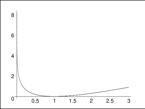
		$\displaystyle I^{d}(u)=\begin{cases}u-1-\log(u),&u>0\\ \infty,&u=0\end{cases}\ \text{(discrete time case)}$
		$\displaystyle I^{c}(u)=\begin{cases}\big(\sqrt{r}-\sqrt{u}\big)^{2},&u>0\\ r,&u=0.\end{cases}\ \text{(continuous time case)}$

Refer to caption — Figure 1. The rate function $I^{d}(u)$

Remark 1.

Related topics to Theorem 2 can be found e.g. in Georgii and Zessin, [3], serving a class of marked point random fields. Probably, the proof of Theorem 2 can be adapted with arguments from proofs in [3] provided that many details not related to our setting have to be omitted and other ones concerning to the boundary effect have to be added.

We prefer to give a complete and direct proof of Theorem 2.

2. Counting random measure, its compensator,
Laplace transform

We consider $(\xi_{i},\tau_{i})_{i\geq 1}$ as a multivariate (marked) point process (see, e.g. [4], [5]) with the counting measure

\mu(dt,dy)=\sum_{i\geq 1}\mathbf{I}_{\{\tau_{i}<\infty\}}\delta_{{\{\tau_{i},\xi_{i}\}}}(t,y)dtdy,

where $\delta_{{\{\tau_{i},\xi_{i}\}}}$ is the Dirac delta-function on $\mathbb{R}_{+}\times\mathbb{R}_{+}$ . Parallel to $(\mathscr{G}_{n})_{n\geq 0}$ , we introduce one more filtration $(\mathscr{G}_{t})_{t\geq 0}$ related to $(\xi_{i},\tau_{i})_{i\geq 1}$ :

\mathscr{G}_{t}:=\sigma(\mu([0,t^{\prime}]\times\varGamma):t^{\prime}\leq t,\varGamma\in\mathscr{B}(\mathbb{R}_{+})),

where $\mathscr{B}(\mathbb{R}_{+})$ is the Borel $\sigma$ -algebra on $\mathbb{R}_{+}$ , and assume that $\mathscr{G}_{0}$ is augmented by $\mathsf{P}$ -zero sets from $\mathcal{F}$ (notice that, then, $(\mathscr{G}_{t})_{t\geq 0}$ satisfies the general conditions). With the help of the counting measure $\mu$ , one can present $tS_{t}$ in a form of a stochastic integral with respect to $\mu$ :

tS_{t}=\int_{0}^{t}\int_{x>0}x\mu(ds,dx).

(2.1)

Then, the Levy measure $\nu(ds,dx)$ , related to $\mu$ , is explicitly computed (see, e.g. Theorem III.1.33, [5])

\nu(ds,dx)=\sum_{i\geq 1}I_{]\hskip-1.5pt]\tau_{i-1},\tau_{i}]\hskip-1.5pt]}(t)\frac{dG(x)de^{-r(s-\tau_{i-1})}}{e^{-r(s-\tau_{i-1})}}=rdsdG(x)

(2.2)

and is not random. It is well known (see, e.g. Corollary to Theorem 1 in §4, Ch.4, [6] that under the deterministic Levy process $tS_{t}$ is the random process with independent increments. We recall a useful property: for any nonnegative and $(\mathscr{G}_{t})$ -predictable function $f(\omega,x,t)$ ,

\mathsf{E}\int_{0}^{t}\int_{x>0}f(\omega,x,s)\mu(ds,dx)=\mathsf{E}\int_{0}^{t}\int_{x>0}f(\omega,x,s)\nu(ds,dx)

with “ $\infty=\infty$ ”.

Lemma 1.

[Laplace transform] For any $\lambda<\Lambda$ and $t>0$ ,

\mathsf{E}e^{\lambda tS_{t}}=e^{rt\int_{x>0}[e^{\lambda z}-1]dG(z)}.

Proof.

Though the direct computation of Laplace’s transform is permissible, we prefer to apply the stochastic calculus. The process $U_{t}=e^{\lambda tS_{t}}$ has right-continuous piece-wise constant paths with jumps

\triangle U_{s}=(U_{s}-U_{s-})=U_{s-}\int_{x>0}[e^{\lambda x}-1]\mu(\{s\},dx),

so that, for any $t>0$ ,

U_{t}=1+\int_{0}^{t}\int_{x>0}U_{s-}[e^{\lambda x}-1]\mu(ds,dx).

Since the function $f(\omega,x,s):=U_{s-}[e^{\lambda x}+1]$ is nonnegative and predictable, the following equality with $\lambda<\Lambda$ holds true:

E\int_{0}^{t}\int_{x>0}U_{s-}[e^{\lambda x}+1]\mu(ds,dx)=E\int_{0}^{t}\int_{x>0}U_{s-}[e^{\lambda x}+1]\nu(ds,dx)\ (<\infty).

Then, we also have

E\int_{0}^{t}\int_{x>0}U_{s-}[e^{\lambda x}-1]\mu(ds,dx)=E\int_{0}^{t}\int_{x>0}U_{s-}[e^{\lambda x}-1]\nu(ds,dx)\ (\in\mathbb{R}).

Since $\nu(ds,dx)=rdsdG(x)$ , the later provides

(\mathsf{E}U_{t})=1+\int_{0}^{t}\int_{x>0}(EU_{s})[e^{\lambda x}-1]dG(x)rds.

This can be written in an equivalent form of differential equation

\frac{d(\mathsf{E}U_{t})}{dt}=(\mathsf{E}U_{t})\int_{x>0}[e^{\lambda x}-1]dG(x)r

subject to $(\mathsf{E}U_{0})=1$ .

Thus, the desired result holds. ∎

3. The proof of Theorem 2

We verify the necessary and sufficient conditions for the LDP to hold (for more details, see Puhalskii, [7]):

1) exponential tightness,

\lim_{j\to\infty}\varlimsup_{t\to\infty}\frac{1}{t}\log\mathsf{P}\big(S_{t}\in\mathbb{R}_{+}\setminus\mathcal{K}_{j}\big)=-\infty,

where $\mathcal{K}_{j}$ ’s are compacts increasing to $\mathbb{R}_{+}$ ;

2) local LDP, defining the rate function $I(u)$ , $u\in\mathbb{R}_{+}$

\lim_{\delta\to 0}\lim_{t\to\infty}\frac{1}{t}\log\mathsf{P}\big(|S_{t}-u|\leq\delta\big).=-I(u).

3.1. The exponential tightness

By choosing

K_{j}=\{x\in\mathbb{R}_{+}:x\in[0,j]\}

and applying Chernoff’s inequality with parameter $0.5\Lambda$ , we find that

\mathsf{P}(S_{t}>j)\leq e^{-0.5\Lambda j+\log\mathsf{E}e^{0.5\Lambda tS_{t}}}.

By Lemma 1,

\mathsf{E}e^{0.5\Lambda tS_{t}}=e^{rt\int_{x>0}[e^{0.5\Lambda x}-1]dG(z)}

and, therefore,

\frac{1}{t}\log\mathsf{P}\big(S_{t}>j\big)\leq-0.5\Lambda j+r\int_{x>0}[e^{0.5\Lambda x}-1]dG(x)\xrightarrow[j\to\infty]{}-\infty

and 1) is done.

3.2. The local LDP

We begin with computation of $I(0)$ and prove

		$\displaystyle\varliminf_{\delta\to 0}\varliminf_{t\to\infty}\frac{1}{t}\log\mathsf{P}(S_{t}\leq\delta)\geq-r[1-G(0+)]$		(3.1)
		$\displaystyle\varlimsup_{\delta\to 0}\varlimsup_{t\to\infty}\frac{1}{t}\log\mathsf{P}(S_{t}\leq\delta)\leq-r[1-G(0+)]$		(3.1)

By (2.2), $\{tS_{t}=0\}=\{\mu((0,t]\times\{x>0\})=0$ . Consequently for any $t>0$ ,

\mathsf{P}(S_{t}\leq\delta)\geq\mathsf{P}(S_{t}=0)=\mathsf{P}(tS_{t}=0)=\mathsf{P}\big(\mu\big((0,t],\{x>0\}\big)=0\big).

The counting process $\pi_{t}:=\mu\big((0,t],\{x>0\}\big)$ has independent increments and the rate

\mathsf{E}\mu\big((0,t],\{x>0\}\big)=\nu\big((0,t],\{x>0\}\big)=r[1-G(0+)]t.

It is a counting process with the compensator $\nu\big((0,t],\{x>0\}\big)=r[1-G(0+)]t.$ Therefore, by the Watanabe theorem, [8], $\pi_{t}$ is a Poisson process with parameter $r[1-G(0+)].$ Hence, due to well known property of the Poisson process

\mathsf{P}(\pi_{t}=0)=e^{-tr[1-G(0+)]}.

We find that

\frac{1}{t}\log\mathsf{P}(S_{t}\leq\delta)\geq\frac{1}{t}\log\mathsf{P}(\pi_{t}=0)=-r[1-G(+)]

implying the lower bond from (3.1).

The upper bound from (3.1) is derived with the help of Laplace’s transform with $0<\lambda<\Lambda$ . To this end, we use identity

1=\mathsf{E}\exp\Big(\lambda tS_{t}-tr\int_{x>0}[e^{\lambda x}-1]dG(x)\Big)

implying the inequality

1\geq\mathsf{E}I_{\{S_{t}\leq\delta\}}\exp\Big(t\Big[\lambda\delta-r\int_{x>0}[e^{\lambda x}-1]dG(x)\Big]\Big)

being equivalent to

\dfrac{1}{t}\log\mathsf{P}(S_{t}\leq\delta)\leq-\lambda\delta+r\int_{x>0}[e^{-\lambda x}-1]dG(x).

Now, passing $t\to\infty$ , we obtain the following upper bound depending on $\delta$ and $\lambda$ :

\varlimsup_{t\to\infty}\frac{1}{t}\log\mathsf{P}(S_{t}\leq\delta)\leq-\lambda\delta+r\int_{x>0}[e^{\lambda x}-1]dG(x).

Now, passing $\delta\to 0$ and $\lambda$ to $-\infty$ we find that

\varlimsup_{\delta\to 0}\varlimsup_{t\to\infty}\frac{1}{t}\log\mathsf{P}(S_{t}\leq\delta)\leq-r\int_{x>0}dG(x)=-r[1-G(0+)].

We continue the proof by checking the formula for $I(u)$ when $u>0$ , i.e.

		$\displaystyle\varlimsup_{\delta\to 0}\varlimsup_{t\to\infty}\frac{1}{t}\log\mathsf{P}(\|S_{t}-u\|\leq\delta)\leq-I(u)$
		$\displaystyle\varliminf_{\delta\to 0}\varliminf_{t\to\infty}\frac{1}{t}\log\mathsf{P}(\|S_{t}-u\|\leq\delta)\geq-I(u),$

with

I(u)=\sup\limits_{\lambda\in(-\infty,\Lambda)}\big[\lambda u-r\int_{0}^{\infty}(e^{\lambda x}-1)dG(x)\big].

The Laplace transform

1=\mathsf{E}\exp\Big(\lambda tS_{t}-tr\int_{x>0}[e^{\lambda x}-1]dG(x)\Big),\ \lambda<\Lambda,

implies the inequality

1\geq\mathsf{E}I_{\{|S_{t}-u|\leq\delta\}}\exp\Big(-t\delta u+\lambda tu-tr\int_{x>0}[e^{\lambda x}-1]dG(x)\Big)

prviding the following upper bound depending on $\lambda$ :

\displaystyle\varlimsup_{\delta\to 0}\varlimsup_{t\to\infty}\frac{1}{t}\log\mathsf{P}(|S_{t}-u|\leq\delta)\leq-\Big(\lambda u-r\int_{x>0}[e^{\lambda x}-1]dG(x)\Big).

A further minimization of the right hand side of the above inequality in $\lambda$ over $(-\infty,\Lambda)$ gives the desired result.

The lower bound proof uses a standard approach of changing “probability measure”. Denote by $\lambda^{*}=\argmax_{\lambda<\Lambda}\big(\lambda u-r\int_{x>0}[e^{\lambda x}-1]dG(x)\big)$ . Since $\lambda^{*}$ solves the equation (with $u>0$ )

u-r\int_{x>0}xe^{\lambda x}dG(x)\big)=0,

(3.2)

$\lambda^{*}$ is a proper number strictly less than $\Lambda$ . Set

\mathfrak{L}_{t}(\lambda^{*})=\exp\Bigg(\lambda^{*}tS_{t}-\int_{0}^{t}\int_{x>0}r[e^{\lambda^{*}x}-1]dG(x)ds\Bigg).

(3.3)

First of all we notice that the Laplace transform for $tS_{t}$ with $\lambda^{*}$ guarantees $\mathsf{E}\mathfrak{L}_{t}(\lambda^{*})=1$ . Moreover, taking into account (2.1) and applying the Itô formula to $\mathfrak{L}_{t}(\lambda^{*})$ one can see that $(\mathfrak{L}_{t}(\lambda^{*}),\mathscr{G}_{t})_{t\geq 0}$ is a positive local martingale with paths from the Skorokhod space $\mathbb{D}_{[0,\infty)}$ . Then a measure $\widetilde{\mathsf{P}}_{t}$ , defined by $d\widetilde{\mathsf{P}}_{t}=\mathfrak{L}_{t}(\lambda^{*})d\mathsf{P}_{t},$ where $\mathsf{P}_{t}$ is a restriction of $\mathsf{P}$ on $\mathscr{G}_{t}$ , is the probability measure. We introduce the probability space $(\varOmega,\mathcal{F},\widetilde{\mathsf{P}}_{t})$ . Since $\mathfrak{L}_{t}(\lambda^{*})>0$ , $\mathsf{P}$ -a.s., not only $\widetilde{\mathsf{P}}_{t}\ll\mathsf{P}_{t}$ but also $\widetilde{\mathsf{P}}_{t}\ll\mathsf{P}_{t}$ with $d\mathsf{P}_{t}=\mathfrak{L}^{-1}_{t}(\lambda^{*})\widetilde{\mathsf{P}}_{t}.$ This property and (3.3) provide a lower bound

	$\displaystyle\mathsf{P}\big(\|S_{t}-u\|\leq\delta\big)$	$\displaystyle=\mathsf{P}_{t}\big(\|S_{t}-u\|\leq\delta\big)=\int_{\{\|S_{t}-u\|\leq\delta\}}\mathfrak{L}^{-1}_{t}(\lambda^{*})d\widetilde{\mathsf{P}}_{t}$
		$\displaystyle\geq e^{-\lambda^{*}t\delta-tI(u)}\widetilde{\mathsf{P}}_{t}\big(\|S_{t}-u\|\leq\delta\big).$

Therefore, we find that

\varliminf_{t\to\infty}\frac{1}{t}\log\mathsf{P}\big(|S_{t}-u|\leq\delta\big)\geq-I(u)-\lambda^{*}\delta+\varliminf_{t\to\infty}\frac{1}{t}\log\widetilde{\mathsf{P}}_{t}\big(|S_{t}-u|\leq\delta\big).

Obviously, the desired lower bound to obtain it is left to prove that

\varliminf_{t\to\infty}\widetilde{\mathsf{P}}_{t}\big(|S_{t}-u|\leq\delta\big)=1

or, equivalently,

\lim_{t\to\infty}\widetilde{\mathsf{P}}_{t}\big(|S_{t}-u|>\delta\big)=0.

(3.4)

Thus the last step of the proof deal with (3.4). To this end, we show that ( $\widetilde{\mathsf{E}}_{t}$ denotes the expectation relative to $\widetilde{\mathsf{P}}_{t}$ )

\lim_{t\to\infty}\widetilde{\mathsf{E}}_{t}|S_{t}-u|^{2}=0.

Since $\mathsf{E}\mathfrak{L}_{t}(\lambda)=1$ , it holds

	$\displaystyle 0=\frac{\partial^{2}\mathsf{E}\mathfrak{L}_{t}(\lambda)}{\partial\lambda^{2}}\|_{\lambda=\lambda^{*}}$
	$\displaystyle=t^{2}\mathsf{E}\Big(S_{t}-r\int_{\{x>0\}}xe^{\lambda^{}x}dG(x)\Big)^{2}\mathfrak{L}_{t}(\lambda^{})-t\underbrace{r\int_{\{x>0\}}x^{2}e^{\lambda^{*}x}dG(x)}_{=u\ \text{(see \eqref{leq})}}$
	$\displaystyle=t^{2}\widetilde{\mathsf{E}}\Big(S_{t}-r\int_{\{x>0\}}xe^{\lambda^{*}x}dG(x)\Big)^{2}-tu.$

Hence,

\widetilde{\mathsf{E}}\big(S_{t}-u\big)^{2}=\frac{1}{t}r\mathsf{E}\int_{\{x>0\}}x^{2}e^{\lambda^{*}x}dG(x)\xrightarrow[t\to\infty]{}0.

∎

References

[1] Cramer, H. (1938) Sur un nouveau theoreme-limite de la theoriedes probabilites. Actualites Santifiques et Industrielles. Colloque cosacrea la throrie des probabilitrs. 3, 736:2–23. Hermann, Paris.
[2] Dembo, A. and Zeitouni, O. (1993) Large Deviations Techniques and Applications. Jones and Bartlet, 1993.
[3] Georgii, Hans-Otto and Zessin, Hans. (1993) Large deviations and the maximum entropy principle of marked point random fields. Probability Theory and Related Fields. 96, 177–204.
[4] Jacod, J. Multivariate point processes: predictable projection, Radon–Nikodym derivatives, representation martingales. Z. Wahrsch. Verw. Gebiete, 31 (1975), 235–53.
[5] Jacod, J. and Shiryaev, A. N. Limit Theorems for Stochastic Processes. Springer-Verlag, New York, Heidelberg, Berlin, (1987).
[6] Liptser, R.S. and Shiryaev, A.N. (1989): Theory of Martingales. Kluwer, Dordrecht (Russian edition 1986)
[7] Puhalskii, A. (2001) Large Deviations and Idempotent Probability, Chapman & Hall/CRC Press.
[8] Watanabe S. (1964) On discontinuous additive functionals and Lévy measures of Markov process. Japan J. Math., 34, 53–70.