跳到论文正文
W Papers独立论文阅读器 arXiv:math/0507167 论文正文 计算阅读时间 · 0%
引用这篇论文根据当前论文元数据生成,正式投稿前建议核对。


License: Assumed arXiv.org perpetual non-exclusive license
arXiv:math/0507167v2 [math.DS] 22 Feb 2007

Algebraic invariants for crystallographic defects in cellular automataMiddletown, CT 06459-0128 USA  * Peterborough, Ontario, Canada, K9L 1Z6.

Marcus Pivato Address: Dept. of Mathematics & Computer Science, Wesleyan University
and Department of Mathematics, Trent University*
Email: marcuspivato@trentu.ca
Abstract

Let 𝒜ℤD{\mathcal{A}}^{{{\mathbb{Z}}^{D}}} be the Cantor space of ℤD{{\mathbb{Z}}^{D}}-indexed configurations in a finite alphabet 𝒜{\mathcal{A}}, and let σ\sigma be the ℤD{{\mathbb{Z}}^{D}}-action of shifts on 𝒜ℤD{\mathcal{A}}^{{{\mathbb{Z}}^{D}}}. A cellular automaton is a continuous, σ\sigma-commuting self-map Φ\Phi of 𝒜ℤD{\mathcal{A}}^{{{\mathbb{Z}}^{D}}}, and a Φ\Phi-invariant subshift is a closed, (Φ,σ)(\Phi,\sigma)-invariant subset 𝔄⊂𝒜ℤD{\mathfrak{A}}\subset{\mathcal{A}}^{{{\mathbb{Z}}^{D}}}. Suppose 𝐚∈𝒜ℤD{\mathbf{a}}\in{\mathcal{A}}^{{{\mathbb{Z}}^{D}}} is 𝔄{\mathfrak{A}}-admissible everywhere except for some small region we call a defect. It has been empirically observed that such defects persist under iteration of Φ\Phi, and often propagate like ‘particles’ which coalesce or annihilate on contact. We construct algebraic invariants for these defects, which explain their persistence under Φ\Phi, and partly explain the outcomes of their collisions. Some invariants are based on the cocycles of multidimensional subshifts; others arise from the higher-dimensional (co)homology/homotopy groups for subshifts, obtained by generalizing the Conway-Lagarias tiling groups and the Geller-Propp fundamental group.

MSC: 37B50 (primary), 37B15, 37A20 (secondary)
Keywords: Cellular automata, subshift, cocycle, cohomology, tiling group,
defect, kink, domain boundary.
\ETDS

19924027(#1)2007 \runningheadsM. PivatoAlgebraic invariants for crystallographic defects in cellular automata

\recd

10 August 2005 and accepted 29 June 2006

A striking phenomenon in cellular automata is the emergence of homogeneous ‘domains’ (each exhibiting a particular spatial pattern), punctuated by defects (analogous to ‘domain boundaries’ or ‘kinks’ in a crystalline solid) which evolve and propagate over time, and occasionally collide. This phenomenon has been studied empirically in [Gra84b, Gra84a, KS88, BR91, BNR91, Han93, CH92, CH93a, CH93b, CH97, CHM98] and theoretically in [Lin84, EN92, Elo93a, Elo93b, Elo94, CHS01, KM00, K ̵̊ur03, KM02, K ̵̊ur03, K ̵̊ur05]; see [Piv07a, Piv07b] for a summary. The mathematical theory of cellular automaton defect dynamics is still in its infancy. Even the term ‘defect’ does not yet have a unanimous definition. Other open questions include:

  1. 1.

    Why do defects persist under the action of cellular automata, rather than disappearing? Are there ‘topological’ constraints imposed by the structure of the underlying domain, which make defects indestructible?

  2. 2.

    When defects collide, they often coalesce into a new type of defect, or mutually annihilate. Is there a ‘chemistry’ governing these defect collisions?

  3. 3.

    Can we assign algebraic invariants to defects, which reflect (a) the ‘topological constraints’ of question #1 or (b) the ‘defect chemistry’ of question #2?

In a companion paper [Piv07b], we developed a new framework for describing defects, and used spectral theory to get invariants (as in question #3) for codimension-one (‘domain boundary’) defects. Unfortunately, these spectral invariants were not applicable to defects of codimension two or higher (e.g. ‘holes’ in ℤ2{\mathbb{Z}}^{2}, ‘strings’ in ℤ3{\mathbb{Z}}^{3}, etc.). In this paper, we will answer question #3 for such defects, using methods inspired by algebraic topology.

This paper is organized as follows: in §1 we review the framework developed in [Piv07b]. We also define defect codimension, and introduce many examples which recur throughout the paper. In §2, we address question #3 using dynamical cohomology, while in §3, we address #3 using tiling homotopy/(co)homology groups. In §4 we relate the dynamical cohomology of §2 to the tiling cohomology of §3. In all cases, we are able to use these algebraic invariants to answer question #1, and partially answer question #2.

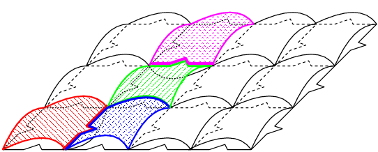
The diagram at right portrays the logical dependency of these sections. In particular, notice that §2 and §3 are logically independent of one another, although §4 depends upon both. Our main results are in sections 2.2, 2.3, 3.5, and 4.2.    [Uncaptioned image]

Preliminaries & Notation:

Let 𝒜{\mathcal{A}} be a finite alphabet. Let D≥1D\geq 1, let ℤD{{\mathbb{Z}}^{D}} be the DD-dimensional lattice, and let 𝒜ℤD{\mathcal{A}}^{{{\mathbb{Z}}^{D}}} be the set of all ℤD{{\mathbb{Z}}^{D}}-indexed configurations of the form 𝐚=[a𝗓]𝗓∈ℤD{\mathbf{a}}=[a_{{\mathsf{z}}}]_{{\mathsf{z}}\in{{\mathbb{Z}}^{D}}}, where a𝗓∈𝒜a_{\mathsf{z}}\in{\mathcal{A}} for all 𝗓∈ℤD{\mathsf{z}}\in{{\mathbb{Z}}^{D}}. The Cantor metric on 𝒜ℤD{\mathcal{A}}^{{{\mathbb{Z}}^{D}}} is defined by d⁡(𝐚,𝐛)=2−Δ⁡(𝐚,𝐛)d({\mathbf{a}},{\mathbf{b}})=2^{-\Delta({\mathbf{a}},{\mathbf{b}})}, where Δ⁡(𝐚,𝐛):=min⁡{|𝗓|;a𝗓≠b𝗓}\Delta({\mathbf{a}},{\mathbf{b}}):=\min{\left\{|{\mathsf{z}}|\;;\;a_{\mathsf{z}}\neq b_{\mathsf{z}}\right\}}. It follows that (𝒜ℤD,d)({\mathcal{A}}^{{{\mathbb{Z}}^{D}}},d) is a Cantor space (i.e. a compact, totally disconnected, perfect metric space). If 𝐚∈𝒜ℤD{\mathbf{a}}\in{\mathcal{A}}^{{{\mathbb{Z}}^{D}}} and 𝕌⊂ℤD{\mathbb{U}}\subset{{\mathbb{Z}}^{D}}, then we define 𝐚𝕌∈𝒜𝕌{\mathbf{a}}_{\mathbb{U}}\in{\mathcal{A}}^{\mathbb{U}} by 𝐚𝕌:=[a𝗎]𝗎∈𝕌{\mathbf{a}}_{\mathbb{U}}:=[a_{\mathsf{u}}]_{{\mathsf{u}}\in{\mathbb{U}}}. If 𝗓∈ℤD{\mathsf{z}}\in{{\mathbb{Z}}^{D}}, then strictly speaking, 𝐚𝗓+𝕌∈𝒜𝗓+𝕌{\mathbf{a}}_{{\mathsf{z}}+{\mathbb{U}}}\in{\mathcal{A}}^{{\mathsf{z}}+{\mathbb{U}}}; however, it will often be convenient to ‘abuse notation’ and treat 𝐚𝗓+𝕌{\mathbf{a}}_{{\mathsf{z}}+{\mathbb{U}}} as an element of 𝒜𝕌{\mathcal{A}}^{{\mathbb{U}}} in the obvious way.

For any 𝗏∈ℤD{\mathsf{v}}\in{{\mathbb{Z}}^{D}}, we define the shift σ𝗏:𝒜ℤD⟶𝒜ℤD\sigma^{{\mathsf{v}}}:{\mathcal{A}}^{{{\mathbb{Z}}^{D}}}{{\longrightarrow}}{\mathcal{A}}^{{{\mathbb{Z}}^{D}}} by σ𝗏​(𝐚)𝗓=a𝗓+𝗏\sigma^{{\mathsf{v}}}({\mathbf{a}})_{{\mathsf{z}}}=a_{{\mathsf{z}}+{\mathsf{v}}} for all 𝐚∈𝒜ℤD{\mathbf{a}}\in{\mathcal{A}}^{{{\mathbb{Z}}^{D}}} and 𝗓∈ℤD{\mathsf{z}}\in{{\mathbb{Z}}^{D}}. A cellular automaton is a transformation Φ:𝒜ℤD⟶𝒜ℤD\Phi:{\mathcal{A}}^{{{\mathbb{Z}}^{D}}}{{\longrightarrow}}{\mathcal{A}}^{{{\mathbb{Z}}^{D}}} that is continuous and commutes with all shifts. Equivalently, Φ\Phi is determined by a local rule ϕ:𝒜ℍ⟶𝒜\phi:{\mathcal{A}}^{\mathbb{H}}{{\longrightarrow}}{\mathcal{A}} such that Φ​(𝐚)𝗓=ϕ⁡(𝐚𝗓+ℍ)\Phi({\mathbf{a}})_{{\mathsf{z}}}=\phi({\mathbf{a}}_{{\mathsf{z}}+{\mathbb{H}}}) for all 𝐚∈𝒜ℤD{\mathbf{a}}\in{\mathcal{A}}^{{{\mathbb{Z}}^{D}}} and 𝗓∈ℤD{\mathsf{z}}\in{{\mathbb{Z}}^{D}} [Hed69]. Here, ℍ⊂ℤD{\mathbb{H}}\subset{{\mathbb{Z}}^{D}} is a finite set which we normally imagine as a ‘neighbourhood of the origin’. If ℍ⊆𝔹⁡(r):=[−r​…​r]D{\mathbb{H}}\subseteq{\mathbb{B}}(r):={\left[-r...r\right]}^{D}, we say that Φ\Phi has radius rr.

A subset 𝔄⊂𝒜ℤD{\mathfrak{A}}\subset{\mathcal{A}}^{{{\mathbb{Z}}^{D}}} is a subshift [LM95, Kit98] if 𝔄{\mathfrak{A}} is closed in the Cantor topology, and if σ𝗓​(𝔄)=𝔄\sigma^{{\mathsf{z}}}({\mathfrak{A}})={\mathfrak{A}} for all 𝗓∈ℤD{\mathsf{z}}\in{{\mathbb{Z}}^{D}}. For any 𝕌⊂ℤD{\mathbb{U}}\subset{{\mathbb{Z}}^{D}}, we define 𝔄𝕌:={𝐚𝕌;𝐚∈𝔄}{\mathfrak{A}}_{\mathbb{U}}:={\left\{{\mathbf{a}}_{\mathbb{U}}\;;\;{\mathbf{a}}\in{\mathfrak{A}}\right\}}. In particular, for any r>0r>0, let 𝔄(r):=𝔄𝔹⁡(r){\mathfrak{A}}_{(r)}:={\mathfrak{A}}_{{\mathbb{B}}(r)} be the set of admissible rr-blocks for 𝔄{\mathfrak{A}}. We say 𝔄{\mathfrak{A}} is a subshift of finite type (SFT) if there is some r>0r>0 (the radius of 𝔄{\mathfrak{A}}) such that 𝔄{\mathfrak{A}} is entirely described by 𝔄(r){\mathfrak{A}}_{(r)}, in the sense that 𝔄={𝐚∈𝒜ℤD;𝐚𝔹⁡(𝗓,r)∈𝔄(r),∀𝗓∈ℤD}{\mathfrak{A}}={\left\{{\mathbf{a}}\in{\mathcal{A}}^{{{\mathbb{Z}}^{D}}}\;;\;{\mathbf{a}}_{{\mathbb{B}}({\mathsf{z}},r)}\in{\mathfrak{A}}_{(r)},\ \forall{\mathsf{z}}\in{{\mathbb{Z}}^{D}}\right\}}. If D=1D=1, then a Markov subshift is an SFT 𝔄⊂𝒜ℤ{\mathfrak{A}}\subset{\mathcal{A}}^{\mathbb{Z}} determined by a set 𝔄{0,1}⊂𝒜{0,1}{\mathfrak{A}}_{\{0,1\}}\subset{\mathcal{A}}^{\{0,1\}} of admissible transitions; equivalently, 𝔄{\mathfrak{A}} is the set of all bi-infinite directed paths in a digraph whose vertices are the elements of 𝔄{\mathfrak{A}}, with an edge a↝ba\leadsto b iff (a,b)∈𝔄{0,1}(a,b)\in{\mathfrak{A}}_{\{0,1\}}. If D=2D=2, then let 𝔼1:={(0,0),(1,0)}{\mathbb{E}}_{1}:=\{(0,0),(1,0)\} and 𝔼2:={(0,0),(0,1)}{\mathbb{E}}_{2}:=\{(0,0),(0,1)\}. A Wang subshift is an SFT 𝔄⊂𝒜ℤ2{\mathfrak{A}}\subset{\mathcal{A}}^{{{\mathbb{Z}}^{2}}} determined by sets 𝔄𝔼1⊂𝒜𝔼1{\mathfrak{A}}_{{\mathbb{E}}_{1}}\subset{\mathcal{A}}^{{\mathbb{E}}_{1}} and 𝔄𝔼2⊂𝒜𝔼2{\mathfrak{A}}_{{\mathbb{E}}_{2}}\subset{\mathcal{A}}^{{\mathbb{E}}_{2}} of edge-matching conditions. Equivalently, 𝔄{\mathfrak{A}} is the set of all tilings of the plane ℝ2{{\mathbb{R}}^{2}} by unit square tiles (corresponding to the elements of 𝒜{\mathcal{A}}) with notched edges representing the edge-matching conditions [GS87, Ch.11]. More generally, if D≥3D\geq 3, then for all d∈[1​…​D]d\in{\left[1...D\right]}, let 𝔼d:={0}d−1×{0,1}×{0}D−d{\mathbb{E}}_{d}:=\{0\}^{d-1}\times\{0,1\}\times\{0\}^{D-d}. A Wang subshift is an SFT 𝔄⊂𝒜ℤD{\mathfrak{A}}\subset{\mathcal{A}}^{{{\mathbb{Z}}^{D}}} determined by sets 𝔄𝔼d⊂𝒜𝔼d{\mathfrak{A}}_{{\mathbb{E}}_{d}}\subset{\mathcal{A}}^{{\mathbb{E}}_{d}} of face-matching conditions for d∈[1​…​D]d\in{\left[1...D\right]}. Equivalently, 𝔄{\mathfrak{A}} is the set of tesselations of ℝD{{\mathbb{R}}^{D}} by unit (hyper)cubes with ‘notched’ faces.

If 𝒳{\mathcal{X}} is any set and F:𝔄⟶𝒳F:{\mathfrak{A}}{{\longrightarrow}}{\mathcal{X}} is a function, then FF is locally determined if there is some radius r∈ℕr\in{\mathbb{N}} and some local rule f:𝔄(r)⟶𝒳f:{\mathfrak{A}}_{(r)}{{\longrightarrow}}{\mathcal{X}} such that F⁡(𝐚)=f⁡(𝐚𝔹⁡(r))F({\mathbf{a}})=f({\mathbf{a}}_{{\mathbb{B}}(r)}) for any 𝐚∈𝔄{\mathbf{a}}\in{\mathfrak{A}}. If 𝒳{\mathcal{X}} is any discrete space, then F:𝔄⟶𝒳F:{\mathfrak{A}}{{\longrightarrow}}{\mathcal{X}} is continuous iff FF is locally determined. For example, if 𝒜{\mathcal{A}} and ℬ{\mathcal{B}} are finite sets, then a (subshift) homomorphism is a continuous, σ\sigma-commuting function Φ:ℬℤD⟶𝒜ℤD\Phi:{\mathcal{B}}^{{{\mathbb{Z}}^{D}}}{{\longrightarrow}}{\mathcal{A}}^{{{\mathbb{Z}}^{D}}} (e.g. a CA is a homomorphism with 𝒜=ℬ{\mathcal{A}}={\mathcal{B}}); it follows that F⁡(𝐚)=Φ​(𝐚)0F({\mathbf{a}})=\Phi({\mathbf{a}})_{0} is locally determined. If 𝔅⊂ℬℤD{\mathfrak{B}}\subset{\mathcal{B}}^{{{\mathbb{Z}}^{D}}} is a subshift of finite type, and Ψ:ℬℤD⟶𝒜ℤD\Psi:{\mathcal{B}}^{{{\mathbb{Z}}^{D}}}{{\longrightarrow}}{\mathcal{A}}^{{{\mathbb{Z}}^{D}}} is a homomorphism, then 𝔄:=Ψ⁡(𝔅)⊂𝒜ℤD{\mathfrak{A}}:=\Psi({\mathfrak{B}})\subset{\mathcal{A}}^{{{\mathbb{Z}}^{D}}} is called a sofic shift.

If Φ:𝒜ℤD⟶𝒜ℤD\Phi:{\mathcal{A}}^{{{\mathbb{Z}}^{D}}}{{\longrightarrow}}{\mathcal{A}}^{{{\mathbb{Z}}^{D}}} is a cellular automaton, then we say 𝔄{\mathfrak{A}} is (weakly) Φ\Phi-invariant if Φ⁡(𝔄)⊆𝔄\Phi({\mathfrak{A}})\subseteq{\mathfrak{A}} (i.e. Φ\Phi is an endomorphism of 𝔄{\mathfrak{A}}). For example, if p∈ℕp\in{\mathbb{N}} and 𝗏∈ℤD{\mathsf{v}}\in{{\mathbb{Z}}^{D}}, then the set 𝖥𝗂𝗑⁡[Φp]{\sf Fix}\left[\Phi^{p}\right] of (Φ,p)(\Phi,p)-periodic points and the set 𝖥𝗂𝗑⁡[Φp∘σ−p​𝗏]{\sf Fix}\left[\Phi^{p}\circ\sigma^{-p{\mathsf{v}}}\right] of (Φ,p,𝗏)(\Phi,p,{\mathsf{v}})-travelling waves are Φ\Phi-invariant SFTs. If Φ∞​(𝒜ℤD):=⋂t=1∞Φt​(𝒜ℤD)\Phi^{\infty}({\mathcal{A}}^{{{\mathbb{Z}}^{D}}}):=\bigcap_{t=1}^{\infty}\Phi^{t}({\mathcal{A}}^{{{\mathbb{Z}}^{D}}}) is the eventual image of Φ\Phi, then Φ∞​(𝒜ℤD)\Phi^{\infty}({\mathcal{A}}^{{{\mathbb{Z}}^{D}}}) is a Φ\Phi-invariant subshift (possibly non-sofic), which contains 𝖥𝗂𝗑⁡[Φp∘σ−p​𝗏]{\sf Fix}\left[\Phi^{p}\circ\sigma^{-p{\mathsf{v}}}\right] for any p∈ℕp\in{\mathbb{N}} and 𝗏∈ℤD{\mathsf{v}}\in{{\mathbb{Z}}^{D}}.

If 𝗒,𝗓∈ℤD{\mathsf{y}},{\mathsf{z}}\in{{\mathbb{Z}}^{D}}, then we write “𝗒↝𝗓{\mathsf{y}}\stackrel{{\scriptstyle}}{{\leadsto}}{\mathsf{z}}” if |𝗓−𝗒|=1|{\mathsf{z}}-{\mathsf{y}}|=1. A trail is a sequence ζ=(𝗓1↝𝗓2↝⋯↝𝗓n)\zeta=({\mathsf{z}}_{1}\stackrel{{\scriptstyle}}{{\leadsto}}{\mathsf{z}}_{2}\stackrel{{\scriptstyle}}{{\leadsto}}\cdots\stackrel{{\scriptstyle}}{{\leadsto}}{\mathsf{z}}_{n}). A subset 𝕐⊂ℤD{\mathbb{Y}}\subset{{\mathbb{Z}}^{D}} is trail-connected if, for any 𝗑,𝗒∈𝕐{\mathsf{x}},{\mathsf{y}}\in{\mathbb{Y}}, there is a trail 𝗑=𝗓0↝𝗓1↝⋯↝𝗓n=𝗒{\mathsf{x}}={\mathsf{z}}_{0}\stackrel{{\scriptstyle}}{{\leadsto}}{\mathsf{z}}_{1}\stackrel{{\scriptstyle}}{{\leadsto}}\cdots\stackrel{{\scriptstyle}}{{\leadsto}}{\mathsf{z}}_{n}={\mathsf{y}} in 𝕐{\mathbb{Y}}.

Font conventions:

Upper case calligraphic letters (𝒜,ℬ,𝒞,…{\mathcal{A}},{\mathcal{B}},{\mathcal{C}},\ldots) denote alphabets or groups. Upper-case Gothic letters (𝔄,𝔅,ℭ,…{\mathfrak{A}},{\mathfrak{B}},{\mathfrak{C}},\ldots) denote subsets of 𝒜ℤD{\mathcal{A}}^{{{\mathbb{Z}}^{D}}} (e.g. subshifts), lowercase bold-faced letters (𝐚,𝐛,𝐜,…{\mathbf{a}},{\mathbf{b}},{\mathbf{c}},\ldots) denote elements of 𝒜ℤD{\mathcal{A}}^{{{\mathbb{Z}}^{D}}}, and Roman letters (a,b,c,…a,b,c,\ldots) are elements of 𝒜{\mathcal{A}} or ordinary numbers. Lower-case sans-serif (…,𝗑,𝗒,𝗓\ldots,{\mathsf{x}},{\mathsf{y}},{\mathsf{z}}) are elements of ℤD{{\mathbb{Z}}^{D}}, upper-case hollow font (𝕌,𝕍,𝕎,…{\mathbb{U}},{\mathbb{V}},{\mathbb{W}},\ldots) are subsets of ℤD{{\mathbb{Z}}^{D}}, and upper-case bold (𝐔,𝐕,𝐖,…{\mathbf{U}},{\mathbf{V}},{\mathbf{W}},\ldots) are subsets of ℝD{{\mathbb{R}}^{D}}. Upper-case Greek letters (Φ,Ψ,…\Phi,\Psi,\ldots) are functions on 𝒜ℤD{\mathcal{A}}^{{{\mathbb{Z}}^{D}}} (e.g. CA), and lower-case Greek letters (ϕ,ψ,…\phi,\psi,\ldots) are other functions (e.g. local rules.)

1 Defects and Codimension

Let 𝔄⊂𝒜ℤD{\mathfrak{A}}\subset{\mathcal{A}}^{{{\mathbb{Z}}^{D}}} be any subshift. If 𝐚∈𝒜ℤD{\mathbf{a}}\in{\mathcal{A}}^{{{\mathbb{Z}}^{D}}}, then the defect field ℱ𝐚:ℤD⟶ℕ∪{∞}{\mathcal{F}}_{{\mathbf{a}}}:{{\mathbb{Z}}^{D}}{{\longrightarrow}}{\mathbb{N}}\cup\{{\infty}\} is defined by ℱ𝐚​(𝗓):=max⁡{r∈ℕ;𝐚𝔹⁡(𝗓,r)∈𝔄(r)}{\mathcal{F}}_{{\mathbf{a}}}({\mathsf{z}})\ :=\ \max{\left\{r\in{\mathbb{N}}\;;\;{\mathbf{a}}_{{\mathbb{B}}({\mathsf{z}},r)}\in{\mathfrak{A}}_{(r)}\right\}}, for all 𝗓∈ℤD{\mathsf{z}}\in{{\mathbb{Z}}^{D}}. Clearly, ℱ𝐚{\mathcal{F}}_{{\mathbf{a}}} is ‘Lipschitz’ in the sense that |ℱ𝐚​(𝗒)−ℱ𝐚​(𝗓)|≤|𝗒−𝗓||{\mathcal{F}}_{{\mathbf{a}}}({\mathsf{y}})-{\mathcal{F}}_{{\mathbf{a}}}({\mathsf{z}})|\leq|{\mathsf{y}}-{\mathsf{z}}|. The defect set of 𝐚{\mathbf{a}} is the set 𝔻⁡(𝐚)⊂ℤD{\mathbb{D}}({\mathbf{a}})\subset{{\mathbb{Z}}^{D}} of local minima of ℱ𝐚{\mathcal{F}}_{{\mathbf{a}}}. See [Piv07b, §1] for further discussion.

  • Example 1.1: (a) Suppose 𝔄{\mathfrak{A}} is an SFT determined by a set 𝔄(r)⊂𝒜𝔹⁡(r){\mathfrak{A}}_{(r)}\subset{\mathcal{A}}^{{\mathbb{B}}(r)} of admissible rr-blocks, and let 𝕏:={𝗓∈ℤD;𝐚𝔹⁡(𝗓,r)∉𝔄(r)}{\mathbb{X}}:={\left\{{\mathsf{z}}\in{{\mathbb{Z}}^{D}}\;;\;{\mathbf{a}}_{{\mathbb{B}}({\mathsf{z}},r)}\not\in{\mathfrak{A}}_{(r)}\right\}}. Assume for simplicity that 𝔄(r−1)=𝒜𝔹⁡(r−1){\mathfrak{A}}_{(r-1)}={\mathcal{A}}^{{\mathbb{B}}(r-1)}. Then ℱ𝐚​(𝗓)=r+d⁡(𝗓,𝕏){\mathcal{F}}_{{\mathbf{a}}}({\mathsf{z}})=r+d({\mathsf{z}},{\mathbb{X}}), where d⁡(𝗓,𝕏):=min𝗑∈𝕏⁡|𝗓−𝗑|d({\mathsf{z}},{\mathbb{X}}):=\displaystyle\min_{{\mathsf{x}}\in{\mathbb{X}}}\ |{\mathsf{z}}-{\mathsf{x}}|. In particular, ℱ𝐚​(𝗓)=r{\mathcal{F}}_{{\mathbf{a}}}({\mathsf{z}})=r if and only if 𝗓∈𝕏{\mathsf{z}}\in{\mathbb{X}}, and this is the smallest possible value for ℱ𝐚​(𝗓){\mathcal{F}}_{{\mathbf{a}}}({\mathsf{z}}). Thus, 𝔻⁡(𝐚)=𝕏{\mathbb{D}}({\mathbf{a}})={\mathbb{X}}.

    (b) Let 𝒜=ℬ∪𝒟{\mathcal{A}}={\mathcal{B}}\cup{\mathcal{D}} and let 𝔄:=ℬℤD∪𝒟ℤD{\mathfrak{A}}:={\mathcal{B}}^{{{\mathbb{Z}}^{D}}}\cup{\mathcal{D}}^{{{\mathbb{Z}}^{D}}}. Let 𝒞:=ℬ∩𝒟{\mathcal{C}}:={\mathcal{B}}\cap{\mathcal{D}}, and let ℬ∗:=ℬ∖𝒞{\mathcal{B}}^{*}:={\mathcal{B}}\setminus{\mathcal{C}} and 𝒟∗:=𝒟∖𝒞{\mathcal{D}}^{*}:={\mathcal{D}}\setminus{\mathcal{C}}. Any 𝐚∈𝒜ℤD{\mathbf{a}}\in{\mathcal{A}}^{{{\mathbb{Z}}^{D}}} is a mixture of ℬ∗{\mathcal{B}}^{*}-symbols, 𝒞{\mathcal{C}}-symbols, and 𝒟∗{\mathcal{D}}^{*}-symbols. If 𝗓∈ℤD{\mathsf{z}}\in{{\mathbb{Z}}^{D}} and a𝗓∈ℬ∗a_{\mathsf{z}}\in{\mathcal{B}}^{*}, then ℱ𝐚​(𝗓)=min⁡{|𝗒−𝗓|;a𝗒∈𝒟∗}{\mathcal{F}}_{{\mathbf{a}}}({\mathsf{z}})=\min{\left\{|{\mathsf{y}}-{\mathsf{z}}|\;;\;a_{\mathsf{y}}\in{\mathcal{D}}^{*}\right\}}. If a𝗓∈𝒟∗a_{\mathsf{z}}\in{\mathcal{D}}^{*}, then ℱ𝐚​(𝗓)=min⁡{|𝗒−𝗓|;a𝗒∈ℬ∗}{\mathcal{F}}_{{\mathbf{a}}}({\mathsf{z}})=\min{\left\{|{\mathsf{y}}-{\mathsf{z}}|\;;\;a_{\mathsf{y}}\in{\mathcal{B}}^{*}\right\}}. If a𝗓∈𝒞a_{\mathsf{z}}\in{\mathcal{C}}, then ℱ𝐚(𝗓)=min{r;a𝗑∈ℬ∗ and a𝗒∈ℬ∗{\mathcal{F}}_{{\mathbf{a}}}({\mathsf{z}})=\min\{r\ ;\ a_{\mathsf{x}}\in{\mathcal{B}}^{*}\mbox{\ and \ }a_{\mathsf{y}}\in{\mathcal{B}}^{*} for some 𝗑,𝗒∈𝔹⁡(𝗓,r)}\ \mbox{for some ${\mathsf{x}},{\mathsf{y}}\in{\mathbb{B}}({\mathsf{z}},r)$}\}. Thus, 𝔻⁡(𝐚){\mathbb{D}}({\mathbf{a}}) is the set of all points which are either on a ‘boundary’ between a ℬ∗{\mathcal{B}}^{*}-domain and a 𝒟∗{\mathcal{D}}^{*}-domain, or roughly in the middle of a 𝒞{\mathcal{C}}-domain. ♢\diamondsuit

Let 𝔄~:={𝐚∈𝒜ℤD;sup𝗓∈ℤDℱ𝐚(𝗓)=∞}\widetilde{{\mathfrak{A}}}:={\left\{{\mathbf{a}}\in{\mathcal{A}}^{{{\mathbb{Z}}^{D}}}\;;\;\displaystyle\sup_{{\mathsf{z}}\in{{\mathbb{Z}}^{D}}}\ {\mathcal{F}}_{{\mathbf{a}}}({\mathsf{z}})\ =\ {\infty}\right\}} be the set of ‘slightly defective’ configurations. If 𝐚∈𝔄~∖𝔄{\mathbf{a}}\in\widetilde{{\mathfrak{A}}}\setminus{\mathfrak{A}}, then we say 𝐚{\mathbf{a}} is defective. Elements of 𝔄~\widetilde{{\mathfrak{A}}} may have infinitely large defects, but also have arbitrarily large non-defective regions. Clearly 𝔄⊂𝔄~{\mathfrak{A}}\subset\widetilde{{\mathfrak{A}}}, and 𝔄~\widetilde{{\mathfrak{A}}} is a σ\sigma-invariant, dense subset of 𝒜ℤD{\mathcal{A}}^{{{\mathbb{Z}}^{D}}} (but not a subshift).

For any R>0R>0, let 𝔾R​(𝐚):={𝗓∈ℤD;ℱ𝐚​(𝗓)≥R}{\mathbb{G}}_{R}({\mathbf{a}}):={\left\{{\mathsf{z}}\in{{\mathbb{Z}}^{D}}\;;\;{\mathcal{F}}_{{\mathbf{a}}}({\mathsf{z}})\geq R\right\}}. Thus, 𝐚∈𝔄~{\mathbf{a}}\in\widetilde{{\mathfrak{A}}} iff 𝔾R​(𝐚)≠∅{\mathbb{G}}_{R}({\mathbf{a}})\neq\emptyset for all R>0R>0. For example, if 𝔄{\mathfrak{A}} is an SFT determined by a set 𝔄(r){\mathfrak{A}}_{(r)} of admissible rr-blocks, and 𝔻={𝗓∈ℤD;𝐚𝔹⁡(𝗓,r)∉𝔄(r)}{\mathbb{D}}={\left\{{\mathsf{z}}\in{{\mathbb{Z}}^{D}}\;;\;{\mathbf{a}}_{{\mathbb{B}}({\mathsf{z}},r)}\not\in{\mathfrak{A}}_{(r)}\right\}} as in Example 1(a), then 𝔾R​(𝐚)={𝗓∈ℤD;d⁡(𝗓,𝔻)≥R−r}=ℤD∖𝔹⁡(𝔻,R−r){\mathbb{G}}_{R}({\mathbf{a}})={\left\{{\mathsf{z}}\in{{\mathbb{Z}}^{D}}\;;\;d({\mathsf{z}},{\mathbb{D}})\geq R-r\right\}}={{\mathbb{Z}}^{D}}\setminus{\mathbb{B}}({\mathbb{D}},R-r). Thus, 𝔻⁡(𝐚){\mathbb{D}}({\mathbf{a}}) encodes all information about the ‘defect structure’ of 𝐚{\mathbf{a}}. However, if 𝔄{\mathfrak{A}} is not an SFT [e.g. Example 1(b)], then in general 𝔾R​(𝐚)≠ℤD∖𝔹⁡(𝔻,R′){\mathbb{G}}_{R}({\mathbf{a}})\neq{{\mathbb{Z}}^{D}}\setminus{\mathbb{B}}({\mathbb{D}},R^{\prime}) for any R′>0R^{\prime}>0. In this case, 𝔻⁡(𝐚){\mathbb{D}}({\mathbf{a}}) is an inadequate description of the larger-scale ‘defect structures’ of 𝐚{\mathbf{a}}. Thus, instead of treating the defect as a precisely defined subset of ℤD{{\mathbb{Z}}^{D}}, it is better to think of it as a ‘fuzzy’ object residing in the low areas in the defect field ℱ𝐚{\mathcal{F}}_{{\mathbf{a}}}. The advantage of this approach is its applicability to any kind of subshift (finite type, sofic, or otherwise). Nevertheless, most of our examples will be SFTs, and we may then refer to the specific region 𝔻⊂ℤD{\mathbb{D}}\subset{{\mathbb{Z}}^{D}} as ‘the defect’.

Proposition 1.2

Let Φ:𝒜ℤD⟶𝒜ℤD\Phi:{\mathcal{A}}^{{{\mathbb{Z}}^{D}}}{{\longrightarrow}}{\mathcal{A}}^{{{\mathbb{Z}}^{D}}} be a CA with radius r>0r>0.

  • (a)

    Let 𝔄⊂𝒜ℤD{\mathfrak{A}}\subset{\mathcal{A}}^{{{\mathbb{Z}}^{D}}} be a weakly Φ\Phi-invariant subshift. Then Φ⁡(𝔄~)⊆𝔄~\Phi(\widetilde{{\mathfrak{A}}})\subseteq\widetilde{{\mathfrak{A}}}.

  • (b)

    If 𝐚∈𝔄~{\mathbf{a}}\in\widetilde{{\mathfrak{A}}}, and 𝐚′=Φ⁡(𝐚){\mathbf{a}}^{\prime}=\Phi({\mathbf{a}}), then ℱ𝐚′≥ℱ𝐚−r{\mathcal{F}}_{{\mathbf{a}}^{\prime}}\geq{\mathcal{F}}_{{\mathbf{a}}}-r. Thus, for all R∈ℕR\in{\mathbb{N}}, 𝔾R+r​(𝐚)⊆𝔾R​(𝐚′){\mathbb{G}}_{R+r}({\mathbf{a}})\subseteq{\mathbb{G}}_{R}({\mathbf{a}}^{\prime}).

  • Proof: (b) Let 𝗓∈ℤD{\mathsf{z}}\in{{\mathbb{Z}}^{D}} and suppose ℱ𝐚​(𝗓)=R{\mathcal{F}}_{{\mathbf{a}}}({\mathsf{z}})=R. Thus, 𝐚𝔹⁡(𝗓,R)∈𝔄R{\mathbf{a}}_{{\mathbb{B}}({\mathsf{z}},R)}\in{\mathfrak{A}}_{R}. But 𝔄{\mathfrak{A}} is Φ\Phi-invariant; hence 𝐚𝔹⁡(𝗓,R−r)′∈𝔄(R−r){\mathbf{a}}^{\prime}_{{\mathbb{B}}({\mathsf{z}},R-r)}\in{\mathfrak{A}}_{(R-r)}. Hence ℱ𝐚′​(𝗓)≥R−r{\mathcal{F}}_{{\mathbf{a}}^{\prime}}({\mathsf{z}})\geq R-r. Then (a) follows from (b). □\Box

Let Φ:𝒜ℤD⟶𝒜ℤD\Phi:{\mathcal{A}}^{{{\mathbb{Z}}^{D}}}{{\longrightarrow}}{\mathcal{A}}^{{{\mathbb{Z}}^{D}}} be a cellular automaton, and suppose that ϕ⁡(𝔄)=𝔄\phi({\mathfrak{A}})={\mathfrak{A}}. If 𝐚∈𝔄~{\mathbf{a}}\in\widetilde{{\mathfrak{A}}} then 𝐚{\mathbf{a}} has a Φ\Phi-persistent defect if, for all t∈ℕt\in{\mathbb{N}}, 𝐚′=Φt​(𝐚){\mathbf{a}}^{\prime}=\Phi^{t}({\mathbf{a}}) is also defective. Otherwise 𝐚{\mathbf{a}} has a transient defect —i.e. one which eventually disappears. We say 𝐚{\mathbf{a}} has a removable defect if there is some r>0r>0 and some 𝐚′∈𝔄{\mathbf{a}}^{\prime}\in{\mathfrak{A}} such that a𝗓′=a𝗓a^{\prime}_{\mathsf{z}}=a_{\mathsf{z}} for all 𝗓∈𝔾r​(𝐚){\mathsf{z}}\in{\mathbb{G}}_{r}({\mathbf{a}}) (i.e. the defect can be erased by modifying 𝐚{\mathbf{a}} in a finite radius of the defective region). Otherwise 𝐚{\mathbf{a}} has an essential defect.

  • Example 1.3: The defect in 𝐚{\mathbf{a}} is finite if 𝔻⁡(𝐚){\mathbb{D}}({\mathbf{a}}) is finite (or equivalently lim|𝗓|→∞ℱ𝐚​(𝗓)=∞\displaystyle\lim_{|{\mathsf{z}}|{\rightarrow}{\infty}}\ {\mathcal{F}}_{{\mathbf{a}}}({\mathsf{z}})={\infty}).

    (a) Let 𝔄⊂𝒜ℤ{\mathfrak{A}}\subset{\mathcal{A}}^{{\mathbb{Z}}}. Then (𝔄,σ)({\mathfrak{A}},\sigma) is topologically mixing if and only if no finite defect is essential.

    (b) 𝔄⊂𝒜ℤD{\mathfrak{A}}\subset{\mathcal{A}}^{{{\mathbb{Z}}^{D}}} satisfies the hole-filling property if no finite defect is essential (i.e. every configuration with a finite defect is ‘weakly extensible’ in the sense of [Sch98, §5]). ♢\diamondsuit

Proposition 1.4

Let Φ:𝒜ℤD⟶𝒜ℤD\Phi:{\mathcal{A}}^{{{\mathbb{Z}}^{D}}}{{\longrightarrow}}{\mathcal{A}}^{{{\mathbb{Z}}^{D}}} be a CA and let 𝔄⊂𝒜ℤD{\mathfrak{A}}\subset{\mathcal{A}}^{{{\mathbb{Z}}^{D}}} be a Φ\Phi-invariant subshift. If Φ:𝔄⟶𝔄\Phi:{\mathfrak{A}}{{\longrightarrow}}{\mathfrak{A}} is bijective, then any essential defect is Φ\Phi-persistent.

In particular, if 𝔄⊆𝖥𝗂𝗑⁡[Φ]{\mathfrak{A}}\subseteq{\sf Fix}\left[\Phi\right] or 𝔄⊆𝖥𝗂𝗑⁡[Φp∘σp​𝗏]{\mathfrak{A}}\subseteq{\sf Fix}\left[\Phi^{p}\circ\sigma^{p{\mathsf{v}}}\right] (for some p∈ℕp\in{\mathbb{N}} and 𝗏∈ℤD{\mathsf{v}}\in{{\mathbb{Z}}^{D}}), then any essential defect in 𝐚{\mathbf{a}} is Φ\Phi-persistent.∎[Piv07b]

1.1 Codimension:

Our main goal in the present paper is to develop algebraic invariants (as described by question #3 from the introduction) which provide sufficient conditions for the persistence of defects, even when Φ\Phi is not bijective. To do this, we must first assign a ‘codimension’ to defects, but in a somewhat indirect fashion. Strictly speaking, the defect set 𝔻⁡(𝐚)⊂ℤD{\mathbb{D}}({\mathbf{a}})\subset{{\mathbb{Z}}^{D}} is discrete, hence of codimension DD in ℝD{{\mathbb{R}}^{D}}. We could ‘thicken’ 𝔻{\mathbb{D}} by replacing each point 𝖽∈𝔻{\mathsf{d}}\in{\mathbb{D}} with a unit cube around 𝖽{\mathsf{d}}. However, the cellular automaton Φ\Phi, the subshift 𝔄{\mathfrak{A}}, and other gadgets we require (e.g. eigenfunctions, cocycles) may have interaction ranges greater than one (and possibly unbounded), so a unit cube isn’t big enough. Furthermore, the action of Φ\Phi may locally change the geometry of the defect, and we are mainly interested in properties that are invariant under such change (as in the definition of ‘essential’ defects, above). Loosely speaking, we will use the word ‘projective’ to describe ‘large scale’ geometric properties which remain visible when seen from ‘far away’ (precise definitions will appear below).

For any r>0r>0 and 𝐚∈𝔄~{\mathbf{a}}\in\widetilde{{\mathfrak{A}}}, we say 𝐚{\mathbf{a}} has a range rr domain boundary (or a range rr codimension-one defect) if 𝔾r​(𝐚){\mathbb{G}}_{r}({\mathbf{a}}) is trail-disconnected. Domain boundaries divide ℤD{{\mathbb{Z}}^{D}} into different ‘domains’, which may correspond to different transitive components of 𝔄{\mathfrak{A}} [Piv07b, §2], different eigenfunction phases [Piv07b, §3], or different cocycle asymptotics (§2.3). A connected component 𝕐{\mathbb{Y}} of 𝔾r​(𝐚){\mathbb{G}}_{r}({\mathbf{a}}) is called projective if 𝕐∩𝔾R​(𝐚)≠∅{\mathbb{Y}}\cap{\mathbb{G}}_{R}({\mathbf{a}})\neq\emptyset for all R≥rR\geq r. (This implies that for any R≥0R\geq 0, there exists 𝗒∈𝕐{\mathsf{y}}\in{\mathbb{Y}} with 𝔹⁡(𝗒,R)⊂𝕐{\mathbb{B}}({\mathsf{y}},R)\subset{\mathbb{Y}}. If 𝔄{\mathfrak{A}} is of finite type, then the two conditions are equivalent.) We say that 𝐚{\mathbf{a}} has a projective domain boundary (or a projective codimension-one defect) if there is some R≥0R\geq 0 such that 𝔾R​(𝐚){\mathbb{G}}_{R}({\mathbf{a}}) has at least two projective components. (Hence 𝔾r​(𝐚){\mathbb{G}}_{r}({\mathbf{a}}) is disconnected for all r≥Rr\geq R.)

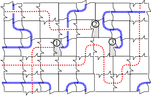
Refer to caption Refer to caption (A) (D) Refer to caption Refer to caption (B) (E) Refer to caption Refer to caption (C) (F)

Figure 1: (A) A gap in ℑ​𝔠​𝔢\mathfrak{I{\scriptstyle\!ce}}; see Examples 1.1(a) and 2.3(a). (B,C) Gaps in 𝔇​𝔬​𝔪\mathfrak{D{\scriptstyle\!om}}; see Examples 1.1(b) and 2.3(b,c). (D) A ‘pole’ in ℑ​𝔠​𝔢\mathfrak{I{\scriptstyle\!ce}}; see Examples 1.1(a) and 2.2(a). (E) Three ‘poles’ in 𝔓​𝔱​𝔥\mathfrak{P{\scriptstyle\!th}}; see Examples 1.1(d) and 2.2(b). (F) A non-pole in 𝔇​𝔬​𝔪\mathfrak{D{\scriptstyle\!om}}; see Examples 1.1(b) and 2.2(c).
  • Example 1.5: (a) (Square ice) Let ℐ={[Uncaptioned image]}{\mathcal{I}}=\left\{\raisebox{-5.0pt}{\includegraphics[scale]{Pictures/Ice/ice0.eps}}\right\}, and let ℑ​𝔠​𝔢⊂ℐℤ2\mathfrak{I{\scriptstyle\!ce}}\subset{\mathcal{I}}^{{{\mathbb{Z}}^{2}}} be the Wang subshift defined by the obvious edge-matching conditions. Figure 1(A) shows a domain boundary in ℑ​𝔠​𝔢\mathfrak{I{\scriptstyle\!ce}}. See also Example 2.3(a).

    (b) (Domino Tiling) Let 𝒟:={ [Uncaptioned image]}{\mathcal{D}}:=\left\{\raisebox{-5.0pt}{ \includegraphics[scale]{Pictures/Dominoes/dominoes.eps}}\right\}, and let 𝔇​𝔬​𝔪⊂𝒟ℤ2\mathfrak{D{\scriptstyle\!om}}\subset{\mathcal{D}}^{{{\mathbb{Z}}^{2}}} be the Wang subshift defined by the obvious edge-matching conditions. Figure 1(B,C) shows two domain boundaries in 𝔇​𝔬​𝔪\mathfrak{D{\scriptstyle\!om}}; see also Example 2.3(b,c).

    (c) (Ice cubes) Let 𝒬{\mathcal{Q}} be the set of twenty ‘ball-and-pin’ structures in Figure 2(A), and let 𝔔⊂𝒬ℤ3{\mathfrak{Q}}\subset{\mathcal{Q}}^{{{\mathbb{Z}}^{3}}} be the Wang subshift defined by the obvious matching conditions (this is a three-dimensional version of ‘square ice’). Figure 2(B) shows a domain boundary in 𝔔{\mathfrak{Q}}. ♢\diamondsuit

For any 𝗓∈ℤD{\mathsf{z}}\in{{\mathbb{Z}}^{D}}, let :=⌟⌜𝗓⌝𝗓+[0,1]D{}^{\ulcorner}_{{\mathsf{z}}}{\ }{}^{\urcorner}_{\lrcorner}:={\mathsf{z}}+{\left[0,1\right]}^{D}; hence ⌜𝗓⌝⌟{}^{\ulcorner}_{{\mathsf{z}}}{\ }{}^{\urcorner}_{\lrcorner} is a unit cube with one corner at 𝗓{\mathsf{z}}, and the other corners at adjacent points in ℤD{{\mathbb{Z}}^{D}}. Let 𝕂𝗓⊂ℤD{\mathbb{K}}_{\mathsf{z}}\subset{{\mathbb{Z}}^{D}} be the set of corner points of ⌜𝗓⌝⌟{}^{\ulcorner}_{{\mathsf{z}}}{\ }{}^{\urcorner}_{\lrcorner}. We adopt the following notational convention: if 𝕐⊂ℤD{\mathbb{Y}}\subset{{\mathbb{Z}}^{D}} is any subset, then let 𝐘{\mathbf{Y}} be the minimal closed subset of ℝD{{\mathbb{R}}^{D}} containing 𝕐{\mathbb{Y}} and all unit cubes whose corners are in 𝕐{\mathbb{Y}}. Formally:

𝐘:=⋃𝗓∈ℤD&𝕂𝗓⊂𝕐⌜𝗓⌝⌟{\mathbf{Y}}\quad:=\quad\bigcup_{{\mathsf{z}}\in{{\mathbb{Z}}^{D}}\ \&\ {\mathbb{K}}_{\mathsf{z}}\subset{\mathbb{Y}}}{}^{\ulcorner}_{{\mathsf{z}}}{\ }{}^{\urcorner}_{\lrcorner}

It follows that 𝕐{\mathbb{Y}} is trail-connected iff 𝐘{\mathbf{Y}} is path-connected. In this case, for any k∈[2​…​D]k\in{\left[2...D\right]}, we define the kkth homotopy group πk​(𝕐,𝗒):=πk​(𝐘,𝗒)\pi_{k}({\mathbb{Y}},{\mathsf{y}}):=\pi_{k}({\mathbf{Y}},{\mathsf{y}}), for some fixed basepoint 𝗒∈𝕐{\mathsf{y}}\in{\mathbb{Y}} (different choices of 𝗒{\mathsf{y}} yield isomorphic groups); see [Hat02, §4.1]. If 𝐚∈𝔄~{\mathbf{a}}\in\widetilde{{\mathfrak{A}}}, and r>0r>0, then 𝐚{\mathbf{a}} has a range rr codimension-kk defect if πk−1​(𝔾r​(𝐚),𝗒)\pi_{k-1}({\mathbb{G}}_{r}({\mathbf{a}}),{\mathsf{y}}) is nontrivial for some 𝗒∈𝔾r​(𝐚){\mathsf{y}}\in{\mathbb{G}}_{r}({\mathbf{a}}). If 𝔾r​(𝐚){\mathbb{G}}_{r}({\mathbf{a}}) is disconnected (e.g. by a domain boundary) then different connected components may have different homotopy groups; we only require one of these to be nontrivial.

  • Example 1.6: (a) Let ℑ​𝔠​𝔢\mathfrak{I{\scriptstyle\!ce}} be as in Example 1.1(a). Then Figure 1(D) shows a codimension-two defect in ℑ​𝔠​𝔢\mathfrak{I{\scriptstyle\!ce}}. See also Example 2.2(a).

    (b) Let 𝔇​𝔬​𝔪\mathfrak{D{\scriptstyle\!om}} as in Example 1.1(b). Then Figure 1(F) shows a codimension-two defect in 𝔇​𝔬​𝔪\mathfrak{D{\scriptstyle\!om}}. See also Example 2.2(c).

    (c) Let 𝔔{\mathfrak{Q}} be as in Example 1.1(c). Figure 2(C) shows a codimension-two defect in 𝔔{\mathfrak{Q}}, and Figure 2(D) shows a codimension-three defect.

    𝒫:={[Uncaptioned image]}.{\mathcal{P}}\ :=\ \left\{\raisebox{26.00009pt}{\includegraphics[scale,angle]{Pictures/Path/path0.eps}}\right\}.

    (d) (Two-coloured, undirected, crossing path tiling) Let 𝒫{\mathcal{P}} be the set of 21 tiles shown above, and let 𝔓​𝔱​𝔥⊂𝒫ℤ2\mathfrak{P{\scriptstyle\!th}}\subset{\mathcal{P}}^{{{\mathbb{Z}}^{2}}} be the Wang subshift defined by the obvious edge-matching conditions. Then 𝔓​𝔱​𝔥\mathfrak{P{\scriptstyle\!th}}-admissible configurations are tangles of undirected, freely crossing paths in two colours [Ein01, §3]. Figure 1(E) shows three codimension-two defects in 𝔓​𝔱​𝔥\mathfrak{P{\scriptstyle\!th}}. See also Example 2.2(b). ♢\diamondsuit

Refer to caption

Figure 2: (A) The twenty tiles of the ‘ice cube’ shift 𝔔⊂𝒬ℤ3{\mathfrak{Q}}\subset{\mathcal{Q}}^{{{\mathbb{Z}}^{3}}} from Examples 1.1(c) and 1.1(c). (B) A domain boundary in 𝔔{\mathfrak{Q}}; we assume that the same pattern is continued up, down, north, and south. (We have ‘stretched out’ the configuration for visibility. The balls in the defect region are shaded, but left unspecified, because they don’t matter.) (C) A codimension-two defect in 𝔔{\mathfrak{Q}}; we assume that the same pattern is continued upwards and downwards. (D) A codimension-three (‘pole’) defect in 𝔔{\mathfrak{Q}}; see also Example 4.1(b).

1.2 Proper homotopy and projective codimension:

Let 𝐗{\mathbf{X}} be a topological space and let x∈𝐗x\in{\mathbf{X}}. Let 𝕊k⊂ℝk+1{\mathbb{S}}^{k}\subset{{\mathbb{R}}^{k+1}} be the unit kk-sphere, and let s∈𝕊ks\in{\mathbb{S}}^{k} be some distinguished point. We write α:(𝕊k,s)⟶(𝐗,x)\alpha:({\mathbb{S}}^{k},s){{\longrightarrow}}({\mathbf{X}},x) to mean α\alpha is a continuous function from 𝕊k{\mathbb{S}}^{k} into 𝐗{\mathbf{X}} and f⁡(s)=xf(s)=x. If α,β:(𝕊k,s)⟶(𝐗,x)\alpha,\beta:({\mathbb{S}}^{k},s){{\longrightarrow}}({\mathbf{X}},x) then we write α≈β\alpha\approx\beta to mean that α\alpha is homotopic to β\beta in a manner which always maps ss to xx; we call this a basepoint-fixing homotopy (where xx is the basepoint). We then use α¯{\underline{\alpha}} to refer to the (basepoint-fixing) homotopy class of α\alpha.

If β:[0,1]⟶𝐗\beta:{\left[0,1\right]}{{\longrightarrow}}{\mathbf{X}}, then β←:[0,1]⟶𝐗\stackrel{{\scriptstyle\leftarrow}}{{\beta}}\!:{\left[0,1\right]}{{\longrightarrow}}{\mathbf{X}} is defined by β←(t)=β⁡(1−t)\stackrel{{\scriptstyle\leftarrow}}{{\beta}}\!(t)=\beta(1-t). If α:[0,1]⟶𝐗\alpha:{\left[0,1\right]}{{\longrightarrow}}{\mathbf{X}}, and β⁡(0)=α⁡(1)\beta(0)=\alpha(1), then let α⋆β:[0,1]⟶𝐗\alpha\star\beta:{\left[0,1\right]}{{\longrightarrow}}{\mathbf{X}} be the concatenation of α\alpha and β\beta (i.e. α⋆β⁡(t):=α⁡(2​t)\alpha\star\beta(t):=\alpha(2t) if t∈[0,12]t\in{\left[0,\frac{1}{2}\right]} and α⋆β⁡(t):=β⁡(2​t−1)\alpha\star\beta(t):=\beta(2t-1) if t∈[12,1]t\in{\left[\frac{1}{2},1\right]}). Thus, π1​(𝐗,x)\pi_{1}({\mathbf{X}},x) is the group of all homotopy classes of loops α:[0,1]⟶𝐗\alpha:{\left[0,1\right]}{{\longrightarrow}}{\mathbf{X}} with α⁡(0)=x=α⁡(1)\alpha(0)=x=\alpha(1), with operation α¯⋅β¯:=α⋆β¯{\underline{\alpha}}\cdot{\underline{\beta}}:=\underline{\alpha\star\beta} [Hat02, §1.1]. We can also treat the elements of π1​(𝐗,x)\pi_{1}({\mathbf{X}},x) as homotopy classes of functions α:(𝕊1,s)⟶(𝐗,x)\alpha:({\mathbb{S}}^{1},s){{\longrightarrow}}({\mathbf{X}},x). By generalizing this construction, we can define an abelian group πk​(𝐗,x)\pi_{k}({\mathbf{X}},x) of homotopy classes of functions α:(𝕊k,s)⟶(𝐗,x)\alpha:({\mathbb{S}}^{k},s){{\longrightarrow}}({\mathbf{X}},x). See [Hat02, §4.1] for details.

Let x,y∈𝐗x,y\in{\mathbf{X}}. If β:[0,1]⟶𝐗\beta:{\left[0,1\right]}{{\longrightarrow}}{\mathbf{X}} is any path with with β⁡(0)=x\beta(0)=x and β⁡(1)=y\beta(1)=y, then β\beta yields an isomorphism β∗:π1​(𝐗,x)⟶π1​(𝐗,y)\beta_{*}:\pi_{1}({\mathbf{X}},x){{\longrightarrow}}\pi_{1}({\mathbf{X}},y) by β∗​(α¯):=β⋆α⋆β←¯\beta_{*}({\underline{\alpha}}):=\underline{\beta\star\alpha\star\stackrel{{\scriptstyle\leftarrow}}{{\beta}}\!}. We can likewise use β\beta to define isomorphisms β∗:πk​(𝐗,x)⟶πk​(𝐗,y)\beta_{*}:\pi_{k}({\mathbf{X}},x){{\longrightarrow}}\pi_{k}({\mathbf{X}},y) for all k≥2k\geq 2. If γ:[0,1]⟶𝐗\gamma:{\left[0,1\right]}{{\longrightarrow}}{\mathbf{X}} is another path from xx to yy, and γ≈β\gamma\approx\beta, then γ∗=β∗\gamma_{*}=\beta_{*}. However, if γ\gamma is not homotopic to β\beta, then γ∗\gamma_{*} and β∗\beta_{*} may be different. Hence, although πk​(𝐗,x)≅πk​(𝐗,y)\pi_{k}({\mathbf{X}},x)\cong\pi_{k}({\mathbf{X}},y), this isomorphism is not ‘canonical’.

Let 𝔄⊂𝒜ℤD{\mathfrak{A}}\subset{\mathcal{A}}^{{{\mathbb{Z}}^{D}}} be a subshift and let 𝐚∈𝔄~{\mathbf{a}}\in\widetilde{{\mathfrak{A}}}, and suppose, for some r0∈ℕr_{0}\in{\mathbb{N}}, that 𝔾r0​(𝐚){\mathbb{G}}_{r_{0}}({\mathbf{a}}) contains a unique projective connected component 𝕐{\mathbb{Y}} (it is necessary, but not sufficient, to assume that 𝐚{\mathbf{a}} has no projective domain boundaries). Thus, for all r>r0r>r_{0}, 𝕐r:=𝕐∩𝔾r​(𝐚){\mathbb{Y}}_{r}:={\mathbb{Y}}\cap{\mathbb{G}}_{r}({\mathbf{a}}) is the unique projective component of 𝔾r​(𝐚){\mathbb{G}}_{r}({\mathbf{a}}). A proper base ray is a continuous path ω:[0,∞)⟶𝐘r0\omega:{\left[0,{\infty}\right)}{{\longrightarrow}}{\mathbf{Y}}_{r_{0}} with limt→∞|ω⁡(t)|=∞\lim_{t{\rightarrow}{\infty}}|\omega(t)|={\infty}. For each r>r0r>r_{0}, we define πk​(𝕐r,ω):=πk​(𝕐r,𝗒)\pi_{k}({\mathbb{Y}}_{r},\omega):=\pi_{k}({\mathbb{Y}}_{r},{\mathsf{y}}), where 𝗒∈𝕐r∩ω[0,∞){\mathsf{y}}\in{\mathbb{Y}}_{r}\cap\omega{\left[0,{\infty}\right)} is any point. This definition is independent of the choice of 𝗒{\mathsf{y}} in the following sense: if 𝗒′∈𝕐r∩ω[0,∞){\mathsf{y}}^{\prime}\in{\mathbb{Y}}_{r}\cap\omega{\left[0,{\infty}\right)} is another point, then there is a canonical isomorphism πk​(𝕐r,𝗒)≅πk​(𝕐r,𝗒′)\pi_{k}({\mathbb{Y}}_{r},{\mathsf{y}})\cong\pi_{k}({\mathbb{Y}}_{r},{\mathsf{y}}^{\prime}) given by the segment of ω\omega between 𝗒{\mathsf{y}} and 𝗒′{\mathsf{y}}^{\prime}.

Recall that 𝕐r+1⊂𝕐r{\mathbb{Y}}_{r+1}\subset{\mathbb{Y}}_{r}; the inclusion map ιr:𝕐r+1↪𝕐r\iota_{r}:{\mathbb{Y}}_{r+1}\hookrightarrow{\mathbb{Y}}_{r} yields a (canonical) homomorphism ιr∗:πk​(𝕐r+1,ω)⟶πk​(𝕐r,ω)\iota_{r}^{*}:\pi_{k}({\mathbb{Y}}_{r+1},\omega){{\longrightarrow}}\pi_{k}({\mathbb{Y}}_{r},\omega). We define the kkth proper homotopy group to be the inverse limit:

πk​(𝔾∞​(𝐚),ω):=lim⟵(πk​(𝕐1,ω)⟵⁣−ι1∗πk​(𝕐2,ω)⟵⁣−ι2∗πk​(𝕐3,ω)⟵⁣−ι3∗⋯)\pi_{k}({\mathbb{G}}_{{\infty}}({\mathbf{a}}),\omega)\quad:=\quad\lim_{\longleftarrow}\left(\pi_{k}({\mathbb{Y}}_{1},\omega)\stackrel{{\scriptstyle\iota^{*}_{1}}}{{\longleftarrow\!\!\!-}}\pi_{k}({\mathbb{Y}}_{2},\omega)\stackrel{{\scriptstyle\iota^{*}_{2}}}{{\longleftarrow\!\!\!-}}\pi_{k}({\mathbb{Y}}_{3},\omega)\stackrel{{\scriptstyle\iota^{*}_{3}}}{{\longleftarrow\!\!\!-}}\cdots\right) (1)

(Of course “πk​(𝔾∞​(𝐚))\pi_{k}({\mathbb{G}}_{{\infty}}({\mathbf{a}}))” is an abuse of notation, because technically, 𝔾∞​(𝐚)=∅{\mathbb{G}}_{{\infty}}({\mathbf{a}})=\emptyset. See [Hat02, §3.F] or [Lan84, §III.9] for background on inverse limits. The group πk​(𝔾∞​(𝐚),ω)\pi_{k}({\mathbb{G}}_{{\infty}}({\mathbf{a}}),\omega) is analogous (but not identical) to the proper homotopy group of a noncompact topological space; see [Bro74], [BT74] or [Pes90, §2].) We say that 𝐚{\mathbf{a}} has projective codimension (k+1)(k+1) defect if πk​[𝔾∞​(𝐚),ω]\pi_{k}[{\mathbb{G}}_{{\infty}}({\mathbf{a}}),\omega] is nontrivial (it follows that πk​[𝔾r​(𝐚),ω]\pi_{k}[{\mathbb{G}}_{r}({\mathbf{a}}),\omega] is nontrivial for all large enough r∈ℕr\in{\mathbb{N}}). Heuristically, elements of πk​(𝔾∞​(𝐚))\pi_{k}({\mathbb{G}}_{{\infty}}({\mathbf{a}})) are homotopy classes of ‘extremely large’ kk-sphere embeddings in the unflawed part of 𝐚{\mathbf{a}}. Technically, this definition depends upon the homotopy class of the proper base ray ω\omega; different rays may yield nonisomorphic groups.

2 Cohomological Defects

The main results of this section are Theorems 2.8 and 2.15 and Proposition 2.11.

2.1 Dynamical Cocycles

Let 𝔄⊆𝒜ℤD{\mathfrak{A}}\subseteq{\mathcal{A}}^{{{\mathbb{Z}}^{D}}} be a subshift, and let (𝒢,⋅)({\mathcal{G}},\cdot) be a topological group (usually discrete). A 𝒢{\mathcal{G}}-valued continuous (dynamical) cocycle for 𝔄{\mathfrak{A}} is a continuous function C:ℤD×𝔄⟶𝒢C:{{\mathbb{Z}}^{D}}\times{\mathfrak{A}}{{\longrightarrow}}{\mathcal{G}} satisfying the cocycle equation

C⁡(𝗒+𝗓,𝐚)=C⁡(𝗒,σ𝗓​(𝐚))⋅C⁡(𝗓,𝐚),∀𝐚∈𝒜ℤD​ and ​∀𝗒,𝗓∈ℤD.C({\mathsf{y}}+{\mathsf{z}},{\mathbf{a}})\quad=\quad C({\mathsf{y}},\sigma^{{\mathsf{z}}}({\mathbf{a}}))\cdot C({\mathsf{z}},{\mathbf{a}}),\qquad\forall\,{\mathbf{a}}\in{\mathcal{A}}^{{{\mathbb{Z}}^{D}}}\mbox{\ and \ }\forall\,{\mathsf{y}},{\mathsf{z}}\in{{\mathbb{Z}}^{D}}. (2)
  • Example 2.1: (a) If b:𝔄⟶𝒢b:{\mathfrak{A}}{{\longrightarrow}}{\mathcal{G}} is any continuous function, then the function C⁡(𝗓,𝐚):=b⁡(σ𝗓​(𝐚))⋅b​(𝐚)−1C({\mathsf{z}},{\mathbf{a}}):=b(\sigma^{{\mathsf{z}}}({\mathbf{a}}))\cdot b({\mathbf{a}})^{-1} is a cocycle, and is called a coboundary with cobounding function bb.

    (b) If h:ℤD⟶𝒢h:{{\mathbb{Z}}^{D}}{{\longrightarrow}}{\mathcal{G}} is a homomorphism, then the function C⁡(𝗓,𝐚):=h⁡(𝗓)C({\mathsf{z}},{\mathbf{a}}):=h({\mathsf{z}}) is a cocycle. Conversely, if CC is any cocycle such that C⁡(𝗓,¯)C({\mathsf{z}},\underline{\ \ }) is constant for all 𝗓∈ℤD{\mathsf{z}}\in{{\mathbb{Z}}^{D}}, then CC arises from a homomorphism in this manner. In particular, if e𝒢∈𝒢e_{\mathcal{G}}\in{\mathcal{G}} is the identity, then the constant function Ce​(𝗓,𝐚)≡e𝒢C_{e}({\mathsf{z}},{\mathbf{a}})\equiv e_{\mathcal{G}} is a cocycle.

    (c) Let ℑ​𝔠​𝔢⊂ℐℤ2\mathfrak{I{\scriptstyle\!ce}}\subset{\mathcal{I}}^{{{\mathbb{Z}}^{2}}} be as in Example 1.1(a). Define c1,c2:ℐ⟶{±1}c_{1},c_{2}:{\mathcal{I}}{{\longrightarrow}}\{\pm 1\} by c1​(⌜∗⌝∗∗⌞[Uncaptioned image]⌟):=+1=:c2​(⌜∗⌝[Uncaptioned image] ∗⌞∗⌟)c_{1}(\mbox{\tiny$\begin{array}[]{rcl}{}_{\ulcorner}&\!\!\!\!\!\!\mbox{\scriptsize$*$}&\!{}_{\urcorner}\\ \mbox{\scriptsize$*$}&&\!\mbox{\scriptsize$*$}\\ {}^{\llcorner}&\!\!\!\!\!\!\mbox{\scriptsize$\hbox{\includegraphics[scale]{Pictures/Ice/sqn.eps}}$}&\!{}^{\lrcorner}\end{array}$}):=+1=:c_{2}(\mbox{\tiny$\begin{array}[]{rcl}{}_{\ulcorner}&\!\!\!\!\!\!\mbox{\scriptsize$*$}&\!{}_{\urcorner}\\ \mbox{\scriptsize$\hbox{\raisebox{-1.99997pt}{\includegraphics[scale]{Pictures/Ice/sqw.eps}}}\,\ $}&&\!\mbox{\scriptsize$*$}\\ {}^{\llcorner}&\!\!\!\!\!\!\mbox{\scriptsize$*$}&\!{}^{\lrcorner}\end{array}$}) and c1​(⌜∗⌝∗∗⌞[Uncaptioned image]⌟):=−1=:c2​(⌜∗⌝ [Uncaptioned image]∗⌞∗⌟)c_{1}(\mbox{\tiny$\begin{array}[]{rcl}{}_{\ulcorner}&\!\!\!\!\!\!\mbox{\scriptsize$*$}&\!{}_{\urcorner}\\ \mbox{\scriptsize$*$}&&\!\mbox{\scriptsize$*$}\\ {}^{\llcorner}&\!\!\!\!\!\!\mbox{\scriptsize$\hbox{\raisebox{-1.99997pt}{\includegraphics[scale]{Pictures/Ice/sqs.eps}}}$}&\!{}^{\lrcorner}\end{array}$}):=-1=:c_{2}(\mbox{\tiny$\begin{array}[]{rcl}{}_{\ulcorner}&\!\!\!\!\!\!\mbox{\scriptsize$*$}&\!{}_{\urcorner}\\ \mbox{\scriptsize$\,\hbox{\raisebox{-1.99997pt}{\includegraphics[scale]{Pictures/Ice/sqe.eps}}}$}&&\!\mbox{\scriptsize$*$}\\ {}^{\llcorner}&\!\!\!\!\!\!\mbox{\scriptsize$*$}&\!{}^{\lrcorner}\end{array}$}) (‘∗*’ means ‘anything’). We define cocycle C:ℤ2×ℑ​𝔠​𝔢⟶ℤC:{{\mathbb{Z}}^{2}}\times\mathfrak{I{\scriptstyle\!ce}}{{\longrightarrow}}{\mathbb{Z}} as follows: If 𝐢∈ℑ​𝔠​𝔢{\mathbf{i}}\in\mathfrak{I{\scriptstyle\!ce}} and 𝗓=(z1,z2)∈ℤ2{\mathsf{z}}=(z_{1},z_{2})\in{{\mathbb{Z}}^{2}}, then

    C⁡(𝗓,𝐢):=∑x=0z1−1c1​(ix,0)+∑y=0z2−1c2​(iz1,y).C({\mathsf{z}},{\mathbf{i}})\quad:=\quad\sum_{x=0}^{z_{1}-1}c_{1}(i_{x,0})+\sum_{y=0}^{z_{2}-1}c_{2}(i_{z_{1},y}). (3)

    (d) Let 𝔓​𝔱​𝔥⊂𝒫ℤ2\mathfrak{P{\scriptstyle\!th}}\subset{\mathcal{P}}^{{{\mathbb{Z}}^{2}}} be as in Example 1.1(d). Define c1,c2:ℐ⟶ℤ/2⊕ℤ/2c_{1},c_{2}:{\mathcal{I}}{{\longrightarrow}}{{\mathbb{Z}}_{/2}}\oplus{{\mathbb{Z}}_{/2}} by c1​( [Uncaptioned image]):=(1,0)=:c2​([Uncaptioned image])c_{1}(\hbox{\,\raisebox{-6.99997pt}{\includegraphics[scale]{Pictures/Path/westbluepath.eps}}$\!$}):=(1,0)=:c_{2}(\hbox{\raisebox{-5.0pt}{\includegraphics[scale]{Pictures/Path/southbluepath.eps}}}) and c1​( [Uncaptioned image]):=(0,1)=:c2​([Uncaptioned image])c_{1}(\hbox{\,\raisebox{-6.99997pt}{\includegraphics[scale]{Pictures/Path/westredpath.eps}}$\!$}):=(0,1)=:c_{2}(\hbox{\raisebox{-5.0pt}{\includegraphics[scale]{Pictures/Path/southredpath.eps}}}) (where ‘∗*’ means ‘anything’), and extend this to a cocycle C:ℤ2×𝔓​𝔱​𝔥⟶ℤ/2⊕ℤ/2C:{{\mathbb{Z}}^{2}}\times\mathfrak{P{\scriptstyle\!th}}{{\longrightarrow}}{{\mathbb{Z}}_{/2}}\oplus{{\mathbb{Z}}_{/2}} exactly as in eqn.(3).

    (e) More generally, a height function is any integer-valued11 1 Sometimes HH maps into ℤn{\mathbb{Z}}^{n} [She02] or other groups [KK93], and the ‘height’ metaphor is somewhat strained. cocycle H:ℤD×𝔄⟶ℤH:{{\mathbb{Z}}^{D}}\times{\mathfrak{A}}{{\longrightarrow}}{\mathbb{Z}} defined by functions h1,…,hD:𝒜⟶ℤh_{1},\ldots,h_{D}:{\mathcal{A}}{{\longrightarrow}}{\mathbb{Z}} via the obvious generalization of eqn.(3). Height functions appear in tiling systems like dominos [CEP96, CKP01] and ‘ice’ tiles [Elo99, Elo03, Elo05], and in many lattice models of statistical physics [Bax89].

    (f) Let 𝔇​𝔬​𝔪⊂𝒟ℤ2\mathfrak{D{\scriptstyle\!om}}\subset{\mathcal{D}}^{{{\mathbb{Z}}^{2}}} be as in Example 1.1(b). Let 𝒢:=ℤ/2∗ℤ/2{\mathcal{G}}:={{\mathbb{Z}}_{/2}}*{{\mathbb{Z}}_{/2}} be the group of finite products like vhvhv⋯vhvvhvhv\cdots vhv, where vv and hh are noncommuting generators with v2=e=h2v^{2}=e=h^{2}. Define c1,c2:ℐ⟶𝒢c_{1},c_{2}:{\mathcal{I}}{{\longrightarrow}}{\mathcal{G}} by

    c1​(⌜−⌝||⌞[Uncaptioned image]⌟):=v​h​v;c1​(⌜∗⌝∗∗⌞−⌟):=h;c2​(⌜−⌝ [Uncaptioned image]|⌞−⌟):=h​v​h,and​c2​(⌜∗⌝|∗⌞∗⌟):=vc_{1}(\mbox{\tiny$\begin{array}[]{rcl}{}_{\ulcorner}&\!\!\!\!\!\!\mbox{\scriptsize$-$}&\!{}_{\urcorner}\\ \mbox{\scriptsize$|\ $}&&\!\mbox{\scriptsize$\,|$}\\ {}^{\llcorner}&\!\!\!\!\!\!\mbox{\scriptsize$\hbox{\includegraphics[scale]{Pictures/Ice/sqn.eps}}$}&\!{}^{\lrcorner}\end{array}$}):=vhv;\quad c_{1}(\mbox{\tiny$\begin{array}[]{rcl}{}_{\ulcorner}&\!\!\!\!\!\!\mbox{\scriptsize$*$}&\!{}_{\urcorner}\\ \mbox{\scriptsize$*$}&&\!\mbox{\scriptsize$*$}\\ {}^{\llcorner}&\!\!\!\!\!\!\mbox{\scriptsize$-$}&\!{}^{\lrcorner}\end{array}$}):=h;\quad c_{2}(\mbox{\tiny$\begin{array}[]{rcl}{}_{\ulcorner}&\!\!\!\!\!\!\mbox{\scriptsize$-$}&\!{}_{\urcorner}\\ \mbox{\scriptsize$\,\hbox{\raisebox{-1.99997pt}{\includegraphics[scale]{Pictures/Ice/sqe.eps}}}$}&&\!\mbox{\scriptsize$\,|$}\\ {}^{\llcorner}&\!\!\!\!\!\!\mbox{\scriptsize$-$}&\!{}^{\lrcorner}\end{array}$}):=hvh;\ \mbox{and}\ c_{2}(\mbox{\tiny$\begin{array}[]{rcl}{}_{\ulcorner}&\!\!\!\!\!\!\mbox{\scriptsize$*$}&\!{}_{\urcorner}\\ \mbox{\scriptsize$|\ $}&&\!\mbox{\scriptsize$*$}\\ {}^{\llcorner}&\!\!\!\!\!\!\mbox{\scriptsize$*$}&\!{}^{\lrcorner}\end{array}$}):=v.

    and extend this to a cocycle C:ℤ2×𝔇​𝔬​𝔪⟶𝒢C:{{\mathbb{Z}}^{2}}\times\mathfrak{D{\scriptstyle\!om}}{{\longrightarrow}}{\mathcal{G}} through the multiplicative analogy of eqn.(3).

    (g) If 𝒳{\mathcal{X}} is a topological space, then an 𝒳{\mathcal{X}}-extension of 𝔄{\mathfrak{A}} is a continuous ℤD{{\mathbb{Z}}^{D}}-action Ξ:ℤD×𝒳×𝔄⟶𝒳×𝔄\Xi:{{\mathbb{Z}}^{D}}\times{\mathcal{X}}\times{\mathfrak{A}}{{\longrightarrow}}{\mathcal{X}}\times{\mathfrak{A}} such that (𝔄,σ)({\mathfrak{A}},\sigma) is a factor of (𝒳×𝔄,Ξ)({\mathcal{X}}\times{\mathfrak{A}},\Xi) via the projection π𝔄:𝒳×𝔄↠𝔄\pi_{\mathfrak{A}}:{\mathcal{X}}\times{\mathfrak{A}}\twoheadrightarrow{\mathfrak{A}}. Let 𝒢:=H​omeo​(𝒳){\mathcal{G}}:=\mathrm{H\scriptstyle{omeo}}({\mathcal{X}}) be the self-homeomorphism group of 𝒳{\mathcal{X}}, topologized as a subspace of the Tychonoff product 𝒳𝒳{\mathcal{X}}^{\mathcal{X}} (e.g. if 𝒳:=[1​…​n]{\mathcal{X}}:={\left[1...n\right]}, then 𝒢=𝐒n{\mathcal{G}}={\mathbf{S}}_{n} is a (discrete) permutation group; this is called an nn-point extension). For each 𝐚∈𝔄{\mathbf{a}}\in{\mathfrak{A}} and 𝗓∈ℤD{\mathsf{z}}\in{{\mathbb{Z}}^{D}}, let c⁡(𝗓,𝐚):=π𝒳∘Ξ𝗓​(¯,𝐚):𝒳⟶𝒳c({\mathsf{z}},{\mathbf{a}}):=\pi_{\mathcal{X}}\circ\Xi^{\mathsf{z}}(\underline{\ \ },{\mathbf{a}}):{\mathcal{X}}{{\longrightarrow}}{\mathcal{X}}. Then c:ℤD×𝔄⟶𝒢c:{{\mathbb{Z}}^{D}}\times{\mathfrak{A}}{{\longrightarrow}}{\mathcal{G}} is a continuous cocycle. Conversely, any continuous cocycle c:ℤD×𝔄⟶𝒢c:{{\mathbb{Z}}^{D}}\times{\mathfrak{A}}{{\longrightarrow}}{\mathcal{G}} defines an 𝒳{\mathcal{X}}-extension of 𝔄{\mathfrak{A}} in the obvious way; see e.g. [Zim76, Zim77, Zim80, Kam90, Kam92, Kam93]. ♢\diamondsuit

Two continuous cocycles CC and C′C^{\prime} are cohomologous (C≈C′C\approx C^{\prime}) if there is a continuous transfer function b:𝔄⟶𝒢b:{\mathfrak{A}}{{\longrightarrow}}{\mathcal{G}} such that C′​(𝗓,𝐚)=b⁡(σ𝗓​(𝐚))⋅C⁡(𝗓,𝐚)⋅b​(𝐚)−1C^{\prime}({\mathsf{z}},{\mathbf{a}})\ =\ b(\sigma^{{\mathsf{z}}}({\mathbf{a}}))\cdot C({\mathsf{z}},{\mathbf{a}})\cdot b({\mathbf{a}})^{-1}, for all 𝗓∈ℤD{\mathsf{z}}\in{{\mathbb{Z}}^{D}} and 𝐚∈𝔄{\mathbf{a}}\in{\mathfrak{A}}. A cocycle CC is trivial if CC is cohomologous to a homomorphism. We will use C¯{\underline{C}} to denote the cohomology equivalence class of the cocycle CC.

  • Example 2.2: (a) Any coboundary [Example 2.1(a)] is trivial, because it is cohomologous to the homomorphism CeC_{e} [Example 2.1(b)].

    (b) Fix 𝗒∈ℤD{\mathsf{y}}\in{{\mathbb{Z}}^{D}} and define cocycle C′​(𝗓,𝐚):=C⁡(𝗓,σ𝗒​(𝐚))C^{\prime}({\mathsf{z}},{\mathbf{a}}):=C({\mathsf{z}},\sigma^{{\mathsf{y}}}({\mathbf{a}})). Then C≈C′C\approx C^{\prime} via the transfer function b⁡(𝐚):=C⁡(𝗒,𝐚)b({\mathbf{a}}):=C({\mathsf{y}},{\mathbf{a}}).

    (c) Let Ξ,Ξ′:ℤD×𝒳×𝔄⟶𝒳×𝔄\Xi,\Xi^{\prime}:{{\mathbb{Z}}^{D}}\times{\mathcal{X}}\times{\mathfrak{A}}{{\longrightarrow}}{\mathcal{X}}\times{\mathfrak{A}} be two 𝒳{\mathcal{X}}-extensions of 𝔄{\mathfrak{A}}, with cocycles C,C′:ℤD×𝔛⟶𝒢:=H​omeo​(𝒳)C,C^{\prime}:{{\mathbb{Z}}^{D}}\times{\mathfrak{X}}{{\longrightarrow}}{\mathcal{G}}:=\mathrm{H\scriptstyle{omeo}}({\mathcal{X}}) as in Example 2.1(g). Then C≈C′C\approx C^{\prime} via the continuous transfer function b:𝔄⟶𝒢b:{\mathfrak{A}}{{\longrightarrow}}{\mathcal{G}} iff the systems (𝒳×𝔄,Ξ)({\mathcal{X}}\times{\mathfrak{A}},\Xi) and (𝒳×𝔄,Ξ′)({\mathcal{X}}\times{\mathfrak{A}},\Xi^{\prime}) are conjugate via the function (x,𝐚)↦(b⁡(𝐚)​(x),𝐚)(x,{\mathbf{a}})\mapsto(b({\mathbf{a}})(x),{\mathbf{a}}). Also, CC is a homomorphism iff there is a continuous ℤD{{\mathbb{Z}}^{D}}-action ξ\xi on 𝒳{\mathcal{X}} such that (𝒳×𝔄,Ξ)=(𝒳,ξ)×(𝔄,σ)({\mathcal{X}}\times{\mathfrak{A}},\Xi)=({\mathcal{X}},\xi)\times({\mathfrak{A}},\sigma) [i.e. C⁡(𝗓,𝐚)=ξ𝗓C({\mathsf{z}},{\mathbf{a}})=\xi^{\mathsf{z}}, for all 𝐚∈𝔄{\mathbf{a}}\in{\mathfrak{A}}]. Hence, CC is trivial iff (𝒳×𝔄,Ξ)({\mathcal{X}}\times{\mathfrak{A}},\Xi) is isomorphic to such a Cartesian product. ♢\diamondsuit

If (𝒢,⋅)({\mathcal{G}},\cdot) is an abelian group, then the set 𝒵=𝒵dy1(𝔄,𝒢){\mathcal{Z}}={\mathcal{Z}}_{{}^{\mathrm{dy}}}^{1}({\mathfrak{A}},{\mathcal{G}}) of all 𝒢{\mathcal{G}}-valued continuous cocycles is a group under pointwise multiplication. The set of trivial cocycles is a subgroup ℬ=ℬdy1(𝔄,𝒢){\mathcal{B}}={\mathcal{B}}_{{}^{\mathrm{dy}}}^{1}({\mathfrak{A}},{\mathcal{G}}). The quotient group ℋdy1(𝔄,𝒢):=𝒵/ℬ{\mathcal{H}}_{{}^{\mathrm{dy}}}^{1}({\mathfrak{A}},{\mathcal{G}}):={\mathcal{Z}}/{\mathcal{B}} is the (first dynamical) cohomology group of 𝔄{\mathfrak{A}} (with coefficients in 𝒢{\mathcal{G}}). If 𝒢{\mathcal{G}} is not abelian, then 𝒵{\mathcal{Z}} is not a group, but we still use ℋdy1(𝔄,𝒢){\mathcal{H}}_{{}^{\mathrm{dy}}}^{1}({\mathfrak{A}},{\mathcal{G}}) to denote the set of cohomology equivalence classes of cocycles in 𝒵{\mathcal{Z}}. (Sadly, some SFTs (e.g. dominoes) admit nontrivial cocycles only in nonabelian groups [Sch98, Thm.6.6].) The cohomology of multidimensional SFTs is closely related [Sch98, Thm.4.2(b)] to tiling homotopy groups (see Example 3.3). Nontrivial cocycles represent an algebraic obstruction to the ‘hole-filling problem’. For example, in the full shift 𝒜ℤD{\mathcal{A}}^{{{\mathbb{Z}}^{D}}}, the hole-filling problem is trivial, and indeed, ℋdy1(𝒜ℤD,𝐒n){\mathcal{H}}_{{}^{\mathrm{dy}}}^{1}({\mathcal{A}}^{{{\mathbb{Z}}^{D}}},{\mathbf{S}}_{n}) is trivial [Kam90, Kam92, Kam93]. More generally, if 𝔄⊂𝒜ℤD{\mathfrak{A}}\subset{\mathcal{A}}^{{{\mathbb{Z}}^{D}}} has certain mixing properties, then ℋdy1(𝒜ℤD,𝒢){\mathcal{H}}_{{}^{\mathrm{dy}}}^{1}({\mathcal{A}}^{{{\mathbb{Z}}^{D}}},{\mathcal{G}}) is trivial [Sch95, Thm.3.2, Cor.3.3-3.4].

Cocycles along trails:

Let 𝔼:={𝗓∈ℤD;𝗓=(0,…,0,±1,0,…,0)}{\mathbb{E}}:={\left\{{\mathsf{z}}\in{{\mathbb{Z}}^{D}}\;;\;{\mathsf{z}}=(0,...,0,\pm 1,0,...,0)\right\}}. Recall that a sequence ζ=(𝗓0,𝗓1,…,𝗓N)⊂ℤD\zeta=({\mathsf{z}}_{0},{\mathsf{z}}_{1},\ldots,{\mathsf{z}}_{N})\subset{{\mathbb{Z}}^{D}} is a trail if 𝗓n′∈𝔼{\mathsf{z}}^{\prime}_{n}\in{\mathbb{E}} for all n∈[1​…​N]n\in{\left[1...N\right]}, where 𝗓n′:=𝗓n−𝗓n−1{\mathsf{z}}_{n}^{\prime}:={\mathsf{z}}_{n}-{\mathsf{z}}_{n-1}. Let r>0r>0 and let c:𝔼×𝔄(r)⟶𝒢c:{\mathbb{E}}\times{\mathfrak{A}}_{(r)}{{\longrightarrow}}{\mathcal{G}} be some function. We define

c⁡(ζ,𝐚):=∏n=1Nc⁡(𝗓n′,𝐚𝔹⁡(𝗓n−1,r)).c(\zeta,{\mathbf{a}})\quad:=\quad\prod_{n=1}^{N}c({\mathsf{z}}^{\prime}_{n},{\mathbf{a}}_{{\mathbb{B}}({\mathsf{z}}_{n-1},r)}). (4)

Suppose that, for all 𝖾,𝖾′∈𝔼{\mathsf{e}},{\mathsf{e}}^{\prime}\in{\mathbb{E}}, and 𝐚∈𝔄{\mathbf{a}}\in{\mathfrak{A}},

(𝐚)c⁡(𝖾′,𝐚𝔹⁡(𝖾,r))⋅c⁡(𝖾,𝐚𝔹⁡(r))=c⁡(𝖾,𝐚𝔹⁡(𝖾′,r))⋅c⁡(𝖾′,𝐚𝔹⁡(r)).(𝐛)c⁡(−𝖾,𝐚𝔹⁡(𝖾,r))=c​(𝖾,𝐚𝔹⁡(r))−1.\begin{array}[]{rrcl}{\bf(a)}&c({\mathsf{e}}^{\prime},{\mathbf{a}}_{{\mathbb{B}}({\mathsf{e}},r)})\cdot c({\mathsf{e}},{\mathbf{a}}_{{\mathbb{B}}(r)})&=&c({\mathsf{e}},{\mathbf{a}}_{{\mathbb{B}}({\mathsf{e}}^{\prime},r)})\cdot c({\mathsf{e}}^{\prime},{\mathbf{a}}_{{\mathbb{B}}(r)}).\\ \quad{\bf(b)}&c(-{\mathsf{e}},{\mathbf{a}}_{{\mathbb{B}}({\mathsf{e}},r)})&=&c({\mathsf{e}},{\mathbf{a}}_{{\mathbb{B}}(r)})^{-1}.\end{array} (5)

Then the value of eqn.(4) depends only on 𝗓0{\mathsf{z}}_{0} and 𝗓N{\mathsf{z}}_{N}, and is independent of the particular trail ζ\zeta from 𝗓0{\mathsf{z}}_{0} to 𝗓N{\mathsf{z}}_{N}. In particular, if ζ\zeta is any closed trail (i.e. 𝗓N=0=𝗓0{\mathsf{z}}_{N}=0={\mathsf{z}}_{0}) then c⁡(ζ,𝐚)=C⁡(0,𝐚)=e𝒢c(\zeta,{\mathbf{a}})=C(0,{\mathbf{a}})=e_{\mathcal{G}}. For any 𝐚∈𝔄{\mathbf{a}}\in{\mathfrak{A}} and 𝗓∈ℤD{\mathsf{z}}\in{{\mathbb{Z}}^{D}}, we define C⁡(𝗓,𝐚):=c⁡(ζ,𝐚)C({\mathsf{z}},{\mathbf{a}}):=c(\zeta,{\mathbf{a}}), where ζ\zeta is any trail from 00 to 𝗓{\mathsf{z}}. The resulting function C:ℤD×𝔄⟶𝒢C:{{\mathbb{Z}}^{D}}\times{\mathfrak{A}}{{\longrightarrow}}{\mathcal{G}} is a continuous cocycle; we say that CC is a locally determined cocycle with local rule cc of radius rr. If 𝒢{\mathcal{G}} is discrete, then every continuous 𝒢{\mathcal{G}}-valued cocycle is locally determined in this way. For instance, the cocycles in Examples 2.1(c,d,e,f) had radius r=0r=0, so that 𝔄(0)=𝒜{\mathfrak{A}}_{(0)}={\mathcal{A}} and the local rule was a function c:𝔼×𝒜⟶𝒢c:{\mathbb{E}}\times{\mathcal{A}}{{\longrightarrow}}{\mathcal{G}}.

  • Example 2.3: (a) Let C:ℤ2×ℑ​𝔠​𝔢⟶ℤC:{{\mathbb{Z}}^{2}}\times\mathfrak{I{\scriptstyle\!ce}}{{\longrightarrow}}{\mathbb{Z}} be as in Example 2.1(c). Any 𝐢∈ℑ​𝔠​𝔢{\mathbf{i}}\in\mathfrak{I{\scriptstyle\!ce}} defines a set of directed ‘paths’ through the plane, each without beginning or end. If ζ\zeta is a trail from 𝗒{\mathsf{y}} to 𝗓{\mathsf{z}} in ℤ2{{\mathbb{Z}}^{2}}, then C(ζ,𝐢)=#{C(\zeta,{\mathbf{i}})=\#\{paths which cut across ζ\zeta going left}−#{\}-\#\{paths which cut across ζ\zeta going right}\}. In particular, if ζ\zeta is the counterclockwise boundary of a region 𝕌⊂ℤ2{\mathbb{U}}\subset{{\mathbb{Z}}^{2}}, then C⁡(ζ,𝐢)=#⁡{paths entering 𝕌}−#⁡{paths leaving 𝕌}=0C(\zeta,{\mathbf{i}})=\#\{\mbox{paths entering ${\mathbb{U}}$}\}-\#\{\mbox{paths leaving ${\mathbb{U}}$}\}=0 (because every path which enters 𝕌{\mathbb{U}} must leave).

    (b) Let C:ℤ2×𝔓​𝔱​𝔥⟶(ℤ/2)2C:{{\mathbb{Z}}^{2}}\times\mathfrak{P{\scriptstyle\!th}}{{\longrightarrow}}({{\mathbb{Z}}_{/2}})^{2} be as in Example 2.1(d). Any 𝐩∈𝔓​𝔱​𝔥{\mathbf{p}}\in\mathfrak{P{\scriptstyle\!th}} defines a set of undirected paths in two colours, say ‘blue’ and ‘red’. If ζ\zeta is a trail from 𝗒{\mathsf{y}} to 𝗓{\mathsf{z}} in ℤ2{{\mathbb{Z}}^{2}}, then C⁡(ζ,𝐩)=(b,r)∈(ℤ/2)2C(\zeta,{\mathbf{p}})=(b,r)\in({{\mathbb{Z}}_{/2}})^{2}, where bb is the parity of blue paths crossing ζ\zeta, and rr is the parity of red paths. ♢\diamondsuit

If C1C_{1} and C2C_{2} are have local rules c1,c2:𝔼×𝔄(R)⟶𝒢c_{1},c_{2}:{\mathbb{E}}\times{\mathfrak{A}}_{(R)}{{\longrightarrow}}{\mathcal{G}}, then C1≈C2C_{1}\approx C_{2} iff there is some local transfer function b:𝔄(r)⟶𝒢b:{\mathfrak{A}}_{(r)}{{\longrightarrow}}{\mathcal{G}} (for some r≤R−1r\leq R-1) such that:

For any 𝖾∈𝔼 and 𝐚∈𝔄(R),c2​(𝖾,𝐚)=b⁡(𝐚𝔹⁡(𝖾,r))⋅c1​(𝖾,𝐚)⋅b​(𝐚𝔹⁡(r))−1.\mbox{For any ${\mathsf{e}}\in{\mathbb{E}}$ and ${\mathbf{a}}\in{\mathfrak{A}}_{(R)}$},\quad c_{2}({\mathsf{e}},{\mathbf{a}})\quad=\quad b({\mathbf{a}}_{{\mathbb{B}}({\mathsf{e}},r)})\cdot c_{1}({\mathsf{e}},{\mathbf{a}})\cdot b({\mathbf{a}}_{{\mathbb{B}}(r)})^{-1}. (6)

Fundamental cocycles:

Fix a cocycle C∗:ℤD×𝔄⟶𝒢C^{*}:{{\mathbb{Z}}^{D}}\times{\mathfrak{A}}{{\longrightarrow}}{\mathcal{G}}. If ψ:(𝒢,⋅)⟶(ℋ,⋅)\psi:({\mathcal{G}},\cdot){{\longrightarrow}}({\mathcal{H}},\cdot) is any group homomorphism, then ψ∘C∗\psi\circ C^{*} is also a cocycle. The cocycle C∗C^{*} is called fundamental [Sch98] if, for any group (ℋ,⋅)({\mathcal{H}},\cdot) and any cocycle C∈𝒵dy1(𝔄,ℋ)C\in{\mathcal{Z}}_{{}^{\mathrm{dy}}}^{1}({\mathfrak{A}},{\mathcal{H}}), there is a homomorphism ψ:𝒢⟶ℋ\psi:{\mathcal{G}}{{\longrightarrow}}{\mathcal{H}} such that CC is cohomologous to ψ∘C∗\psi\circ C^{*}. It is unknown whether every multidimensional subshift possesses a fundamental cocycle, but fundamental cocycles have been identified for many specific ℤ2{{\mathbb{Z}}^{2}}-shifts, including dominoes [Sch98, Thm.6.7], rectangular polyominoes [Ein01, Thm.2.7], L-shaped triominoes [Ein01, Thm.4.8], three-coloured chessboards [Sch98, Thm.7.1], lozenge tilings [Sch98, Thm.9.1], coloured path systems [Ein01, Thm.3.3], and certain factors of cohomologically trivial subshifts [Sch98, Thm.11.1]. If a fundamental cocycle exists, then it encodes essentially the same information [Sch98, Thm.5.5] as the projective fundamental group of [GP95] (see §3.5).

  • Example 2.4: If C:ℤD×𝔄⟶𝒢C:{{\mathbb{Z}}^{D}}\times{\mathfrak{A}}{{\longrightarrow}}{\mathcal{G}} is any cocycle, then the ℤD{{\mathbb{Z}}^{D}}-extension of CC is the cocycle C′:ℤD×𝔄⟶ℤD×𝒢C^{\prime}:{{\mathbb{Z}}^{D}}\times{\mathfrak{A}}{{\longrightarrow}}{{\mathbb{Z}}^{D}}\times{\mathcal{G}} defined by C′​(𝗓,𝐚):=(𝗓,C⁡(𝗓,𝐚))C^{\prime}({\mathsf{z}};{\mathbf{a}})\ :=\ \left({\mathsf{z}},C({\mathsf{z}},{\mathbf{a}})\right), for any 𝗓∈ℤD{\mathsf{z}}\in{{\mathbb{Z}}^{D}} and 𝐚∈𝔄{\mathbf{a}}\in{\mathfrak{A}}.

    (a) The ℤD{{\mathbb{Z}}^{D}}-extension of Example 2.1(c) is a fundamental cocycle for ℑ​𝔠​𝔢\mathfrak{I{\scriptstyle\!ce}} [Sch98, Thm.8.1].

    (b) The ℤD{{\mathbb{Z}}^{D}}-extension of Example 2.1(d) is a fundamental cocycle for 𝔓​𝔱​𝔥\mathfrak{P{\scriptstyle\!th}} [Ein01, Thm.3.3].

    (c) The ℤD{{\mathbb{Z}}^{D}}-extension of Example 2.1(f) is a fundamental cocycle for 𝔇​𝔬​𝔪\mathfrak{D{\scriptstyle\!om}} [Ein01, Thm.2.7]. ♢\diamondsuit

CA vs. Cocycles:

The following can be checked through straightforward calculation:

Proposition 2.5

Let 𝔄⊂𝒜ℤD{\mathfrak{A}}\subset{\mathcal{A}}^{{{\mathbb{Z}}^{D}}} and 𝔅⊂ℬℤD{\mathfrak{B}}\subset{\mathcal{B}}^{{{\mathbb{Z}}^{D}}} be subshifts. Let Φ:𝔄⟶𝔅\Phi:{\mathfrak{A}}{{\longrightarrow}}{\mathfrak{B}} be a subshift homomorphism.

  • (a)

    Suppose C:ℤD×𝔅⟶𝒢C:{{\mathbb{Z}}^{D}}\times{\mathfrak{B}}{{\longrightarrow}}{\mathcal{G}} is cocycle on 𝔅{\mathfrak{B}}, and we define Φ∗​C:ℤD×𝔄⟶𝒢\Phi_{*}C:{{\mathbb{Z}}^{D}}\times{\mathfrak{A}}{{\longrightarrow}}{\mathcal{G}} by Φ∗​C​(𝗓,𝐚)=C⁡(𝗓,Φ⁡(𝐚))\Phi_{*}C({\mathsf{z}},{\mathbf{a}})=C({\mathsf{z}},\Phi({\mathbf{a}})). Then Φ∗​C\Phi_{*}C is a cocycle on 𝔄{\mathfrak{A}}.

    If Φ\Phi has radius RR, and CC is locally determined with radius rr, then Φ∗​C\Phi_{*}C is locally determined with radius r+Rr+R.

  • (b)

    Let C,C′∈𝒵dy1(𝔅,𝒢)C,C^{\prime}\in{\mathcal{Z}}_{{}^{\mathrm{dy}}}^{1}({\mathfrak{B}},{\mathcal{G}}). If C≈C′C\approx C^{\prime}, then Φ∗​C≈Φ∗​C′\Phi^{*}C\approx\Phi^{*}C^{\prime}. Thus, Φ\Phi induces a function Φ∗:ℋdy1(𝔅,𝒢)⟶ℋdy1(𝔄,𝒢)\Phi_{*}:{\mathcal{H}}_{{}^{\mathrm{dy}}}^{1}({\mathfrak{B}},{\mathcal{G}}){{\longrightarrow}}{\mathcal{H}}_{{}^{\mathrm{dy}}}^{1}({\mathfrak{A}},{\mathcal{G}}).

  • (c)

    If (𝒢,⋅)({\mathcal{G}},\cdot) is abelian, then Φ∗:ℋdy1(𝔅,𝒢)⟶ℋdy1(𝔄,𝒢)\Phi_{*}:{\mathcal{H}}_{{}^{\mathrm{dy}}}^{1}({\mathfrak{B}},{\mathcal{G}}){{\longrightarrow}}{\mathcal{H}}_{{}^{\mathrm{dy}}}^{1}({\mathfrak{A}},{\mathcal{G}}) is a group homomorphism. ∎

In particular, if Φ:𝒜ℤD⟶𝒜ℤD\Phi:{\mathcal{A}}^{{{\mathbb{Z}}^{D}}}{{\longrightarrow}}{\mathcal{A}}^{{{\mathbb{Z}}^{D}}} is a cellular automaton, and Φ⁡(𝔄)⊆𝔄\Phi({\mathfrak{A}})\subseteq{\mathfrak{A}}, then Proposition 2.5(c) yields a group endomorphism Φ∗:ℋdy1(𝔄,𝒢)⟶ℋdy1(𝔄,𝒢)\Phi_{*}:{\mathcal{H}}_{{}^{\mathrm{dy}}}^{1}({\mathfrak{A}},{\mathcal{G}}){{\longrightarrow}}{\mathcal{H}}_{{}^{\mathrm{dy}}}^{1}({\mathfrak{A}},{\mathcal{G}}). [For instance, if 𝗒∈ℤD{\mathsf{y}}\in{{\mathbb{Z}}^{D}}, then σ∗𝗒:ℋdy1(𝔄,𝒢)⟶ℋdy1(𝔄,𝒢)\sigma^{{\mathsf{y}}}_{*}:{\mathcal{H}}_{{}^{\mathrm{dy}}}^{1}({\mathfrak{A}},{\mathcal{G}}){{\longrightarrow}}{\mathcal{H}}_{{}^{\mathrm{dy}}}^{1}({\mathfrak{A}},{\mathcal{G}}) is the identity, by Example 2.1(b).] If 𝔄{\mathfrak{A}} has an abelian fundamental cocycle, then this cohomological endomorphism Φ∗\Phi_{*} takes a simple form. To see this, let 𝖤𝗇𝖽⁡(𝒢)\mathsf{End}\left({\mathcal{G}}\right) be the set of endomorphisms of 𝒢{\mathcal{G}}. If (𝒢,⋅)({\mathcal{G}},\cdot) is an abelian group, then 𝖤𝗇𝖽⁡(𝒢)\mathsf{End}\left({\mathcal{G}}\right) is an abelian group under pointwise multiplication.

Proposition 2.6

Let 𝔄⊂𝒜ℤD{\mathfrak{A}}\subset{\mathcal{A}}^{{{\mathbb{Z}}^{D}}} have abelian fundamental cocycle C∗∈𝒵dy1(𝔄,𝒢∗)C^{*}\in{\mathcal{Z}}_{{}^{\mathrm{dy}}}^{1}({\mathfrak{A}},{\mathcal{G}}^{*}).

  • (a)

    There is a group epimorphism 𝖤𝗇𝖽(𝒢∗)∋ϵ↦Cϵ∈ℋdy1(𝔄,𝒢∗)\mathsf{End}\left({\mathcal{G}}^{*}\right)\ni\epsilon\mapsto C_{\epsilon}\in{\mathcal{H}}_{{}^{\mathrm{dy}}}^{1}({\mathfrak{A}},{\mathcal{G}}^{*}), defined by Cϵ:=ϵ∘C∗C_{\epsilon}:=\epsilon\circ C^{*}.

  • (b)

    Let Φ:𝔄⟶𝔄\Phi:{\mathfrak{A}}{{\longrightarrow}}{\mathfrak{A}} be a cellular automaton. Then there is some φ∈𝖤𝗇𝖽⁡(𝒢∗)\varphi\in\mathsf{End}\left({\mathcal{G}}^{*}\right) such that Φ∗​(Cϵ)≈Cϵ∘φ\Phi_{*}(C_{\epsilon})\approx C_{\epsilon\circ\varphi} for all ϵ∈𝖤𝗇𝖽⁡(𝒢∗)\epsilon\in\mathsf{End}\left({\mathcal{G}}^{*}\right).

  • Proof: (a) For any ϵ∈𝖤𝗇𝖽⁡(𝒢∗)\epsilon\in\mathsf{End}\left({\mathcal{G}}^{*}\right), the function Cϵ=ϵ∘C∗C_{\epsilon}=\epsilon\circ C^{*} is a cocycle. The map (ϵ↦Cϵ)(\epsilon\mapsto C_{\epsilon}) is a group homomorphism because 𝒢{\mathcal{G}}-multiplication is commutative. The map (ϵ↦Cϵ)(\epsilon\mapsto C_{\epsilon}) is surjective onto ℋdy1(𝔄,𝒢∗){\mathcal{H}}_{{}^{\mathrm{dy}}}^{1}({\mathfrak{A}},{\mathcal{G}}^{*}) because C∗C^{*} is fundamental.

    (b) Φ∗​C∗\Phi_{*}C^{*} is a cocycle, so there is some φ∈𝖤𝗇𝖽⁡(𝒢∗)\varphi\in\mathsf{End}\left({\mathcal{G}}^{*}\right) so that Φ∗​C∗≈φ∘C∗\Phi_{*}C^{*}\approx\varphi\circ C^{*} (because C∗C^{*} is fundamental). For any ϵ∈𝖤𝗇𝖽⁡(𝒢∗)\epsilon\in\mathsf{End}\left({\mathcal{G}}^{*}\right), note that Φ∗​(Cϵ)=ϵ∘(Φ∗​C∗)\Phi_{*}(C_{\epsilon})=\epsilon\circ(\Phi_{*}C^{*}), because, for any 𝗓∈ℤD{\mathsf{z}}\in{{\mathbb{Z}}^{D}} and 𝐚∈𝔄{\mathbf{a}}\in{\mathfrak{A}}, Φ∗​(Cϵ)​(𝗓,𝐚)=(Cϵ)​(𝗓,Φ⁡(𝐚))=ϵ∘C∗​(𝗓,Φ⁡(𝐚))=ϵ∘(Φ∗​C∗)​(𝗓,𝐚)\Phi_{*}(C_{\epsilon})({\mathsf{z}},{\mathbf{a}})=(C_{\epsilon})({\mathsf{z}},\Phi({\mathbf{a}}))=\epsilon\circ C^{*}({\mathsf{z}},\Phi({\mathbf{a}}))=\epsilon\circ(\Phi_{*}C^{*})({\mathsf{z}},{\mathbf{a}}). But then ϵ∘(Φ∗​C∗)​(∗)~~​ϵ∘(φ∘C∗)​(†)¯¯​Cϵ∘φ\epsilon\circ(\Phi_{*}C^{*})\ \;\raisebox{-5.59721pt}{$\widetilde{\widetilde{\,{\scriptscriptstyle{(*)}\,}}}$}\;\ \epsilon\circ(\varphi\circ C^{*})\ \raisebox{-3.87495pt}{$\overline{\overline{{\scriptscriptstyle{\mathrm{(\dagger)}}}}}$}\ C_{\epsilon\circ\varphi}. Here, (∗)(*) is because Φ∗​C∗≈φ∘C∗\Phi_{*}C^{*}\approx\varphi\circ C^{*} (say with transfer function bb), so ϵ∘(Φ∗​C∗)≈ϵ∘(φ∘C∗)\epsilon\circ(\Phi_{*}C^{*})\approx\epsilon\circ(\varphi\circ C^{*}) (with transfer function ϵ∘b\epsilon\circ b). (†)(\dagger) is by definition of Cϵ∘φC_{\epsilon\circ\varphi}. □\Box

Trail homotopy:

If 𝕐⊂ℤD{\mathbb{Y}}\subset{{\mathbb{Z}}^{D}}, and ζ=(𝗓1↝⋯↝𝗓N)\zeta=({\mathsf{z}}_{1}\stackrel{{\scriptstyle}}{{\leadsto}}\cdots\stackrel{{\scriptstyle}}{{\leadsto}}{\mathsf{z}}_{N}) and ζ′=(𝗓1′↝⋯↝𝗓N′′)\zeta^{\prime}=({\mathsf{z}}^{\prime}_{1}\stackrel{{\scriptstyle}}{{\leadsto}}\cdots\stackrel{{\scriptstyle}}{{\leadsto}}{\mathsf{z}}^{\prime}_{N^{\prime}}) are trails in 𝕐{\mathbb{Y}}, then ζ′\zeta^{\prime} is an elementary 𝕐{\mathbb{Y}}-homotope of ζ\zeta (notation: ζ​𝕐~​ζ′\zeta\;\raisebox{-4.30554pt}{$\widetilde{\,{\scriptscriptstyle{{\mathbb{Y}}}}\,}$}\;\zeta^{\prime}) if there is some n∈[1​…​N]n\in{\left[1...N\right]} such that 𝗓i′=𝗓i{\mathsf{z}}^{\prime}_{i}={\mathsf{z}}_{i} for all i∈[1…n)i\in{\left[1...n\right)}, and one of the following is true:

(EH1)

N′=NN^{\prime}=N and 𝗓i′=𝗓i{\mathsf{z}}^{\prime}_{i}={\mathsf{z}}_{i} for all i∈(n…N]i\in{\left(n...N\right]}, as follows: ⋯↝𝗓n−1′=𝗓n−1↝𝗓n↝↝𝗓n′↝𝗓n+1=𝗓n+1′↝⋯\begin{array}[b]{rcl}\cdots\leadsto{\mathsf{z}}^{\prime}_{n-1}={\mathsf{z}}_{n-1}&\leadsto&{\mathsf{z}}_{n}\\ \rotatebox{-90.0}{$\!\!\!\leadsto$}&&\rotatebox{-90.0}{$\!\!\!\leadsto$}\\ {\mathsf{z}}^{\prime}_{n}&\leadsto&{\mathsf{z}}_{n+1}={\mathsf{z}}^{\prime}_{n+1}\leadsto\cdots\end{array}

(EH2)

𝗓n+1=𝗓n−1{\mathsf{z}}_{n+1}={\mathsf{z}}_{n-1}, N′=N−1N^{\prime}=N-1, and 𝗓i−1′=𝗓i{\mathsf{z}}^{\prime}_{i-1}={\mathsf{z}}_{i} for all i∈(n…N]i\in{\left(n...N\right]}, as follows:

𝗓n↝⁣↝⋯↝𝗓n−2↝|⁣|⋯↝𝗓n−2′↝𝗓n−1=𝗓n+1||||𝗓n−1′=𝗓n′↝𝗓n+2↝⋯|⁣|↝𝗓n+1′↝⋯\begin{array}[c]{rcl}&{\mathsf{z}}_{n}\\ &\rotatebox{50.0}{$\!\!\!\leadsto$}\hskip 8.50012pt\rotatebox{-50.0}{$\!\!\!\leadsto$}\\ \begin{array}[t]{c}\cdots\leadsto{\mathsf{z}}_{n-2}\leadsto\\ \ ||\\ \cdots\leadsto{\mathsf{z}}^{\prime}_{n-2}\leadsto\end{array}&\begin{array}[t]{c}{\mathsf{z}}_{n-1}={\mathsf{z}}_{n+1}\\ ||\hskip 17.00024pt||\\ {\mathsf{z}}^{\prime}_{n-1}={\mathsf{z}}^{\prime}_{n}\end{array}&\hskip-12.75018pt\begin{array}[t]{c}\leadsto{\mathsf{z}}_{n+2}\leadsto\cdots\\ \!\!\!||\\ \leadsto{\mathsf{z}}^{\prime}_{n+1}\leadsto\cdots\end{array}\end{array}

(EH3)

Same as (EH2), but with ζ\zeta and ζ′\zeta^{\prime} switched.

Two trails ζ\zeta and ζ′\zeta^{\prime} are homotopic in 𝕐{\mathbb{Y}} (notation: ζ​𝕐~~​ζ′\zeta\;\raisebox{-5.59721pt}{$\widetilde{\widetilde{\,{\scriptscriptstyle{{\mathbb{Y}}}\,}}}$}\;\zeta^{\prime}) if there is a sequence of elementary 𝕐{\mathbb{Y}}-homotopes ζ=ζ0𝕐~ζ1𝕐~⋯𝕐~ζM=ζ′\zeta=\zeta_{0}\;\raisebox{-4.30554pt}{$\widetilde{\,{\scriptscriptstyle{{\mathbb{Y}}}}\,}$}\;\zeta_{1}\;\raisebox{-4.30554pt}{$\widetilde{\,{\scriptscriptstyle{{\mathbb{Y}}}}\,}$}\;\cdots\;\raisebox{-4.30554pt}{$\widetilde{\,{\scriptscriptstyle{{\mathbb{Y}}}}\,}$}\;\zeta_{M}=\zeta^{\prime}. This is clearly an equivalence relation. Assume 𝕐{\mathbb{Y}} is connected; then every homotopy class of π1​(𝕐)\pi_{1}({\mathbb{Y}}) can be represented as a trail in 𝕐{\mathbb{Y}}, and two such trails are 𝕐{\mathbb{Y}}-homotopic iff they belong in the same class of π1​(𝕐)\pi_{1}({\mathbb{Y}}). Hence we can treat π1​(𝕐)\pi_{1}({\mathbb{Y}}) as a group of 𝕐{\mathbb{Y}}-homotopy classes of 𝕐{\mathbb{Y}}-trails.

2.2 Poles and Residues

If 𝐚∈𝔄~{\mathbf{a}}\in\widetilde{{\mathfrak{A}}}, and ζ=(𝗓0,𝗓1,…,𝗓N)⊂𝔾r​(𝐚)\zeta=({\mathsf{z}}_{0},{\mathsf{z}}_{1},\ldots,{\mathsf{z}}_{N})\subset{\mathbb{G}}_{r}({\mathbf{a}}) is a closed trail in 𝔾r​(𝐚){\mathbb{G}}_{r}({\mathbf{a}}), then we can define c⁡(ζ,𝐚)c(\zeta,{\mathbf{a}}) as in eqn.(4) (see also [Sch98, p.1489]). This yields a natural algebraic invariant for range-rr codimension-two defects:

Proposition 2.7

Let 𝔄⊂𝒜ℤD{\mathfrak{A}}\subset{\mathcal{A}}^{{{\mathbb{Z}}^{D}}} be a subshift. Let 𝐚∈𝔄~{\mathbf{a}}\in\widetilde{{\mathfrak{A}}} have a range rr codimension-two defect. Let C∈𝒵dy1(𝔄,𝒢)C\in{\mathcal{Z}}_{{}^{\mathrm{dy}}}^{1}({\mathfrak{A}},{\mathcal{G}}) be locally determined with radius rr. Then:

  • (a)

    There is a group homomorphism Res𝐚r​C:π1​[𝔾r​(𝐚)]→𝒢\mathrm{Res}^{r}_{{\mathbf{a}}}C\colon\pi_{1}[{\mathbb{G}}_{r}({\mathbf{a}})]\rightarrow{\mathcal{G}} defined Res𝐚r​C​(ζ¯):=C⁡(ζ,𝐚)\mathrm{Res}^{r}_{{\mathbf{a}}}C({\underline{\zeta}}):=C(\zeta,{\mathbf{a}}).

  • (b)

    If (𝒢,⋅)({\mathcal{G}},\cdot) is abelian, and C≈C′C\approx C^{\prime}, then Res𝐚r​C≡Res𝐚r​C′\mathrm{Res}^{r}_{{\mathbf{a}}}C\equiv\mathrm{Res}^{r}_{{\mathbf{a}}}C^{\prime}.

The corresponding result for projective codimension-two defects is as follows:

Theorem 2.8

Let 𝔄⊂𝒜ℤD{\mathfrak{A}}\subset{\mathcal{A}}^{{{\mathbb{Z}}^{D}}} be a subshift, and let (𝒢,⋅)({\mathcal{G}},\cdot) be a discrete group. Let 𝐚∈𝔄~{\mathbf{a}}\in\widetilde{{\mathfrak{A}}} have a projective codimension-two defect. Let 𝔾∞:=𝔾∞​(𝐚){\mathbb{G}}_{{\infty}}:={\mathbb{G}}_{{\infty}}({\mathbf{a}}) and let ω:[0,∞)⟶𝔾∞\omega:{\left[0,{\infty}\right)}{{\longrightarrow}}{\mathbb{G}}_{{\infty}} be a proper base ray. Define Res𝐚:ℋdy1(𝔄,𝒢)×π1(𝔾∞,ω)⟶𝒢\mathrm{Res}_{{\mathbf{a}}}:{\mathcal{H}}_{{}^{\mathrm{dy}}}^{1}({\mathfrak{A}},{\mathcal{G}})\times\pi_{1}({\mathbb{G}}_{{\infty}},\omega){{\longrightarrow}}{\mathcal{G}} by Res𝐚​(C¯,ζ¯):=C⁡(ζ,𝐚)\mathrm{Res}_{{\mathbf{a}}}({\underline{C}},{\underline{\zeta}}):=C(\zeta,{\mathbf{a}}).

  • (a)

    If Res𝐚\mathrm{Res}_{{\mathbf{a}}} is nontrivial, then 𝐚{\mathbf{a}} has an essential codimension-two defect.

  • (b)

    If (𝒢,⋅)({\mathcal{G}},\cdot) is abelian, then Res𝐚\mathrm{Res}_{{\mathbf{a}}} is a group homomorphism.

If the homomorphism Res𝐚r​C\mathrm{Res}^{r}_{{\mathbf{a}}}C in Proposition 2.7 is nontrivial, we say that 𝐚{\mathbf{a}} has a CC-pole (of range rr), and Res𝐚r​C\mathrm{Res}^{r}_{{\mathbf{a}}}C is called the CC-residue of 𝐚{\mathbf{a}}, by analogy with complex analysis. In this analogy, elements of 𝔄{\mathfrak{A}} are like entire functions, elements of 𝔄~\widetilde{{\mathfrak{A}}} with codimension-two defects are like meromorphic functions, and C⁡(ζ,𝐚)C(\zeta,{\mathbf{a}}) is like a contour integral. If the function Res𝐚\mathrm{Res}_{{\mathbf{a}}} in Theorem 2.8 is nontrivial, we say that 𝐚{\mathbf{a}} has a (projective) 𝒢{\mathcal{G}}-pole, and Res𝐚\mathrm{Res}_{{\mathbf{a}}} is called the 𝒢{\mathcal{G}}-residue of 𝐚{\mathbf{a}}.

  • Example 2.9: (a) Let C:ℤ2×ℑ​𝔠​𝔢⟶ℤC:{{\mathbb{Z}}^{2}}\times\mathfrak{I{\scriptstyle\!ce}}{{\longrightarrow}}{\mathbb{Z}} be as in Example 2.1(c), and let 𝐢∈ℑ​𝔠​𝔢~{\mathbf{i}}\in\widetilde{\mathfrak{I{\scriptstyle\!ce}}} be the configuration shown in Figure 1(D), having a codimension-two defect. If ζ\zeta is any simple, closed clockwise trail around this defect, then C⁡(ζ,𝐢)=8C(\zeta,{\mathbf{i}})=8. Observe that π1​(𝔾∞​(𝐢))≅ℤ\pi_{1}({\mathbb{G}}_{{\infty}}({\mathbf{i}}))\cong{\mathbb{Z}} is the cyclic group generated by ζ¯{\underline{\zeta}}. For any ζ¯n∈π1​(𝔾∞){\underline{\zeta}}^{n}\in\pi_{1}({\mathbb{G}}_{{\infty}}), we have Res𝐢​(C¯,ζ¯n)=8​n\mathrm{Res}_{{\mathbf{i}}}({\underline{C}},{\underline{\zeta}}^{n})=8n. Thus, 𝐢{\mathbf{i}} has a projective pole, and hence, an essential defect.

    (b) Theorem 2.8(a) is false if we replace π1​[𝔾∞​(𝐚)]\pi_{1}[{\mathbb{G}}_{{\infty}}({\mathbf{a}})] with π1​[𝔾r​(𝐚)]\pi_{1}[{\mathbb{G}}_{r}({\mathbf{a}})] for some finite r>0r>0. For example, let C:ℤ2×𝔓​𝔱​𝔥⟶(ℤ/2)2C:{{\mathbb{Z}}^{2}}\times\mathfrak{P{\scriptstyle\!th}}{{\longrightarrow}}({{\mathbb{Z}}_{/2}})^{2} be as in Example 2.1(d), and let 𝐩∈𝔓​𝔱​𝔥~{\mathbf{p}}\in\widetilde{\mathfrak{P{\scriptstyle\!th}}} be the configuration shown in Figure 1(E), having a codimension-two defect with three components, labelled \footnotesize1⃝, \footnotesize2⃝, and \footnotesize3⃝. For k=1,2,3k=1,2,3, let ζk\zeta_{k} be a simple clockwise loop going around \footnotesize$k$⃝, and not around the other two defects. Then C⁡(ζ1,𝐩)=(1,1)C(\zeta_{1},{\mathbf{p}})=(1,1), C⁡(ζ2,𝐩)=(0,1)C(\zeta_{2},{\mathbf{p}})=(0,1), and C⁡(ζ3,𝐩)=(1,0)C(\zeta_{3},{\mathbf{p}})=(1,0). Hence, each of the defects \footnotesize1⃝, \footnotesize2⃝, and \footnotesize3⃝ individually is a nontrivial range-1 pole. However, π1​(𝔾∞​(𝐩))≅ℤ\pi_{1}({\mathbb{G}}_{{\infty}}({\mathbf{p}}))\cong{\mathbb{Z}} is the cyclic group generated by a simple closed curve ζ\zeta that goes around all three defects, and Res𝐩​(C¯,ζ¯)=C⁡(ζ,𝐩)=C⁡(ζ1,𝐩)+C⁡(ζ2,𝐩)+C⁡(ζ3,𝐩)=(0,0)\mathrm{Res}_{{\mathbf{p}}}({\underline{C}},{\underline{\zeta}})=C(\zeta,{\mathbf{p}})=C(\zeta_{1},{\mathbf{p}})+C(\zeta_{2},{\mathbf{p}})+C(\zeta_{3},{\mathbf{p}})=(0,0). Hence, Res𝐩​(C¯,¯)\mathrm{Res}_{{\mathbf{p}}}({\underline{C}},\underline{\ \ }) is trivial. Indeed, inspection of of Figure 1(E) shows that the defect can be removed through a local change; hence Res𝐩\mathrm{Res}_{{\mathbf{p}}} must be trivial by Theorem 2.8(a).

    (c) The converse to Theorem 2.8(a) is false. Triviality of Res𝐚\mathrm{Res}_{{\mathbf{a}}} is necessary, but not sufficient to conclude that the defect in 𝐚{\mathbf{a}} is removable. For example, the codimension-two defect in the domino tiling of Figure 1(F) is essential, but Res𝐚​C≡e\mathrm{Res}_{{\mathbf{a}}}C\equiv e for every cocycle CC. (This follows from [Ein01, Example 2.3], attributed to Sam Lightwood). ♢\diamondsuit

The proofs of Proposition 2.7 and Theorem 2.8 depend on the following:

Lemma 2.10

Let 𝔄⊂𝒜ℤD{\mathfrak{A}}\subset{\mathcal{A}}^{{{\mathbb{Z}}^{D}}}, 𝐚∈𝔄~{\mathbf{a}}\in\widetilde{{\mathfrak{A}}}, and C∈𝒵dy1(𝔄,𝒢)C\in{\mathcal{Z}}_{{}^{\mathrm{dy}}}^{1}({\mathfrak{A}},{\mathcal{G}}) be as in Proposition 2.7. Let ζ\zeta be a closed trail in 𝔾r:=𝔾r​(𝐚){\mathbb{G}}_{r}:={\mathbb{G}}_{r}({\mathbf{a}}).

  • (a)

    If ζ\zeta is homotopic to ζ′\zeta^{\prime} in 𝔾r{\mathbb{G}}_{r}, then C⁡(ζ,𝐚)=C⁡(ζ′,𝐚)C(\zeta,{\mathbf{a}})=C(\zeta^{\prime},{\mathbf{a}}). In particular, if ζ\zeta is nullhomotopic in 𝔾r{\mathbb{G}}_{r}, then C⁡(ζ,𝐚)=e𝒢C(\zeta,{\mathbf{a}})=e_{\mathcal{G}}.

  • (b)

    If C≈C′C\approx C^{\prime} via transfer function bb, then C⁡(ζ,𝐚)=b⁡(𝐚)​C′​(ζ,𝐚)​b​(𝐚)−1C(\zeta,{\mathbf{a}})=b({\mathbf{a}})C^{\prime}(\zeta,{\mathbf{a}})b({\mathbf{a}})^{-1} (assuming ζ\zeta begins and ends at 00). Hence, if (𝒢,⋅)({\mathcal{G}},\cdot) is abelian, then C⁡(ζ,𝐚)=C′​(ζ,𝐚)C(\zeta,{\mathbf{a}})=C^{\prime}(\zeta,{\mathbf{a}}).

  • Proof: It suffices to check (a) this when ζ\zeta and ζ′\zeta^{\prime} differ by an elementary homotopy, which can be done by combining eqn.(5) with (EH1)-(EH3). To see (b), substitute eqn.(6) into eqn.(4) to get C⁡(ζ,𝐚)=b⁡(𝐚)​C′​(ζ,𝐚)​b​(𝐚)−1C(\zeta,{\mathbf{a}})=b({\mathbf{a}})C^{\prime}(\zeta,{\mathbf{a}})b({\mathbf{a}})^{-1}. □\Box

  • Proof of Proposition 2.7: (a) Lemma 2.10(a) implies that Res𝐚r​C​(ζ¯)\mathrm{Res}^{r}_{{\mathbf{a}}}C({\underline{\zeta}}) is well-defined, because C⁡(𝐚,ζ)C({\mathbf{a}},\zeta) is determined by the homotopy class ζ¯{\underline{\zeta}}. If ζ=ζ1⋆ζ2\zeta=\zeta_{1}\star\zeta_{2}, then eqn.(4) implies that that C⁡(ζ,𝐚)=C⁡(ζ1,𝐚)⋅C⁡(ζ2,𝐚)C(\zeta,{\mathbf{a}})=C(\zeta_{1},{\mathbf{a}})\cdot C(\zeta_{2},{\mathbf{a}}); hence Res𝐚r​C​(ζ¯)=Res𝐚r​C​(ζ¯1)⋅Res𝐚r​C​(ζ¯2)\mathrm{Res}^{r}_{{\mathbf{a}}}C({\underline{\zeta}})=\mathrm{Res}^{r}_{{\mathbf{a}}}C({\underline{\zeta}}_{1})\cdot\mathrm{Res}^{r}_{{\mathbf{a}}}C({\underline{\zeta}}_{2}); hence Res𝐚r​C\mathrm{Res}^{r}_{{\mathbf{a}}}C is a homomorphism. (b) follows from Lemma 2.10(b). □\Box

  • Proof of Theorem 2.8: (a) By contradiction, suppose there exist R≥rR\geq r and 𝐚′∈𝔄{\mathbf{a}}^{\prime}\in{\mathfrak{A}} with 𝐚𝔾R′=𝐚𝔾R{\mathbf{a}}^{\prime}_{{\mathbb{G}}_{R}}={\mathbf{a}}_{{\mathbb{G}}_{R}}, where 𝔾R:=𝔾R​(𝐚){\mathbb{G}}_{R}:={\mathbb{G}}_{R}({\mathbf{a}}). Let ζ¯∈π1​(𝔾∞,ω){\underline{\zeta}}\in\pi_{1}({\mathbb{G}}_{{\infty}},\omega); then ζ¯{\underline{\zeta}} has a representative trail ζ′\zeta^{\prime} in 𝔾R{\mathbb{G}}_{R}. Thus Res𝐚​C​(ζ¯)​(∗)¯¯​Res𝐚​C​(ζ¯′):=C⁡(ζ′,𝐚)​(†)¯¯​C​(ζ′,𝐚′)​(‡)¯¯​e𝒢\mathrm{Res}_{{\mathbf{a}}}C({\underline{\zeta}})\ \raisebox{-3.87495pt}{$\overline{\overline{{\scriptscriptstyle{\mathrm{(*)}}}}}$}\ \mathrm{Res}_{{\mathbf{a}}}C({\underline{\zeta}}^{\prime}):=C(\zeta^{\prime},{\mathbf{a}})\ \raisebox{-3.87495pt}{$\overline{\overline{{\scriptscriptstyle{\mathrm{(\dagger)}}}}}$}\ C(\zeta^{\prime},{\mathbf{a}}^{\prime})\ \raisebox{-3.87495pt}{$\overline{\overline{{\scriptscriptstyle{\mathrm{(\ddagger)}}}}}$}\ e_{\mathcal{G}}. Here, (∗)(*) is because ζ≈ζ′\zeta\approx\zeta^{\prime}; (†)(\dagger) is because 𝐚𝔾R′=𝐚𝔾R{\mathbf{a}}^{\prime}_{{\mathbb{G}}_{R}}={\mathbf{a}}_{{\mathbb{G}}_{R}}; and (‡)(\ddagger) is by Lemma 2.10(a), because ζ′\zeta^{\prime} is nullhomotopic in 𝔾R​(𝐚′)=ℤD{\mathbb{G}}_{R}({\mathbf{a}}^{\prime})={{\mathbb{Z}}^{D}}.

    (b) Fix ζ¯∈π1​(𝔾∞,ω){\underline{\zeta}}\in\pi_{1}({\mathbb{G}}_{{\infty}},\omega). We claim the function ℋdy1(𝔄,𝒢)∋C¯↦C(ζ,𝐚)∈𝒢{\mathcal{H}}_{{}^{\mathrm{dy}}}^{1}({\mathfrak{A}},{\mathcal{G}})\ni{\underline{C}}\mapsto C(\zeta,{\mathbf{a}})\in{\mathcal{G}} is a homomorphism. First, note that, for any C¯∈ℋdy1(𝔄,𝒢){\underline{C}}\in{\mathcal{H}}_{{}^{\mathrm{dy}}}^{1}({\mathfrak{A}},{\mathcal{G}}), with any radius R>0R>0, we can find some representative of ζ¯{\underline{\zeta}} in π1​(𝔾R,ω)\pi_{1}({\mathbb{G}}_{R},\omega) [because ζ¯∈π1​(𝔾∞,ω){\underline{\zeta}}\in\pi_{1}({\mathbb{G}}_{{\infty}},\omega)]. Hence C⁡(ζ,𝐚)C(\zeta,{\mathbf{a}}) is always well-defined. Furthermore, the value of C⁡(ζ,𝐚)C(\zeta,{\mathbf{a}}) depends only on the cohomology class of CC, by Lemma 2.10(b). Now, let C¯1,C¯2∈ℋdy1(𝔄,𝒢){\underline{C}}_{1},{\underline{C}}_{2}\in{\mathcal{H}}_{{}^{\mathrm{dy}}}^{1}({\mathfrak{A}},{\mathcal{G}}), and C¯:=C¯1⋅C¯2{\underline{C}}:={\underline{C}}_{1}\cdot{\underline{C}}_{2}; it follows from eqn.(4) that C⁡(ζ,𝐚)=C1​(ζ,𝐚)⋅C2​(ζ,𝐚)C(\zeta,{\mathbf{a}})=C_{1}(\zeta,{\mathbf{a}})\cdot C_{2}(\zeta,{\mathbf{a}}).

    Now fix C¯∈ℋdy1(𝔄,𝒢){\underline{C}}\in{\mathcal{H}}_{{}^{\mathrm{dy}}}^{1}({\mathfrak{A}},{\mathcal{G}}). We claim the function Res𝐚∞​C:π1​(𝔾∞,ω)∋ζ¯↦C⁡(ζ,𝐚)∈𝒢\mathrm{Res}^{{\infty}}_{{\mathbf{a}}}{C}:\pi_{1}({\mathbb{G}}_{{\infty}},\omega)\ni{\underline{\zeta}}\mapsto C(\zeta,{\mathbf{a}})\in{\mathcal{G}} is a homomorphism. Now, CC is locally determined (say, with radius rr), because 𝒢{\mathcal{G}} is discrete. Thus, Proposition 2.7 yields a homomorphism Res𝐚R​C:π1​(𝔾R,ω)∋ζ¯↦C⁡(ζ,𝐚)∈𝒢\mathrm{Res}^{R}_{{\mathbf{a}}}C:\pi_{1}({\mathbb{G}}_{R},\omega)\ni{\underline{\zeta}}\mapsto C(\zeta,{\mathbf{a}})\in{\mathcal{G}}, for all R≥rR\geq r. This yields a commuting cone of homomorphisms:

    [Uncaptioned image]

    Each triangle in this cone commutes because of Lemma 2.10(a). The cone converges to Res𝐚∞​C:π1​(𝔾∞,ω)⟶𝒢\mathrm{Res}^{{\infty}}_{{\mathbf{a}}}{C}:\pi_{1}({\mathbb{G}}_{{\infty}},\omega){{\longrightarrow}}{\mathcal{G}}, so Res𝐚∞​C\mathrm{Res}^{{\infty}}_{{\mathbf{a}}}{C} is also a homomorphism. □\Box

When are poles persistent under cellular automata? Recall from Proposition 2.5 that any CA Φ:𝔄⟶𝔄\Phi:{\mathfrak{A}}{{\longrightarrow}}{\mathfrak{A}} defines an endomorphism Φ∗:ℋdy1(𝔄,𝒢)⟶ℋdy1(𝔄,𝒢)\Phi_{*}:{\mathcal{H}}_{{}^{\mathrm{dy}}}^{1}({\mathfrak{A}},{\mathcal{G}}){{\longrightarrow}}{\mathcal{H}}_{{}^{\mathrm{dy}}}^{1}({\mathfrak{A}},{\mathcal{G}}).

Proposition 2.11

Let Φ:𝒜ℤD⟶𝒜ℤD\Phi:{\mathcal{A}}^{{{\mathbb{Z}}^{D}}}{{\longrightarrow}}{\mathcal{A}}^{{{\mathbb{Z}}^{D}}} be a CA (with radius R>0R>0) and let 𝔄⊂𝒜ℤD{\mathfrak{A}}\subset{\mathcal{A}}^{{{\mathbb{Z}}^{D}}} be a Φ\Phi-invariant subshift. Let 𝐚∈𝔄~{\mathbf{a}}\in\widetilde{{\mathfrak{A}}} and let 𝐛=Φ⁡(𝐚){\mathbf{b}}=\Phi({\mathbf{a}}).

  • (a)

    If C∈𝒵dy1(𝔄,𝒢)C\in{\mathcal{Z}}_{{}^{\mathrm{dy}}}^{1}({\mathfrak{A}},{\mathcal{G}}) is locally determined with radius r>0r>0, then Res𝐛R+r​C≡Res𝐚R+r​(Φ∗​C)\mathrm{Res}^{R+r}_{{\mathbf{b}}}C\ \equiv\ \mathrm{Res}^{R+r}_{{\mathbf{a}}}(\Phi_{*}C).

  • (b)

    If Φ∗:ℋdy1(𝔄,𝒢)⟶ℋdy1(𝔄,𝒢)\Phi_{*}:{\mathcal{H}}_{{}^{\mathrm{dy}}}^{1}({\mathfrak{A}},{\mathcal{G}}){{\longrightarrow}}{\mathcal{H}}_{{}^{\mathrm{dy}}}^{1}({\mathfrak{A}},{\mathcal{G}}) is surjective, then every 𝒢{\mathcal{G}}-pole is Φ\Phi-persistent.

Suppose 𝔄{\mathfrak{A}} has abelian fundamental cocycle C∗∈𝒵dy1(𝔄,𝒢∗)C^{*}\in{\mathcal{Z}}_{{}^{\mathrm{dy}}}^{1}({\mathfrak{A}},{\mathcal{G}}^{*}). Define Res𝐚∗:π1​(𝔾∞​(𝐚))⟶𝒢∗\mathrm{Res}_{{\mathbf{a}}}^{*}:\pi_{1}({\mathbb{G}}_{{\infty}}({\mathbf{a}})){{\longrightarrow}}{\mathcal{G}}^{*} by Res𝐚∗​(ζ¯)=C∗​(ζ,𝐚)\mathrm{Res}_{{\mathbf{a}}}^{*}({\underline{\zeta}})=C^{*}(\zeta,{\mathbf{a}}) for any ζ¯∈π1​(𝔾∞​(𝐚)){\underline{\zeta}}\in\pi_{1}({\mathbb{G}}_{{\infty}}({\mathbf{a}})).

  • (c)

    If (ℋ,⋅)({\mathcal{H}},\cdot) is any abelian group, and 𝐚{\mathbf{a}} has an ℋ{\mathcal{H}}-pole, then Res𝐚∗\mathrm{Res}_{{\mathbf{a}}}^{*} is nontrivial.

  • (d)

    Let Φ\Phi and φ\varphi be as in Proposition 2.6(b). If 𝐛=Φ⁡(𝐚){\mathbf{b}}=\Phi({\mathbf{a}}), then Res𝐛∗=φ∘Res𝐚∗\mathrm{Res}_{{\mathbf{b}}}^{*}=\varphi\circ\mathrm{Res}_{{\mathbf{a}}}^{*}.

    Hence, if φn∘Res𝐚∗\varphi^{n}\circ\mathrm{Res}_{{\mathbf{a}}}^{*} is nontrivial for all n∈ℕn\in{\mathbb{N}}, then the defect of 𝐚{\mathbf{a}} is Φ\Phi-persistent.

  • (e)

    If φ\varphi is a monomorphism, then every pole is Φ\Phi-persistent.

  • Proof: (a) If ζ\zeta is any trail in 𝔾R+r​(𝐚){\mathbb{G}}_{R+r}({\mathbf{a}}), then C⁡(𝐛,ζ)=Φ∗​C​(𝐚,ζ)C({\mathbf{b}},\zeta)\ =\ \Phi_{*}C({\mathbf{a}},\zeta). (b) follows.

    (c) Suppose there exists C∈𝒵dy1(𝔄,ℋ)C\in{\mathcal{Z}}_{{}^{\mathrm{dy}}}^{1}({\mathfrak{A}},{\mathcal{H}}), and ζ¯∈π1​(𝔾∞​(𝐚)){\underline{\zeta}}\in\pi_{1}({\mathbb{G}}_{{\infty}}({\mathbf{a}})) such that Res𝐚​(C¯,ζ¯)≠eℋ\mathrm{Res}_{{\mathbf{a}}}({\underline{C}},{\underline{\zeta}})\neq e_{\mathcal{H}}. There is a homomorphism ψ:𝒢∗⟶ℋ\psi:{\mathcal{G}}^{*}{{\longrightarrow}}{\mathcal{H}} such that ψ∘C∗\psi\circ C^{*} is cohomologous to CC (because C∗C^{*} is fundamental). Thus

    ψ[C∗(ζ,𝐚)](†)¯¯(ψ∘C∗)(ζ,𝐚)(∗)¯¯C(ζ,𝐚)=:Res𝐚(C¯,ζ¯)≠eℋ.\psi\left[C^{*}(\zeta,{\mathbf{a}})\right]\quad\raisebox{-3.87495pt}{$\overline{\overline{{\scriptscriptstyle{\mathrm{(\dagger)}}}}}$}\quad(\psi\circ C^{*})(\zeta,{\mathbf{a}})\quad\raisebox{-3.87495pt}{$\overline{\overline{{\scriptscriptstyle{\mathrm{(*)}}}}}$}\quad C(\zeta,{\mathbf{a}})\ \ =:\ \ \mathrm{Res}_{{\mathbf{a}}}({\underline{C}},{\underline{\zeta}})\ \ \neq\ \ e_{\mathcal{H}}.

    Here, (†)(\dagger) is by applying homomorphism ψ\psi to eqn.(4), and (∗)(*) is by Lemma 2.10(b) (because ψ∘C∗≈C\psi\circ C^{*}\approx C). Thus Res𝐚∗​(ζ¯):=C∗​(ζ,𝐚)\mathrm{Res}_{{\mathbf{a}}}^{*}({\underline{\zeta}}):=C^{*}(\zeta,{\mathbf{a}}) is nontrivial in 𝒢∗{\mathcal{G}}^{*}; hence Res𝐚∗\mathrm{Res}_{{\mathbf{a}}}^{*} is nontrivial.

    (d) Let 𝐛=Φ⁡(𝐚){\mathbf{b}}=\Phi({\mathbf{a}}). Then for any ζ¯∈π1​(𝔾∞​(𝐚)){\underline{\zeta}}\in\pi_{1}({\mathbb{G}}_{{\infty}}({\mathbf{a}})), Res𝐛∗​(ζ¯)=C∗​(ζ,𝐛)=C∗​(ζ,Φ⁡(𝐚))=Φ∗​C∗​(ζ,𝐚)​(†)¯¯​φ∘C∗​(ζ,𝐚)=φ∘Res𝐚∗​(ζ¯)\mathrm{Res}_{{\mathbf{b}}}^{*}({\underline{\zeta}})=C^{*}(\zeta,{\mathbf{b}})=C^{*}(\zeta,\Phi({\mathbf{a}}))=\Phi_{*}C^{*}(\zeta,{\mathbf{a}})\ \raisebox{-3.87495pt}{$\overline{\overline{{\scriptscriptstyle{\mathrm{(\dagger)}}}}}$}\ \varphi\circ C^{*}(\zeta,{\mathbf{a}})=\varphi\circ\mathrm{Res}_{{\mathbf{a}}}^{*}({\underline{\zeta}}), where (†)(\dagger) is by Proposition 2.6(b) and Lemma 2.10(b).  Then (e) follows from (d). □\Box

2.3 Gaps and Tilt

The domain boundary in Examples 1.1(c,d) are not detected by the spectral invariants of [Piv07b]. However, they can be detected using cohomology. Let C:ℤD×𝔄⟶𝒢C:{{\mathbb{Z}}^{D}}\times{\mathfrak{A}}{{\longrightarrow}}{\mathcal{G}} be a locally determined cocycle with radius r>0r>0 and local rule c:𝔼×𝔄(r)⟶𝒢c:{\mathbb{E}}\times{\mathfrak{A}}_{(r)}{{\longrightarrow}}{\mathcal{G}}. For any 𝐚∈𝔄{\mathbf{a}}\in{\mathfrak{A}}, we define C𝐚:ℤD×ℤD⟶ℕC_{{\mathbf{a}}}:{{\mathbb{Z}}^{D}}\times{{\mathbb{Z}}^{D}}{{\longrightarrow}}{\mathbb{N}} by

C𝐚​(𝗒,𝗓):=C⁡(𝗒,𝐚)⋅C​(𝗓,𝐚)−1=c⁡(ζ,𝐚),C_{{\mathbf{a}}}({\mathsf{y}},{\mathsf{z}})\ \ :=\ \ C({\mathsf{y}},{\mathbf{a}})\cdot C({\mathsf{z}},{\mathbf{a}})^{-1}\ \ =\ \ c(\zeta,{\mathbf{a}}), (7)

where ζ\zeta is any trail from 𝗓{\mathsf{z}} to 𝗒{\mathsf{y}}, and the expression c⁡(ζ,𝐚)c(\zeta,{\mathbf{a}}) is interpreted as in eqn.(4). For example, if C:ℤD×𝔄⟶ℤC:{{\mathbb{Z}}^{D}}\times{\mathfrak{A}}{{\longrightarrow}}{\mathbb{Z}} is a height function [Example 2.1(e)] and 𝐚∈𝔄{\mathbf{a}}\in{\mathfrak{A}}, then CC assigns a ‘height’ h⁡(𝗓):=C⁡(𝗓,𝐚)h({\mathsf{z}}):=C({\mathsf{z}},{\mathbf{a}}) to every point in ℤD{{\mathbb{Z}}^{D}}, so C𝐚​(𝗒,𝗓)=h⁡(𝗒)−h⁡(𝗓)C_{{\mathbf{a}}}({\mathsf{y}},{\mathsf{z}})=h({\mathsf{y}})-h({\mathsf{z}}) is the ‘altitude difference’ between 𝗒{\mathsf{y}} and 𝗓{\mathsf{z}}.

Now suppose 𝐚∈𝔄~{\mathbf{a}}\in\widetilde{{\mathfrak{A}}} has a range rr domain boundary and let 𝕐:=𝔾r​(𝐚){\mathbb{Y}}:={\mathbb{G}}_{r}({\mathbf{a}}) have projective connected components 𝕐1,…,𝕐N{\mathbb{Y}}_{1},\ldots,{\mathbb{Y}}_{N}. Assume that 𝐚{\mathbf{a}} has no codimension-two defects –hence π1​(𝕐n)=0\pi_{1}({\mathbb{Y}}_{n})=0 for all n∈[1​…​N]n\in{\left[1...N\right]}. Thus, if 𝗒1,𝗒2∈𝕐{\mathsf{y}}_{1},{\mathsf{y}}_{2}\in{\mathbb{Y}} are in the same projective component of 𝕐{\mathbb{Y}}, then we can define C𝐚​(𝗒1,𝗒2)C_{{\mathbf{a}}}({\mathsf{y}}_{1},{\mathsf{y}}_{2}) by the right-hand expression in (7) (this is path-independent because π1​(𝕐n)=0\pi_{1}({\mathbb{Y}}_{n})=0). However, if 𝗒1,𝗒2{\mathsf{y}}_{1},{\mathsf{y}}_{2} are in different connected components of 𝕐{\mathbb{Y}}, then C𝐚​(𝗒1,𝗒2)C_{{\mathbf{a}}}({\mathsf{y}}_{1},{\mathsf{y}}_{2}) is not well-defined by eqn.(7), because there is no trail in 𝕐{\mathbb{Y}} connecting 𝗒1{\mathsf{y}}_{1} to 𝗒2{\mathsf{y}}_{2}. Instead, we will define C𝐚C_{{\mathbf{a}}} up to a constant as follows: first, for each n∈[1​…​N]n\in{\left[1...N\right]}, choose a reference point 𝗒n∗∈𝕐n{\mathsf{y}}_{n}^{*}\in{\mathbb{Y}}_{n} and decree that C𝐚​(𝗒n∗,𝗒m∗):=e𝒢C_{{\mathbf{a}}}({\mathsf{y}}^{*}_{n},{\mathsf{y}}^{*}_{m}):=e_{\mathcal{G}} for all n,m∈[1​…​N]n,m\in{\left[1...N\right]}. Then for any 𝗒n∈𝕐n{\mathsf{y}}_{n}\in{\mathbb{Y}}_{n} and 𝗒m∈𝕐m{\mathsf{y}}_{m}\in{\mathbb{Y}}_{m}, define

C𝐚​(𝗒n,𝗒m):=C𝐚​(𝗒n,𝗒n∗)⋅C𝐚​(𝗒m∗,𝗒m).C_{{\mathbf{a}}}({\mathsf{y}}_{n},{\mathsf{y}}_{m})\quad:=\quad C_{{\mathbf{a}}}({\mathsf{y}}_{n},{\mathsf{y}}^{*}_{n})\cdot C_{{\mathbf{a}}}({\mathsf{y}}^{*}_{m},{\mathsf{y}}_{m}). (8)

Let 𝒞:=c⁡[𝔼×𝔄(r)]⊂𝒢{\mathcal{C}}:=c[{\mathbb{E}}\times{\mathfrak{A}}_{(r)}]\subset{\mathcal{G}}; then 𝒞{\mathcal{C}} is a finite subset of 𝒢{\mathcal{G}}, and for any 𝗓∈ℤD{\mathsf{z}}\in{{\mathbb{Z}}^{D}} and 𝐚∈𝔄{\mathbf{a}}\in{\mathfrak{A}}, C⁡(𝗓,𝐚)C({\mathsf{z}},{\mathbf{a}}) is an element of the subgroup generated by 𝒞{\mathcal{C}}. Hence we can assume without loss of generality that 𝒞{\mathcal{C}} generates 𝒢{\mathcal{G}}. A function |¯|:𝒢⟶[0,∞]|\underline{\ \ }|:{\mathcal{G}}{{\longrightarrow}}{\left[0,{\infty}\right]} is a pseudonorm on 𝒢{\mathcal{G}} if:

For all g,h∈𝒢,(𝐚)|g⋅h|=|h⋅g|, and (𝐛)|g⋅h|≤|g|+|h|.\mbox{For all $g,h\in{\mathcal{G}}$,}\qquad{\bf(a)}\ \ |g\cdot h|\ =\ |h\cdot g|,\qquad\mbox{\ and \ }\quad{\bf(b)}\ \ |g\cdot h|\ \leq\ |g|+|h|. (9)

(Hence |¯||\underline{\ \ }| is constant on each conjugacy class of 𝒢{\mathcal{G}}).

  • Example 2.12: (a) If 𝒢=ℤ{\mathcal{G}}={\mathbb{Z}}, let |¯||\underline{\ \ }| be the Euclidean norm.

    (b) If 𝒢{\mathcal{G}} is abelian, then 𝒢{\mathcal{G}} is finitely generated (by 𝒞{\mathcal{C}}), so 𝒢≅ℤR⊕ℤ/n1⊕⋯⊕ℤ/nK{\mathcal{G}}\cong{\mathbb{Z}}^{R}\oplus{{\mathbb{Z}}_{/n_{1}}}\oplus\cdots\oplus{{\mathbb{Z}}_{/n_{K}}} for some R,n1,…,nK∈ℕR,n_{1},\ldots,n_{K}\in{\mathbb{N}}; see [DF91, §5.2] or [Lan84, §I.10]. For any (z1,…,zR)∈ℤR(z_{1},\ldots,z_{R})\in{\mathbb{Z}}^{R} and (y1,…,yK)∈⨁k=1Kℤ/nk(y_{1},\ldots,y_{K})\in\bigoplus_{k=1}^{K}{{\mathbb{Z}}_{/n_{k}}}, define |(z1,…,zR;y1,…,yK):=|z1|+⋯+|zR|+|y1|n1+⋯|yk|nK|(z_{1},\ldots,z_{R};y_{1},\ldots,y_{K}):=|z_{1}|+\cdots+|z_{R}|+|y_{1}|_{n_{1}}+\cdots|y_{k}|_{n_{K}}, where |y|nk:=min⁡{|y|,|nk−y|}|y|_{n_{k}}:=\min\{|y|,|n_{k}-y|\} for all k∈[1​…​K]k\in{\left[1...K\right]}.

    (c) If 𝒢{\mathcal{G}} is nonabelian, then let q:𝒢⟶𝒢~q:{\mathcal{G}}{{\longrightarrow}}{\widetilde{\mathcal{G}}} be the abelianization map. Then 𝒢~{\widetilde{\mathcal{G}}} is finitely generated (by 𝒞~:=q⁡[𝒞]{\widetilde{\mathcal{C}}}:=q[{\mathcal{C}}]), so let |¯|∗:𝒢~⟶ℕ|\underline{\ \ }|_{*}:{\widetilde{\mathcal{G}}}{{\longrightarrow}}{\mathbb{N}} be as in (b). Then define |g|=|q⁡(g)|∗|g|=|q(g)|_{*} for any g∈𝒢g\in{\mathcal{G}}. ♢\diamondsuit

  • Remarks: A pseudonorm on 𝒢{\mathcal{G}} is equivalent to a pseudometric d:𝒢×𝒢⟶[0,∞]d:{\mathcal{G}}\times{\mathcal{G}}{{\longrightarrow}}{\left[0,{\infty}\right]} which is bilaterally invariant i.e. d⁡(f​g,f​h)=d⁡(g,h)=d⁡(g​f,h​f)d(fg,fh)=d(g,h)=d(gf,hf) for all f,g,h∈𝒢f,g,h\in{\mathcal{G}}. Here |g|=d⁡(g,e)|g|=d(g,e) and d⁡(g,h)=|g​h−1|d(g,h)=|gh^{-1}|. We do not require that dd be compatible with the topology of 𝒢{\mathcal{G}} (although this can always be arranged if 𝒢{\mathcal{G}} is unimodular; i.e. the left- and right- Haar measures are the same). However, the following theory is trivial unless |¯||\underline{\ \ }| is unbounded (so if 𝒢{\mathcal{G}} is compact then dd shouldn’t be topologically compatible with 𝒢{\mathcal{G}}). ♢\diamondsuit

We allow that |g|=0|g|=0 or g=∞g={\infty} for some g≠eg\neq e. However, we require that (i) ∀c∈𝒞,|c|≤1\forall\ c\in{\mathcal{C}},\ |c|\leq 1 and (ii) ∃c∈𝒞\exists\ c\in{\mathcal{C}} with |c|>0|c|>0. (This can always be obtained through renormalization, if |¯||\underline{\ \ }| is nontrivial.) It follows that C𝐚C_{{\mathbf{a}}} satisfies a Lipschitz-type condition:

Lemma 2.13
  • (a)

    If 𝐚∈𝔄{\mathbf{a}}\in{\mathfrak{A}}, and 𝗒,𝗓∈ℤD{\mathsf{y}},{\mathsf{z}}\in{{\mathbb{Z}}^{D}}, then |C𝐚​(𝗒,𝗓)|≤|𝗒−𝗓||C_{{\mathbf{a}}}({\mathsf{y}},{\mathsf{z}})|\leq|{\mathsf{y}}-{\mathsf{z}}|.

  • (b)

    If 𝐚∈𝔄~{\mathbf{a}}\in\widetilde{{\mathfrak{A}}}, and 𝗒,𝗓{\mathsf{y}},{\mathsf{z}} are in the same connected component of 𝔾r​(𝐚){\mathbb{G}}_{r}({\mathbf{a}}), then |C𝐚​(𝗒,𝗓)|≤dr,𝐚​(𝗒,𝗓)|C_{{\mathbf{a}}}({\mathsf{y}},{\mathsf{z}})|\leq d_{r,{\mathbf{a}}}({\mathsf{y}},{\mathsf{z}}), where dr,𝐚​(𝗒,𝗓)d_{r,{\mathbf{a}}}({\mathsf{y}},{\mathsf{z}}) is the length of the shortest trail from 𝗒{\mathsf{y}} to 𝗓{\mathsf{z}} in 𝔾r​(𝐚){\mathbb{G}}_{r}({\mathbf{a}}).∎

Suppose 𝐚∈𝔄~{\mathbf{a}}\in\widetilde{{\mathfrak{A}}} has a range rr domain boundary and let 𝕐1,…,𝕐N{\mathbb{Y}}_{1},\ldots,{\mathbb{Y}}_{N} be as above. The tilt of 𝕐n{\mathbb{Y}}_{n} relative to 𝕐m{\mathbb{Y}}_{m} is then defined:

⋌𝐚C(𝕐n,𝕐m):=sup𝗒n∈𝕐n,𝗒n∈𝕐m|C𝐚​(𝗒n,𝗒m)||𝗒n−𝗒m|.\rightthreetimes^{C}_{{\mathbf{a}}}({\mathbb{Y}}_{n},{\mathbb{Y}}_{m})\quad:=\quad\sup_{{\mathsf{y}}_{n}\in{\mathbb{Y}}_{n},\ {\mathsf{y}}_{n}\in{\mathbb{Y}}_{m}}\ \frac{|C_{{\mathbf{a}}}({\mathsf{y}}_{n},{\mathsf{y}}_{m})|}{|{\mathsf{y}}_{n}-{\mathsf{y}}_{m}|}. (10)

If ⋌𝐚C(𝕐n,𝕐m)=∞\rightthreetimes^{C}_{{\mathbf{a}}}({\mathbb{Y}}_{n},{\mathbb{Y}}_{m})={\infty}, then we say the domain boundary is a CC-gap.

  • Example 2.14: (a) Let C:ℤ2×ℑ​𝔠​𝔢⟶ℤC:{{\mathbb{Z}}^{2}}\times\mathfrak{I{\scriptstyle\!ce}}{{\longrightarrow}}{\mathbb{Z}} be as in Example 2.1(c), and let 𝐢∈ℑ​𝔠​𝔢~{\mathbf{i}}\in\widetilde{\mathfrak{I{\scriptstyle\!ce}}} be the domain boundary configuration shown in Figure 1(A). Suppose for simplicity that the domain boundary straddles the xx axis. Let 𝕏{\mathbb{X}} and 𝕐{\mathbb{Y}} be the north and south connected components, respectively. Let 𝗑∗:=(0,1)∈𝕏{\mathsf{x}}^{*}:=(0,1)\in{\mathbb{X}} and 𝗒∗:=(0,−1)∈𝕐{\mathsf{y}}^{*}:=(0,-1)\in{\mathbb{Y}}, and for all n∈ℕn\in{\mathbb{N}}, let 𝗑n:=(n,1)∈𝕏{\mathsf{x}}_{n}:=(n,1)\in{\mathbb{X}} and 𝗒n:=(n,−1)∈𝕐{\mathsf{y}}_{n}:=(n,-1)\in{\mathbb{Y}}, as shown in Figure 1(A). Then C𝐢​(𝗑n,𝗑∗)=nC_{{\mathbf{i}}}({\mathsf{x}}_{n},{\mathsf{x}}^{*})=n, while C𝐢​(𝗒n,𝗒∗)=−nC_{{\mathbf{i}}}({\mathsf{y}}_{n},{\mathsf{y}}^{*})=-n; hence C𝐢​(𝗑n,𝗒n)=2​nC_{{\mathbf{i}}}({\mathsf{x}}_{n},{\mathsf{y}}_{n})=2n, However, |𝗑n−𝗒n|=2|{\mathsf{x}}_{n}-{\mathsf{y}}_{n}|=2 for all nn; hence ⋌𝐢C(𝕏,𝕐)=∞\rightthreetimes^{C}_{{\mathbf{i}}}({\mathbb{X}},{\mathbb{Y}})={\infty}, so this defect is a gap.

    (b) Let C:ℤ2×𝔇​𝔬​𝔪⟶𝒢:=ℤ/2∗ℤ/2C:{{\mathbb{Z}}^{2}}\times\mathfrak{D{\scriptstyle\!om}}{{\longrightarrow}}{\mathcal{G}}:={{\mathbb{Z}}_{/2}}*{{\mathbb{Z}}_{/2}} be the cocycle from Example 2.1(f). Unfortunately, 𝒢{\mathcal{G}} does not admit any nontrivial pseudonorms (because every nonidentity element belongs to the same conjugacy class). However, if 𝒵⊂𝒢{\mathcal{Z}}\subset{\mathcal{G}} is the cyclic subgroup generated by v​hvh, then (𝒵,⋅)≅(ℤ,+)({\mathcal{Z}},\cdot)\cong({\mathbb{Z}},+), and for any 𝐝∈𝔇​𝔬​𝔪{\mathbf{d}}\in\mathfrak{D{\scriptstyle\!om}} and 2​𝗓∈2​ℤ22{\mathsf{z}}\in 2{{\mathbb{Z}}^{2}}, C⁡(2​𝗓,𝐝)∈𝒵C(2{\mathsf{z}},{\mathbf{d}})\in{\mathcal{Z}}. Let 𝒟2⊂𝒟2×2{\mathcal{D}}_{2}\subset{\mathcal{D}}^{2\times 2} be the alphabet of 𝔇​𝔬​𝔪\mathfrak{D{\scriptstyle\!om}}-admissible 2×22\times 2 blocks, and let 𝔇2⊂𝒟2ℤ2{\mathfrak{D}}_{2}\subset{\mathcal{D}}_{2}^{{{\mathbb{Z}}^{2}}} be the ‘recoding’ of 𝔇​𝔬​𝔪\mathfrak{D{\scriptstyle\!om}} in this alphabet. Then 2​ℤ22{{\mathbb{Z}}^{2}} acts on 𝔇2{\mathfrak{D}}_{2} by shifts in the obvious way, and CC yields a cocycle C′:2​ℤ2×𝔇2⟶𝒵≅ℤC^{\prime}:2{{\mathbb{Z}}^{2}}\times{\mathfrak{D}}_{2}{{\longrightarrow}}{\mathcal{Z}}\cong{\mathbb{Z}}.

    Let 𝐝∈𝔇​𝔬​𝔪~{\mathbf{d}}\in\widetilde{\mathfrak{D{\scriptstyle\!om}}} be the domain boundary configuration in Figure 1(B) and let 𝐝2{\mathbf{d}}_{2} be its recoding as an element of 𝔇~2\widetilde{{\mathfrak{D}}}_{2}. Let 𝗑∗:=(0,2)∈𝕏∩(2​ℤ2){\mathsf{x}}^{*}:=(0,2)\in{\mathbb{X}}\cap(2{{\mathbb{Z}}^{2}}) and 𝗒∗:=(0,−2)∈𝕐∩(2​ℤ2){\mathsf{y}}^{*}:=(0,-2)\in{\mathbb{Y}}\cap(2{{\mathbb{Z}}^{2}}), and for all n∈ℕn\in{\mathbb{N}}, let 𝗑n:=(2​n,2)∈𝕏∩(2​ℤ2){\mathsf{x}}_{n}:=(2n,2)\in{\mathbb{X}}\cap(2{{\mathbb{Z}}^{2}}) and 𝗒n:=(2​n,−2)∈𝕐∩(2​ℤ2){\mathsf{y}}_{n}:=(2n,-2)\in{\mathbb{Y}}\cap(2{{\mathbb{Z}}^{2}}), as shown in Figure 1(B). Then C𝐝2′​(𝗑n,𝗑∗)=(v​h​v​h)nC^{\prime}_{{\mathbf{d}}_{2}}({\mathsf{x}}_{n},{\mathsf{x}}^{*})\ =\ (vhvh)^{n}, whereas C𝐝2′​(𝗒n,𝗒∗)=h2​n=e𝒢=(v​h)0C^{\prime}_{{\mathbf{d}}_{2}}({\mathsf{y}}_{n},{\mathsf{y}}^{*})=h^{2n}=e_{\mathcal{G}}=(vh)^{0}. Hence C𝐝2′​(𝗑n,𝗒n)=(v​h​v​h)n≅2​n∈ℤC^{\prime}_{{\mathbf{d}}_{2}}({\mathsf{x}}_{n},{\mathsf{y}}_{n})=(vhvh)^{n}\cong 2n\in{\mathbb{Z}}. However, |𝗑n−𝗒n|=2|{\mathsf{x}}_{n}-{\mathsf{y}}_{n}|=2 for all nn; hence ⋌𝐚C(𝕏,𝕐)=∞\rightthreetimes^{C}_{{\mathbf{a}}}({\mathbb{X}},{\mathbb{Y}})={\infty}, so this defect is a gap.

    (c) Let 𝐝′∈𝔇​𝔬​𝔪~{\mathbf{d}}^{\prime}\in\widetilde{\mathfrak{D{\scriptstyle\!om}}} be the domain boundary configuration in Figure 1(C), and let 𝐝2′{\mathbf{d}}^{\prime}_{2} be its recoding as an element of 𝔇~2\widetilde{{\mathfrak{D}}}_{2}, as in (b). Let 𝕏{\mathbb{X}} and 𝕐{\mathbb{Y}} denote the eastern and western domains (assume the boundary straddles the yy axis). Let 𝗑∗:=(−2,0)∈𝕏∩(2​ℤ2){\mathsf{x}}^{*}:=(-2,0)\in{\mathbb{X}}\cap(2{{\mathbb{Z}}^{2}}) and 𝗒∗:=(2,0)∈𝕐∩(2​ℤ2){\mathsf{y}}^{*}:=(2,0)\in{\mathbb{Y}}\cap(2{{\mathbb{Z}}^{2}}), and for all n∈ℕn\in{\mathbb{N}}, let 𝗑n:=(−2,2​n)∈𝕏∩(2​ℤ2){\mathsf{x}}_{n}:=(-2,2n)\in{\mathbb{X}}\cap(2{{\mathbb{Z}}^{2}}) and 𝗒n:=(2,2​n)∈𝕐∩(2​ℤ2){\mathsf{y}}_{n}:=(2,2n)\in{\mathbb{Y}}\cap(2{{\mathbb{Z}}^{2}}), as shown in Figure 1(C). Then C𝐝2′′​(𝗑n,𝗑∗)=(h​v​h​v)nC^{\prime}_{{\mathbf{d}}^{\prime}_{2}}({\mathsf{x}}_{n},{\mathsf{x}}^{*})\ =\ (hvhv)^{n}, whereas C𝐝2′′​(𝗒n,𝗒∗)=(v​h​v​h)nC^{\prime}_{{\mathbf{d}}^{\prime}_{2}}({\mathsf{y}}_{n},{\mathsf{y}}^{*})\ =\ (vhvh)^{n}. Hence C𝐝2′′​(𝗑n,𝗒n)=(h​v​h​v)n​(v​h​v​h)−n=(v​h​v​h)−2​n≅−4​n∈ℤC^{\prime}_{{\mathbf{d}}^{\prime}_{2}}({\mathsf{x}}_{n},{\mathsf{y}}_{n})=(hvhv)^{n}(vhvh)^{-n}=(vhvh)^{-2n}\cong-4n\in{\mathbb{Z}}. However, |𝗑n−𝗒n|=2|{\mathsf{x}}_{n}-{\mathsf{y}}_{n}|=2 for all nn; hence ⋌𝐚C(𝕏,𝕐)=∞\rightthreetimes^{C}_{{\mathbf{a}}}({\mathbb{X}},{\mathbb{Y}})={\infty}, so this defect is a gap.

    (d) If CC is a cocycle into a finite group, then there can be no CC-gaps. For example, the cocycle C:ℤD×𝔓​𝔱​𝔥⟶(ℤ/2)2C:{{\mathbb{Z}}^{D}}\times\mathfrak{P{\scriptstyle\!th}}{{\longrightarrow}}({{\mathbb{Z}}_{/2}})^{2} of Example 2.1(d) admits no gaps. ♢\diamondsuit

If (𝒢,⋅)({\mathcal{G}},\cdot) is a group, then a 𝒢{\mathcal{G}}-gap is a CC-gap for some C¯∈ℋdy1(𝔄,𝒢){\underline{C}}\in{\mathcal{H}}_{{}^{\mathrm{dy}}}^{1}({\mathfrak{A}},{\mathcal{G}}). We say the gap is sharp if, for all R≥r≥0R\geq r\geq 0, there is some constant K=K⁡(R,r)∈ℕK=K(R,r)\in{\mathbb{N}} such that, for any 𝗒∈𝔾r​(𝐚){\mathsf{y}}\in{\mathbb{G}}_{r}({\mathbf{a}}), there exists some 𝗑∈𝔾R​(𝐚){\mathsf{x}}\in{\mathbb{G}}_{R}({\mathbf{a}}) which is trail-connected to 𝗒{\mathsf{y}} in 𝔾r​(𝐚){\mathbb{G}}_{r}({\mathbf{a}}), with dr,𝐚​(𝗑,𝗒)≤Kd_{r,{\mathbf{a}}}({\mathsf{x}},{\mathsf{y}})\leq K. Heuristically, this means that the defect field ℱ𝐚{\mathcal{F}}_{{\mathbf{a}}} does not have arbitrarily large ‘flat’ areas, and that the gap does not ramify into lots of ‘tributaries’. For example, if 𝔄{\mathfrak{A}} is a subshift of finite type, and the defect set 𝔻⁡(𝐚){\mathbb{D}}({\mathbf{a}}) is confined to a thickened hyperplane [as in Examples 2.3(a,b,c)], then the gap is sharp.

Theorem 2.15
  • (a)

    Sharp 𝒢{\mathcal{G}}-Gaps are essential defects.

  • (b)

    If Φ:𝒜ℤD⟶𝒜ℤD\Phi\colon{\mathcal{A}}^{{{\mathbb{Z}}^{D}}}{{\longrightarrow}}{\mathcal{A}}^{{{\mathbb{Z}}^{D}}} is a CA with Φ⁡(𝔄)⊆𝔄\Phi({\mathfrak{A}})\subseteq{\mathfrak{A}}, and Φ∗:ℋdy1(𝔄,𝒢)⟶ℋdy1(𝔄,𝒢)\Phi_{*}:{\mathcal{H}}_{{}^{\mathrm{dy}}}^{1}({\mathfrak{A}},{\mathcal{G}}){{\longrightarrow}}{\mathcal{H}}_{{}^{\mathrm{dy}}}^{1}({\mathfrak{A}},{\mathcal{G}}) is surjective, then any 𝒢{\mathcal{G}}-gap is Φ\Phi-persistent.

To prove Theorem 2.15, we use:

Lemma 2.16
  • (a)

    The existence of a gap does not depend on the choice of {𝗒1∗,…,𝗒N∗}\{{\mathsf{y}}_{1}^{*},\ldots,{\mathsf{y}}_{N}^{*}\}.

  • (b)

    Gaps depend only on cohomology classes. If C≈C′C\approx C^{\prime}, then any CC-gap is also a C′C^{\prime}-gap.

  • Proof: (a) Suppose we defined C𝐚†C_{{\mathbf{a}}}^{\dagger} as in eqn.(8), but using a different set {𝗒1†,…,𝗒N†}\{{\mathsf{y}}_{1}^{\dagger},\ldots,{\mathsf{y}}_{N}^{\dagger}\}. For all n∈[1​…​N]n\in{\left[1...N\right]}, let cn:=C𝐚​(𝗒n∗,𝗒n†)c_{n}:=C_{{\mathbf{a}}}({\mathsf{y}}_{n}^{*},{\mathsf{y}}_{n}^{\dagger}) (this well-defined by eqn.(7) because they are in the same connected component 𝕐n{\mathbb{Y}}_{n}). If 𝗒n∈𝕐n{\mathsf{y}}_{n}\in{\mathbb{Y}}_{n} and 𝗒m∈𝕐m{\mathsf{y}}_{m}\in{\mathbb{Y}}_{m}, then C𝐚​(𝗒n,𝗒m)≤C𝐚†​(𝗒n,𝗒m)+cn+cmC_{{\mathbf{a}}}({\mathsf{y}}_{n},{\mathsf{y}}_{m})\leq C_{{\mathbf{a}}}^{\dagger}({\mathsf{y}}_{n},{\mathsf{y}}_{m})+c_{n}+c_{m}, because

    C𝐚​(𝗒n,𝗒m)\displaystyle C_{{\mathbf{a}}}({\mathsf{y}}_{n},{\mathsf{y}}_{m}) (⋄)¯¯\overline{\overline{{\scriptscriptstyle{\mathrm{(\diamond)}}}}} C𝐚​(𝗒n,𝗒n∗)⋅C𝐚​(𝗒m∗,𝗒m)\displaystyle C_{{\mathbf{a}}}({\mathsf{y}}_{n},{\mathsf{y}}^{*}_{n})\cdot C_{{\mathbf{a}}}({\mathsf{y}}^{*}_{m},{\mathsf{y}}_{m})
    (†)¯¯\overline{\overline{{\scriptscriptstyle{\mathrm{(\dagger)}}}}} C𝐚​(𝗒n,𝗒n†)⋅C𝐚​(𝗒n†,𝗒n∗)⋅C𝐚​(𝗒m∗,𝗒m†)⋅C𝐚​(𝗒m†,𝗒m),\displaystyle C_{{\mathbf{a}}}({\mathsf{y}}_{n},{\mathsf{y}}^{\dagger}_{n})\cdot C_{{\mathbf{a}}}({\mathsf{y}}_{n}^{\dagger},{\mathsf{y}}_{n}^{*})\cdot C_{{\mathbf{a}}}({\mathsf{y}}^{*}_{m},{\mathsf{y}}^{\dagger}_{m})\cdot C_{{\mathbf{a}}}({\mathsf{y}}^{\dagger}_{m},{\mathsf{y}}_{m}),
    so|C𝐚​(𝗒n,𝗒m)|\displaystyle\mbox{so}\ \ \left|C_{{\mathbf{a}}}({\mathsf{y}}_{n},{\mathsf{y}}_{m})\right| =\displaystyle= |C𝐚​(𝗒n,𝗒n†)⋅C𝐚​(𝗒n†,𝗒n∗)⋅C𝐚​(𝗒m∗,𝗒m†)⋅C𝐚​(𝗒m†,𝗒m)|\displaystyle\left|C_{{\mathbf{a}}}({\mathsf{y}}_{n},{\mathsf{y}}^{\dagger}_{n})\cdot C_{{\mathbf{a}}}({\mathsf{y}}_{n}^{\dagger},{\mathsf{y}}_{n}^{*})\cdot C_{{\mathbf{a}}}({\mathsf{y}}^{*}_{m},{\mathsf{y}}^{\dagger}_{m})\cdot C_{{\mathbf{a}}}({\mathsf{y}}^{\dagger}_{m},{\mathsf{y}}_{m})\right|
    (‡)¯¯\overline{\overline{{\scriptscriptstyle{\mathrm{(\ddagger)}}}}} |C𝐚​(𝗒n†,𝗒n∗)⋅C𝐚​(𝗒n,𝗒n†)⋅C𝐚​(𝗒m†,𝗒m)⋅C𝐚​(𝗒m∗,𝗒m†)|\displaystyle\left|C_{{\mathbf{a}}}({\mathsf{y}}_{n}^{\dagger},{\mathsf{y}}_{n}^{*})\cdot C_{{\mathbf{a}}}({\mathsf{y}}_{n},{\mathsf{y}}^{\dagger}_{n})\cdot C_{{\mathbf{a}}}({\mathsf{y}}^{\dagger}_{m},{\mathsf{y}}_{m})\cdot C_{{\mathbf{a}}}({\mathsf{y}}^{*}_{m},{\mathsf{y}}^{\dagger}_{m})\right|
    ≤(∗){{\displaystyle\leq}\atop{\scriptscriptstyle{\mathrm{(*)}}}} |C𝐚​(𝗒n†,𝗒n∗)|+|C𝐚​(𝗒n,𝗒n†)⋅C𝐚​(𝗒m†,𝗒m)|+|C𝐚​(𝗒m∗,𝗒m†)|\displaystyle\left|C_{{\mathbf{a}}}({\mathsf{y}}_{n}^{\dagger},{\mathsf{y}}_{n}^{*})\right|+\left|C_{{\mathbf{a}}}({\mathsf{y}}_{n},{\mathsf{y}}^{\dagger}_{n})\cdot C_{{\mathbf{a}}}({\mathsf{y}}^{\dagger}_{m},{\mathsf{y}}_{m})\right|+\left|C_{{\mathbf{a}}}({\mathsf{y}}^{*}_{m},{\mathsf{y}}^{\dagger}_{m})\right|
    (⋄)¯¯\overline{\overline{{\scriptscriptstyle{\mathrm{(\diamond)}}}}} cn+|C𝐚†​(𝗒n,𝗒m)|+cm.\displaystyle c_{n}+\left|C_{{\mathbf{a}}}^{\dagger}({\mathsf{y}}_{n},{\mathsf{y}}_{m})\right|+c_{m}.

    Here, (⋄)(\diamond) is by eqn.(8), (†)(\dagger) is by eqn.(7), (‡)(\ddagger) is by eqn.(9a), and (∗)(*) is by eqn.(9b).

    Likewise, C𝐚†​(𝗒n,𝗒m)≤C𝐚​(𝗒n,𝗒m)+cn+cmC_{{\mathbf{a}}}^{\dagger}({\mathsf{y}}_{n},{\mathsf{y}}_{m})\leq C_{{\mathbf{a}}}({\mathsf{y}}_{n},{\mathsf{y}}_{m})+c_{n}+c_{m} (by symmetric reasoning). Thus,

    C𝐚†​(𝗒n,𝗒m)−cn−cm|𝗒n−𝗒m|≤C𝐚​(𝗒n,𝗒m)|𝗒n−𝗒m|≤C𝐚†​(𝗒n,𝗒m)+cn+cm|𝗒n−𝗒m|.\frac{C_{{\mathbf{a}}}^{\dagger}({\mathsf{y}}_{n},{\mathsf{y}}_{m})-c_{n}-c_{m}}{|{\mathsf{y}}_{n}-{\mathsf{y}}_{m}|}\quad\leq\quad\frac{C_{{\mathbf{a}}}({\mathsf{y}}_{n},{\mathsf{y}}_{m})}{|{\mathsf{y}}_{n}-{\mathsf{y}}_{m}|}\quad\leq\quad\frac{C_{{\mathbf{a}}}^{\dagger}({\mathsf{y}}_{n},{\mathsf{y}}_{m})+c_{n}+c_{m}}{|{\mathsf{y}}_{n}-{\mathsf{y}}_{m}|}.

    Substitute into eqn.(10) to see that ⋌𝐚C(𝕐n,𝕐m)=∞\rightthreetimes^{C}_{{\mathbf{a}}}({\mathbb{Y}}_{n},{\mathbb{Y}}_{m})={\infty} if and only if ⋌𝐚†(𝕐n,𝕐m)=∞\rightthreetimes_{{\mathbf{a}}}^{\dagger}({\mathbb{Y}}_{n},{\mathbb{Y}}_{m})={\infty}.

    (b) If C′≈CC^{\prime}\approx C, then there is a local transfer function b:𝔄(r)⟶𝒢b:{\mathfrak{A}}_{(r)}{{\longrightarrow}}{\mathcal{G}} satisfying eqn.(6). Thus, for any 𝗒n∈𝕐n{\mathsf{y}}_{n}\in{\mathbb{Y}}_{n} and 𝗒m∈𝕐m{\mathsf{y}}_{m}\in{\mathbb{Y}}_{m}, C𝐚′​(𝗒n,𝗒n∗)=b⁡(𝐚𝔹⁡(𝗒n,r))⋅C𝐚​(𝗒n,𝗒n∗)⋅b​(𝐚𝔹⁡(𝗒n∗,r))−1C^{\prime}_{\mathbf{a}}({\mathsf{y}}_{n},{\mathsf{y}}^{*}_{n})=b({\mathbf{a}}_{{\mathbb{B}}({\mathsf{y}}_{n},r)})\cdot C_{\mathbf{a}}({\mathsf{y}}_{n},{\mathsf{y}}^{*}_{n})\cdot b({\mathbf{a}}_{{\mathbb{B}}({\mathsf{y}}_{n}^{*},r)})^{-1}. Now, b⁡[𝔄(r)]b[{\mathfrak{A}}_{(r)}] is finite because 𝔄(r){\mathfrak{A}}_{(r)} is finite. Thus B:=max⁡{|b⁡(𝐚)|;𝐚∈𝔄(r)}∪{|b​(𝐚)−1|;𝐚∈𝔄(r)}B:=\max{\left\{|b({\mathbf{a}})|\;;\;{\mathbf{a}}\in{\mathfrak{A}}_{(r)}\right\}}\cup{\left\{|b({\mathbf{a}})^{-1}|\;;\;{\mathbf{a}}\in{\mathfrak{A}}_{(r)}\right\}} is finite. Furthermore, part (a) says that we can assume without loss of generality that 𝗒n∗{\mathsf{y}}_{n}^{*} and 𝗒m∗{\mathsf{y}}_{m}^{*} are chosen such that b⁡(𝐚𝔹⁡(𝗒n∗,r))=b⁡(𝐚𝔹⁡(𝗒m∗,r))b({\mathbf{a}}_{{\mathbb{B}}({\mathsf{y}}_{n}^{*},r)})=b({\mathbf{a}}_{{\mathbb{B}}({\mathsf{y}}_{m}^{*},r)}). Thus, for any 𝗒n∈𝕐n{\mathsf{y}}_{n}\in{\mathbb{Y}}_{n} and 𝗒m∈𝕐m{\mathsf{y}}_{m}\in{\mathbb{Y}}_{m},

    C𝐚′​(𝗒n,𝗒m)(⋄)¯¯C𝐚′​(𝗒n,𝗒n∗)⋅C𝐚′​(𝗒m∗,𝗒m)\displaystyle C^{\prime}_{\mathbf{a}}({\mathsf{y}}_{n},{\mathsf{y}}_{m})\quad\raisebox{-3.87495pt}{$\overline{\overline{{\scriptscriptstyle{\mathrm{(\diamond)}}}}}$}\quad C^{\prime}_{\mathbf{a}}({\mathsf{y}}_{n},{\mathsf{y}}^{*}_{n})\cdot C^{\prime}_{\mathbf{a}}({\mathsf{y}}^{*}_{m},{\mathsf{y}}_{m})
    =\displaystyle= b⁡(𝐚𝔹⁡(𝗒n,r))⋅C𝐚​(𝗒n,𝗒n∗)⋅b​(𝐚𝔹⁡(𝗒n∗,r))−1⋅b⁡(𝐚𝔹⁡(𝗒m∗,r))⋅C𝐚​(𝗒m∗,𝗒m)⋅b​(𝐚𝔹⁡(𝗒m,r))−1\displaystyle b({\mathbf{a}}_{{\mathbb{B}}({\mathsf{y}}_{n},r)})\cdot C_{\mathbf{a}}({\mathsf{y}}_{n},{\mathsf{y}}^{*}_{n})\cdot b({\mathbf{a}}_{{\mathbb{B}}({\mathsf{y}}_{n}^{*},r)})^{-1}\cdot b({\mathbf{a}}_{{\mathbb{B}}({\mathsf{y}}^{*}_{m},r)})\cdot C_{\mathbf{a}}({\mathsf{y}}^{*}_{m},{\mathsf{y}}^{m})\cdot b({\mathbf{a}}_{{\mathbb{B}}({\mathsf{y}}_{m},r)})^{-1}
    =\displaystyle= b⁡(𝐚𝔹⁡(𝗒n,r))⋅C𝐚​(𝗒n,𝗒n∗)⋅C𝐚​(𝗒m∗,𝗒m)⋅b​(𝐚𝔹⁡(𝗒m,r))−1​(⋄)¯¯​b​(𝐚𝔹⁡(𝗒n,r))⋅C𝐚​(𝗒n,𝗒m)⋅b​(𝐚𝔹⁡(𝗒m,r))−1\displaystyle b({\mathbf{a}}_{{\mathbb{B}}({\mathsf{y}}_{n},r)})\cdot C_{\mathbf{a}}({\mathsf{y}}_{n},{\mathsf{y}}^{*}_{n})\cdot C_{\mathbf{a}}({\mathsf{y}}^{*}_{m},{\mathsf{y}}^{m})\cdot b({\mathbf{a}}_{{\mathbb{B}}({\mathsf{y}}_{m},r)})^{-1}\ \raisebox{-3.87495pt}{$\overline{\overline{{\scriptscriptstyle{\mathrm{(\diamond)}}}}}$}\ b({\mathbf{a}}_{{\mathbb{B}}({\mathsf{y}}_{n},r)})\cdot C_{\mathbf{a}}({\mathsf{y}}_{n},{\mathsf{y}}_{m})\cdot b({\mathbf{a}}_{{\mathbb{B}}({\mathsf{y}}_{m},r)})^{-1}
    Thus,|C𝐚′​(𝗒n,𝗒m)|=|b⁡(𝐚𝔹⁡(𝗒n,r))⋅C𝐚​(𝗒n,𝗒m)⋅b​(𝐚𝔹⁡(𝗒m,r))−1|\displaystyle\hskip-10.00002pt\mbox{Thus,}\ \ |C^{\prime}_{\mathbf{a}}({\mathsf{y}}_{n},{\mathsf{y}}_{m})|\quad=\quad\left|b({\mathbf{a}}_{{\mathbb{B}}({\mathsf{y}}_{n},r)})\cdot C_{\mathbf{a}}({\mathsf{y}}_{n},{\mathsf{y}}_{m})\cdot b({\mathbf{a}}_{{\mathbb{B}}({\mathsf{y}}_{m},r)})^{-1}\right|
    ≤(∗){{\displaystyle\leq}\atop{\scriptscriptstyle{\mathrm{(*)}}}} |b⁡(𝐚𝔹⁡(𝗒n,r))|+|C𝐚​(𝗒n,𝗒m)|+|b​(𝐚𝔹⁡(𝗒m,r))−1|≤|C𝐚​(𝗒n,𝗒m)|+2​B.\displaystyle\left|b({\mathbf{a}}_{{\mathbb{B}}({\mathsf{y}}_{n},r)})\right|+\left|C_{\mathbf{a}}({\mathsf{y}}_{n},{\mathsf{y}}_{m})\right|+\left|b({\mathbf{a}}_{{\mathbb{B}}({\mathsf{y}}_{m},r)})^{-1}\right|\quad\leq\quad\left|C_{\mathbf{a}}({\mathsf{y}}_{n},{\mathsf{y}}_{m})\right|+2B.

    Here, (⋄)(\diamond) is by eqn.(8) and (∗)(*) is by eqn.(9b). By symmetric reasoning, we can show that |C𝐚′​(𝗒n,𝗒m)|≤|C𝐚​(𝗒n,𝗒m)|+2​B|C^{\prime}_{\mathbf{a}}({\mathsf{y}}_{n},{\mathsf{y}}_{m})|\ \leq\ \left|C_{\mathbf{a}}({\mathsf{y}}_{n},{\mathsf{y}}_{m})\right|+2B. Hence, just as in part (a), we conclude that ⋌𝐚C(𝕐n,𝕐m)=∞\rightthreetimes^{C}_{{\mathbf{a}}}({\mathbb{Y}}_{n},{\mathbb{Y}}_{m})={\infty} if and only if ⋌𝐚C′(𝕐n,𝕐m)=∞\rightthreetimes_{{\mathbf{a}}}^{C^{\prime}}({\mathbb{Y}}_{n},{\mathbb{Y}}_{m})={\infty}. □\Box

  • Proof of Theorem 2.15: (a) Let 𝕐:=𝔾r​(𝐚){\mathbb{Y}}:={\mathbb{G}}_{r}({\mathbf{a}}) have a sharp gap, but suppose (by contradiction) that the defect in 𝐚{\mathbf{a}} is removable. Thus, there is some R≥rR\geq r and 𝐛∈𝔄{\mathbf{b}}\in{\mathfrak{A}} such that 𝐛𝕏=𝐚𝕏{\mathbf{b}}_{{\mathbb{X}}}={\mathbf{a}}_{{\mathbb{X}}}, where 𝕏:=𝔾R​(𝐚){\mathbb{X}}:={\mathbb{G}}_{R}({\mathbf{a}}). By Lemma 2.16(a), we can assume without loss of generality that {𝗒1∗,…,𝗒N∗}\{{\mathsf{y}}_{1}^{*},\ldots,{\mathsf{y}}_{N}^{*}\} are in 𝕏{\mathbb{X}}, and were chosen so that C𝐛​(𝗒n∗,𝗒m∗)=0C_{{\mathbf{b}}}({\mathsf{y}}^{*}_{n},{\mathsf{y}}^{*}_{m})=0 for all n,m∈[1​…​M]n,m\in{\left[1...M\right]}. It follows that C𝐚​(𝗑1,𝗑2)=C𝐛​(𝗑1,𝗑2)C_{{\mathbf{a}}}({\mathsf{x}}_{1},{\mathsf{x}}_{2})=C_{{\mathbf{b}}}({\mathsf{x}}_{1},{\mathsf{x}}_{2}) for all 𝗑1,𝗑2∈𝕏{\mathsf{x}}_{1},{\mathsf{x}}_{2}\in{\mathbb{X}}. Let K=K⁡(R,r)K=K(R,r) be the constant arising from the sharpness of the gap.

    Claim 1: For all 𝗒1,𝗒2∈𝕐{\mathsf{y}}_{1},{\mathsf{y}}_{2}\in{\mathbb{Y}}, C𝐚​(𝗒1,𝗒2)≤|𝗒1−𝗒2|+4​KC_{{\mathbf{a}}}({\mathsf{y}}_{1},{\mathsf{y}}_{2})\leq|{\mathsf{y}}_{1}-{\mathsf{y}}_{2}|+4K.

    • Proof: Suppose 𝗒1{\mathsf{y}}_{1} (resp. 𝗒2{\mathsf{y}}_{2}) is in projective component 𝕐1{\mathbb{Y}}_{1} (resp. 𝕐2{\mathbb{Y}}_{2}) of 𝕐{\mathbb{Y}}. For n=1,2n=1,2, there exists 𝗑n∈𝕏∩𝕐n{\mathsf{x}}_{n}\in{\mathbb{X}}\cap{\mathbb{Y}}_{n} such that dr,𝐚​(𝗑n,𝗒n)≤Kd_{r,{\mathbf{a}}}({\mathsf{x}}_{n},{\mathsf{y}}_{n})\leq K (by definition of ‘sharpness’). Then

      |C𝐚​(𝗒1,𝗒2)|\displaystyle\left|C_{{\mathbf{a}}}({\mathsf{y}}_{1},{\mathsf{y}}_{2})\right| ≤(†){{\displaystyle\leq}\atop{\scriptscriptstyle{\mathrm{(\dagger)}}}} |C𝐚​(𝗒1,𝗑1)|+|C𝐚​(𝗑1,𝗑2)|+|C𝐚​(𝗑2,𝗒2)|≤(∗)K+|C𝐛​(𝗑1,𝗑2)|+K\displaystyle\left|C_{{\mathbf{a}}}({\mathsf{y}}_{1},{\mathsf{x}}_{1})\right|+\left|C_{{\mathbf{a}}}({\mathsf{x}}_{1},{\mathsf{x}}_{2})\right|+\left|C_{{\mathbf{a}}}({\mathsf{x}}_{2},{\mathsf{y}}_{2})\right|\quad\raisebox{-4.30554pt}{${{\displaystyle\leq}\atop{\scriptscriptstyle{\mathrm{(*)}}}}$}\quad K+\left|C_{{\mathbf{b}}}({\mathsf{x}}_{1},{\mathsf{x}}_{2})\right|+K
      ≤(⋄){{\displaystyle\leq}\atop{\scriptscriptstyle{\mathrm{(\diamond)}}}} K+|𝗑1−𝗑2|+K≤(△)K+K+|𝗒1−𝗒2|+K+K.\displaystyle K+|{\mathsf{x}}_{1}-{\mathsf{x}}_{2}|+K\ \ \raisebox{-4.30554pt}{${{\displaystyle\leq}\atop{\scriptscriptstyle{\mathrm{(\bigtriangleup)}}}}$}\ \ K+K+|{\mathsf{y}}_{1}-{\mathsf{y}}_{2}|+K+K.

      (†)(\dagger) is eqn.(9b), (∗)(*) is Lemma 2.13(b) applied to 𝗑1,𝗒1∈𝕐1{\mathsf{x}}_{1},{\mathsf{y}}_{1}\in{\mathbb{Y}}_{1} and 𝗑2,𝗒2∈𝕐2{\mathsf{x}}_{2},{\mathsf{y}}_{2}\in{\mathbb{Y}}_{2} in 𝐚{\mathbf{a}}, and (⋄)(\diamond) is Lemma 2.13(a) applied to 𝗑n,𝗑m{\mathsf{x}}_{n},{\mathsf{x}}_{m} in 𝐛{\mathbf{b}}. (△)(\bigtriangleup) is the triangle inequality. ◇\Diamond Claim 1

    For any n,m∈[1​…​M]n,m\in{\left[1...M\right]}, Claim 1 and eqn.(10) imply that ⋌𝐚C(𝕐n,𝕐m)≤1\rightthreetimes^{C}_{{\mathbf{a}}}({\mathbb{Y}}_{n},{\mathbb{Y}}_{m})\leq 1, which means that 𝐚{\mathbf{a}} has no gap between 𝕐n{\mathbb{Y}}_{n} and 𝕐m{\mathbb{Y}}_{m}. Contradiction.

    (b) Suppose 𝐚∈𝔄~{\mathbf{a}}\in\widetilde{{\mathfrak{A}}} has a CC-gap for some C∈𝒵dy1(𝔄,𝒢)C\in{\mathcal{Z}}_{{}^{\mathrm{dy}}}^{1}({\mathfrak{A}},{\mathcal{G}}), and let 𝐚′:=Φ⁡(𝐚){\mathbf{a}}^{\prime}:=\Phi({\mathbf{a}}). There exists C′∈𝒵dy1(𝔄,𝒢)C^{\prime}\in{\mathcal{Z}}_{{}^{\mathrm{dy}}}^{1}({\mathfrak{A}},{\mathcal{G}}) with C1:=Φ∗​(C′)≈CC_{1}:=\Phi_{*}(C^{\prime})\approx C (because Φ∗:ℋdy1(𝔄,𝒢)⟶ℋdy1(𝔄,𝒢)\Phi_{*}:{\mathcal{H}}_{{}^{\mathrm{dy}}}^{1}({\mathfrak{A}},{\mathcal{G}}){{\longrightarrow}}{\mathcal{H}}_{{}^{\mathrm{dy}}}^{1}({\mathfrak{A}},{\mathcal{G}}) is surjective). Thus, Lemma 2.16(b) says that 𝐚{\mathbf{a}} also has a C1C_{1}-gap. But for any 𝗓∈ℤD{\mathsf{z}}\in{{\mathbb{Z}}^{D}}, C1​(𝗓,𝐚)=C′​(𝗓,Φ⁡(𝐚))=C′​(𝗓,𝐚′)C_{1}({\mathsf{z}},{\mathbf{a}})=C^{\prime}({\mathsf{z}},\Phi({\mathbf{a}}))=C^{\prime}({\mathsf{z}},{\mathbf{a}}^{\prime}). Thus, 𝐚{\mathbf{a}} has a C1C_{1}-gap iff 𝐚′{\mathbf{a}}^{\prime} has a C′C^{\prime}-gap. □\Box

3 Homotopy Defects for Subshifts of Finite Type

We will introduce homotopy/homology groups for Wang tile systems and subshifts of finite type, generalizing the constructions of [CL90, GP95]. Nontrivial elements of these groups represent codimension-(d+1)(d+1) ‘obstructions’ to the hole-filling problem, and can be used to characterize codimension-(d+1)(d+1) defects. This section’s main results are Theorem 3.7 and Corollary 3.8.

3.1 Canonical cell complex of ℝD{{\mathbb{R}}^{D}}:

For any 𝗓∈ℤD{\mathsf{z}}\in{{\mathbb{Z}}^{D}}, let :=⌟⌜𝗓⌝𝗓+[0,1]D{}^{\ulcorner}_{{\mathsf{z}}}{\ }{}^{\urcorner}_{\lrcorner}:={\mathsf{z}}+{\left[0,1\right]}^{D} be the unit cube in ℝD{{\mathbb{R}}^{D}} with its minimal-coordinate corner at 𝗓{\mathsf{z}}. For all d∈[1​…​D]d\in{\left[1...D\right]}, let 𝖾d:=(0,…,0,1,0,…,0){\mathsf{e}}_{d}:=(0,...,0,1,0,...,0) be the ddth unit vector. Suppose 𝗓=(z1,…,zD){\mathsf{z}}=(z_{1},\ldots,z_{D}); for all d∈[1​…​D]d\in{\left[1...D\right]}, let ∂d−:=⌟⌜𝗓⌝{𝐱∈;⌟⌜𝗓⌝xd=zd}\partial_{d}^{-}\ {}^{\ulcorner}_{{\mathsf{z}}}{\ }{}^{\urcorner}_{\lrcorner}:={\left\{{\mathbf{x}}\in{}^{\ulcorner}_{{\mathsf{z}}}{\ }{}^{\urcorner}_{\lrcorner}\;;\;x_{d}=z_{d}\right\}} and ∂d+:=⌟⌜𝗓⌝{𝐱∈;⌟⌜𝗓⌝xd=zd+1}\partial_{d}^{+}\ {}^{\ulcorner}_{{\mathsf{z}}}{\ }{}^{\urcorner}_{\lrcorner}:={\left\{{\mathbf{x}}\in{}^{\ulcorner}_{{\mathsf{z}}}{\ }{}^{\urcorner}_{\lrcorner}\;;\;x_{d}=z_{d}+1\right\}} be the two ‘faces’ of ⌜𝗓⌝⌟{}^{\ulcorner}_{{\mathsf{z}}}{\ }{}^{\urcorner}_{\lrcorner} of codimension one which are orthogonal to 𝖾d{\mathsf{e}}_{d}. For any k∈[2​…​D]k\in{\left[2...D\right]}, we define codimension-kk faces by intersecting kk of these codimension-one faces (e.g. if 𝐝:={d1,…,dk}⊂[1​…​D]{\mathbf{d}}:=\{d_{1},\ldots,d_{k}\}\subset{\left[1...D\right]} and 𝐬:=(s1,…,sd)∈{±1}k{\mathbf{s}}:=(s_{1},\ldots,s_{d})\in\{\pm 1\}^{k}, then ∂𝐝𝐬⌜𝗓⌝⌟:=∂d1s1⌜𝗓⌝⌟∩⋯∩∂dksk⌜𝗓⌝⌟\partial_{\mathbf{d}}^{\mathbf{s}}\ {}^{\ulcorner}_{{\mathsf{z}}}{\ }{}^{\urcorner}_{\lrcorner}:=\partial_{d_{1}}^{s_{1}}\,{}^{\ulcorner}_{{\mathsf{z}}}{\ }{}^{\urcorner}_{\lrcorner}\cap\cdots\cap\partial_{d_{k}}^{s_{k}}\,{}^{\ulcorner}_{{\mathsf{z}}}{\ }{}^{\urcorner}_{\lrcorner}). This yields a natural DD-cell decomposition 𝐘{\mathbf{Y}} of ℝD{{\mathbb{R}}^{D}}, whose zero-skeleton 𝐘0{\mathbf{Y}}^{0} is ℤD{{\mathbb{Z}}^{D}}, and whose DD-skeleton 𝐘D{\mathbf{Y}}^{D} is the set of DD-cubes {;⌟⌜𝗓⌝𝗓∈ℤD}{\left\{{}^{\ulcorner}_{{\mathsf{z}}}{\ }{}^{\urcorner}_{\lrcorner}\;;\;{\mathsf{z}}\in{{\mathbb{Z}}^{D}}\right\}}. For any d∈[1…D)d\in{\left[1...D\right)}, the dd-skeleton 𝐘d{\mathbf{Y}}^{d} is the set of all dd-dimensional edges/faces/etc. of the cubes in {;⌟⌜𝗓⌝𝗓∈ℤD}{\left\{{}^{\ulcorner}_{{\mathsf{z}}}{\ }{}^{\urcorner}_{\lrcorner}\;;\;{\mathsf{z}}\in{{\mathbb{Z}}^{D}}\right\}}. We will call this the canonical cell complex for ℝD{{\mathbb{R}}^{D}}.

3.2 Review of Cubic (co)homology:

For any d∈[0​…​D]d\in{\left[0...D\right]}, let ℤ⁡[𝐘d]{\mathbb{Z}}[{\mathbf{Y}}^{d}] be the free abelian group generated by 𝐘d{\mathbf{Y}}^{d}, i.e. the group of formal ℤ{\mathbb{Z}}-linear combinations of dd-cells in 𝐘{\mathbf{Y}}. Elements of ℤ⁡[𝐘d]{\mathbb{Z}}[{\mathbf{Y}}^{d}] are called dd-chains. Since 𝐘−1=∅=𝐘D+1{\mathbf{Y}}^{-1}=\emptyset={\mathbf{Y}}^{D+1}, we also formally define ℤ⁡[𝐘−1]:={0}=:ℤ⁡[𝐘D+1]{\mathbb{Z}}[{\mathbf{Y}}^{-1}]:=\{0\}=:{\mathbb{Z}}[{\mathbf{Y}}^{D+1}]. Let ∂d:ℤ⁡[𝐘d]⟶ℤ⁡[𝐘d−1]\partial_{d}:{\mathbb{Z}}[{\mathbf{Y}}^{d}]{{\longrightarrow}}{\mathbb{Z}}[{\mathbf{Y}}^{d-1}] be the boundary homomorphism from cubic homology theory. For example:

∙\bullet For any 𝗓∈ℤD{\mathsf{z}}\in{{\mathbb{Z}}^{D}}, let 𝗓˙∈𝐘0\dot{\mathsf{z}}\in{\mathbf{Y}}^{0} be the corresponding zero-cell (i.e. vertex). Then ∂0(𝗓˙):=0\partial_{0}(\dot{\mathsf{z}}):=0.

∙\bullet If 𝗒,𝗓∈ℤD{\mathsf{y}},{\mathsf{z}}\in{{\mathbb{Z}}^{D}} are adjacent, and (𝗒→𝗓)∈𝐘1({\mathsf{y}}\raisebox{1.00006pt}{$\scriptscriptstyle\rightarrow$}{\mathsf{z}})\in{\mathbf{Y}}^{1} is the one-cell (i.e. oriented edge) from 𝗒˙\dot{\mathsf{y}} to 𝗓˙\dot{\mathsf{z}}, then ∂1(𝗒→𝗓):=𝗓˙−𝗒˙\partial_{1}({\mathsf{y}}\raisebox{1.00006pt}{$\scriptscriptstyle\rightarrow$}{\mathsf{z}}):=\dot{\mathsf{z}}-\dot{\mathsf{y}}.

∙\bullet If  [Uncaptioned image]∈𝐘2\hskip-1.99997pt\raisebox{-5.0pt}{ \psfrag \psfrag \psfrag \psfrag \includegraphics[scale]{Pictures/square.eps}}\in{\mathbf{Y}}^{2} is the two-cell (i.e. oriented square) whose four corner vertices are 𝗐˙,𝗑˙,𝗒˙,𝗓˙∈𝐘0\dot{\mathsf{w}},\dot{\mathsf{x}},\dot{\mathsf{y}},\dot{\mathsf{z}}\in{\mathbf{Y}}^{0}, then ∂2( [Uncaptioned image]):=(𝗐→𝗑)+(𝗑→𝗒)+(𝗒→𝗓)+(𝗓→𝗐)\partial_{2}\ (\hskip-1.99997pt\raisebox{-5.0pt}{ \psfrag \psfrag \psfrag \psfrag \includegraphics[scale]{Pictures/square.eps}})\ :=\ ({\mathsf{w}}\raisebox{1.00006pt}{$\scriptscriptstyle\rightarrow$}{\mathsf{x}})+({\mathsf{x}}\raisebox{1.00006pt}{$\scriptscriptstyle\rightarrow$}{\mathsf{y}})+({\mathsf{y}}\raisebox{1.00006pt}{$\scriptscriptstyle\rightarrow$}{\mathsf{z}})+({\mathsf{z}}\raisebox{1.00006pt}{$\scriptscriptstyle\rightarrow$}{\mathsf{w}}).

∙\bullet If [Uncaptioned image]  is a three-cell (i.e. oriented cube), then ∂3( [Uncaptioned image])= [Uncaptioned image]+ [Uncaptioned image]+ [Uncaptioned image]+ [Uncaptioned image]+ [Uncaptioned image]+ [Uncaptioned image]\partial_{3}(\hskip-1.00006pt\raisebox{-6.00006pt}{ \psfrag \psfrag \psfrag \psfrag \psfrag \psfrag \psfrag \psfrag \includegraphics[scale]{Pictures/cube.eps}}\,)=\hskip-1.99997pt\raisebox{-5.0pt}{ \psfrag \psfrag \psfrag \psfrag \includegraphics[scale]{Pictures/square.eps}}+\hskip-1.99997pt\raisebox{-5.0pt}{ \psfrag \psfrag \psfrag \psfrag \includegraphics[scale]{Pictures/square.eps}}+\hskip-1.99997pt\raisebox{-5.0pt}{ \psfrag \psfrag \psfrag \psfrag \includegraphics[scale]{Pictures/square.eps}}+\hskip-1.99997pt\raisebox{-5.0pt}{ \psfrag \psfrag \psfrag \psfrag \includegraphics[scale]{Pictures/square.eps}}+\hskip-1.99997pt\raisebox{-5.0pt}{ \psfrag \psfrag \psfrag \psfrag \includegraphics[scale]{Pictures/square.eps}}+\hskip-1.99997pt\raisebox{-5.0pt}{ \psfrag \psfrag \psfrag \psfrag \includegraphics[scale]{Pictures/square.eps}}.

In general, ∂d\partial_{d} can be computed by decomposing a cubic dd-cell as a formal sum of dd-simplices, computing the boundary of the resulting simplicial dd-chain as in standard simplicial homology [Hat02, §2.1], and then expressing the result as a sum of (d−1)(d-1)-cubes.

Let (𝒢,+)({\mathcal{G}},+) be an abelian group, and let 𝒞d=𝒞d​(𝐘,𝒢){\mathcal{C}}^{d}={\mathcal{C}}^{d}({\mathbf{Y}},{\mathcal{G}}) be the set of (dd-dimensional, 𝒢{\mathcal{G}}-valued) cochains: i.e. homomorphisms C:ℤ⁡[𝐘d]⟶𝒢C:{\mathbb{Z}}[{\mathbf{Y}}^{d}]{{\longrightarrow}}{\mathcal{G}} (or equivalently, arbitrary functions C:𝐘d⟶𝒢C:{\mathbf{Y}}^{d}{{\longrightarrow}}{\mathcal{G}}). We define the coboundary homomorphism δd:𝒞d⟶𝒞d+1\delta_{d}:{\mathcal{C}}^{d}{{\longrightarrow}}{\mathcal{C}}^{d+1} as follows: If C∈𝒞dC\in{\mathcal{C}}^{d}, then δd​C∈𝒞d+1\delta_{d}C\in{\mathcal{C}}^{d+1} is defined by δd​C​(ζ):=C⁡(∂d+1ζ)\delta_{d}C(\zeta):=C(\partial_{d+1}\zeta) for any ζ∈ℤ⁡[𝐘d+1]\zeta\in{\mathbb{Z}}[{\mathbf{Y}}^{d+1}]. We say CC is a cocycle if δd​C≡0\delta_{d}C\equiv 0 (i.e. C⁡(∂d+1ζ)=0C(\partial_{d+1}\zeta)=0 for any ζ∈ℤ⁡[𝐘d+1]\zeta\in{\mathbb{Z}}[{\mathbf{Y}}_{d+1}]). Let 𝒵d:=ker⁡(δd){\mathcal{Z}}^{d}:=\ker(\delta_{d}) be the group of cocycles. We say CC is a coboundary if there is some cobounding function b∈𝒞d−1b\in{\mathcal{C}}^{d-1} such that C=δd−1​bC=\delta_{d-1}b. Let ℬd:=δd−1​(𝒞d−1){\mathcal{B}}^{d}:=\delta_{d-1}({\mathcal{C}}^{d-1}) be the group of coboundaries. Two cocycles C,C′∈𝒵dC,C^{\prime}\in{\mathcal{Z}}^{d} are cohomologous (notation: C≈C′C\approx C^{\prime}) if there is some coboundary B:=δd−1​bB:=\delta_{d-1}b so that C′=C+BC^{\prime}=C+B. Let C¯{\underline{C}} denote the cohomology class of CC.

  • Example 3.1: If d=1d=1, then C:𝐘1⟶𝒢C:{\mathbf{Y}}^{1}{{\longrightarrow}}{\mathcal{G}} is a cocycle iff, for any two-cell [Uncaptioned image], we have C⁡(𝗐→𝗑)+C⁡(𝗑→𝗒)+C⁡(𝗒→𝗓)+C⁡(𝗓→𝗐)=0C({\mathsf{w}}\raisebox{1.00006pt}{$\scriptscriptstyle\rightarrow$}{\mathsf{x}})+C({\mathsf{x}}\raisebox{1.00006pt}{$\scriptscriptstyle\rightarrow$}{\mathsf{y}})+C({\mathsf{y}}\raisebox{1.00006pt}{$\scriptscriptstyle\rightarrow$}{\mathsf{z}})+C({\mathsf{z}}\raisebox{1.00006pt}{$\scriptscriptstyle\rightarrow$}{\mathsf{w}})=0. Equivalently, C⁡(𝗐→𝗑)+C⁡(𝗑→𝗒)=C⁡(𝗐→𝗓)+C⁡(𝗓→𝗒)C({\mathsf{w}}\raisebox{1.00006pt}{$\scriptscriptstyle\rightarrow$}{\mathsf{x}})+C({\mathsf{x}}\raisebox{1.00006pt}{$\scriptscriptstyle\rightarrow$}{\mathsf{y}})=C({\mathsf{w}}\raisebox{1.00006pt}{$\scriptscriptstyle\rightarrow$}{\mathsf{z}})+C({\mathsf{z}}\raisebox{1.00006pt}{$\scriptscriptstyle\rightarrow$}{\mathsf{y}}). By induction, this is equivalent to saying: for any 𝗐,𝗓∈ℤD{\mathsf{w}},{\mathsf{z}}\in{{\mathbb{Z}}^{D}} and any two chains ζ,ζ′∈ℤ⁡[𝐘1]\zeta,\zeta^{\prime}\in{\mathbb{Z}}[{\mathbf{Y}}^{1}] with ∂1(ζ)=(𝗒˙−𝗐˙)=∂1(ζ′)\partial_{1}(\zeta)=(\dot{\mathsf{y}}-\dot{\mathsf{w}})=\partial_{1}(\zeta^{\prime}) (i.e. any two ‘paths’ from 𝗐˙\dot{\mathsf{w}} to 𝗒˙\dot{\mathsf{y}}), we have C⁡(ζ)=C⁡(ζ′)C(\zeta)=C(\zeta^{\prime}). Thus, CC defines a function C¨:ℤD×ℤD⟶𝒢\ddot{C}:{{\mathbb{Z}}^{D}}\times{{\mathbb{Z}}^{D}}{{\longrightarrow}}{\mathcal{G}}, by C¨​(𝗐,𝗒):=C​(ζ)\ddot{C}({\mathsf{w}},{\mathsf{y}}):=C(\zeta), where ζ∈ℤ⁡[𝐘1]\zeta\in{\mathbb{Z}}[{\mathbf{Y}}^{1}] is any 1-chain with ∂1(ζ)=(𝗒˙−𝗐˙)\partial_{1}(\zeta)=(\dot{\mathsf{y}}-\dot{\mathsf{w}}). The function C¨\ddot{C} is a two-point cocycle, by which we mean:

    ∀𝗐,𝗑,𝗒∈ℤD,(𝐚)​C¨​(𝗒,𝗐)=−C¨​(𝗐,𝗒) and (𝐛)​C¨​(𝗒,𝗐)=C¨​(𝗒,𝗑)+C¨​(𝗑,𝗐)\forall\ {\mathsf{w}},{\mathsf{x}},{\mathsf{y}}\in{{\mathbb{Z}}^{D}},\quad{\bf(a)}\ \ddot{C}({\mathsf{y}},{\mathsf{w}})=-\ddot{C}({\mathsf{w}},{\mathsf{y}})\quad\mbox{\ and \ }\quad{\bf(b)}\ \ddot{C}({\mathsf{y}},{\mathsf{w}})=\ddot{C}({\mathsf{y}},{\mathsf{x}})+\ddot{C}({\mathsf{x}},{\mathsf{w}}) (11)

    Conversely, any two-point cocycle C¨:ℤD×ℤD⟶𝒢\ddot{C}:{{\mathbb{Z}}^{D}}\times{{\mathbb{Z}}^{D}}{{\longrightarrow}}{\mathcal{G}} defines a cocycle C:𝐘1⟶𝒢C:{\mathbf{Y}}^{1}{{\longrightarrow}}{\mathcal{G}} by C​(𝗑→𝗒):=C¨​(𝗑,𝗒)C({\mathsf{x}}\raisebox{1.00006pt}{$\scriptscriptstyle\rightarrow$}{\mathsf{y}}):=\ddot{C}({\mathsf{x}},{\mathsf{y}}).

    Also, C∈ℬ1C\in{\mathcal{B}}^{1} iff there exists b:ℤD⟶𝒢b:{{\mathbb{Z}}^{D}}{{\longrightarrow}}{\mathcal{G}} such that, for any one-cell (𝗒→𝗓)({\mathsf{y}}\raisebox{1.00006pt}{$\scriptscriptstyle\rightarrow$}{\mathsf{z}}), we have C⁡(𝗒→𝗓)=b⁡(𝗓)−b⁡(𝗒)C({\mathsf{y}}\raisebox{1.00006pt}{$\scriptscriptstyle\rightarrow$}{\mathsf{z}})=b({\mathsf{z}})-b({\mathsf{y}}). Thus, C≈C′C\approx C^{\prime} iff there exists b:ℤD⟶𝒢b:{{\mathbb{Z}}^{D}}{{\longrightarrow}}{\mathcal{G}} with C′​(𝗒→𝗓)=b⁡(𝗓)+C⁡(𝗒→𝗓)−b⁡(𝗒)C^{\prime}({\mathsf{y}}\raisebox{1.00006pt}{$\scriptscriptstyle\rightarrow$}{\mathsf{z}})=b({\mathsf{z}})+C({\mathsf{y}}\raisebox{1.00006pt}{$\scriptscriptstyle\rightarrow$}{\mathsf{z}})-b({\mathsf{y}}). ♢\diamondsuit

3.3 Homotopy/Homology groups for Wang Tiles:

Let 𝒲{\mathcal{W}} be a set of Wang tiles, and let 𝔚⊂𝒲ℤD{\mathfrak{W}}\subset{\mathcal{W}}^{{{\mathbb{Z}}^{D}}} be the corresponding Wang subshift. If w1,w2∈𝒲w_{1},w_{2}\in{\mathcal{W}} and d∈[1​…​D]d\in{\left[1...D\right]}, then we will write “w1↝dw2w_{1}\stackrel{{\scriptstyle d}}{{\leadsto}}w_{2}” to mean that the face ∂d+w1\partial_{d}^{+}w_{1} is compatible with the face ∂d−w2\partial_{d}^{-}w_{2}. The tile complex of 𝔚{\mathfrak{W}} is defined as follows: for each 𝗓∈ℤD{\mathsf{z}}\in{{\mathbb{Z}}^{D}} and w∈𝒲w\in{\mathcal{W}}, let ⌜𝗓w⌝⌟{}^{\ulcorner}_{{\mathsf{z}}}{w}{}^{\urcorner}_{\lrcorner} be a DD-cell, which we imagine as a DD-dimensional unit cube ‘labelled’ by ww, with its minimal-coordinate corner ‘over’ 𝗓{\mathsf{z}}. Let

𝐗~:=⨆𝗓∈ℤD⨆w∈𝒲⌜𝗓w⌝⌟.{\widetilde{\mathbf{X}}}\quad:=\quad\bigsqcup_{{\mathsf{z}}\in{{\mathbb{Z}}^{D}}}\bigsqcup_{w\in{\mathcal{W}}}{}^{\ulcorner}_{{\mathsf{z}}}{w}{}^{\urcorner}_{\lrcorner}.

For all d∈[1​…​D]d\in{\left[1...D\right]}, let ∂d±⌜𝗓w⌝⌟\partial_{d}^{\pm}\ {}^{\ulcorner}_{{\mathsf{z}}}{w}{}^{\urcorner}_{\lrcorner} be the two (D−1)(D-1)-dimensional faces of ⌜𝗓w⌝⌟{}^{\ulcorner}_{{\mathsf{z}}}{w}{}^{\urcorner}_{\lrcorner} which are orthogonal to 𝖾d{\mathsf{e}}_{d}. For any 𝗓∈ℤD{\mathsf{z}}\in{{\mathbb{Z}}^{D}} and 𝗓′:=𝗓+𝖾d{\mathsf{z}}^{\prime}:={\mathsf{z}}+{\mathsf{e}}_{d}, and any w,w′∈𝒲w,w^{\prime}\in{\mathcal{W}}, we will ‘glue together’ the faces ∂d+⌜𝗓w⌝⌟\partial_{d}^{+}\ {}^{\ulcorner}_{{\mathsf{z}}}{w}{}^{\urcorner}_{\lrcorner} and ∂d−⌜𝗓′w′⌝⌟\partial_{d}^{-}\ {}^{\ulcorner}_{{\mathsf{z}}^{\prime}}{w^{\prime}}{}^{\urcorner}_{\lrcorner} if and only if w↝dw′w\stackrel{{\scriptstyle d}}{{\leadsto}}w^{\prime}. Let ∼\sim be the equivalence relation on 𝐗~{\widetilde{\mathbf{X}}} which instantiates all these gluing operations. Then 𝐗:=𝐗~/∼{\mathbf{X}}:={\widetilde{\mathbf{X}}}/\!\sim is a DD-dimensional cell complex with the following properties:

  • (a)

    The DD-cells of 𝐗{\mathbf{X}} are in bijective correspondence with the cubes comprising 𝐗~{\widetilde{\mathbf{X}}}.

  • (b)

    There is a natural continuous surjection Π:𝐗⟶ℝD\Pi:{\mathbf{X}}{{\longrightarrow}}{{\mathbb{R}}^{D}}, such that Π|:⌜𝗓w⌝⌟⟶⌜𝗓⌝⌟\Pi\raisebox{-3.00003pt}{$\left|\right.$}:{}^{\ulcorner}_{{\mathsf{z}}}{w}{}^{\urcorner}_{\lrcorner}{{\longrightarrow}}{}^{\ulcorner}_{{\mathsf{z}}}{\ }{}^{\urcorner}_{\lrcorner}, is a homeomorphism for each 𝗓∈ℤD{\mathsf{z}}\in{{\mathbb{Z}}^{D}} and w∈𝒲w\in{\mathcal{W}}. (Here, ⌜𝗓⌝⌟{}^{\ulcorner}_{{\mathsf{z}}}{\ }{}^{\urcorner}_{\lrcorner} is as in §3.1.)

  • (c)

    Π\Pi is a cellular map. For each d∈[0​…​D]d\in{\left[0...D\right]}, let 𝐘d{\mathbf{Y}}^{d} be the dd-skeleton of ℝD{{\mathbb{R}}^{D}} from §3.1, let 𝐗d{\mathbf{X}}^{d} be the dd-skeleton of 𝐗{\mathbf{X}}, and let Πd:=Π​|𝐗d\Pi^{d}:=\Pi\raisebox{-3.00003pt}{$\left|{}_{{\mathbf{X}}^{d}}\right.$}. Then Πd:𝐗d↠𝐘d\Pi^{d}:{\mathbf{X}}^{d}\twoheadrightarrow{\mathbf{Y}}^{d} surjectively. In particular, Π0:𝐗0↠𝐘0=ℤD\Pi^{0}:{\mathbf{X}}^{0}\twoheadrightarrow{\mathbf{Y}}^{0}={{\mathbb{Z}}^{D}} is a surjection (and in many cases, a bijection).

  • (d)

    Any continuous section of Π\Pi (i.e. a function ς:ℝD⟶𝐗\varsigma:{{\mathbb{R}}^{D}}{{\longrightarrow}}{\mathbf{X}} such that Π∘ς=𝐈𝐝ℝD\Pi\circ\varsigma={\mathbf{Id}_{{{{\mathbb{R}}^{D}}}}}) assigns a unique w∈𝒲w\in{\mathcal{W}} to each DD-cube in ℝD{{\mathbb{R}}^{D}}, and thereby defines a tiling 𝐰ς∈𝔚{\mathbf{w}}_{\varsigma}\in{\mathfrak{W}}. Conversely, any admissible tiling 𝐰∈𝔚{\mathbf{w}}\in{\mathfrak{W}} determines a continuous section ς𝐰\varsigma_{\mathbf{w}} of Π\Pi.

  • (e)

    For each 𝗓∈ℤD{\mathsf{z}}\in{{\mathbb{Z}}^{D}}, let Ξ𝗓:𝐗⟶𝐗\Xi^{{\mathsf{z}}}:{\mathbf{X}}{{\longrightarrow}}{\mathbf{X}} be the self-homeomorphism of 𝐗{\mathbf{X}} induced by translating all cells by 𝗓{\mathsf{z}} in the obvious way [i.e. for any 𝗑∈ℤD{\mathsf{x}}\in{{\mathbb{Z}}^{D}} and w∈𝒲w\in{\mathcal{W}}, let Ξ𝗓(w𝗑⌜)⌟⌝:=w𝗒⌜⌟⌝\Xi^{\mathsf{z}}\left({}^{\ulcorner}_{{\mathsf{x}}}{w}{}^{\urcorner}_{\lrcorner}\right):={}^{\ulcorner}_{{\mathsf{y}}}{w}{}^{\urcorner}_{\lrcorner}, where 𝗒:=𝗑+𝗓{\mathsf{y}}:={\mathsf{x}}+{\mathsf{z}}]. This defines a homeomorphic ℤD{{\mathbb{Z}}^{D}}-action on 𝐗{\mathbf{X}}. Then Π∘Ξ𝗓=σ𝗓∘Π\Pi\circ\Xi^{{\mathsf{z}}}=\sigma^{{\mathsf{z}}}\circ\Pi, and for any 𝐰∈𝔚{\mathbf{w}}\in{\mathfrak{W}}, and 𝗒∈ℝD{\mathsf{y}}\in{{\mathbb{R}}^{D}}, ςσ𝗓​(𝐰)​(𝗒)=Ξ−𝗓∘ς𝐰​(𝗒+𝗓)\varsigma_{\sigma^{{\mathsf{z}}}({\mathbf{w}})}({\mathsf{y}})=\Xi^{-{\mathsf{z}}}\circ\varsigma_{\mathbf{w}}({\mathsf{y}}+{\mathsf{z}}).

Fix x∈𝐗0x\in{\mathbf{X}}^{0}. For any d∈[1​…​D]d\in{\left[1...D\right]}, let π¯d​(𝒲):=πd​(𝐗,x){\overline{\pi}}_{d}({\mathcal{W}}):=\pi_{d}({\mathbf{X}},x) be the ddth homotopy group of 𝒲{\mathcal{W}}. Let (𝒢,+)({\mathcal{G}},+) be an abelian group, and let ℋ¯d​(𝒲,𝒢):=ℋd​(𝐗,𝒢){\overline{\mathcal{H}}}_{d}({\mathcal{W}},{\mathcal{G}}):={\mathcal{H}}_{d}({\mathbf{X}},{\mathcal{G}}) and ℋ¯d​(𝒲,𝒢):=ℋd​(𝐗,𝒢){\overline{\mathcal{H}}}^{d}({\mathcal{W}},{\mathcal{G}}):={\mathcal{H}}^{d}({\mathbf{X}},{\mathcal{G}}) be the ddth homology group and cohomology group respectively (with coefficients in 𝒢{\mathcal{G}}). We will briefly review how to construct these groups in terms of the cellular structure of 𝐗{\mathbf{X}}. Any element of π¯d​(𝒲){\overline{\pi}}_{d}({\mathcal{W}}) can be represented as a continuous function ξ:(𝕊d,s)⟶(𝐗d,x)\xi:({\mathbb{S}}^{d},s){{\longrightarrow}}({\mathbf{X}}^{d},x) (where (𝕊d,s)({\mathbb{S}}^{d},s) is as in §1.2), and two such functions represent the same element of π¯d​(𝒲,x){\overline{\pi}}_{d}({\mathcal{W}},x) if and only if they are homotopic in (𝐗d+1,x)({\mathbf{X}}^{d+1},x) (in a basepoint-fixing way); see [Hat02, Corollary 4.12]. Let 𝒞d:=⨁x∈𝐗d𝒢{\mathcal{C}}_{d}:=\bigoplus_{x\in{\mathbf{X}}_{d}}{\mathcal{G}} be the group of dd-dimensional 𝒢{\mathcal{G}}-chains (i.e. functions 𝐗d⟶𝒢{\mathbf{X}}^{d}{{\longrightarrow}}{\mathcal{G}} with only finitely many nontrivial entries). There is a natural ‘boundary’ homomorphism ∂d:𝒞d⟶𝒞d−1\partial_{d}:{\mathcal{C}}_{d}{{\longrightarrow}}{\mathcal{C}}_{d-1} (see §3.2), and ℋ¯d​(𝒲,𝒢):=𝒵d/ℬd{\overline{\mathcal{H}}}_{d}({\mathcal{W}},{\mathcal{G}}):={\mathcal{Z}}_{d}/{\mathcal{B}}_{d}, where 𝒵d:=ker(∂d){\mathcal{Z}}_{d}:=\ker(\partial_{d}) and ℬd:=img(∂d+1){\mathcal{B}}_{d}:=\mathrm{img}\left(\partial_{d+1}\right). Let 𝒞d:=𝒢𝐗d{\mathcal{C}}^{d}:={\mathcal{G}}^{{\mathbf{X}}_{d}} be the group of dd-dimensional 𝒢{\mathcal{G}}-cochains i.e. all functions 𝐗d⟶𝒢{\mathbf{X}}^{d}{{\longrightarrow}}{\mathcal{G}}, or equivalently, all homomorphisms ℤ⁡[𝐗d]⟶𝒢{\mathbb{Z}}[{\mathbf{X}}^{d}]{{\longrightarrow}}{\mathcal{G}}. There is a natural ‘coboundary’ homomorphism δd:𝒞d⟶𝒞d+1\delta_{d}:{\mathcal{C}}^{d}{{\longrightarrow}}{\mathcal{C}}^{d+1} defined by δd(η)=η∘∂d\delta_{d}(\eta)=\eta\circ\partial_{d}. Then ℋ¯d​(𝒲,𝒢):=𝒵d/ℬd{\overline{\mathcal{H}}}^{d}({\mathcal{W}},{\mathcal{G}}):={\mathcal{Z}}^{d}/{\mathcal{B}}^{d}, where 𝒵d:=ker⁡(δd){\mathcal{Z}}^{d}:=\ker(\delta_{d}) and ℬd:=img⁡(δd−1){\mathcal{B}}^{d}:=\mathrm{img}\left(\delta_{d-1}\right).

Refer to caption

Figure 3: A fragment of the tile complex 𝐗{\mathbf{X}} for 𝔇​𝔬​𝔪\mathfrak{D{\scriptstyle\!om}}. The elements of 𝐗0{\mathbf{X}}^{0} are in bijective correspondence with ℤ2{\mathbb{Z}}^{2}. Between each pair of adjacent vertices in 𝐗0{\mathbf{X}}_{0}, we adjoin two edges: one ‘straight’ edge, and one ‘notched’ edge; we define 𝐗1{\mathbf{X}}^{1} to be the union of all these edges. In every square bounded by four vertices of 𝐗0{\mathbf{X}}_{0}, there are four distinct 2-cells, each of which has exactly three ‘straight’ edges and one ‘notched’ edge (four such 2-cells are depicted in the figure). We define 𝐗2{\mathbf{X}}^{2} to be the union of all such 2-cells.
  • Example 3.2: (a) Let D=2D=2, so that 𝒲{\mathcal{W}} is a set of two-dimensional square tiles with edge-matching conditions (e.g. edge ‘colours’). Then π¯1​(𝒲){\overline{\pi}}_{1}({\mathcal{W}}) is the Conway-Lagarias tile homotopy group of [CL90, §3]; see also [Thu90], [Pro97] or [Rei03, §4].

    To see this, note that 𝐗{\mathbf{X}} is a two-dimensional cell-complex obtained by taking a collection 𝐗~{\widetilde{\mathbf{X}}} of 𝒲{\mathcal{W}}-labelled unit squares and gluing them along their edges in accordance with the edge-matching conditions of 𝒲{\mathcal{W}}. For example, Figure 3 shows a fragment of the tile complex for the domino tiles 𝔇​𝔬​𝔪\mathfrak{D{\scriptstyle\!om}} from Example 1.1(b). Let ℋ{\mathcal{H}} (resp. 𝒱{\mathcal{V}}) be the set of ‘colours’ of horizontal (resp. vertical) tile edges in 𝒲{\mathcal{W}}. Assume that ℋ{\mathcal{H}} and 𝒱{\mathcal{V}} are disjoint, and let 𝒞{\mathcal{C}} be the free group generated by ℋ⊔𝒱{\mathcal{H}}\sqcup{\mathcal{V}}. Any element of π¯1​(𝒲){\overline{\pi}}_{1}({\mathcal{W}}) corresponds to a continuous function ξ:𝕊1⟶𝐗1\xi:{\mathbb{S}}^{1}{{\longrightarrow}}{\mathbf{X}}^{1} —i.e. a closed continuous path along the edges of the tile complex, beginning and ending at zero. The function ξ\xi defines an element c1±1c2±1⋯ck±1∈𝒞c_{1}^{\pm 1}c_{2}^{\pm 1}\cdots c_{k}^{\pm 1}\in{\mathcal{C}}, where c1c_{1} is the colour of the first edge traversed by ξ\xi and we put c+1c^{+1} if ξ\xi heads east or north along this edge, and c−1c^{-1} if ξ\xi heads west or south. Likewise c2c_{2} the colour of the second edge, with the same sign convention, and so on. The word c1±1c2±1⋯ck±1c_{1}^{\pm 1}c_{2}^{\pm 1}\cdots c_{k}^{\pm 1} satisfies two constraints:

    • [i]

      If NN, EE, SS, and WW are the total # of northward, eastward, southward, and westward edges (as indicated by the colours and sign conventions), then N=SN=S and E=WE=W.

    • [ii]

      c1c_{1} and ckc_{k} must be the colours of edges coming into or out of the vertex xx.

    (If Π0:𝐗0⟶ℤD\Pi^{0}:{\mathbf{X}}^{0}{{\longrightarrow}}{{\mathbb{Z}}^{D}} is bijective, as is the case in [CL90, Rei03, Thu90, Pro97], then condition [ii] is trivial.) Let 𝒟⊂𝒞{\mathcal{D}}\subset{\mathcal{C}} be the subgroup of elements satisfying [i] and [ii]. Let 𝒩{\mathcal{N}} be the normal subgroup of 𝒞{\mathcal{C}} generated by all words of the form s​e​n−1​w−1sen^{-1}w^{-1}, where ww, nn, ee, and ss are the four edge colours of any tile in 𝒲{\mathcal{W}}. Let 𝒢:=𝒟/𝒩{\mathcal{G}}:={\mathcal{D}}/{\mathcal{N}}. Then 𝒢{\mathcal{G}} is the Conway-Lagarias group, and 𝒢≅π¯1​(𝒲){\mathcal{G}}\cong{\overline{\pi}}_{1}({\mathcal{W}}) (because a nullhomotopy of ξ\xi is equivalent to an algebraic reduction of c1±1c2±1⋯ck±1c_{1}^{\pm 1}c_{2}^{\pm 1}\cdots c_{k}^{\pm 1} to an element of 𝒩{\mathcal{N}}).

    Similarly, ℋ¯1​(𝒲,ℤ){\overline{\mathcal{H}}}_{1}({\mathcal{W}},{\mathbb{Z}}) is the Conway-Lagarias tile homology group [CL90, §5], [Rei03, §2].

    (b) Let ℐ{\mathcal{I}} be as in Example 1.1(a). We apply (a) to show that π¯1​(ℐ)≅ℤ{\overline{\pi}}_{1}({\mathcal{I}})\cong{\mathbb{Z}}. In this case, ℋ:={A,V}{\mathcal{H}}:=\{A,V\} and 𝒱:={[Uncaptioned image],[Uncaptioned image]}{\mathcal{V}}:=\{\hbox{\raisebox{-1.99997pt}{\includegraphics[scale]{Pictures/Ice/sqw.eps}}}\,,\,\hbox{\raisebox{-1.99997pt}{\includegraphics[scale]{Pictures/Ice/sqe.eps}}}\}, and 𝒩{\mathcal{N}} is the normal subgroup generated by

    {A[Uncaptioned image]A−1[Uncaptioned image]−1,A[Uncaptioned image]A−1[Uncaptioned image]−1,V[Uncaptioned image]V−1[Uncaptioned image]−1,V[Uncaptioned image]V−1[Uncaptioned image]−1,V[Uncaptioned image]A−1[Uncaptioned image]−1,A[Uncaptioned image]V−1[Uncaptioned image]−1}.\{A\hbox{\raisebox{-1.99997pt}{\includegraphics[scale]{Pictures/Ice/sqw.eps}}}\,A^{-1}\hbox{\raisebox{-1.99997pt}{\includegraphics[scale]{Pictures/Ice/sqw.eps}}}\,^{-1},\ \ A\,\hbox{\raisebox{-1.99997pt}{\includegraphics[scale]{Pictures/Ice/sqe.eps}}}A^{-1}\,\hbox{\raisebox{-1.99997pt}{\includegraphics[scale]{Pictures/Ice/sqe.eps}}}^{-1},\ \ V\hbox{\raisebox{-1.99997pt}{\includegraphics[scale]{Pictures/Ice/sqw.eps}}}\,V^{-1}\hbox{\raisebox{-1.99997pt}{\includegraphics[scale]{Pictures/Ice/sqw.eps}}}\,^{-1},\ \ V\,\hbox{\raisebox{-1.99997pt}{\includegraphics[scale]{Pictures/Ice/sqe.eps}}}V^{-1}\,\hbox{\raisebox{-1.99997pt}{\includegraphics[scale]{Pictures/Ice/sqe.eps}}}^{-1},\ \ V\hbox{\raisebox{-1.99997pt}{\includegraphics[scale]{Pictures/Ice/sqw.eps}}}\,A^{-1}\,\hbox{\raisebox{-1.99997pt}{\includegraphics[scale]{Pictures/Ice/sqe.eps}}}^{-1},\ \ A\,\hbox{\raisebox{-1.99997pt}{\includegraphics[scale]{Pictures/Ice/sqe.eps}}}V^{-1}\hbox{\raisebox{-1.99997pt}{\includegraphics[scale]{Pictures/Ice/sqw.eps}}}\,^{-1}\}. (12)

    Let A¯,V¯,¯​[Uncaptioned image]{\overline{A}},{\overline{V}},\bar{\,}\hbox{\raisebox{-1.99997pt}{\includegraphics[scale]{Pictures/Ice/sqe.eps}}} and ¯​[Uncaptioned image]\bar{}\hbox{\raisebox{-1.99997pt}{\includegraphics[scale]{Pictures/Ice/sqw.eps}}}\, be the corresponding generators of 𝒞/𝒩{\mathcal{C}}/{\mathcal{N}}. The first four generators in eqn.(12) make 𝒞/𝒩{\mathcal{C}}/{\mathcal{N}} abelian, so we will switch to additive notation. Thus, any element of 𝒞/𝒩{\mathcal{C}}/{\mathcal{N}} has the form a​A¯+v​V¯+p​¯​[Uncaptioned image]+q​¯​[Uncaptioned image]a{\overline{A}}+v{\overline{V}}+p\bar{\,}\hbox{\raisebox{-1.99997pt}{\includegraphics[scale]{Pictures/Ice/sqe.eps}}}+q\bar{}\hbox{\raisebox{-1.99997pt}{\includegraphics[scale]{Pictures/Ice/sqw.eps}}}\, for some a,v,p,q∈ℤa,v,p,q\in{\mathbb{Z}}, and 𝒟/𝒩{\mathcal{D}}/{\mathcal{N}} is the subgroup of elements satisfying a=−va=-v and p=−qp=-q (from condition [i]). Now the last two generators in eqn.(12) both say that ¯​[Uncaptioned image]=A¯−V¯+¯​[Uncaptioned image]\bar{}\hbox{\raisebox{-1.99997pt}{\includegraphics[scale]{Pictures/Ice/sqw.eps}}}\,={\overline{A}}-{\overline{V}}+\bar{\,}\hbox{\raisebox{-1.99997pt}{\includegraphics[scale]{Pictures/Ice/sqe.eps}}}. Thus, a​A¯+v​V¯+p​¯​[Uncaptioned image]+q​¯​[Uncaptioned image]=(a+q)​A¯+(v−q)​V¯+(p+q)​¯​[Uncaptioned image]=(a+q)​A¯+(−a−q)​V¯=(a+q)​(A¯−V¯)a{\overline{A}}+v{\overline{V}}+p\bar{\,}\hbox{\raisebox{-1.99997pt}{\includegraphics[scale]{Pictures/Ice/sqe.eps}}}+q\bar{}\hbox{\raisebox{-1.99997pt}{\includegraphics[scale]{Pictures/Ice/sqw.eps}}}\,=(a+q){\overline{A}}+(v-q){\overline{V}}+(p+q)\bar{\,}\hbox{\raisebox{-1.99997pt}{\includegraphics[scale]{Pictures/Ice/sqe.eps}}}=(a+q){\overline{A}}+(-a-q){\overline{V}}=(a+q)({\overline{A}}-{\overline{V}}). Thus, if we define G:=A¯−V¯G:={\overline{A}}-{\overline{V}}, then π¯1​(ℐ)≅𝒟/𝒩{\overline{\pi}}_{1}({\mathcal{I}})\cong{\mathcal{D}}/{\mathcal{N}} is the cyclic group generated by GG; hence π¯1​(ℐ)≅ℤ{\overline{\pi}}_{1}({\mathcal{I}})\cong{\mathbb{Z}}. ♢\diamondsuit

3.4 Wang representations:

We can represent any subshift of finite type using Wang tiles. To do this requires some notation. For any r∈ℕr\in{\mathbb{N}}, recall that 𝔹⁡(r):=[−r​…​r]D⊂ℤD{\mathbb{B}}(r):={\left[-r...r\right]}^{D}\subset{{\mathbb{Z}}^{D}} is the cube of sidelength (2​r+1)(2r+1). For any d∈[1​…​D]d\in{\left[1...D\right]}, we define the ‘top’ and ‘bottom’ faces of this cube in the ddth dimension by:

∂d+𝔹(r):=[−r…r]d−1×(−r…r]×[−r…r]D−d−1 and ∂d−𝔹(r):=[−r…r]d−1×[−r…r)×[−r…r]D−d−1\partial_{d}^{+}\,{\mathbb{B}}(r):={\left[-r...r\right]}^{d-1}\times{\left(-r...r\right]}\times{\left[-r...r\right]}^{D-d-1}\ \mbox{\ and \ }\ \partial_{d}^{-}\,{\mathbb{B}}(r):={\left[-r...r\right]}^{d-1}\times{\left[-r...r\right)}\times{\left[-r...r\right]}^{D-d-1}

Now, let 𝔄⊂𝒜ℤD{\mathfrak{A}}\subset{\mathcal{A}}^{{{\mathbb{Z}}^{D}}} be a subshift of finite type defined by a set 𝔄(R)⊂𝒜𝔹⁡(R){\mathfrak{A}}_{(R)}\subset{\mathcal{A}}^{{\mathbb{B}}(R)} of admissible RR-blocks. For any r≥Rr\geq R, the radius rr Wang representation of 𝔄{\mathfrak{A}} is defined as follows: let 𝒲r:=𝔄(r){\mathcal{W}}_{r}:={\mathfrak{A}}_{(r)}, and for any 𝐚,𝐛∈𝒲r{\mathbf{a}},{\mathbf{b}}\in{\mathcal{W}}_{r}, and any d∈[1​…​D]d\in{\left[1...D\right]}, we allow 𝐚↝d𝐛{\mathbf{a}}\stackrel{{\scriptstyle d}}{{\leadsto}}{\mathbf{b}} if and only if 𝐚∂d+𝔹⁡(r)=𝐛∂d−𝔹⁡(r){\mathbf{a}}_{\partial_{d}^{+}{\mathbb{B}}(r)}\ =\ {\mathbf{b}}_{\partial_{d}^{-}{\mathbb{B}}(r)}. For example, suppose D=2D=2 and r=1r=1; and suppose

𝐚=[a−1,1a0,1a1,1a−1,0a0,0a1,0a−1,−1a0,−1a1,−1] and 𝐛=[b−1,1b0,1b1,1b−1,0b0,0b1,0b−1,−1b0,−1b1,−1]{\mathbf{a}}={\scriptsize\left[\begin{array}[]{ccc}a_{-1,1}&a_{0,1}&a_{1,1}\\ a_{-1,0}&a_{0,0}&a_{1,0}\\ a_{-1,-1}&a_{0,-1}&a_{1,-1}\end{array}\right]}\quad\mbox{\ and \ }\quad{\mathbf{b}}={\scriptsize\left[\begin{array}[]{ccc}b_{-1,1}&b_{0,1}&b_{1,1}\\ b_{-1,0}&b_{0,0}&b_{1,0}\\ b_{-1,-1}&b_{0,-1}&b_{1,-1}\end{array}\right]}

Then 𝐚↝1𝐛{\mathbf{a}}\stackrel{{\scriptstyle 1}}{{\leadsto}}{\mathbf{b}} iff [a0,1a1,1a0,0a1,0a0,−1a1,−1]=[b−1,1b0,1b−1,0b0,0b−1,−1b0,−1]{\scriptsize\left[\begin{array}[]{cc}a_{0,1}&a_{1,1}\\ a_{0,0}&a_{1,0}\\ a_{0,-1}&a_{1,-1}\end{array}\right]}={\scriptsize\left[\begin{array}[]{ccc}b_{-1,1}&b_{0,1}\\ b_{-1,0}&b_{0,0}\\ b_{-1,-1}&b_{0,-1}\end{array}\right]}, and 𝐚↝2𝐛{\mathbf{a}}\stackrel{{\scriptstyle 2}}{{\leadsto}}{\mathbf{b}} iff [a−1,1a0,1a1,1a−1,0a0,0a1,0]=[b−1,0b0,0b1,0b−1,−1b0,−1b1,−1]{\scriptsize\left[\begin{array}[]{ccc}a_{-1,1}&a_{0,1}&a_{1,1}\\ a_{-1,0}&a_{0,0}&a_{1,0}\\ \end{array}\right]}={\scriptsize\left[\begin{array}[]{ccc}b_{-1,0}&b_{0,0}&b_{1,0}\\ b_{-1,-1}&b_{0,-1}&b_{1,-1}\end{array}\right]}.

3.5 Projective Homotopy/Homology groups for SFTs

Using the Wang representation of §3.4, we can define homotopy/homology groups for any subshift of finite type as in §3.3. There are two problems, however:

  • [i]

    There are many different Wang tile representations for any SFT, and none of them is ‘canonical’. Different Wang representations may yield non-isomorphic groups.

  • [ii]

    Wang tile representations (and hence, the corresponding homotopy/homology groups) do not behave well under subshift homomorphisms (e.g. cellular automata).

To obviate these problems, we use an inverse limit which encompasses ‘all possible’ Wang tile representations within a single algebraic structure.

Throughout this section, let 𝔄⊂𝒜ℤD{\mathfrak{A}}\subset{\mathcal{A}}^{{{\mathbb{Z}}^{D}}} be a subshift of finite type of radius RR. For any r≥Rr\geq R, let 𝒲r:=𝔄(r){\mathcal{W}}_{r}:={\mathfrak{A}}_{(r)}, and let 𝔚r⊂𝒲rℤD{\mathfrak{W}}_{r}\subset{\mathcal{W}}_{r}^{{{\mathbb{Z}}^{D}}} be the Wang representation of 𝔄{\mathfrak{A}} from §3.4. Let 𝐗r=(𝐗r0,…,𝐗rD){\mathbf{X}}_{r}=({\mathbf{X}}_{r}^{0},\ldots,{\mathbf{X}}_{r}^{D}) be the corresponding tile complex; hence the DD-cells of 𝐗r{\mathbf{X}}_{r} have the form ⌜𝗓𝐛⌝⌟{}^{\ulcorner}_{{\mathsf{z}}}{{\mathbf{b}}}{}^{\urcorner}_{\lrcorner}, where 𝗓∈ℤD{\mathsf{z}}\in{{\mathbb{Z}}^{D}} and 𝐛∈𝔄(r){\mathbf{b}}\in{\mathfrak{A}}_{(r)} is an 𝔄{\mathfrak{A}}-admissible 𝔹⁡(r){\mathbb{B}}(r)-block. Let Πr:𝐗r⟶ℝD\Pi_{r}:{\mathbf{X}}_{r}{{\longrightarrow}}{{\mathbb{R}}^{D}} be the natural projection map; then there is a natural bijective correspondence between:

  • •

    𝔄{\mathfrak{A}}-admissible configurations in 𝒜ℤD{\mathcal{A}}^{{{\mathbb{Z}}^{D}}}.

  • •

    𝒲r{\mathcal{W}}_{r}-tilings of ℝD{{\mathbb{R}}^{D}} (satisfying the relevant edge-matching constraints).

  • •

    Continuous sections ς:ℝD⟶𝐗r\varsigma:{{\mathbb{R}}^{D}}{{\longrightarrow}}{\mathbf{X}}_{r} of Πr\Pi_{r}.

Fix 𝐚∈𝔄{\mathbf{a}}\in{\mathfrak{A}}, and let 𝐚r:=𝐚𝔹⁡(r){\mathbf{a}}_{r}:={\mathbf{a}}_{{\mathbb{B}}(r)}, so that ⌜0𝐚r⌝⌟{}^{\ulcorner}_{0}{{\mathbf{a}}_{r}}{}^{\urcorner}_{\lrcorner} is a DD-cell in 𝐗r{\mathbf{X}}_{r}. Let xr=xr​(𝐚)x_{r}=x_{r}({\mathbf{a}}) be the unique element of the singleton set Πr−1{0}∩𝐚r0⌜⌟⌝\Pi_{r}^{-1}\{0\}\cap{}^{\ulcorner}_{0}{{\mathbf{a}}_{r}}{}^{\urcorner}_{\lrcorner}; then xrx_{r} is a corner vertex of ⌜0𝐚r⌝⌟{}^{\ulcorner}_{0}{{\mathbf{a}}_{r}}{}^{\urcorner}_{\lrcorner}. Define πdr​(𝔄,𝐚):=πd​(𝐗r,xr)\pi^{r}_{d}({\mathfrak{A}},{\mathbf{a}}):=\pi_{d}({\mathbf{X}}_{r},x_{r}). For example, if 𝒲{\mathcal{W}} is a set of Wang tiles and 𝔚⊂𝒲ℤD{\mathfrak{W}}\subset{\mathcal{W}}^{{{\mathbb{Z}}^{D}}} is the corresponding Wang subshift, then πd0​(𝔚,𝐰)=π¯d​(𝒲)\pi^{0}_{d}({\mathfrak{W}},{\mathbf{w}})={\overline{\pi}}_{d}({\mathcal{W}}).

There is a natural continuous surjection ζr:𝐗r+1⟶𝐗r\zeta_{r}:{\mathbf{X}}_{r+1}{{\longrightarrow}}{\mathbf{X}}_{r} where, for any 𝐚∈𝔄(r+1){\mathbf{a}}\in{\mathfrak{A}}_{(r+1)}, if 𝐚′:=𝐚𝔹⁡(r){\mathbf{a}}^{\prime}:={\mathbf{a}}_{{\mathbb{B}}(r)}, then for any 𝗓∈ℤD{\mathsf{z}}\in{{\mathbb{Z}}^{D}}, ζ|:⌜𝗓𝐚⌝⌟⟶⌜𝗓𝐚′⌝⌟\zeta\raisebox{-3.00003pt}{$\left|\right.$}:{}^{\ulcorner}_{{\mathsf{z}}}{{\mathbf{a}}}{}^{\urcorner}_{\lrcorner}{{\longrightarrow}}{}^{\ulcorner}_{{\mathsf{z}}}{{\mathbf{a}}^{\prime}}{}^{\urcorner}_{\lrcorner} is a homeomorphism. Furthermore, ζr\zeta_{r} is a cellular map: i.e. ζ⁡(𝐗r+1d)⊆𝐗rd\zeta({\mathbf{X}}_{r+1}^{d})\subseteq{\mathbf{X}}_{r}^{d} for all d∈[0​…​D]d\in{\left[0...D\right]}. Also, ζr​(xr+1)=xr\zeta_{r}(x_{r+1})=x_{r}. This induces homomorphisms πd​ζr:πdr+1​(𝔄,𝐚)⟶πdr​(𝔄,𝐚)\pi_{d}\zeta_{r}:\pi^{r+1}_{d}({\mathfrak{A}},{\mathbf{a}}){{\longrightarrow}}\pi^{r}_{d}({\mathfrak{A}},{\mathbf{a}}) for all d∈[1​…​D]d\in{\left[1...D\right]}. We define

πd​(𝔄,𝐚):=lim⟵(πdR​(𝔄,𝐚)←πd​ζRπdR+1​(𝔄,𝐚)←πd​ζR+1πdR+2​(𝔄,𝐚)←πd​ζR+2⋯)\pi_{d}({\mathfrak{A}},{\mathbf{a}})\quad:=\quad\lim_{\longleftarrow}\left(\pi^{R}_{d}({\mathfrak{A}},{\mathbf{a}})\xleftarrow{\pi_{d}\zeta_{R}}\pi^{R+1}_{d}({\mathfrak{A}},{\mathbf{a}})\xleftarrow{\pi_{d}\zeta_{R+1}}\pi^{R+2}_{d}({\mathfrak{A}},{\mathbf{a}})\xleftarrow{\pi_{d}\zeta_{R+2}}\cdots\right)

[Note: πd​(𝔄,𝐚)\pi_{d}({\mathfrak{A}},{\mathbf{a}}) is not the homotopy group of 𝔄{\mathfrak{A}} as a (zero-dimensional) topological space.] For example, if d=1d=1, then π1​(𝔄)\pi_{1}({\mathfrak{A}}) is the projective fundamental group of [GP95] (the cell-complex 𝐗r{\mathbf{X}}_{r} is a dual version of the cellular realization of ‘scenery space’ on [GP95, p.1101]). We would like this definition to be independent of the choice of ‘basepoint’ 𝐚{\mathbf{a}}. This will be true if 𝔄{\mathfrak{A}} is projectively connected in the sense of [GP95, p.1098], but we also have the following criteria. Recall that a subshift 𝔄⊂𝒜ℤD{\mathfrak{A}}\subset{\mathcal{A}}^{{{\mathbb{Z}}^{D}}} is topologically weakly mixing if the Cartesian product system (𝔄×𝔄,σ×σ)({\mathfrak{A}}\times{\mathfrak{A}},\sigma\times\sigma) is topologically transitive.

Proposition 3.3

Fix 𝐚,𝐛∈𝔄{\mathbf{a}},{\mathbf{b}}\in{\mathfrak{A}}.

  • (a)

    Suppose Πr0:𝐗r0⟶ℤD\Pi_{r}^{0}:{\mathbf{X}}_{r}^{0}{{\longrightarrow}}{{\mathbb{Z}}^{D}} is injective for all large enough r∈ℕr\in{\mathbb{N}}. Then for any d≥1d\geq 1, there is a canonical isomorphism πd​(𝔄,𝐚)≅πd​(𝔄,𝐛)\pi_{d}({\mathfrak{A}},{\mathbf{a}})\cong\pi_{d}({\mathfrak{A}},{\mathbf{b}}).

Suppose (𝔄,σ)({\mathfrak{A}},\sigma) is topologically weakly mixing. Then:

  • (b)

    If π1​(𝔄,𝐚)\pi_{1}({\mathfrak{A}},{\mathbf{a}}) is abelian, then there is a canonical isomorphism π1​(𝔄,𝐚)≅π1​(𝔄,𝐛)\pi_{1}({\mathfrak{A}},{\mathbf{a}})\cong\pi_{1}({\mathfrak{A}},{\mathbf{b}}).

  • (c)

    If π1​(𝔄,𝐚)\pi_{1}({\mathfrak{A}},{\mathbf{a}}) is trivial, then there are canonical isomorphisms πd​(𝔄,𝐚)≅πd​(𝔄,𝐛)\pi_{d}({\mathfrak{A}},{\mathbf{a}})\cong\pi_{d}({\mathfrak{A}},{\mathbf{b}}) for all d∈ℕd\in{\mathbb{N}}.

  • Proof: (a) If Πr0:𝐗r0⟶ℤD\Pi_{r}^{0}:{\mathbf{X}}_{r}^{0}{{\longrightarrow}}{{\mathbb{Z}}^{D}} is injective, then (Πr0)−1​{0}(\Pi_{r}^{0})^{-1}\{0\} is a singleton, which means xr​(𝐚)=xr​(𝐛)x_{r}({\mathbf{a}})=x_{r}({\mathbf{b}}). Hence, πdr​(𝔄,𝐚):=πd​[𝐗r,xr​(𝐚)]=πd​[𝐗r,xr​(𝐛)]=:πdr​(𝔄,𝐛)\pi^{r}_{d}({\mathfrak{A}},{\mathbf{a}}):=\pi_{d}[{\mathbf{X}}_{r},x_{r}({\mathbf{a}})]=\pi_{d}[{\mathbf{X}}_{r},x_{r}({\mathbf{b}})]=:\pi^{r}_{d}({\mathfrak{A}},{\mathbf{b}}). If this holds for all large r∈ℕr\in{\mathbb{N}} then clearly πd​(𝔄,𝐚)=πd​(𝔄,𝐛)\pi_{d}({\mathfrak{A}},{\mathbf{a}})=\pi_{d}({\mathfrak{A}},{\mathbf{b}}). This proves (a). For (b,c) we need:

    Claim 1: If (𝔄,σ)({\mathfrak{A}},\sigma) is topologically weakly mixing, then for all r≥Rr\geq R, the space 𝐗r{\mathbf{X}}_{r} is path connected.

    • Proof: Fix 𝐜∈𝔄(r){\mathbf{c}}\in{\mathfrak{A}}_{(r)}, and let [𝐜]:={𝐝∈𝔄;𝐝𝔹⁡(r)=𝐜}[{\mathbf{c}}]:={\left\{{\mathbf{d}}\in{\mathfrak{A}}\;;\;{\mathbf{d}}_{{\mathbb{B}}(r)}={\mathbf{c}}\right\}} be the corresponding cylinder set. Likewise, let [𝐚𝔹⁡(r)][{\mathbf{a}}_{{\mathbb{B}}(r)}] and [𝐛𝔹⁡(r)][{\mathbf{b}}_{{\mathbb{B}}(r)}] be the cylinder sets defined by 𝐚𝔹⁡(r){\mathbf{a}}_{{\mathbb{B}}(r)} and 𝐛𝔹⁡(r){\mathbf{b}}_{{\mathbb{B}}(r)}. The system (𝔄×𝔄,σ×σ)({\mathfrak{A}}\times{\mathfrak{A}},\sigma\times\sigma) is transitive (because (𝔄,σ)({\mathfrak{A}},\sigma) is weakly mixing), so there is some 𝗓{\mathsf{z}} such that (σ𝗓​[𝐚𝔹⁡(r)]×σ𝗓​[𝐛𝔹⁡(r)])∩([𝐜]×[𝐜])≠∅(\sigma^{{\mathsf{z}}}[{\mathbf{a}}_{{\mathbb{B}}(r)}]\times\sigma^{{\mathsf{z}}}[{\mathbf{b}}_{{\mathbb{B}}(r)}])\cap([{\mathbf{c}}]\times[{\mathbf{c}}])\neq\emptyset. Hence, there exist 𝐚′,𝐛′∈𝔄{\mathbf{a}}^{\prime},{\mathbf{b}}^{\prime}\in{\mathfrak{A}} such that 𝐚𝔹⁡(r)′=𝐚𝔹⁡(r){\mathbf{a}}^{\prime}_{{\mathbb{B}}(r)}={\mathbf{a}}_{{\mathbb{B}}(r)} and 𝐛𝔹⁡(r)′=𝐛𝔹⁡(r){\mathbf{b}}^{\prime}_{{\mathbb{B}}(r)}={\mathbf{b}}_{{\mathbb{B}}(r)}, but also 𝐚𝔹⁡(𝗓,r)′=𝐜=𝐛𝔹⁡(𝗓,r)′{\mathbf{a}}^{\prime}_{{\mathbb{B}}({\mathsf{z}},r)}={\mathbf{c}}={\mathbf{b}}^{\prime}_{{\mathbb{B}}({\mathsf{z}},r)}. Clearly, xr​(𝐚′)=xr​(𝐚)x_{r}({\mathbf{a}}^{\prime})=x_{r}({\mathbf{a}}) and xr​(𝐛′)=xr​(𝐛)x_{r}({\mathbf{b}}^{\prime})=x_{r}({\mathbf{b}}).

      Let ς𝐚′r,ς𝐛′r:ℝD⟶𝐗r\varsigma^{r}_{{\mathbf{a}}^{\prime}},\varsigma^{r}_{{\mathbf{b}}^{\prime}}:{{\mathbb{R}}^{D}}{{\longrightarrow}}{\mathbf{X}}_{r} be the continuous sections of Πr\Pi_{r} defined by 𝐚′{\mathbf{a}}^{\prime} and 𝐛′{\mathbf{b}}^{\prime}. Let γ:[0,1]⟶ℝ\gamma:{\left[0,1\right]}{{\longrightarrow}}{\mathbb{R}} be a continuous path, with γ⁡(0)=0\gamma(0)=0 and γ⁡(1)=𝗓\gamma(1)={\mathsf{z}}. If α:=ς𝐚′r∘γ\alpha:=\varsigma^{r}_{{\mathbf{a}}^{\prime}}\circ\gamma, then α​(0)=xr​(𝐚)\alpha(0)=x_{r}({\mathbf{a}}) and α⁡(1)=Ξ𝗓​(xr​(𝐜))\alpha(1)=\Xi^{{\mathsf{z}}}(x_{r}({\mathbf{c}})). Likewise, if β:=ς𝐛′r∘γ\beta:=\varsigma^{r}_{{\mathbf{b}}^{\prime}}\circ\gamma. then β​(0)=xr​(𝐛)\beta(0)=x_{r}({\mathbf{b}}) and β⁡(1)=Ξ𝗓​(xr​(𝐜))\beta(1)=\Xi^{{\mathsf{z}}}(x_{r}({\mathbf{c}})). If γr:=β←⋆α:[0,1]⟶𝐗r\gamma_{r}:=\stackrel{{\scriptstyle\leftarrow}}{{\beta}}\!\star\alpha:{\left[0,1\right]}{{\longrightarrow}}{\mathbf{X}}_{r}, then γr​(0)=xr​(𝐚)\gamma_{r}(0)=x_{r}({\mathbf{a}}) and γr​(1)=xr​(𝐛)\gamma_{r}(1)=x_{r}({\mathbf{b}}), as desired. ◇\Diamond Claim 1

    Let r≥Rr\geq R. Any path γ:[0,1]⟶𝐗r\gamma:{\left[0,1\right]}{{\longrightarrow}}{\mathbf{X}}_{r} from xr​(𝐚)x_{r}({\mathbf{a}}) to xr​(𝐛)x_{r}({\mathbf{b}}) (such as in Claim 1) yields an isomorphism γ∗:πd​(𝔄,𝐚)⟶πd​(𝔄,𝐛)\gamma_{*}:\pi_{d}({\mathfrak{A}},{\mathbf{a}}){{\longrightarrow}}\pi_{d}({\mathfrak{A}},{\mathbf{b}}) (see §1.2). If η:[0,1]⟶𝐗r\eta:{\left[0,1\right]}{{\longrightarrow}}{\mathbf{X}}_{r} is another path from xr​(𝐚)x_{r}({\mathbf{a}}) to xr​(𝐛)x_{r}({\mathbf{b}}), and γ≈η\gamma\approx\eta, then γ∗=η∗\gamma_{*}=\eta_{*}.

    (c) If π1r​(𝔄,𝐚)=π1​(𝐗r,xr​(𝐚))\pi_{1}^{r}({\mathfrak{A}},{\mathbf{a}})=\pi_{1}({\mathbf{X}}_{r},x_{r}({\mathbf{a}})) is trivial, then any two such such paths γ\gamma and η\eta are homotopic. Hence in this case there is a canonical isomorphism Idr:πdr​(𝔄,𝐚)⟶πdr​(𝔄,𝐛)I^{r}_{d}:\pi^{r}_{d}({\mathfrak{A}},{\mathbf{a}}){{\longrightarrow}}\pi^{r}_{d}({\mathfrak{A}},{\mathbf{b}}), which is independent of the choice of path. This yields a commuting ladder with canonical isomorphisms for rungs:

    πdR​(𝔄,𝐚)←πd​ζRπdR+1​(𝔄,𝐚)←πd​ζR+1πdR+2​(𝔄,𝐚)←πd​ζR+2⋯which yields πd​(𝔄,𝐚)IRd⇓IR+1d⇓IR+2d⇓a canonicalisomorphism⇓πdR​(𝔄,𝐛)←πd​ζRπdR+1​(𝔄,𝐛)←πd​ζR+1πdR+2​(𝔄,𝐛)←πd​ζR+2⋯of colimits:πd​(𝔄,𝐛).{\begin{array}[]{cccccccccccccccccccccccccccccccccccc}\pi^{R}_{d}({\mathfrak{A}},{\mathbf{a}})&\xleftarrow{\pi_{d}\zeta_{R}}&\pi^{R+1}_{d}({\mathfrak{A}},{\mathbf{a}})&\xleftarrow{\pi_{d}\zeta_{R+1}}&\pi^{R+2}_{d}({\mathfrak{A}},{\mathbf{a}})&\xleftarrow{\pi_{d}\zeta_{R+2}}\cdots&\mbox{\footnotesize which yields }&\pi_{d}({\mathfrak{A}},{\mathbf{a}})\\ I^{R}_{d}\left.\rule[-5.0pt]{0.0pt}{10.00002pt}\right\Downarrow&&I^{R+1}_{d}\left.\rule[-5.0pt]{0.0pt}{10.00002pt}\right\Downarrow&&I^{R+2}_{d}\left.\rule[-5.0pt]{0.0pt}{10.00002pt}\right\Downarrow&&\begin{array}[]{cc}\mbox{\footnotesize a canonical}\\ \mbox{\footnotesize isomorphism}\end{array}&\left.\rule[-5.0pt]{0.0pt}{10.00002pt}\right\Downarrow\\ \pi^{R}_{d}({\mathfrak{A}},{\mathbf{b}})&\xleftarrow[\pi_{d}\zeta_{R}]{}&\pi^{R+1}_{d}({\mathfrak{A}},{\mathbf{b}})&\xleftarrow[\pi_{d}\zeta_{R+1}]{}&\pi^{R+2}_{d}({\mathfrak{A}},{\mathbf{b}})&\xleftarrow[\pi_{d}\zeta_{R+2}]{}\cdots&\mbox{\footnotesize of colimits:}&\pi_{d}({\mathfrak{A}},{\mathbf{b}}).\\ \end{array}}

    (b) If π1​(𝐗r,xr​(𝐚))\pi_{1}({\mathbf{X}}_{r},x_{r}({\mathbf{a}})) is not trivial, and γ\gamma and η\eta are non-homotopic paths from xr​(𝐚)x_{r}({\mathbf{a}}) to xr​(𝐛)x_{r}({\mathbf{b}}), then in general γ∗≠η∗\gamma_{*}\neq\eta_{*}. Hence, η∗−1∘γ∗\eta_{*}^{-1}\circ\gamma_{*} will be a nontrivial automorphism of π1​(𝐗r,xr​(𝐚))\pi_{1}({\mathbf{X}}_{r},x_{r}({\mathbf{a}})). Indeed, if α:=η←⋆γ\alpha:=\stackrel{{\scriptstyle\leftarrow}}{{\eta}}\!\!\!\!\star\gamma, then α\alpha is a closed loop based at xr​(𝐚)x_{r}({\mathbf{a}}), hence α¯∈π1​(𝐗r,xr​(𝐚)){\underline{\alpha}}\in\pi_{1}({\mathbf{X}}_{r},x_{r}({\mathbf{a}})), and the automorphism η∗−1∘γ∗=(η←⋆γ)∗=α∗:π1(𝐗r,xr(𝐚))⟶π1(𝐗r,xr(𝐚))\eta_{*}^{-1}\circ\gamma_{*}=(\stackrel{{\scriptstyle\leftarrow}}{{\eta}}\!\!\!\!\star\gamma)_{*}=\alpha_{*}:\pi_{1}({\mathbf{X}}_{r},x_{r}({\mathbf{a}})){{\longrightarrow}}\pi_{1}({\mathbf{X}}_{r},x_{r}({\mathbf{a}})) is simply the inner automorphism α∗​(β¯)=α¯−1⋅β¯⋅α¯\alpha_{*}({\underline{\beta}})={\underline{\alpha}}^{-1}\cdot{\underline{\beta}}\cdot{\underline{\alpha}}. But if π1​(𝐗r,xr​(𝐚))\pi_{1}({\mathbf{X}}_{r},x_{r}({\mathbf{a}})) is abelian, then all inner automorphisms are trivial; hence α∗=𝐈𝐝\alpha_{*}={\mathbf{Id}}, hence γ∗=η∗\gamma_{*}=\eta_{*} after all. Thus, the isomorphism I1r:π1r​(𝔄,𝐚)⟶π1r​(𝔄,𝐛)I^{r}_{1}:\pi^{r}_{1}({\mathfrak{A}},{\mathbf{a}}){{\longrightarrow}}\pi^{r}_{1}({\mathfrak{A}},{\mathbf{b}}) once again well-defined independent of the choice of path from xr​(𝐚)x_{r}({\mathbf{a}}) to xr​(𝐛)x_{r}({\mathbf{b}}). Now proceed as in (b). □\Box

If any of the conditions of Proposition 3.3 is satisfied, then we say that 𝔄{\mathfrak{A}} is basepoint-free in codimension d+1d+1. We will then write “πd​(𝔄)\pi_{d}({\mathfrak{A}})” to mean “πd​(𝔄,𝐚)\pi_{d}({\mathfrak{A}},{\mathbf{a}})”, where 𝐚∈𝔄{\mathbf{a}}\in{\mathfrak{A}} is arbitrary.

  • Example 3.4: Let ℑ​𝔠​𝔢\mathfrak{I{\scriptstyle\!ce}} be as in Example 1.1(c). Then π1​(ℑ​𝔠​𝔢)=ℤ\pi_{1}(\mathfrak{I{\scriptstyle\!ce}})={\mathbb{Z}} [GP95, Theorem 3]. ♢\diamondsuit

The (co)homology groups do not require a basepoint. For any d∈[0​…​D]d\in{\left[0...D\right]}, any r≥Rr\geq R, and any abelian group (𝒢,+)({\mathcal{G}},+), we define ℋdr​(𝔄,𝒢):=ℋd​(𝐗r,𝒢){\mathcal{H}}^{r}_{d}({\mathfrak{A}},{\mathcal{G}}):={\mathcal{H}}_{d}({\mathbf{X}}_{r},{\mathcal{G}}) and ℋrd​(𝔄,𝒢):=ℋd​(𝐗r,𝒢){\mathcal{H}}^{d}_{r}({\mathfrak{A}},{\mathcal{G}}):={\mathcal{H}}^{d}({\mathbf{X}}_{r},{\mathcal{G}}) (see §3.3). For example, if 𝒲{\mathcal{W}} is a set of Wang tiles and 𝔚⊂𝒲ℤD{\mathfrak{W}}\subset{\mathcal{W}}^{{{\mathbb{Z}}^{D}}} is the corresponding Wang subshift, then ℋd0​(𝔚,𝒢)=ℋ¯d​(𝒲,𝒢){\mathcal{H}}^{0}_{d}({\mathfrak{W}},{\mathcal{G}})={\overline{\mathcal{H}}}_{d}({\mathcal{W}},{\mathcal{G}}) and ℋ0d​(𝔚,𝒢)=ℋ¯d​(𝒲,𝒢){\mathcal{H}}^{d}_{0}({\mathfrak{W}},{\mathcal{G}})={\overline{\mathcal{H}}}^{d}({\mathcal{W}},{\mathcal{G}}). The cellular maps ζr\zeta_{r} induce homomorphisms ℋd​ζr:ℋdr+1​(𝔄)→ℋdr​(𝔄){\mathcal{H}}_{d}\zeta_{r}\colon{\mathcal{H}}^{r+1}_{d}({\mathfrak{A}})\rightarrow{\mathcal{H}}^{r}_{d}({\mathfrak{A}}) for all d∈[0​…​D]d\in{\left[0...D\right]}. We define

ℋd​(𝔄,𝒢):=lim⟵(ℋdR​(𝔄,𝒢)←ℋd​ζRℋdR+1​(𝔄,𝒢)←ℋd​ζR+1ℋdR+2​(𝔄,𝒢)←ℋd​ζR+2⋯){\mathcal{H}}_{d}({\mathfrak{A}},{\mathcal{G}})\quad:=\quad\lim_{\longleftarrow}\left({\mathcal{H}}^{R}_{d}({\mathfrak{A}},{\mathcal{G}})\xleftarrow{{\mathcal{H}}_{d}\zeta_{R}}{\mathcal{H}}^{R+1}_{d}({\mathfrak{A}},{\mathcal{G}})\xleftarrow{{\mathcal{H}}_{d}\zeta_{R+1}}{\mathcal{H}}^{R+2}_{d}({\mathfrak{A}},{\mathcal{G}})\xleftarrow{{\mathcal{H}}_{d}\zeta_{R+2}}\cdots\right)

The functions ζr\zeta_{r} also induce (contravariant) homomorphisms ℋd​ζr:ℋrd​(𝔄,𝒢)→ℋr+1d​(𝔄,𝒢){\mathcal{H}}^{d}\zeta_{r}\colon{\mathcal{H}}_{r}^{d}({\mathfrak{A}},{\mathcal{G}})\rightarrow{\mathcal{H}}_{r+1}^{d}({\mathfrak{A}},{\mathcal{G}}) for all d∈[0​…​D]d\in{\left[0...D\right]}. We define

ℋd​(𝔄,𝒢):=lim⟶(ℋRd​(𝔄,𝒢)→ℋd​ζRℋR+1d​(𝔄,𝒢)→ℋd​ζR+1ℋR+2d​(𝔄,𝒢)→ℋd​ζR+2⋯){\mathcal{H}}^{d}({\mathfrak{A}},{\mathcal{G}})\ :=\ \lim_{\longrightarrow}\left({\mathcal{H}}_{R}^{d}({\mathfrak{A}},{\mathcal{G}})\xrightarrow{{\mathcal{H}}^{d}\zeta_{R}}{\mathcal{H}}_{R+1}^{d}({\mathfrak{A}},{\mathcal{G}})\xrightarrow{{\mathcal{H}}^{d}\zeta_{R+1}}{\mathcal{H}}_{R+2}^{d}({\mathfrak{A}},{\mathcal{G}})\xrightarrow{{\mathcal{H}}^{d}\zeta_{R+2}}\cdots\right) (13)

(See [Hat02, §3.F] or [Lan84, §III.9] for background on direct limits.) We then have the following generalizations of [GP95, Theorem 1, §4]:

Proposition 3.5
  • (a)

    Let 𝔄⊆𝒜ℤD{\mathfrak{A}}\subseteq{\mathcal{A}}^{{{\mathbb{Z}}^{D}}} and 𝔅⊆ℬℤD{\mathfrak{B}}\subseteq{\mathcal{B}}^{{{\mathbb{Z}}^{D}}} be DD-dimensional SFTs, and let Φ:𝔄→𝔅\Phi\colon{\mathfrak{A}}\rightarrow{\mathfrak{B}} be a subshift homomorphism. Let 𝐚∈𝔄{\mathbf{a}}\in{\mathfrak{A}} and let 𝐛:=Φ⁡(𝐚){\mathbf{b}}:=\Phi({\mathbf{a}}). Then Φ\Phi induces group homomorphisms πd​Φ:πd​(𝔄,𝐚)⟶πd​(𝔅,𝐛)\pi_{d}\Phi\colon\pi_{d}({\mathfrak{A}},{\mathbf{a}}){{\longrightarrow}}\pi_{d}({\mathfrak{B}},{\mathbf{b}}) for all d∈ℕd\in{\mathbb{N}}, and homomorphisms ℋd​Φ:ℋd​(𝔄,𝒢)⟶ℋd​(𝔅,𝒢){\mathcal{H}}_{d}\Phi\colon{\mathcal{H}}_{d}({\mathfrak{A}},{\mathcal{G}}){{\longrightarrow}}{\mathcal{H}}_{d}({\mathfrak{B}},{\mathcal{G}}) and ℋd​Φ:ℋd​(𝔅,𝒢)⟶ℋd​(𝔄,𝒢){\mathcal{H}}^{d}\Phi\colon{\mathcal{H}}^{d}({\mathfrak{B}},{\mathcal{G}}){{\longrightarrow}}{\mathcal{H}}^{d}({\mathfrak{A}},{\mathcal{G}}), for all d∈[0​…​D]d\in{\left[0...D\right]}.

  • (b)

    In particular, if Φ:𝒜ℤD⟶𝒜ℤD\Phi\colon{\mathcal{A}}^{{{\mathbb{Z}}^{D}}}{{\longrightarrow}}{\mathcal{A}}^{{{\mathbb{Z}}^{D}}} is a CA and Φ⁡(𝔄)⊆𝔄\Phi({\mathfrak{A}})\subseteq{\mathfrak{A}}, then Φ\Phi induces a group homomorphism πd​Φ:πd​(𝔄,𝐚)⟶πd​(𝔄,𝐛)\pi_{d}\Phi\colon\pi_{d}({\mathfrak{A}},{\mathbf{a}}){{\longrightarrow}}\pi_{d}({\mathfrak{A}},{\mathbf{b}}) and group endomorphisms ℋd​Φ:ℋd​(𝔄,𝒢)⟶ℋd​(𝔄,𝒢){\mathcal{H}}_{d}\Phi\colon{\mathcal{H}}_{d}({\mathfrak{A}},{\mathcal{G}}){{\longrightarrow}}{\mathcal{H}}_{d}({\mathfrak{A}},{\mathcal{G}}) and ℋd​Φ:ℋd​(𝔄,𝒢)⟶ℋd​(𝔄,𝒢){\mathcal{H}}^{d}\Phi\colon{\mathcal{H}}^{d}({\mathfrak{A}},{\mathcal{G}}){{\longrightarrow}}{\mathcal{H}}^{d}({\mathfrak{A}},{\mathcal{G}}).

  • Proof: (a) Suppose 𝔄{\mathfrak{A}} has radius RAR_{A}, and 𝔅{\mathfrak{B}} has radius RBR_{B}, and let R:=max⁡{RA,RB}R:=\max\{R_{A},R_{B}\}. If Φ\Phi has radius qq, then for any r>Rr>R, Φ\Phi induces a natural cellular map Φ∗:𝐗r+q​(𝔄)⟶𝐗r​(𝔅)\Phi_{*}:{\mathbf{X}}_{r+q}({\mathfrak{A}}){{\longrightarrow}}{\mathbf{X}}_{r}({\mathfrak{B}}), such that, for any 𝐚∈𝔄(r+q){\mathbf{a}}\in{\mathfrak{A}}_{(r+q)} and 𝐛:=Φ⁡(𝐚)∈𝔅(r){\mathbf{b}}:=\Phi({\mathbf{a}})\in{\mathfrak{B}}_{(r)}, and any 𝗓∈ℤD{\mathsf{z}}\in{{\mathbb{Z}}^{D}}, the restriction (Φ∗)|:𝐚𝗓⌜⟶⌟⌝𝐛𝗓⌜⌟⌝(\Phi_{*})\raisebox{-3.00003pt}{$\left|\right.$}:{}^{\ulcorner}_{{\mathsf{z}}}{{\mathbf{a}}}{}^{\urcorner}_{\lrcorner}{{\longrightarrow}}{}^{\ulcorner}_{{\mathsf{z}}}{{\mathbf{b}}}{}^{\urcorner}_{\lrcorner} is a homeomorphism. Thus, Φ∗​(xr+q​(𝐚))=xr​(𝐛)\Phi_{*}(x_{r+q}({\mathbf{a}}))=x_{r}({\mathbf{b}}). Thus we get a homomorphism πkr​Φ:πd​[𝐗r+q​(𝔄),xr+q​(𝐚)]⟶πd​[𝐗r​(𝔅),xr​(𝐛)]\pi_{k}^{r}\Phi:\pi_{d}[{\mathbf{X}}_{r+q}({\mathfrak{A}}),x_{r+q}({\mathbf{a}})]{{\longrightarrow}}\pi_{d}[{\mathbf{X}}_{r}({\mathfrak{B}}),x_{r}({\mathbf{b}})] —i.e. a function πkr​Φ:πdr+q​(𝔄,𝐚)⟶πdr​(𝔅,𝐛)\pi_{k}^{r}\Phi:\pi^{r+q}_{d}({\mathfrak{A}},{\mathbf{a}}){{\longrightarrow}}\pi^{r}_{d}({\mathfrak{B}},{\mathbf{b}}). This yields a commuting ladder of homomorphisms:

    πdr+q​(𝔄,𝐚)←πd​ζr+qπdr+q+1​(𝔄,𝐚)←πd​ζr+q+1πdr+q+2​(𝔄,𝐚)←πd​ζr+q+2⋯which yields aπd​(𝔄,𝐚)πkrΦ↓πkr+1Φ↓πkr+2Φ↓homomorphismπkΦ↓πdr​(𝔅,𝐛)←πd​ζrπdr+1​(𝔅,𝐛)←πd​ζr+1πdr+2​(𝔅,𝐛)←πd​ζr+2⋯of colimits:πd​(𝔅,𝐛).{\begin{array}[]{cccccccccccccccccccccccccccccccccccc}\pi^{r+q}_{d}({\mathfrak{A}},{\mathbf{a}})&\hskip-10.00002pt\xleftarrow{\pi_{d}\zeta_{r+q}}&\pi^{r+q+1}_{d}({\mathfrak{A}},{\mathbf{a}})&\hskip-10.00002pt\xleftarrow{\pi_{d}\zeta_{r+q+1}}&\pi^{r+q+2}_{d}({\mathfrak{A}},{\mathbf{a}})&\hskip-10.00002pt\xleftarrow{\pi_{d}\zeta_{r+q+2}}\cdots&\mbox{\footnotesize which yields a}&\pi_{d}({\mathfrak{A}},{\mathbf{a}})\\ {\scriptstyle\pi_{k}^{r}\Phi}\left.\rule[-5.0pt]{0.0pt}{10.00002pt}\right\downarrow&&{\scriptstyle\pi_{k}^{r+1}\Phi}\left.\rule[-5.0pt]{0.0pt}{10.00002pt}\right\downarrow&&{\scriptstyle\pi_{k}^{r+2}\Phi}\left.\rule[-5.0pt]{0.0pt}{10.00002pt}\right\downarrow&&\mbox{\footnotesize homomorphism}&{\scriptstyle\pi_{k}\Phi}\left.\rule[-5.0pt]{0.0pt}{10.00002pt}\right\downarrow\\ \pi^{r}_{d}({\mathfrak{B}},{\mathbf{b}})&\hskip-10.00002pt\xleftarrow[\pi_{d}\zeta_{r}]{}&\pi^{r+1}_{d}({\mathfrak{B}},{\mathbf{b}})&\hskip-10.00002pt\xleftarrow[\pi_{d}\zeta_{r+1}]{}&\pi^{r+2}_{d}({\mathfrak{B}},{\mathbf{b}})&\hskip-10.00002pt\xleftarrow[\pi_{d}\zeta_{r+2}]{}\ \cdots&\mbox{\footnotesize of colimits:}&\pi_{d}({\mathfrak{B}},{\mathbf{b}}).\\ \end{array}}

    The (co)homology group proof is analogous. (b) follows from (a). □\Box

For any 𝐚∈𝔄~{\mathbf{a}}\in\widetilde{{\mathfrak{A}}} and r≥Rr\geq R, there is a continuous section ς𝐚r:𝔾r​(𝐚)⟶𝐗r\varsigma^{r}_{\mathbf{a}}:{\mathbb{G}}_{r}({\mathbf{a}}){{\longrightarrow}}{\mathbf{X}}_{r} such that Πr∘ς𝐚r=𝐈𝐝𝔾r​(𝐚)\Pi_{r}\circ\varsigma^{r}_{\mathbf{a}}={\mathbf{Id}_{{{\mathbb{G}}_{r}({\mathbf{a}})}}}. If k∈ℕk\in{\mathbb{N}} and 𝐚{\mathbf{a}} has a range-rr, codimension-(k+1)(k+1) defect, and 0∈𝔾r​(𝐚)0\in{\mathbb{G}}_{r}({\mathbf{a}}), then πk​[𝔾r​(𝐚),0]\pi_{k}[{\mathbb{G}}_{r}({\mathbf{a}}),0] is nontrivial. Then ς𝐚r\varsigma^{r}_{\mathbf{a}} induces a group homomorphism πkr​𝐚:πk​[𝔾r​(𝐚),0]⟶πk​(𝐗r,xr​(𝐚))=πkr​(𝔄,𝐚)\pi^{r}_{k}{\mathbf{a}}:\pi_{k}[{\mathbb{G}}_{r}({\mathbf{a}}),0]{{\longrightarrow}}\pi_{k}({\mathbf{X}}_{r},x_{r}({\mathbf{a}}))=\pi_{k}^{r}({\mathfrak{A}},{\mathbf{a}}), defined by πkr​𝐚​(γ¯):=ς𝐚r∘γ¯\pi^{r}_{k}{\mathbf{a}}({\underline{\gamma}}):=\underline{\varsigma^{r}_{\mathbf{a}}\circ\gamma} for all γ¯∈πk​[𝔾r​(𝐚),0]{\underline{\gamma}}\in\pi_{k}[{\mathbb{G}}_{r}({\mathbf{a}}),0].

  • Example 3.6: Recall from Example 3.3(b) that π11​(ℑ​𝔠​𝔢)≅π¯1​(ℐ)≅ℤ\pi_{1}^{1}(\mathfrak{I{\scriptstyle\!ce}})\cong{\overline{\pi}}_{1}({\mathcal{I}})\cong{\mathbb{Z}}, and is generated by the element G=V¯−A¯G={\overline{V}}-{\overline{A}}. Let 𝐢∈ℑ​𝔠​𝔢~{\mathbf{i}}\in\widetilde{\mathfrak{I{\scriptstyle\!ce}}} be as in Figure 1(D). Then 𝔾1​(𝐢){\mathbb{G}}_{1}({\mathbf{i}}) is a punctured plane, so π1​[𝔾1​(𝐢)]≅ℤ\pi_{1}[{\mathbb{G}}_{1}({\mathbf{i}})]\cong{\mathbb{Z}}. If ζ\zeta is a path in 𝔾1​(𝐢){\mathbb{G}}_{1}({\mathbf{i}}) that goes once counterclockwise around the defect, then ζ\zeta generates π1​[𝔾1​(𝐢)]\pi_{1}[{\mathbb{G}}_{1}({\mathbf{i}})], and π11​𝐢​(ζ)=2​V¯+2​¯​[Uncaptioned image]−2​A¯−2​¯​[Uncaptioned image]=4​G\pi^{1}_{1}{\mathbf{i}}(\zeta)=2{\overline{V}}+2\bar{\,}\hbox{\raisebox{-1.99997pt}{\includegraphics[scale]{Pictures/Ice/sqe.eps}}}-2{\overline{A}}-2\bar{}\hbox{\raisebox{-1.99997pt}{\includegraphics[scale]{Pictures/Ice/sqw.eps}}}\,=4G. Hence, for all n∈ℤn\in{\mathbb{Z}}, π11​𝐢​(ζn)=4​n​G\pi^{1}_{1}{\mathbf{i}}(\zeta^{n})=4nG, so π11​𝐢\pi^{1}_{1}{\mathbf{i}} is equivalent to the function ℤ∋n↦4​n∈ℤ{\mathbb{Z}}\ni n\mapsto 4n\in{\mathbb{Z}}. ♢\diamondsuit

If (𝒢,+)({\mathcal{G}},+) is an abelian group, then for any k∈[0​…​D]k\in{\left[0...D\right]}, we likewise get homomorphisms ℋkr​𝐚:ℋkr​[𝔾r​(𝐚),𝒢]⟶ℋkr​(𝔄,𝒢){\mathcal{H}}^{r}_{k}{\mathbf{a}}:{\mathcal{H}}^{r}_{k}[{\mathbb{G}}_{r}({\mathbf{a}}),{\mathcal{G}}]{{\longrightarrow}}{\mathcal{H}}^{r}_{k}({\mathfrak{A}},{\mathcal{G}}) and ℋrk​𝐚:ℋrk​(𝔄,𝒢)⟶ℋrk​[𝔾r​(𝐚),𝒢]{\mathcal{H}}_{r}^{k}{\mathbf{a}}:{\mathcal{H}}_{r}^{k}({\mathfrak{A}},{\mathcal{G}}){{\longrightarrow}}{\mathcal{H}}_{r}^{k}[{\mathbb{G}}_{r}({\mathbf{a}}),{\mathcal{G}}].

Theorem 3.7

Let 𝐚∈𝔄~{\mathbf{a}}\in\widetilde{{\mathfrak{A}}} have a defect of projective codimension (k+1)(k+1).

  • (a)

    For any abelian group (𝒢,+)({\mathcal{G}},+) there are homomorphisms ℋk​𝐚:ℋk​[𝔾∞​(𝐚),𝒢]⟶ℋk​(𝔄,𝒢){\mathcal{H}}_{k}{\mathbf{a}}\colon{\mathcal{H}}_{k}[{\mathbb{G}}_{{\infty}}({\mathbf{a}}),{\mathcal{G}}]{{\longrightarrow}}{\mathcal{H}}_{k}({\mathfrak{A}},{\mathcal{G}}) and ℋk​𝐚:ℋk​(𝔄,𝒢)⟶ℋk​[𝔾∞​(𝐚),𝒢]{\mathcal{H}}^{k}{\mathbf{a}}\colon{\mathcal{H}}^{k}({\mathfrak{A}},{\mathcal{G}}){{\longrightarrow}}{\mathcal{H}}^{k}[{\mathbb{G}}_{{\infty}}({\mathbf{a}}),{\mathcal{G}}].

  • (b)

    Suppose 𝔄{\mathfrak{A}} is basepoint-free in codimension (k+1)(k+1), and let ω:[0,∞)⟶ℝD\omega:{\left[0,{\infty}\right)}{{\longrightarrow}}{{\mathbb{R}}^{D}} be a proper base ray. Then 𝐚{\mathbf{a}} induces a homomorphism πk​𝐚:πk​[𝔾∞​(𝐚),ω]⟶πk​(𝔄)\pi_{k}{\mathbf{a}}\colon\pi_{k}[{\mathbb{G}}_{{\infty}}({\mathbf{a}}),\omega]{{\longrightarrow}}\pi_{k}({\mathfrak{A}}).

  • (c)

    Let Φ:𝒜ℤD⟶𝒜ℤD\Phi\colon{\mathcal{A}}^{{{\mathbb{Z}}^{D}}}{{\longrightarrow}}{\mathcal{A}}^{{{\mathbb{Z}}^{D}}} be a CA with Φ⁡(𝔄)⊆𝔄\Phi({\mathfrak{A}})\subseteq{\mathfrak{A}}, and let Φ⁡(𝐚)=𝐛\Phi({\mathbf{a}})={\mathbf{b}}. Then we have homomorphisms ℋk​ι{\mathcal{H}}_{k}\iota and ℋk​ι{\mathcal{H}}^{k}\iota and commuting diagrams:

    ℋk​[𝔾∞​(𝐚),𝒢]→ℋk​ιℋk​[𝔾∞​(𝐛),𝒢]ℋk𝐚↓↓ℋk𝐛ℋk​(𝔄,𝒢)→ℋk​Φℋk​(𝔄,𝒢)andℋk​[𝔾∞​(𝐚),𝒢]←ℋk​ιℋk​[𝔾∞​(𝐛),𝒢]ℋk𝐚↑↑ℋk𝐛ℋk​(𝔄,𝒢)←ℋk​Φℋk​(𝔄,𝒢)\begin{array}[]{ccc}{\mathcal{H}}_{k}[{\mathbb{G}}_{{\infty}}({\mathbf{a}}),{\mathcal{G}}]&\xrightarrow{\ {\mathcal{H}}_{k}\iota\ }&{\mathcal{H}}_{k}[{\mathbb{G}}_{{\infty}}({\mathbf{b}}),{\mathcal{G}}]\\ {\scriptstyle{\mathcal{H}}_{k}{\mathbf{a}}}\left.\rule[-5.0pt]{0.0pt}{10.00002pt}\right\downarrow&&\left.\rule[-5.0pt]{0.0pt}{10.00002pt}\right\downarrow{\scriptstyle{\mathcal{H}}_{k}{\mathbf{b}}}\\ {\mathcal{H}}_{k}({\mathfrak{A}},{\mathcal{G}})&\xrightarrow{{\mathcal{H}}_{k}\Phi}&{\mathcal{H}}_{k}({\mathfrak{A}},{\mathcal{G}})\\ \end{array}\qquad\mbox{and}\qquad\begin{array}[]{ccc}{\mathcal{H}}^{k}[{\mathbb{G}}_{{\infty}}({\mathbf{a}}),{\mathcal{G}}]&\xleftarrow{\ {\mathcal{H}}^{k}\iota\ }&{\mathcal{H}}^{k}[{\mathbb{G}}_{{\infty}}({\mathbf{b}}),{\mathcal{G}}]\\ {\scriptstyle{\mathcal{H}}^{k}{\mathbf{a}}}\left.\rule[-5.0pt]{0.0pt}{10.00002pt}\right\uparrow&&\left.\rule[-5.0pt]{0.0pt}{10.00002pt}\right\uparrow{\scriptstyle{\mathcal{H}}^{k}{\mathbf{b}}}\\ {\mathcal{H}}^{k}({\mathfrak{A}},{\mathcal{G}})&\xleftarrow{{\mathcal{H}}^{k}\Phi}&{\mathcal{H}}^{k}({\mathfrak{A}},{\mathcal{G}})\\ \end{array}

    Assuming the hypothesis of (b), we have a homomorphism πk​ι\pi_{k}\iota and a commuting diagram:

    πk​[𝔾∞​(𝐚),ω]→πk​ιπk​[𝔾∞​(𝐛),ω]πk𝐚↓↓πk𝐛πk​(𝔄)→πk​Φπk​(𝔄)\begin{array}[]{ccc}\pi_{k}[{\mathbb{G}}_{{\infty}}({\mathbf{a}}),\omega]&\xrightarrow{\ \pi_{k}\iota\ }&\pi_{k}[{\mathbb{G}}_{{\infty}}({\mathbf{b}}),\omega]\\ {\scriptstyle\pi_{k}{\mathbf{a}}}\left.\rule[-5.0pt]{0.0pt}{10.00002pt}\right\downarrow&&\left.\rule[-5.0pt]{0.0pt}{10.00002pt}\right\downarrow{\scriptstyle\pi_{k}{\mathbf{b}}}\\ \pi_{k}({\mathfrak{A}})&\xrightarrow{\pi_{k}\Phi}&\pi_{k}({\mathfrak{A}})\\ \end{array} (14)
  • Proof: We will prove the statements for πk\pi_{k}. The (co)homological versions are analogous.

    (b) Let RR be the radius of 𝔄{\mathfrak{A}}, and recall that 𝔾R​(𝐚)⊇𝔾R+1​(𝐚)⊇𝔾R+2​(𝐚)⊇⋯{\mathbb{G}}_{R}({\mathbf{a}})\supseteq{\mathbb{G}}_{R+1}({\mathbf{a}})\supseteq{\mathbb{G}}_{R+2}({\mathbf{a}})\supseteq\cdots. For each r≥Rr\geq R, the inclusion map αr:𝔾r+1​(𝐚)↪𝔾r​(𝐚)\alpha_{r}:{\mathbb{G}}_{r+1}({\mathbf{a}})\hookrightarrow{\mathbb{G}}_{r}({\mathbf{a}}) induces a canonical homomorphism αr∗:πk​[𝔾r+1​(𝐚),ω]⟶πk​[𝔾r​(𝐚),ω]\alpha^{*}_{r}:\pi_{k}[{\mathbb{G}}_{r+1}({\mathbf{a}}),\omega]{{\longrightarrow}}\pi_{k}[{\mathbb{G}}_{r}({\mathbf{a}}),\omega]. Let wr∈ω[0,∞)∩𝔾r(𝐚)w_{r}\in\omega{\left[0,{\infty}\right)}\cap{\mathbb{G}}_{r}({\mathbf{a}}) (so πk​[𝔾r​(𝐚),ω]≅πk​[𝔾r​(𝐚),wr]\pi_{k}[{\mathbb{G}}_{r}({\mathbf{a}}),\omega]\cong\pi_{k}[{\mathbb{G}}_{r}({\mathbf{a}}),w_{r}] canonically), let ar:=ς𝐚r​(wr)∈𝐗ra_{r}:=\varsigma^{r}_{\mathbf{a}}(w_{r})\in{\mathbf{X}}_{r}, and define πkr​(𝔄,ar):=πk​(𝐗r,ar)\pi^{r}_{k}({\mathfrak{A}},a_{r}):=\pi_{k}({\mathbf{X}}_{r},a_{r}). There is a canonical homomorphism ζr∗:πkr+1​(𝔄,ar+1)⟶πkr​(𝔄,ar)\zeta^{*}_{r}:\pi^{r+1}_{k}({\mathfrak{A}},a_{r+1}){{\longrightarrow}}\pi^{r}_{k}({\mathfrak{A}},a_{r}), because 𝔄{\mathfrak{A}} is basepoint-free. This yields a commuting ladder of homomorphisms, which defines homomorphism of inverse limits:

    πd​[𝔾R​(𝐚),ω]←αR∗πd​[𝔾R+1​(𝐚),ω]←αR+1∗πd​[𝔾R+2​(𝐚),ω]←αR+2∗⋯πd​[𝔾∞​(𝐚),ω]πkR𝐚↓πkR+1𝐚↓πkR+2𝐚↓πk𝐚↓πdR​(𝔄,aR)←ζR∗πdR+1​(𝔄,aR+1)←ζR+1∗πdR+2​(𝔄,aR+2)←ζR+2∗⋯πd​(𝔄).{\begin{array}[]{cccccccccccccccccccccccccccccccccccc}\pi_{d}[{\mathbb{G}}_{R}({\mathbf{a}}),\omega]&\hskip-6.99997pt\xleftarrow{\alpha^{*}_{R}}&\pi_{d}[{\mathbb{G}}_{R+1}({\mathbf{a}}),\omega]&\hskip-6.99997pt\xleftarrow{\alpha^{*}_{R+1}}&\pi_{d}[{\mathbb{G}}_{R+2}({\mathbf{a}}),\omega]&\hskip-6.99997pt\xleftarrow{\alpha^{*}_{R+2}}\cdots&&\pi_{d}[{\mathbb{G}}_{{\infty}}({\mathbf{a}}),\omega]\\ {\scriptstyle\pi_{k}^{R}{\mathbf{a}}}\left.\rule[-5.0pt]{0.0pt}{10.00002pt}\right\downarrow&&{\scriptstyle\pi_{k}^{R+1}{\mathbf{a}}}\left.\rule[-5.0pt]{0.0pt}{10.00002pt}\right\downarrow&&{\scriptstyle\pi_{k}^{R+2}{\mathbf{a}}}\left.\rule[-5.0pt]{0.0pt}{10.00002pt}\right\downarrow&&&{\scriptstyle\pi_{k}{\mathbf{a}}}\left.\rule[-5.0pt]{0.0pt}{10.00002pt}\right\downarrow\\ \pi^{R}_{d}({\mathfrak{A}},a_{R})&\hskip-6.99997pt\xleftarrow[\zeta^{*}_{R}]{}&\pi^{R+1}_{d}({\mathfrak{A}},a_{R+1})&\hskip-6.99997pt\xleftarrow[\zeta^{*}_{R+1}]{}&\pi^{R+2}_{d}({\mathfrak{A}},a_{R+2})&\hskip-6.99997pt\xleftarrow[\zeta^{*}_{R+2}]{}\cdots&&\pi_{d}({\mathfrak{A}}).\\ \end{array}} (15)

    (c) For any r≥Rr\geq R, the inclusion map βr:𝔾r+1​(𝐛)↪𝔾r​(𝐛)\beta_{r}:{\mathbb{G}}_{r+1}({\mathbf{b}})\hookrightarrow{\mathbb{G}}_{r}({\mathbf{b}}) induces a canonical homomorphism βr∗:πk​[𝔾r+1​(𝐛),ω]⟶πk​[𝔾r​(𝐛),ω]\beta^{*}_{r}:\pi_{k}[{\mathbb{G}}_{r+1}({\mathbf{b}}),\omega]{{\longrightarrow}}\pi_{k}[{\mathbb{G}}_{r}({\mathbf{b}}),\omega]. Assume that wr∈𝔾r​(𝐛)w_{r}\in{\mathbb{G}}_{r}({\mathbf{b}}), let br:=ς𝐚r​(wr)∈𝐗rb_{r}:=\varsigma^{r}_{\mathbf{a}}(w_{r})\in{\mathbf{X}}_{r}, and define πkr​(𝔅,br):=πk​(𝐗r,br)\pi^{r}_{k}({\mathfrak{B}},b_{r}):=\pi_{k}({\mathbf{X}}_{r},b_{r}). This yields a commuting ladder like eqn.(15), only with 𝐛{\mathbf{b}} instead of 𝐚{\mathbf{a}}, βr∗\beta_{r}^{*} instead of αr∗\alpha_{r}^{*}, and brb_{r} instead of ara_{r}. Suppose Φ\Phi has radius q>0q>0. If Φ∗:𝐗r+q⟶𝐗r\Phi_{*}:{\mathbf{X}}_{r+q}{{\longrightarrow}}{\mathbf{X}}_{r} is the cellular map induced by Φ\Phi, then Φ∗​(aq+r)=br\Phi_{*}(a_{q+r})=b_{r} [because Φ⁡(𝐚𝔹⁡(q+r))=𝐛𝔹⁡(r)\Phi({\mathbf{a}}_{{\mathbb{B}}(q+r)})={\mathbf{b}}_{{\mathbb{B}}(r)}]. This yields homomorphisms πdr​Φ:πkr+q​(𝔄,ar+q)⟶πkr​(𝔄,br)\pi^{r}_{d}\Phi:\pi^{r+q}_{k}({\mathfrak{A}},a_{r+q}){{\longrightarrow}}\pi^{r}_{k}({\mathfrak{A}},b_{r}), for all r≥Rr\geq R, as in the proof of Proposition 3.5.

    For any r≥Rr\geq R, Proposition 1.2(b) says 𝔾r+q​(𝐚)⊆𝔾r​(𝐛){\mathbb{G}}_{r+q}({\mathbf{a}})\subseteq{\mathbb{G}}_{r}({\mathbf{b}}). The inclusion map ιr:𝔾r+q​(𝐚)↪𝔾r​(𝐛)\iota_{r}:{\mathbb{G}}_{r+q}({\mathbf{a}})\hookrightarrow{\mathbb{G}}_{r}({\mathbf{b}}) induces a (canonical) homomorphism ιr∗:πk​[𝔾r+q​(𝐚),ω]⟶πk​[𝔾r​(𝐛),ω]\iota^{*}_{r}:\pi_{k}[{\mathbb{G}}_{r+q}({\mathbf{a}}),\omega]{{\longrightarrow}}\pi_{k}[{\mathbb{G}}_{r}({\mathbf{b}}),\omega], and we have a commuting diagram

    πk​[𝔾r+q​(𝐚),ω]→ιr∗πk​[𝔾r​(𝐛),ω]πkr+q𝐚↓↓πkr𝐛πkr+q​(𝔄,ar+q)→πdr​Φπkr​(𝔄,br)\begin{array}[]{ccc}\pi_{k}[{\mathbb{G}}_{r+q}({\mathbf{a}}),\omega]&\xrightarrow{\iota_{r}^{*}}&\pi_{k}[{\mathbb{G}}_{r}({\mathbf{b}}),\omega]\\ {\scriptstyle\pi_{k}^{r+q}{\mathbf{a}}}\left.\rule[-5.0pt]{0.0pt}{10.00002pt}\right\downarrow&&\left.\rule[-5.0pt]{0.0pt}{10.00002pt}\right\downarrow{\scriptstyle\pi_{k}^{r}{\mathbf{b}}}\\ \pi^{r+q}_{k}({\mathfrak{A}},a_{r+q})&\xrightarrow{\pi^{r}_{d}\Phi}&\pi^{r}_{k}({\mathfrak{A}},b_{r})\\ \end{array} (16)

    Combining the commuting ladders (15) for 𝐚{\mathbf{a}} and 𝐛{\mathbf{b}}, along with copies of the square (16) for each r∈ℕr\in{\mathbb{N}}, we obtain a ‘commuting girder’ of homomorphisms:

    [Uncaptioned image]

    which yields the commuting square (14) of colimit homomorphisms. □\Box

We call πk​𝐚\pi_{k}{\mathbf{a}} (resp. ℋk​𝐚{\mathcal{H}}_{k}{\mathbf{a}} or ℋk​𝐚{\mathcal{H}}^{k}{\mathbf{a}}) the kkth homotopy (resp. (co)homology) signature of 𝐚{\mathbf{a}}; if it is nontrivial, we say 𝐚{\mathbf{a}} has a homotopy (resp. (co)homology) defect of codimension (k+1)(k+1). The next result is analogous to Proposition 2.11(b):

Corollary 3.8

Let Φ:𝒜ℤD⟶𝒜ℤD\Phi:{\mathcal{A}}^{{{\mathbb{Z}}^{D}}}{{\longrightarrow}}{\mathcal{A}}^{{{\mathbb{Z}}^{D}}} be a CA and with Φ⁡(𝔄)⊆𝔄\Phi({\mathfrak{A}})\subseteq{\mathfrak{A}}.

  • (a)

    Suppose 𝔄{\mathfrak{A}} is basepoint-free in codimension (k+1)(k+1). If πk​Φ:πk​(𝔄)⟶πk​(𝔄)\pi_{k}\Phi:\pi_{k}({\mathfrak{A}}){{\longrightarrow}}\pi_{k}({\mathfrak{A}}) is injective, then every homotopy defect of codimension (k+1)(k+1) is Φ\Phi-persistent.

  • (b)

    If ℋk​Φ:ℋk​(𝔄,𝒢)⟶ℋk​(𝔄,𝒢){\mathcal{H}}_{k}\Phi:{\mathcal{H}}_{k}({\mathfrak{A}},{\mathcal{G}}){{\longrightarrow}}{\mathcal{H}}_{k}({\mathfrak{A}},{\mathcal{G}}) is injective, then every homology defect of codimension (k+1)(k+1) is Φ\Phi-persistent.

  • (c)

    If ℋk​Φ:ℋk​(𝔄,𝒢)⟶ℋk​(𝔄,𝒢){\mathcal{H}}^{k}\Phi:{\mathcal{H}}^{k}({\mathfrak{A}},{\mathcal{G}}){{\longrightarrow}}{\mathcal{H}}^{k}({\mathfrak{A}},{\mathcal{G}}) is surjective, then every cohomology defect of codimension (k+1)(k+1) is Φ\Phi-persistent.

  • Proof: (a) If πk​𝐚\pi_{k}{\mathbf{a}} is nontrivial, and πk​Φ\pi_{k}\Phi is a monomorphism, then πk​Φ∘πk​𝐚\pi_{k}\Phi\circ\pi_{k}{\mathbf{a}} must also be nontrivial. Then diagram (14) says that πk​𝐛∘πk​ι\pi_{k}{\mathbf{b}}\circ\pi_{k}\iota must be nontrivial, hence πk​𝐛\pi_{k}{\mathbf{b}} is nontrivial, hence 𝐛{\mathbf{b}} has a homotopy defect in codimension (k+1)(k+1). The proofs of (b,c) are similar. □\Box

  • Remark: Using the machinery of Appendix 4.3 (below), we could compute ℋk​(𝔄,𝒢){\mathcal{H}}^{k}({\mathfrak{A}},{\mathcal{G}}) as follows. For each r≥Rr\geq R, the function ζr:𝐗r+1⟶𝐗r\zeta_{r}:{\mathbf{X}}_{r+1}{{\longrightarrow}}{\mathbf{X}}_{r} is surjective, so the contravariant homomorphism 𝒞d​ζr:𝒞d​(𝐗r,𝒢)→𝒞d​(𝐗r+1,𝒢){\mathcal{C}}^{d}\zeta_{r}\colon{\mathcal{C}}^{d}({\mathbf{X}}_{r},{\mathcal{G}})\rightarrow{\mathcal{C}}^{d}({\mathbf{X}}_{r+1},{\mathcal{G}}) (defined C↦C∘ζrC\mapsto C\circ\zeta_{r}) is injective. Thus, we can identify 𝒞d​(𝐗r,𝒢){\mathcal{C}}^{d}({\mathbf{X}}_{r},{\mathcal{G}}) as a subgroup of 𝒞d​(𝐗r+1,𝒢){\mathcal{C}}^{d}({\mathbf{X}}_{r+1},{\mathcal{G}}) in a natural way. This yields an ascending chain 𝒞d​(𝐗R,𝒢)⊆𝒞d​(𝐗R+1,𝒢)⊆𝒞d​(𝐗R+2,𝒢)⊆⋯{\mathcal{C}}^{d}({\mathbf{X}}_{R},{\mathcal{G}})\subseteq{\mathcal{C}}^{d}({\mathbf{X}}_{R+1},{\mathcal{G}})\subseteq{\mathcal{C}}^{d}({\mathbf{X}}_{R+2},{\mathcal{G}})\subseteq\cdots. Let 𝒞∞d:=⋃r=R∞𝒞d​(𝐗r,𝒢){\mathcal{C}}^{d}_{\infty}:=\bigcup_{r=R}^{\infty}{\mathcal{C}}^{d}({\mathbf{X}}_{r},{\mathcal{G}}). The system of coboundary maps {∂d:𝒞d(𝐗r,𝒢)⟶𝒞d+1(𝐗r,𝒢)}r=R∞\{\partial_{d}:{\mathcal{C}}^{d}({\mathbf{X}}_{r},{\mathcal{G}}){{\longrightarrow}}{\mathcal{C}}^{d+1}({\mathbf{X}}_{r},{\mathcal{G}})\}_{r=R}^{\infty} then defines a coboundary map ∂d:𝒞∞d⟶𝒞∞d+1\partial_{d}:{\mathcal{C}}_{\infty}^{d}{{\longrightarrow}}{\mathcal{C}}_{\infty}^{d+1}. This yields a chain complex 𝐂∞:={𝒞∞d,∂d}d=0∞{\mathbf{C}}_{\infty}:=\{{\mathcal{C}}_{\infty}^{d},\partial_{d}\}_{d=0}^{\infty}, which is the colimit of the system of chain complexes (𝐂R⟶𝜻R𝐂R+1⟶𝜻R+1⋯)({\mathbf{C}}_{R}\stackrel{{\scriptstyle{\bm{\zeta}}_{R}}}{{{{\longrightarrow}}}}{\mathbf{C}}_{R+1}\stackrel{{\scriptstyle{\bm{\zeta}}_{R+1}}}{{{{\longrightarrow}}}}\cdots) (where 𝐂r:={𝒞d(𝐗r,𝒢),∂d}d=0∞{\mathbf{C}}_{r}:=\{{\mathcal{C}}^{d}({\mathbf{X}}_{r},{\mathcal{G}}),\partial_{d}\}_{d=0}^{\infty} for each r≥Rr\geq R). Lemma 4.15 (in Appendix 4.3) then implies that ℋk​(𝔄,𝒢)=ℋk​(𝐂∞){\mathcal{H}}^{k}({\mathfrak{A}},{\mathcal{G}})={\mathcal{H}}^{k}({\mathbf{C}}_{\infty}).

    Unfortunately, this argument doesn’t dualize to homology or homotopy groups. ♢\diamondsuit

4 Equivariant vs. Invariant Cohomology

By relating the dynamical cohomology of §2.1 to the tiling cohomology of §3.5, we can generalize the results of §2.2 to defects of higher codimensions. The main results of this section are Theorems 4.4, 4.10, and 4.11, and Proposition 4.9.

4.1 Equivariant Cohomology of Subshifts:

Let 𝐘=(𝐘0,…,𝐘D){\mathbf{Y}}=({\mathbf{Y}}^{0},\ldots,{\mathbf{Y}}^{D}) be as in §3.1. Let (𝒢,+)({\mathcal{G}},+) be an abelian topological group, and for all d∈[1​…​D]d\in{\left[1...D\right]}, give 𝒞d​(𝐘,𝒢)≅𝒢𝐘d{\mathcal{C}}^{d}({\mathbf{Y}},{\mathcal{G}})\cong{\mathcal{G}}^{{\mathbf{Y}}^{d}} the Tychonoff product topology. For any 𝗓∈ℤD{\mathsf{z}}\in{{\mathbb{Z}}^{D}}, let Υd𝗓:𝐘d⟶𝐘d\Upsilon^{\mathsf{z}}_{d}:{\mathbf{Y}}^{d}{{\longrightarrow}}{\mathbf{Y}}^{d} be the obvious translation function. For example, we define Υ0𝗓:𝐘0⟶𝐘0\Upsilon^{\mathsf{z}}_{0}:{\mathbf{Y}}^{0}{{\longrightarrow}}{\mathbf{Y}}^{0} by Υ0𝗓​(𝗑˙):=𝗒˙\Upsilon^{\mathsf{z}}_{0}(\dot{\mathsf{x}}):=\dot{\mathsf{y}} where 𝗒:=𝗑+𝗓{\mathsf{y}}:={\mathsf{x}}+{\mathsf{z}}, and we define Υ1𝗓:𝐘1⟶𝐘1\Upsilon^{\mathsf{z}}_{1}:{\mathbf{Y}}^{1}{{\longrightarrow}}{\mathbf{Y}}^{1} by Υ1𝗓​(𝗑→𝗒):=𝗑′→𝗒′\Upsilon^{\mathsf{z}}_{1}({\mathsf{x}}\raisebox{1.00006pt}{$\scriptscriptstyle\rightarrow$}{\mathsf{y}}):={\mathsf{x}}^{\prime}\raisebox{1.00006pt}{$\scriptscriptstyle\rightarrow$}{\mathsf{y}}^{\prime} where 𝗑′:=𝗑+𝗓{\mathsf{x}}^{\prime}:={\mathsf{x}}+{\mathsf{z}} and 𝗒′:=𝗒+𝗓{\mathsf{y}}^{\prime}:={\mathsf{y}}+{\mathsf{z}}. We extend this to a function Υd𝗓:ℤ⁡[𝐘d]⟶ℤ⁡[𝐘d]\Upsilon^{\mathsf{z}}_{d}:{\mathbb{Z}}[{\mathbf{Y}}^{d}]{{\longrightarrow}}{\mathbb{Z}}[{\mathbf{Y}}^{d}] by linearity. Clearly, ∂d∘Υd𝗓=Υd−1𝗓∘∂d\partial_{d}\circ\Upsilon_{d}^{\mathsf{z}}\ =\ \Upsilon_{d-1}^{\mathsf{z}}\circ\partial_{d}. We define Υ𝗓d:𝒞d⟶𝒞d\Upsilon^{d}_{\mathsf{z}}:{\mathcal{C}}^{d}{{\longrightarrow}}{\mathcal{C}}^{d} by Υ𝗓d​(C)​(ζ)=C∘Υd𝗓​(ζ)\Upsilon^{d}_{\mathsf{z}}(C)(\zeta)=C\circ\Upsilon^{\mathsf{z}}_{d}(\zeta) for any C∈𝒞dC\in{\mathcal{C}}^{d} and ζ∈ℤ⁡[𝐘d]\zeta\in{\mathbb{Z}}[{\mathbf{Y}}^{d}]. Thus, δd∘Υ𝗓d=Υ𝗓d+1∘δd\delta_{d}\circ\Upsilon^{d}_{\mathsf{z}}\ =\ \Upsilon^{d+1}_{\mathsf{z}}\circ\delta_{d}.

Let 𝔄⊂𝒜ℤD{\mathfrak{A}}\subset{\mathcal{A}}^{{{\mathbb{Z}}^{D}}} be a subshift. A (dd-dimensional, 𝒢{\mathcal{G}}-valued, continuous) equivariant cochain is a continuous function C:𝔄⟶𝒞dC:{\mathfrak{A}}{{\longrightarrow}}{\mathcal{C}}^{d} so that, for any 𝐚∈𝔄{\mathbf{a}}\in{\mathfrak{A}} and 𝗓∈ℤD{\mathsf{z}}\in{{\mathbb{Z}}^{D}}, C⁡(σ𝗓​(𝐚))=Υ𝗓d∘C⁡(𝐚)C(\sigma^{{\mathsf{z}}}({\mathbf{a}}))=\Upsilon^{d}_{\mathsf{z}}\circ C({\mathbf{a}}). Equivalently, an equivariant cochain is a continuous function C:ℤ⁡[𝐘d]×𝔄⟶𝒢C:{\mathbb{Z}}[{\mathbf{Y}}^{d}]\times{\mathfrak{A}}{{\longrightarrow}}{\mathcal{G}} such that:

For all ζ∈ℤ⁡[𝐘d], 𝐚∈𝔄, and 𝗓∈ℤD,C⁡(ζ,σ𝗓​(𝐚))=C⁡(Υd𝗓​(ζ),𝐚).\mbox{For all $\zeta\in{\mathbb{Z}}[{\mathbf{Y}}^{d}]$, \ ${\mathbf{a}}\in{\mathfrak{A}}$, \ and ${\mathsf{z}}\in{{\mathbb{Z}}^{D}}$,}\qquad C(\zeta,\sigma^{{\mathsf{z}}}({\mathbf{a}}))\quad=\quad C(\Upsilon^{\mathsf{z}}_{d}(\zeta),{\mathbf{a}}). (17)
  • Example 4.1: (a) (d=0d=0) An equivariant zero-cochain is equivalent to a continuous function B:ℤD×𝔄⟶𝒢B:{{\mathbb{Z}}^{D}}\times{\mathfrak{A}}{{\longrightarrow}}{\mathcal{G}} such that B⁡(𝗑,σ𝗒​(𝐚))=B⁡(𝗑+𝗒,𝐚)B({\mathsf{x}},\sigma^{{\mathsf{y}}}({\mathbf{a}}))=B({\mathsf{x}}+{\mathsf{y}},{\mathbf{a}}) for any 𝗑,𝗒∈ℤD{\mathsf{x}},{\mathsf{y}}\in{{\mathbb{Z}}^{D}} and 𝐚∈𝔄{\mathbf{a}}\in{\mathfrak{A}}.

    (b) (d=1d=1) An equivariant 1-cochain is equivalent to a continuous function C:𝐘1×𝔄⟶𝒢C:{\mathbf{Y}}^{1}\times{\mathfrak{A}}{{\longrightarrow}}{\mathcal{G}} such that, for any 𝐚∈𝔄{\mathbf{a}}\in{\mathfrak{A}} and 𝗑,𝗒,𝗓∈ℤD{\mathsf{x}},{\mathsf{y}},{\mathsf{z}}\in{{\mathbb{Z}}^{D}}, if 𝗑′:=𝗑+𝗓{\mathsf{x}}^{\prime}:={\mathsf{x}}+{\mathsf{z}} and 𝗒′:=𝗒+𝗓{\mathsf{y}}^{\prime}:={\mathsf{y}}+{\mathsf{z}}, then C(𝗑→𝗒;σ𝗓(𝐚))=C(𝗑′→𝗒′;𝐚)C({\mathsf{x}}\raisebox{1.00006pt}{$\scriptscriptstyle\rightarrow$}{\mathsf{y}};\sigma^{{\mathsf{z}}}({\mathbf{a}}))\ =\ C({\mathsf{x}}^{\prime}\raisebox{1.00006pt}{$\scriptscriptstyle\rightarrow$}{\mathsf{y}}^{\prime};{\mathbf{a}}). ♢\diamondsuit

Let 𝒞eqd(𝔄,𝒢){\mathcal{C}}_{{}^{\mathrm{eq}}}^{d}({\mathfrak{A}},{\mathcal{G}}) be the abelian group of all equivariant cochains (with pointwise addition). We define the coboundary homomorphism δd:𝒞eqd(𝔄,𝒢)⟶𝒞eqd+1(𝔄,𝒢)\delta_{d}:{\mathcal{C}}_{{}^{\mathrm{eq}}}^{d}({\mathfrak{A}},{\mathcal{G}}){{\longrightarrow}}{\mathcal{C}}_{{}^{\mathrm{eq}}}^{d+1}({\mathfrak{A}},{\mathcal{G}}) by applying the cubic coboundary map (from §3.2) pointwise. That is, for any ζ∈ℤ⁡[𝐘d+1]\zeta\in{\mathbb{Z}}[{\mathbf{Y}}^{d+1}] and 𝐚∈𝔄{\mathbf{a}}\in{\mathfrak{A}}, let δd​C​(ζ,𝐚):=C⁡(∂d+1ζ,𝐚)\delta_{d}C(\zeta,{\mathbf{a}}):=C(\partial_{d+1}\zeta,{\mathbf{a}}). We say that CC is an equivariant cocycle if δd​C=0\delta_{d}C=0, and we say that CC is an equivariant coboundary if C=δd−1​bC=\delta_{d-1}b for some b∈𝒞eqd−1(𝔄,𝒢)b\in{\mathcal{C}}_{{}^{\mathrm{eq}}}^{d-1}({\mathfrak{A}},{\mathcal{G}}).

  • Example 4.2: Let 𝔔⊂𝒬ℤ3{\mathfrak{Q}}\subset{\mathcal{Q}}^{{{\mathbb{Z}}^{3}}} be the ‘ice-cube’ shift from Example 1.1(c). Define C:𝐘2×𝔔⟶ℤC:{\mathbf{Y}}^{2}\times{\mathfrak{Q}}{{\longrightarrow}}{\mathbb{Z}} as follows. Any two-cell [Uncaptioned image] is an oriented square frame, with a unique normal vector V→{\vec{V}} defined by the right-hand rule. For any 𝐪∈𝔔{\mathbf{q}}\in{\mathfrak{Q}} (seen as a ‘ball-and-pin’ assembly), there is a unique ‘pin’ passing through [Uncaptioned image], from one the two adjoining cubes into the other. Define C( [Uncaptioned image],𝐪)=+1C(\hskip-1.99997pt\raisebox{-5.0pt}{ \psfrag \psfrag \psfrag \psfrag \includegraphics[scale]{Pictures/square.eps}},{\mathbf{q}})=+1 if this pin is parallel to V→{\vec{V}}, and −1-1 if it is antiparallel. Then CC is a 2-dimensional equivariant cocycle. ♢\diamondsuit

Let 𝒵eqd(𝔄,𝒢):=ker(δd){\mathcal{Z}}_{{}^{\mathrm{eq}}}^{d}({\mathfrak{A}},{\mathcal{G}}):=\ker(\delta_{d}) and ℬeqd(𝔄,𝒢):=img(δd−1){\mathcal{B}}_{{}^{\mathrm{eq}}}^{d}({\mathfrak{A}},{\mathcal{G}}):=\mathrm{img}\left(\delta_{d-1}\right) be the subgroups of cocycles and coboundaries respectively; then ℬeqd(𝔄,𝒢)⊆𝒵eqd(𝔄,𝒢){\mathcal{B}}_{{}^{\mathrm{eq}}}^{d}({\mathfrak{A}},{\mathcal{G}})\subseteq{\mathcal{Z}}_{{}^{\mathrm{eq}}}^{d}({\mathfrak{A}},{\mathcal{G}}), and the quotient ℋeqd(𝔄,𝒢):=𝒵eqd(𝔄,𝒢)/ℬeqd(𝔄,𝒢){\mathcal{H}}_{{}^{\mathrm{eq}}}^{d}({\mathfrak{A}},{\mathcal{G}}):={\mathcal{Z}}_{{}^{\mathrm{eq}}}^{d}({\mathfrak{A}},{\mathcal{G}})/{\mathcal{B}}_{{}^{\mathrm{eq}}}^{d}({\mathfrak{A}},{\mathcal{G}}) is the ddth equivariant cohomology group of 𝔄{\mathfrak{A}} (with coefficients in 𝒢{\mathcal{G}}). Two cocycles C1C_{1} and C2C_{2} are cohomologous (C1≈C2C_{1}\approx C_{2}) if they project to the same coset in ℋeqd(𝔄,𝒢){\mathcal{H}}_{{}^{\mathrm{eq}}}^{d}({\mathfrak{A}},{\mathcal{G}}) —i.e. if C1=C2+δd−1​BC_{1}=C_{2}+\delta_{d-1}B for some B∈𝒞eqd−1(𝔄,𝒢)B\in{\mathcal{C}}_{{}^{\mathrm{eq}}}^{d-1}({\mathfrak{A}},{\mathcal{G}}).

  • Example 4.3: If C1,C2∈𝒵eq1(𝔄,𝒢)C_{1},C_{2}\in{\mathcal{Z}}_{{}^{\mathrm{eq}}}^{1}({\mathfrak{A}},{\mathcal{G}}), then C1≈C2C_{1}\approx C_{2} iff there is an equivariant zero-cochain B:𝐘0×𝔄⟶𝒢B:{\mathbf{Y}}^{0}\times{\mathfrak{A}}{{\longrightarrow}}{\mathcal{G}} such that, for any (𝗑→𝗒)∈𝐘1({\mathsf{x}}\raisebox{1.00006pt}{$\scriptscriptstyle\rightarrow$}{\mathsf{y}})\in{\mathbf{Y}}^{1} and 𝐚∈𝔄{\mathbf{a}}\in{\mathfrak{A}}, C2​[(𝗑→𝗒),𝐚]=B⁡(𝗒˙,𝐚)+C1​[(𝗑→𝗒),𝐚]−B⁡(𝗑˙,𝐚)C_{2}[({\mathsf{x}}\raisebox{1.00006pt}{$\scriptscriptstyle\rightarrow$}{\mathsf{y}}),{\mathbf{a}}]\ =\ B(\dot{\mathsf{y}},{\mathbf{a}})+C_{1}[({\mathsf{x}}\raisebox{1.00006pt}{$\scriptscriptstyle\rightarrow$}{\mathsf{y}}),{\mathbf{a}}]-B(\dot{\mathsf{x}},{\mathbf{a}}). ♢\diamondsuit

Equivariant cocycles are the natural generalization of the ‘dynamical’ cocycles from §2.1. To see this, recall that a (continuous, 𝒢{\mathcal{G}}-valued) dynamical cocycle on 𝔄{\mathfrak{A}} is a continuous function C~:ℤD×𝔄⟶𝒢{\widetilde{C}}:{{\mathbb{Z}}^{D}}\times{\mathfrak{A}}{{\longrightarrow}}{\mathcal{G}} satisfying the cocycle equation (2), which, in additive notation, reads: C~​(𝗒+𝗓,𝐚)=C~​[𝗒,σ𝗓​(𝐚)]+C~​(𝗓,𝐚){\widetilde{C}}({\mathsf{y}}+{\mathsf{z}},{\mathbf{a}})\ =\ {\widetilde{C}}[{\mathsf{y}},\sigma^{{\mathsf{z}}}({\mathbf{a}})]+{\widetilde{C}}({\mathsf{z}},{\mathbf{a}}). Two dynamical cocycles C~1,C~2{\widetilde{C}}_{1},{\widetilde{C}}_{2} are cohomologous if there is some B~:𝔄⟶𝒢{\widetilde{B}}:{\mathfrak{A}}{{\longrightarrow}}{\mathcal{G}} such that C~2​(𝗓,𝐚)=B~​(σ𝗓​(𝐚))+C~1​(𝗓,𝐚)−B~​(𝐚){\widetilde{C}}_{2}({\mathsf{z}},{\mathbf{a}})\ =\ {\widetilde{B}}(\sigma^{{\mathsf{z}}}({\mathbf{a}}))+{\widetilde{C}}_{1}({\mathsf{z}},{\mathbf{a}})-{\widetilde{B}}({\mathbf{a}}) for any 𝗓∈ℤD{\mathsf{z}}\in{{\mathbb{Z}}^{D}} and 𝐚∈𝔄{\mathbf{a}}\in{\mathfrak{A}}. Let 𝒵dy1(𝔄,𝒢){\mathcal{Z}}_{{}^{\mathrm{dy}}}^{1}({\mathfrak{A}},{\mathcal{G}}) be the additive group of dynamical cocycles, and let ℋdy1(𝔄,𝒢){\mathcal{H}}_{{}^{\mathrm{dy}}}^{1}({\mathfrak{A}},{\mathcal{G}}) be the dynamical cohomology group. The main result of §4.1 is:

Theorem 4.4

Let 𝔄⊂𝒜ℤD{\mathfrak{A}}\subset{\mathcal{A}}^{{{\mathbb{Z}}^{D}}} be a subshift and let (𝒢,+)({\mathcal{G}},+) be an abelian group. There are canonical isomorphisms 𝒵eq1(𝔄,𝒢)≅𝒵dy1(𝔄,𝒢){\mathcal{Z}}_{{}^{\mathrm{eq}}}^{1}({\mathfrak{A}},{\mathcal{G}})\cong{\mathcal{Z}}_{{}^{\mathrm{dy}}}^{1}({\mathfrak{A}},{\mathcal{G}}), and ℋeq1(𝔄,𝒢)≅ℋdy1(𝔄,𝒢){\mathcal{H}}_{{}^{\mathrm{eq}}}^{1}({\mathfrak{A}},{\mathcal{G}})\cong{\mathcal{H}}_{{}^{\mathrm{dy}}}^{1}({\mathfrak{A}},{\mathcal{G}}).

To prove Theorem 4.4, we will introduce another intermediate notion of one-dimensional cocycle. A (continuous, 𝒢{\mathcal{G}}-valued) two-point cocycle on 𝔄{\mathfrak{A}} is a continuous function C¨:ℤD×ℤD×𝔄⟶𝒢\ddot{C}:{{\mathbb{Z}}^{D}}\times{{\mathbb{Z}}^{D}}\times{\mathfrak{A}}{{\longrightarrow}}{\mathcal{G}} such that, for any fixed 𝐚∈𝔄{\mathbf{a}}\in{\mathfrak{A}},

(C̈1) The function C¨​(¯,¯,𝐚):ℤD×ℤD⟶𝒢\ddot{C}(\underline{\ \ },\underline{\ \ };{\mathbf{a}}):{{\mathbb{Z}}^{D}}\times{{\mathbb{Z}}^{D}}{{\longrightarrow}}{\mathcal{G}} is a two-point cocycle in the sense of eqn.(11) in Example 3.2.

(C̈2) For any 𝗐,𝗒,𝗓∈ℤD{\mathsf{w}},{\mathsf{y}},{\mathsf{z}}\in{{\mathbb{Z}}^{D}}, we have C¨​[𝗐,𝗒;σ𝗓​(𝐚)]=C¨​(𝗐+𝗓,𝗒+𝗓,𝐚)\ddot{C}[{\mathsf{w}},{\mathsf{y}};\sigma^{{\mathsf{z}}}({\mathbf{a}})]=\ddot{C}({\mathsf{w}}+{\mathsf{z}},{\mathsf{y}}+{\mathsf{z}};{\mathbf{a}}).

Let 𝒵¨1​(𝔄,𝒢)\ddot{{\mathcal{Z}}}^{1}({\mathfrak{A}},{\mathcal{G}}) be the group of two-point cocycles. Then Theorem 4.4 follows from:

Lemma 4.5

Let 𝔄⊂𝒜ℤD{\mathfrak{A}}\subset{\mathcal{A}}^{{{\mathbb{Z}}^{D}}} be a subshift, and let (𝒢,+)({\mathcal{G}},+) be an abelian group.

  • (a)

    Let C∈𝒵eq1(𝔄,𝒢)C\in{\mathcal{Z}}_{{}^{\mathrm{eq}}}^{1}({\mathfrak{A}},{\mathcal{G}}). For any 𝗒,𝗓∈ℤD{\mathsf{y}},{\mathsf{z}}\in{{\mathbb{Z}}^{D}} and 𝐚∈𝔄{\mathbf{a}}\in{\mathfrak{A}}, define C¨​(𝗒,𝗓,𝐚):=C​(ζ,𝐚)\ddot{C}({\mathsf{y}},{\mathsf{z}};{\mathbf{a}}):=C(\zeta,{\mathbf{a}}), where ζ∈ℤ⁡[𝐘1]\zeta\in{\mathbb{Z}}[{\mathbf{Y}}^{1}] is any chain such that ∂1(ζ)=𝗓˙−𝗒˙\partial_{1}(\zeta)=\dot{\mathsf{z}}-\dot{\mathsf{y}}. Then C¨\ddot{C} well-defined, and C¨∈𝒵¨1​(𝔄,𝒢)\ddot{C}\in\ddot{{\mathcal{Z}}}^{1}({\mathfrak{A}},{\mathcal{G}}).

  • (b)

    Let C¨∈𝒵¨1​(𝔄,𝒢)\ddot{C}\in\ddot{{\mathcal{Z}}}^{1}({\mathfrak{A}},{\mathcal{G}}). Define C~​(𝗓,𝐚):=C¨​(0,𝗓,𝐚){\widetilde{C}}({\mathsf{z}},{\mathbf{a}}):=\ddot{C}(0,{\mathsf{z}};{\mathbf{a}}) for all 𝗓∈ℤD{\mathsf{z}}\in{{\mathbb{Z}}^{D}} and 𝐚∈𝔄{\mathbf{a}}\in{\mathfrak{A}}. Then C~∈𝒵dy1(𝔄,𝒢){\widetilde{C}}\in{\mathcal{Z}}_{{}^{\mathrm{dy}}}^{1}({\mathfrak{A}},{\mathcal{G}}).

  • (c)

    Let C~∈𝒵dy1(𝔄,𝒢){\widetilde{C}}\in{\mathcal{Z}}_{{}^{\mathrm{dy}}}^{1}({\mathfrak{A}},{\mathcal{G}}). Define C(𝗑→𝗒;𝐚):=C~[(𝗒−𝗑),σ𝗑(𝐚)]C({\mathsf{x}}\raisebox{1.02228pt}{$\scriptscriptstyle\rightarrow$}{\mathsf{y}};{\mathbf{a}}):={\widetilde{C}}[({\mathsf{y}}-{\mathsf{x}}),\sigma^{{\mathsf{x}}}({\mathbf{a}})] for all (𝗑→𝗒)∈𝐘1({\mathsf{x}}\raisebox{1.02228pt}{$\scriptscriptstyle\rightarrow$}{\mathsf{y}})\in{\mathbf{Y}}^{1} and 𝐚∈𝔄{\mathbf{a}}\in{\mathfrak{A}}, and extend to C:ℤ⁡[𝐘1]×𝔄⟶𝒢C:{\mathbb{Z}}[{\mathbf{Y}}^{1}]\times{\mathfrak{A}}{{\longrightarrow}}{\mathcal{G}} by linearity. Then C∈𝒵eq1(𝔄,𝒢)C\in{\mathcal{Z}}_{{}^{\mathrm{eq}}}^{1}({\mathfrak{A}},{\mathcal{G}}).

  • (d)

    Any two of the following statements imply the third:   [i] C¨\ddot{C} comes from CC via (a).   [ii] C~{\widetilde{C}} comes from C¨\ddot{C} via (b).   [iii] CC comes from C~{\widetilde{C}} via (c).

  • (e)

    If C1,C2∈𝒵eq1(𝔄,𝒢)C_{1},C_{2}\in{\mathcal{Z}}_{{}^{\mathrm{eq}}}^{1}({\mathfrak{A}},{\mathcal{G}}), and C~1,C~2∈𝒵dy1(𝔄,𝒢){\widetilde{C}}_{1},{\widetilde{C}}_{2}\in{\mathcal{Z}}_{{}^{\mathrm{dy}}}^{1}({\mathfrak{A}},{\mathcal{G}}) are related to C1C_{1} and C2C_{2} as in (c), then (C1≈C2)⇔(C~1≈C~2)(C_{1}\approx C_{2})\iff({\widetilde{C}}_{1}\approx{\widetilde{C}}_{2}).

  • Proof: (a) Reason as in Example 3.2 to get (C̈1). Then use eqn.(17) to get (C̈2).

    (b) C~​(𝗒+𝗓,𝐚)(‡)¯¯C¨​(0,𝗒+𝗓,𝐚)​(∗)¯¯​C¨​(𝗓,𝗒+𝗓,𝐚)+C¨​(0,𝗓,𝐚)​(†)¯¯​C¨​[0,𝗒;σ𝗓​(𝐚)]+C¨​(0,𝗓,𝐚){\widetilde{C}}({\mathsf{y}}+{\mathsf{z}},{\mathbf{a}})\ \ \raisebox{-3.87495pt}{$\overline{\overline{{\scriptscriptstyle{\mathrm{(\ddagger)}}}}}$}\ \ \ddot{C}(0,{\mathsf{y}}+{\mathsf{z}};{\mathbf{a}})\ \raisebox{-3.87495pt}{$\overline{\overline{{\scriptscriptstyle{\mathrm{(*)}}}}}$}\ \ddot{C}({\mathsf{z}},{\mathsf{y}}+{\mathsf{z}};{\mathbf{a}})+\ddot{C}(0,{\mathsf{z}};{\mathbf{a}})\ \raisebox{-3.87495pt}{$\overline{\overline{{\scriptscriptstyle{\mathrm{(\dagger)}}}}}$}\ \ddot{C}[0,{\mathsf{y}};\sigma^{{\mathsf{z}}}({\mathbf{a}})]+\ddot{C}(0,{\mathsf{z}};{\mathbf{a}}) (‡)¯¯C~​[𝗒,σ𝗓​(𝐚)]+C~​(𝗓,𝐚)\ \ \raisebox{-3.87495pt}{$\overline{\overline{{\scriptscriptstyle{\mathrm{(\ddagger)}}}}}$}\ \ {\widetilde{C}}[{\mathsf{y}},\sigma^{{\mathsf{z}}}({\mathbf{a}})]+{\widetilde{C}}({\mathsf{z}},{\mathbf{a}}). Here (‡)(\ddagger) is the definition of C~{\widetilde{C}} in part (b). (∗)(*) is by (C̈1) and eqn.(11b), while (†)(\dagger) is by (C̈2).

    (c) Let [Uncaptioned image] be a two-cell and fix 𝐛∈𝔄{\mathbf{b}}\in{\mathfrak{A}}. To show that C⁡(𝐛)C({\mathbf{b}}) is a one-cycle, it suffices to check that C(𝗌→𝗍;𝐛)+C(𝗍→𝗎;𝐛)=C(𝗌→𝗏;𝐛)+C(𝗏→𝗎;𝐛)C({\mathsf{s}}\raisebox{1.00006pt}{$\scriptscriptstyle\rightarrow$}{\mathsf{t}};{\mathbf{b}})+C({\mathsf{t}}\raisebox{1.00006pt}{$\scriptscriptstyle\rightarrow$}{\mathsf{u}};{\mathbf{b}})\ =\ C({\mathsf{s}}\raisebox{1.00006pt}{$\scriptscriptstyle\rightarrow$}{\mathsf{v}};{\mathbf{b}})+C({\mathsf{v}}\raisebox{1.00006pt}{$\scriptscriptstyle\rightarrow$}{\mathsf{u}};{\mathbf{b}}) (see Example 3.2). But

    C(𝗌→𝗍;𝐛)+C(𝗍→𝗎;𝐛)\displaystyle C({\mathsf{s}}\raisebox{1.00006pt}{$\scriptscriptstyle\rightarrow$}{\mathsf{t}};{\mathbf{b}})+C({\mathsf{t}}\raisebox{1.00006pt}{$\scriptscriptstyle\rightarrow$}{\mathsf{u}};{\mathbf{b}})
    (‡)¯¯\overline{\overline{{\scriptscriptstyle{\mathrm{(\ddagger)}}}}} C~​[𝗍−𝗌;σ𝗌​(𝐛)]+C~​[𝗎−𝗍;σ𝗍​(𝐛)]=C~​[𝗍−𝗌;σ𝗌​(𝐛)]+C~​[𝗎−𝗍;σ𝗍−𝗌​(σ𝗌​(𝐛))]\displaystyle{\widetilde{C}}[{\mathsf{t}}-{\mathsf{s}};\sigma^{{\mathsf{s}}}({\mathbf{b}})]+{\widetilde{C}}[{\mathsf{u}}-{\mathsf{t}};\sigma^{{\mathsf{t}}}({\mathbf{b}})]\quad=\quad{\widetilde{C}}[{\mathsf{t}}-{\mathsf{s}};\sigma^{{\mathsf{s}}}({\mathbf{b}})]+{\widetilde{C}}[{\mathsf{u}}-{\mathsf{t}};\sigma^{{\mathsf{t}}-{\mathsf{s}}}(\sigma^{{\mathsf{s}}}({\mathbf{b}}))]
    (∗)¯¯\overline{\overline{{\scriptscriptstyle{\mathrm{(*)}}}}} C~​[𝗎−𝗌;σ𝗌​(𝐛)](†)¯¯C~​[𝗏−𝗌;σ𝗌​(𝐛)]+C~​[𝗎−𝗏;σ𝗏−𝗌​(σ𝗌​(𝐛))]\displaystyle{\widetilde{C}}[{\mathsf{u}}-{\mathsf{s}};\sigma^{{\mathsf{s}}}({\mathbf{b}})]\quad\raisebox{-3.87495pt}{$\overline{\overline{{\scriptscriptstyle{\mathrm{(\dagger)}}}}}$}\quad{\widetilde{C}}[{\mathsf{v}}-{\mathsf{s}};\sigma^{{\mathsf{s}}}({\mathbf{b}})]+{\widetilde{C}}[{\mathsf{u}}-{\mathsf{v}};\sigma^{{\mathsf{v}}-{\mathsf{s}}}(\sigma^{{\mathsf{s}}}({\mathbf{b}}))]
    =\displaystyle= C~[𝗏−𝗌;σ𝗌(𝐛)]+C~[𝗎−𝗏;σ𝗏(𝐛)](‡)¯¯C(𝗌→𝗏;𝐛)+C(𝗏→𝗎;𝐛),as desired.\displaystyle{\widetilde{C}}[{\mathsf{v}}-{\mathsf{s}};\sigma^{{\mathsf{s}}}({\mathbf{b}})]+{\widetilde{C}}[{\mathsf{u}}-{\mathsf{v}};\sigma^{{\mathsf{v}}}({\mathbf{b}})]\quad\raisebox{-3.87495pt}{$\overline{\overline{{\scriptscriptstyle{\mathrm{(\ddagger)}}}}}$}\quad C({\mathsf{s}}\raisebox{1.00006pt}{$\scriptscriptstyle\rightarrow$}{\mathsf{v}};{\mathbf{b}})+C({\mathsf{v}}\raisebox{1.00006pt}{$\scriptscriptstyle\rightarrow$}{\mathsf{u}};{\mathbf{b}}),\quad\mbox{as desired.}

    Here, (‡)(\ddagger) is the definition of CC in part (c). (∗)(*) is by eqn.(2) with 𝐚:=σ𝗌​(𝐛){\mathbf{a}}:=\sigma^{{\mathsf{s}}}({\mathbf{b}}), 𝗓:=𝗍−𝗌{\mathsf{z}}:={\mathsf{t}}-{\mathsf{s}} and 𝗒:=𝗎−𝗍{\mathsf{y}}:={\mathsf{u}}-{\mathsf{t}}, while (†)(\dagger) is by eqn.(2) with 𝐚:=σ𝗌​(𝐛){\mathbf{a}}:=\sigma^{{\mathsf{s}}}({\mathbf{b}}), 𝗓:=𝗏−𝗌{\mathsf{z}}:={\mathsf{v}}-{\mathsf{s}} and 𝗒:=𝗎−𝗏{\mathsf{y}}:={\mathsf{u}}-{\mathsf{v}}.

    To see that CC is equivariant, let 𝐚∈𝔄{\mathbf{a}}\in{\mathfrak{A}} and 𝗑,𝗒,𝗓∈ℤD{\mathsf{x}},{\mathsf{y}},{\mathsf{z}}\in{{\mathbb{Z}}^{D}}. If 𝗑′:=𝗑+𝗓{\mathsf{x}}^{\prime}:={\mathsf{x}}+{\mathsf{z}} and 𝗒′:=𝗒+𝗓{\mathsf{y}}^{\prime}:={\mathsf{y}}+{\mathsf{z}}, then C[𝗑→𝗒;σ𝗓(𝐚)](†)¯¯C~[𝗒−𝗑;σ𝗑(σ𝗓(𝐚))]=C~[(𝗒+𝗓)−(𝗑+𝗓);σ𝗑+𝗓(𝐚)]=C[{\mathsf{x}}\raisebox{1.00006pt}{$\scriptscriptstyle\rightarrow$}{\mathsf{y}};\sigma^{{\mathsf{z}}}({\mathbf{a}})]\hfill\ \raisebox{-3.87495pt}{$\overline{\overline{{\scriptscriptstyle{\mathrm{(\dagger)}}}}}$}\ \hfill{\widetilde{C}}[{\mathsf{y}}-{\mathsf{x}};\sigma^{{\mathsf{x}}}(\sigma^{{\mathsf{z}}}({\mathbf{a}}))]\hfill=\hfill{\widetilde{C}}[({\mathsf{y}}+{\mathsf{z}})-({\mathsf{x}}+{\mathsf{z}});\sigma^{{\mathsf{x}}+{\mathsf{z}}}({\mathbf{a}})]\hfill=\hfill C~[𝗒′−𝗑′;σ𝗑′(𝐚)](†)¯¯C(𝗑′→𝗒′;𝐚){\widetilde{C}}[{\mathsf{y}}^{\prime}-{\mathsf{x}}^{\prime};\sigma^{{\mathsf{x}}^{\prime}}({\mathbf{a}})]\ \ \raisebox{-3.87495pt}{$\overline{\overline{{\scriptscriptstyle{\mathrm{(\dagger)}}}}}$}\ \ C({\mathsf{x}}^{\prime}\raisebox{1.00006pt}{$\scriptscriptstyle\rightarrow$}{\mathsf{y}}^{\prime};{\mathbf{a}}), as desired. Here (†)(\dagger) is the definition of CC in part (c).

    (d) Straightforward calculation.

    (e) Given any continuous function B~:𝔄⟶𝒢{\widetilde{B}}:{\mathfrak{A}}{{\longrightarrow}}{\mathcal{G}}, define B:𝐘0×𝔄⟶𝒢B:{\mathbf{Y}}^{0}\times{\mathfrak{A}}{{\longrightarrow}}{\mathcal{G}} by B⁡(𝗓˙,𝐚):=B~​(σ𝗓​(𝐚))B(\dot{\mathsf{z}},{\mathbf{a}}):={\widetilde{B}}(\sigma^{{\mathsf{z}}}({\mathbf{a}})) for all 𝗓∈ℤD{\mathsf{z}}\in{{\mathbb{Z}}^{D}} and 𝐚∈𝔄{\mathbf{a}}\in{\mathfrak{A}}. Then BB is an equivariant zero-cochain, i.e. B⁡[𝗑˙,σ𝗒​(𝐚)]=B⁡(𝗓˙,𝐚)B[\dot{\mathsf{x}},\sigma^{{\mathsf{y}}}({\mathbf{a}})]=B(\dot{\mathsf{z}},{\mathbf{a}}) (where 𝗓=𝗑+𝗒{\mathsf{z}}={\mathsf{x}}+{\mathsf{y}}). Conversely, any equivariant zero-cochain arises in this manner: given B:𝐘0×𝔄⟶𝒢B:{\mathbf{Y}}^{0}\times{\mathfrak{A}}{{\longrightarrow}}{\mathcal{G}}, define B~​(𝐚):=B​(0˙,𝐚){\widetilde{B}}({\mathbf{a}}):=B(\dot{0},{\mathbf{a}}); then B⁡(𝗓˙,𝐚)=B~​(σ𝗓​(𝐚))B(\dot{\mathsf{z}},{\mathbf{a}})={\widetilde{B}}(\sigma^{{\mathsf{z}}}({\mathbf{a}})) for all 𝗓∈ℤD{\mathsf{z}}\in{{\mathbb{Z}}^{D}}. If BB and B~{\widetilde{B}} are related in this way, and CnC_{n} is related to C~n{\widetilde{C}}_{n} as in part (c) for n=1,2n=1,2, then it is easy to check that C1C_{1} is cohomologous to C2C_{2} via BB iff C~1{\widetilde{C}}_{1} is cohomologous to C~2{\widetilde{C}}_{2} via B~{\widetilde{B}}. □\Box

  • Example 4.6: Let (𝒢,+)({\mathcal{G}},+) be an abelian group, and let C~:ℤD×𝔄⟶𝒢{\widetilde{C}}:{{\mathbb{Z}}^{D}}\times{\mathfrak{A}}{{\longrightarrow}}{\mathcal{G}} be a dynamical cocycle, [e.g. Examples 2.1(c,d,e)], and define C∈𝒵eq1(𝔄,𝒢)C\in{\mathcal{Z}}_{{}^{\mathrm{eq}}}^{1}({\mathfrak{A}},{\mathcal{G}}) from C~{\widetilde{C}} as in Lemma 4.5(c).

    Let ζ~:=(𝗓0↝𝗓1↝⋯↝𝗓N){\widetilde{\zeta}}:=({\mathsf{z}}_{0}\leadsto{\mathsf{z}}_{1}\leadsto\cdots\leadsto{\mathsf{z}}_{N}) be a trail in ℤD{{\mathbb{Z}}^{D}}, and let ζ:=∑n=0N−1(𝗓n→𝗓n+1)\zeta:=\sum_{n=0}^{N-1}({\mathsf{z}}_{n}\raisebox{1.00006pt}{$\scriptscriptstyle\rightarrow$}{\mathsf{z}}_{n+1}) be the 1-chain ‘representing’ ζ~{\widetilde{\zeta}}. For all n∈[1​…​N]n\in{\left[1...N\right]}, let 𝗓n′:=𝗓n−𝗓n−1{\mathsf{z}}^{\prime}_{n}:={\mathsf{z}}_{n}-{\mathsf{z}}_{n-1}, Then

    C(ζ,𝐚)=∑n=1NC(𝗓n−1→𝗓n;𝐚)=∑n=1NC~[𝗓n′,σ𝗓n−1(𝐚)](∗)¯¯C~(ζ~,𝐚),C(\zeta,{\mathbf{a}})\quad=\quad\sum_{n=1}^{N}C({\mathsf{z}}_{n-1}\raisebox{1.00006pt}{$\scriptscriptstyle\rightarrow$}{\mathsf{z}}_{n};\ {\mathbf{a}})\quad=\quad\sum_{n=1}^{N}{\widetilde{C}}[{\mathsf{z}}^{\prime}_{n},\sigma^{{\mathsf{z}}_{n-1}}({\mathbf{a}})]\quad\raisebox{-3.87495pt}{$\overline{\overline{{\scriptscriptstyle{\mathrm{(*)}}}}}$}\quad{\widetilde{C}}({\widetilde{\zeta}},{\mathbf{a}}), (18)

    where (∗)(*) is the additive version of eqn.(4). ♢\diamondsuit

To generalize the notion of ‘locally determined’ cocycles from §2.1, we need some notation. For any i∈[1​…​D]i\in{\left[1...D\right]}, recall (from §3.1) that ∂i−⌜0⌝⌟\partial_{i}^{-}\ {}^{\ulcorner}_{0}{\ }{}^{\urcorner}_{\lrcorner} is a (D−1)(D-1)-dimensional face of the cube ⌜0⌝⌟{}^{\ulcorner}_{0}{\ }{}^{\urcorner}_{\lrcorner} which is orthogonal to the iith axis. Also, for any r∈ℕr\in{\mathbb{N}}, recall (from §3.4) that ∂i−𝔹(r):=[−r…r]i−1×[−r…r)×[−r…r]D−i−1\partial_{i}^{-}\,{\mathbb{B}}(r):={\left[-r...r\right]}^{i-1}\times{\left[-r...r\right)}\times{\left[-r...r\right]}^{D-i-1}. For any d∈[0​…​D]d\in{\left[0...D\right]}, let 𝐘0d{\mathbf{Y}}^{d}_{0} be the set of all dd-cells in 𝐘d{\mathbf{Y}}^{d} contained in the half-open unit cube [0,1)D{\left[0,1\right)}^{D}. Let k:=D−dk:=D-d. If x∈𝐘0dx\in{\mathbf{Y}}_{0}^{d}, then x=∂i1−⌜0⌝⌟∩∂i2−⌜0⌝⌟∩⋯∩∂ik−⌜0⌝⌟x=\partial_{i_{1}}^{-}\,{}^{\ulcorner}_{0}{\ }{}^{\urcorner}_{\lrcorner}\,\cap\,\partial_{i_{2}}^{-}\,{}^{\ulcorner}_{0}{\ }{}^{\urcorner}_{\lrcorner}\,\cap\cdots\cap\,\partial_{i_{k}}^{-}\,{}^{\ulcorner}_{0}{\ }{}^{\urcorner}_{\lrcorner}, for some {i1,…,ik}⊂[1​…​D]\{i_{1},\ldots,i_{k}\}\subset{\left[1...D\right]} (see §3.1). We then define ∂x𝔹⁡(r):=∂i1−𝔹⁡(r)∩∂i2−𝔹⁡(r)∩⋯∩∂ik−𝔹⁡(r)\partial_{x}\,{\mathbb{B}}(r):=\partial_{i_{1}}^{-}\,{\mathbb{B}}(r)\,\cap\,\partial_{i_{2}}^{-}\,{\mathbb{B}}(r)\,\cap\cdots\cap\,\partial_{i_{k}}^{-}\,{\mathbb{B}}(r); this is the dd-dimensional ‘face’ of 𝔹⁡(r){\mathbb{B}}(r) corresponding to xx. For any 𝗓∈ℤD{\mathsf{z}}\in{{\mathbb{Z}}^{D}}, we define ∂x𝔹⁡(𝗓,r):=∂x𝔹⁡(r)+𝗓\partial_{x}\,{\mathbb{B}}({\mathsf{z}},r):=\partial_{x}\,{\mathbb{B}}(r)+{\mathsf{z}}.

For any y∈𝐘dy\in{\mathbf{Y}}^{d}, there is a unique x∈𝐘0dx\in{\mathbf{Y}}^{d}_{0} and 𝗓∈ℤD{\mathsf{z}}\in{{\mathbb{Z}}^{D}} so that y=Υd𝗓​(x)y=\Upsilon^{\mathsf{z}}_{d}(x). An equivariant cocycle C∈𝒵eqd(𝔄,𝒢)C\in{\mathcal{Z}}_{{}^{\mathrm{eq}}}^{d}({\mathfrak{A}},{\mathcal{G}}) is locally determined with radius r>0r>0 if, for each x∈𝐘0dx\in{\mathbf{Y}}_{0}^{d}, there is some local rule cx:𝔄∂x𝔹⁡(r)⟶𝒢c_{x}:{\mathfrak{A}}_{\partial_{x}{\mathbb{B}}(r)}{{\longrightarrow}}{\mathcal{G}} such that, for any y∈𝐘dy\in{\mathbf{Y}}^{d} and 𝐚∈𝔄(r){\mathbf{a}}\in{\mathfrak{A}}_{(r)}, if y=Υd𝗓​(x)y=\Upsilon^{\mathsf{z}}_{d}(x) for 𝗓∈ℤD{\mathsf{z}}\in{{\mathbb{Z}}^{D}}, then C⁡(y,𝐚):=cx​(𝐚∂x𝔹⁡(𝗓,r))C(y,{\mathbf{a}})\ :=\ c_{x}({\mathbf{a}}_{\partial_{x}{\mathbb{B}}({\mathsf{z}},r)}).

  • Example 4.7: (a) Let d=1d=1. If C∈𝒵eq1C\in{\mathcal{Z}}_{{}^{\mathrm{eq}}}^{1} and C~∈𝒵dy1{\widetilde{C}}\in{\mathcal{Z}}_{{}^{\mathrm{dy}}}^{1} are related as in Lemma 4.5(c), then CC is locally determined iff C~{\widetilde{C}} is locally determined in the sense of §2.1.

    (b) The cocycle in Example 4.1 is locally determined, with radius 00.

    (c) If 𝒢{\mathcal{G}} is discrete, then every continuous equivariant cocycle is locally determined. ♢\diamondsuit

Fix d∈[0..D]d\in{\left[0..D\right]}. If C∈𝒵eqd(𝔄,𝒢)C\in{\mathcal{Z}}_{{}^{\mathrm{eq}}}^{d}({\mathfrak{A}},{\mathcal{G}}) is locally determined with radius rr, and 𝐚∈𝔄~{\mathbf{a}}\in\widetilde{{\mathfrak{A}}}, then C⁡(y,𝐚)C(y,{\mathbf{a}}) is well-defined for any y∈𝐘d∩𝔾r​(𝐚)y\in{\mathbf{Y}}^{d}\cap{\mathbb{G}}_{r}({\mathbf{a}}). A dd-cycle is a dd-chain ζ∈ℤ⁡[𝐘d]\zeta\in{\mathbb{Z}}[{\mathbf{Y}}^{d}] such that ∂d(ζ)=0\partial_{d}(\zeta)=0; let 𝒵d=𝒵d​(𝐘,ℤ){\mathcal{Z}}_{d}={\mathcal{Z}}_{d}({\mathbf{Y}};{\mathbb{Z}}) denote the group of dd-cycles. We say that 𝐚{\mathbf{a}} has a CC-pole of range rr if there is some dd-cycle ζ∈𝒵d​[𝔾r​(𝐚)]\zeta\in{\mathcal{Z}}_{d}[{\mathbb{G}}_{r}({\mathbf{a}})] such that C⁡(ζ,𝐚)≠0C(\zeta,{\mathbf{a}})\neq 0. We say that 𝐚{\mathbf{a}} has a projective CC-pole if 𝐚{\mathbf{a}} has a CC-pole of range rr for all large enough r∈ℕr\in{\mathbb{N}}. We say that 𝐚{\mathbf{a}} has a projective (𝒢,d)({\mathcal{G}},d)-pole if 𝐚{\mathbf{a}} has a projective CC-pole for some C∈𝒵eqd(𝔄,𝒢)C\in{\mathcal{Z}}_{{}^{\mathrm{eq}}}^{d}({\mathfrak{A}},{\mathcal{G}}). We will call this a “dd-pole” (resp. “𝒢{\mathcal{G}}-pole”) if 𝒢{\mathcal{G}} (resp. dd) is either arbitrary or clear from context.

  • Example 4.8: (a) If d=1d=1, then a 1-pole is a pole in the sense of §2.2 (apply Example 4.1).

    (b) Let C:𝐘2×𝔔⟶ℤC:{\mathbf{Y}}^{2}\times{\mathfrak{Q}}{{\longrightarrow}}{\mathbb{Z}} be as in Example 4.1, and let 𝐪∈𝔔~{\mathbf{q}}\in\widetilde{\mathfrak{Q}} be the configuration in Figure 2(D), having a codimension-three defect. Let β∈ℤ⁡[𝐘3]\beta\in{\mathbb{Z}}[{\mathbf{Y}}^{3}] be the three-chain consisting of the the twenty-seven cubes containing the twenty-seven balls in Figure 2(D), and let ζ:=∂3(β)\zeta:=\partial_{3}(\beta). Then C⁡(ζ,𝐪)=6≠0C(\zeta,{\mathbf{q}})=6\neq 0, so this is a projective (ℤ,2)({\mathbb{Z}},2)-pole. ♢\diamondsuit

The next result is analogous to Theorem 2.8(a):

Proposition 4.9

If 𝐚∈𝔄~{\mathbf{a}}\in\widetilde{{\mathfrak{A}}} has a projective dd-pole, then 𝐚{\mathbf{a}} has an essential defect.

  • Proof: (by contradiction) Suppose 𝐚{\mathbf{a}} had a removable defect; we will show that 𝐚{\mathbf{a}} has no projective dd-poles. Let 𝐚′∈𝔄{\mathbf{a}}^{\prime}\in{\mathfrak{A}} and suppose 𝐚′{\mathbf{a}}^{\prime} agrees with 𝐚{\mathbf{a}} on 𝔾r​(𝐚){\mathbb{G}}_{r}({\mathbf{a}}) for some r∈ℕr\in{\mathbb{N}}.

    Claim 1: For all R≥rR\geq r, 𝐚{\mathbf{a}} has no dd-poles of range RR.

    • Proof: Let (𝒢,+)({\mathcal{G}},+) be a group and suppose C∈𝒵eqd(𝔄,𝒢)C\in{\mathcal{Z}}_{{}^{\mathrm{eq}}}^{d}({\mathfrak{A}},{\mathcal{G}}) has range RR. Let ζ∈𝒵d​[𝔾R​(𝐚)]\zeta\in{\mathcal{Z}}_{d}[{\mathbb{G}}_{R}({\mathbf{a}})] be any dd-cycle. Then ζ=∂d+1β\zeta=\partial_{d+1}\beta for some β∈ℤ⁡[𝐘d+1]\beta\in{\mathbb{Z}}[{\mathbf{Y}}^{d+1}] (because 𝐘=ℝD{\mathbf{Y}}={{\mathbb{R}}^{D}} has trivial homology in all dimensions). Thus C⁡(ζ,𝐚)​(∗)¯¯​C​(ζ,𝐚′)=C⁡(∂d+1β,𝐚′)=δd​C​(𝐚′)​[ζ]​(†)¯¯​ 0C(\zeta,{\mathbf{a}})\ \raisebox{-3.87495pt}{$\overline{\overline{{\scriptscriptstyle{\mathrm{(*)}}}}}$}\ C(\zeta,{\mathbf{a}}^{\prime})=C(\partial_{d+1}\beta,{\mathbf{a}}^{\prime})=\delta_{d}C({\mathbf{a}}^{\prime})[\zeta]\ \raisebox{-3.87495pt}{$\overline{\overline{{\scriptscriptstyle{\mathrm{(\dagger)}}}}}$}\ 0. Here, (∗)(*) is because 𝐚{\mathbf{a}} and 𝐚′{\mathbf{a}}^{\prime} agree on 𝔾R​(𝐚){\mathbb{G}}_{R}({\mathbf{a}}), while (†)(\dagger) is because δd​C​(𝐚′)=0\delta_{d}C({\mathbf{a}}^{\prime})=0 because 𝐚′∈𝔄{\mathbf{a}}^{\prime}\in{\mathfrak{A}} and CC is a cocycle on 𝔄{\mathfrak{A}}. ◇\Diamond Claim 1

    Claim 1 holds for all 𝒢{\mathcal{G}} and all large enough RR, so 𝐚{\mathbf{a}} has no projective dd-pole. □\Box

  • Remarks: (a) In §2.2, it was necessary to define 1-poles in terms of trails in π1​[𝔾r​(𝐚)]\pi_{1}[{\mathbb{G}}_{r}({\mathbf{a}})] (rather than one-chains in ℤ⁡[𝐘1]{\mathbb{Z}}[{\mathbf{Y}}^{1}]), because §2.2 dealt with potentially nonabelian cocycles [e.g. Example 2.1(f)], where the (ordered) product in eqn.(4) is well-defined, but where the (unordered) sum in eqn.(18) is not.

    (b) If 𝐚{\mathbf{a}} has a projective CC-pole, then for every large r∈ℕr\in{\mathbb{N}}, there is some ζr∈𝒵d​[𝔾r​(𝐚)]\zeta_{r}\in{\mathcal{Z}}_{d}[{\mathbb{G}}_{r}({\mathbf{a}})] such that C⁡(ζr,𝐚)≠0C(\zeta_{r},{\mathbf{a}})\neq 0. We can further assume that for every R≥rR\geq r, the cycle ζR\zeta_{R} is homologous to ζr\zeta_{r} in 𝔾r​(𝐚){\mathbb{G}}_{r}({\mathbf{a}}). We could then define ‘projective CC-poles’ by treating CC as a function on the inverse limit group ℋd​[𝔾∞​(𝐚)]{\mathcal{H}}_{d}[{\mathbb{G}}_{{\infty}}({\mathbf{a}})] in the obvious way, but we will restrain ourselves. ♢\diamondsuit

4.2 Invariant Cohomology for Subshifts of Finite Type:

The goal of this section is to determine when dd-poles are persistent under a cellular automaton. To do this, we will introduce another cohomology group ℋinvd(𝔄,𝒢){\mathcal{H}}_{{}^{\mathrm{inv}}}^{d}({\mathfrak{A}},{\mathcal{G}}), which acts as a bridge from the group ℋd​(𝔄,𝒢){\mathcal{H}}^{d}({\mathfrak{A}},{\mathcal{G}}) of §3.5 to the group ℋeqd(𝔄,𝒢){\mathcal{H}}_{{}^{\mathrm{eq}}}^{d}({\mathfrak{A}},{\mathcal{G}}) of §4.1. We will then prove:

Theorem 4.10

Let 𝔄⊂𝒜ℤD{\mathfrak{A}}\subset{\mathcal{A}}^{{{\mathbb{Z}}^{D}}} be an SFT. Let Φ:𝒜ℤD→𝒜ℤD\Phi\colon\!{\mathcal{A}}^{{{\mathbb{Z}}^{D}}}\!\rightarrow\!{\mathcal{A}}^{{{\mathbb{Z}}^{D}}} be a CA with Φ⁡(𝔄)⊆𝔄\Phi({\mathfrak{A}})\subseteq{\mathfrak{A}}.

  • (a)

    For all d∈[0​…​D]d\in{\left[0...D\right]}, Φ\Phi induces endomorphisms ℋinvdΦ:ℋinvd(𝔄,𝒢)⟶ℋinvd(𝔄,𝒢){\mathcal{H}}_{{}^{\mathrm{inv}}}^{d}\Phi:{\mathcal{H}}_{{}^{\mathrm{inv}}}^{d}({\mathfrak{A}},{\mathcal{G}}){{\longrightarrow}}{\mathcal{H}}_{{}^{\mathrm{inv}}}^{d}({\mathfrak{A}},{\mathcal{G}}).

  • (b)

    Suppose ℋinvdΦ{\mathcal{H}}_{{}^{\mathrm{inv}}}^{d}\Phi is an epimorphism.

    • [i]

      If 𝐚∈𝔄~{\mathbf{a}}\in\widetilde{{\mathfrak{A}}} has a projective (𝒢,d)({\mathcal{G}},d)-pole, and 𝐛:=Φ⁡(𝐚){\mathbf{b}}:=\Phi({\mathbf{a}}), and Ext⁡(ℋd−1​[𝔾r​(𝐛)],𝒢)=0\mathrm{Ext}\left({\mathcal{H}}_{d-1}[{\mathbb{G}}_{r}({\mathbf{b}})],{\mathcal{G}}\right)=0 for all large r∈ℕr\in{\mathbb{N}}, then 𝐛{\mathbf{b}} also has a projective (𝒢,d)({\mathcal{G}},d)-pole.

    • [ii]

      In particular, any projective 11-pole or DD-pole is Φ\Phi-persistent.

    • [iii]

      If 𝒢{\mathcal{G}} is the additive group of a field (e.g. 𝒢=ℤ/p{\mathcal{G}}={{\mathbb{Z}}_{/p}} for pp prime), then all projective 𝒢{\mathcal{G}}-poles are Φ\Phi-persistent.

(Here, ℋd−1​[𝔾r​(𝐛)]{\mathcal{H}}_{d-1}[{\mathbb{G}}_{r}({\mathbf{b}})] is homology with coefficients in ℤ{\mathbb{Z}}. See Appendix §4.3 for the definition of Ext, and for other homological background for what follows.) Suppose 𝔄{\mathfrak{A}} has radius R>0R>0, and fix r≥Rr\geq R. Let 𝐗r=(𝐗r0,…,𝐗rD){\mathbf{X}}_{r}=({\mathbf{X}}_{r}^{0},\ldots,{\mathbf{X}}_{r}^{D}) be the cellular complex induced by the radius-rr Wang representation of 𝔄{\mathfrak{A}}, as in §3.5. For any 𝗓∈ℤD{\mathsf{z}}\in{{\mathbb{Z}}^{D}}, we define a self-homeomorphism Ξ𝗓:𝐗r⟶𝐗r\Xi^{\mathsf{z}}:{\mathbf{X}}_{r}{{\longrightarrow}}{\mathbf{X}}_{r} such that, for any 𝗑∈ℤD{\mathsf{x}}\in{{\mathbb{Z}}^{D}} and 𝐚∈𝔄(r){\mathbf{a}}\in{\mathfrak{A}}_{(r)}, if 𝗒=𝗑+𝗓{\mathsf{y}}={\mathsf{x}}+{\mathsf{z}}, then Ξ𝗓|:⌜𝗑𝐚⌝⌟⟶⌜𝗒𝐚⌝⌟\Xi^{\mathsf{z}}\raisebox{-3.00003pt}{$\left|\right.$}:{}^{\ulcorner}_{{\mathsf{x}}}{{\mathbf{a}}}{}^{\urcorner}_{\lrcorner}{{\longrightarrow}}{}^{\ulcorner}_{{\mathsf{y}}}{{\mathbf{a}}}{}^{\urcorner}_{\lrcorner} is a homeomorphism (see also ‘property (e)’ in §3.3). Also, Ξ𝗓\Xi^{\mathsf{z}} is a cellular map; i.e. for all d∈[0​…​D]d\in{\left[0...D\right]}, if Ξd𝗓:=Ξ𝗑​|𝐗rd\Xi_{d}^{\mathsf{z}}:=\Xi^{\mathsf{x}}\raisebox{-3.00003pt}{$\left|{}_{{\mathbf{X}}_{r}^{d}}\right.$}, then Ξd𝗓:𝐗rd⟶𝐗rd\Xi_{d}^{\mathsf{z}}:{\mathbf{X}}_{r}^{d}{{\longrightarrow}}{\mathbf{X}}_{r}^{d}. Thus, Ξ𝗓\Xi^{\mathsf{z}} induces a (contravariant) automorphism Ξ𝗓d:𝒞d​(𝐗r,𝒢)⟶𝒞d​(𝐗r,𝒢)\Xi_{\mathsf{z}}^{d}:{\mathcal{C}}^{d}({\mathbf{X}}_{r},{\mathcal{G}}){{\longrightarrow}}{\mathcal{C}}^{d}({\mathbf{X}}_{r},{\mathcal{G}}) defined by Ξ𝗓d​(C)=C∘Ξd𝗓\Xi_{\mathsf{z}}^{d}(C)\ =\ C\circ\Xi_{d}^{\mathsf{z}}. A cochain C∈𝒞d​(𝐗r,𝒢)C\in{\mathcal{C}}^{d}({\mathbf{X}}_{r},{\mathcal{G}}) is Ξ\Xi-invariant if C=C∘Ξd𝗓C=C\circ\Xi_{d}^{\mathsf{z}} for all 𝗓∈ℤD{\mathsf{z}}\in{{\mathbb{Z}}^{D}}. Let 𝒞invd=𝒞invd(𝐗r,𝒢){\mathcal{C}}_{{}^{\mathrm{inv}}}^{d}={\mathcal{C}}_{{}^{\mathrm{inv}}}^{d}({\mathbf{X}}_{r},{\mathcal{G}}) be the subgroup of Ξ\Xi-invariant cochains. Then δd[𝒞invd]⊆𝒞invd+1\delta_{d}[{\mathcal{C}}_{{}^{\mathrm{inv}}}^{d}]\subseteq{\mathcal{C}}_{{}^{\mathrm{inv}}}^{d+1}, because δd∘Ξ𝗓d=Ξ𝗓d+1∘δd\delta_{d}\circ\Xi_{\mathsf{z}}^{d}\ =\ \Xi_{\mathsf{z}}^{d+1}\circ\delta_{d} for all d∈[0​…​D]d\in{\left[0...D\right]}. Thus we get a chain complex 𝐂inv=(𝒞inv0⟶δ0𝒞inv1⟶δ1𝒞inv2⟶δ2⋯){\mathbf{C}}_{{}^{\mathrm{inv}}}=({\mathcal{C}}_{{}^{\mathrm{inv}}}^{0}\stackrel{{\scriptstyle\delta_{0}}}{{{{\longrightarrow}}}}{\mathcal{C}}_{{}^{\mathrm{inv}}}^{1}\stackrel{{\scriptstyle\delta_{1}}}{{{{\longrightarrow}}}}{\mathcal{C}}_{{}^{\mathrm{inv}}}^{2}\stackrel{{\scriptstyle\delta_{2}}}{{{{\longrightarrow}}}}\cdots), and for each d∈[0​…​D]d\in{\left[0...D\right]}, we define ℋinvd(𝐗r,𝒢):=ℋd(𝐂inv){\mathcal{H}}_{{}^{\mathrm{inv}}}^{d}({\mathbf{X}}_{r},{\mathcal{G}}):={\mathcal{H}}^{d}({\mathbf{C}}_{{}^{\mathrm{inv}}}) (see Appendix §4.3).

If ζr:𝐗r+1⟶𝐗r\zeta_{r}:{\mathbf{X}}_{r+1}{{\longrightarrow}}{\mathbf{X}}_{r} is the surjection defined in §3.5, then for each d∈[0​…​D]d\in{\left[0...D\right]}, ζr\zeta_{r} induces a contravariant homomorphism ζrd:𝒞invd(𝐗r,𝒢)⟶𝒞invd(𝐗r+1,𝒢)\zeta_{r}^{d}:{\mathcal{C}}_{{}^{\mathrm{inv}}}^{d}({\mathbf{X}}_{r},{\mathcal{G}}){{\longrightarrow}}{\mathcal{C}}_{{}^{\mathrm{inv}}}^{d}({\mathbf{X}}_{r+1},{\mathcal{G}}) defined by ζrd​(C):=C∘ζr\zeta_{r}^{d}(C):=C\circ\zeta_{r}. (This works because ζr∘Ξd𝗓=Ξd𝗓∘ζr\zeta_{r}\circ\Xi_{d}^{\mathsf{z}}=\Xi_{d}^{\mathsf{z}}\circ\zeta_{r} for all 𝗓∈ℤD{\mathsf{z}}\in{{\mathbb{Z}}^{D}}, so if CC is Ξ\Xi-invariant then so is C∘ζrC\circ\zeta_{r}). These homomorphisms together comprise a chain map 𝜻r:𝐂inv(𝐗r)⟶𝐂inv(𝐗r+1){\bm{\zeta}}_{r}:{\mathbf{C}}_{{}^{\mathrm{inv}}}({\mathbf{X}}_{r}){{\longrightarrow}}{\mathbf{C}}_{{}^{\mathrm{inv}}}({\mathbf{X}}_{r+1}), which yields homomorphisms ℋdζr:ℋinvd(𝐗r,𝒢)⟶ℋinvd(𝐗r+1,𝒢){\mathcal{H}}^{d}\zeta_{r}:{\mathcal{H}}_{{}^{\mathrm{inv}}}^{d}({\mathbf{X}}_{r},{\mathcal{G}}){{\longrightarrow}}{\mathcal{H}}_{{}^{\mathrm{inv}}}^{d}({\mathbf{X}}_{r+1},{\mathcal{G}}) for all d∈[0​…​D]d\in{\left[0...D\right]}. We then define the ddth invariant cohomology group to be the direct limit:

ℋinvd(𝔄,𝒢):=\displaystyle{\mathcal{H}}_{{}^{\mathrm{inv}}}^{d}({\mathfrak{A}},{\mathcal{G}})\ := (19)
lim⟶(ℋinvd(𝐗R,𝒢)→ℋd​ζRℋinvd(𝐗R+1,𝒢)→ℋd​ζR+1ℋinvd(𝐗R+2,𝒢)→ℋd​ζR+2⋯)\displaystyle\lim_{\longrightarrow}\left({\mathcal{H}}_{{}^{\mathrm{inv}}}^{d}({\mathbf{X}}_{R},{\mathcal{G}})\xrightarrow{{\mathcal{H}}^{d}\zeta_{R}}{\mathcal{H}}_{{}^{\mathrm{inv}}}^{d}({\mathbf{X}}_{R+1},{\mathcal{G}})\xrightarrow{{\mathcal{H}}^{d}\zeta_{R+1}}{\mathcal{H}}_{{}^{\mathrm{inv}}}^{d}({\mathbf{X}}_{R+2},{\mathcal{G}})\xrightarrow{{\mathcal{H}}^{d}\zeta_{R+2}}\cdots\right)

Fix d∈[0​…​D]d\in{\left[0...D\right]}, and let 𝒞eqd(𝔄,𝒢){\mathcal{C}}_{{}^{\mathrm{eq}}}^{d}({\mathfrak{A}},{\mathcal{G}}) be as in §4.1. For any r≥Rr\geq R, let 𝒞eqdr:=𝒞eqdr(𝔄,𝒢)\,{}_{r}{\mathcal{C}}_{{}^{\mathrm{eq}}}^{d}:=\,{}_{r}{\mathcal{C}}_{{}^{\mathrm{eq}}}^{d}({\mathfrak{A}},{\mathcal{G}}) be the set of locally determined equivariant dd-dimensional cochains of radius rr on 𝔄{\mathfrak{A}}. Then 𝒞eqd1⊆𝒞eqd2⊆𝒞eqd3⊆⋯⊆𝒞eqd(𝔄,𝒢)\,{}_{1}{\mathcal{C}}_{{}^{\mathrm{eq}}}^{d}\subseteq\,{}_{2}{\mathcal{C}}_{{}^{\mathrm{eq}}}^{d}\subseteq\,{}_{3}{\mathcal{C}}_{{}^{\mathrm{eq}}}^{d}\subseteq\cdots\subseteq{\mathcal{C}}_{{}^{\mathrm{eq}}}^{d}({\mathfrak{A}},{\mathcal{G}}). Let ∞𝒞eqd:=⋃r=1∞r𝒞eqd\,{}_{{\infty}}{\mathcal{C}}_{{}^{\mathrm{eq}}}^{d}:=\bigcup_{r=1}^{\infty}\,{}_{r}{\mathcal{C}}_{{}^{\mathrm{eq}}}^{d}.

Now fix r≥Rr\geq R, and observe that δd(𝒞eqdr)⊆𝒞eqd+1r\delta_{d}(\,{}_{r}{\mathcal{C}}_{{}^{\mathrm{eq}}}^{d})\subseteq\,{}_{r}{\mathcal{C}}_{{}^{\mathrm{eq}}}^{d+1} for each d∈ℕd\in{\mathbb{N}}. Thus, we get a chain complex 𝐂eqr:=(𝒞eq0r⟶δ0𝒞eq1r⟶δ1⋯)\,{}_{r}{\mathbf{C}}_{{}^{\mathrm{eq}}}:=(\,{}_{r}{\mathcal{C}}_{{}^{\mathrm{eq}}}^{0}\stackrel{{\scriptstyle\delta_{0}}}{{{{\longrightarrow}}}}\,{}_{r}{\mathcal{C}}_{{}^{\mathrm{eq}}}^{1}\stackrel{{\scriptstyle\delta_{1}}}{{{{\longrightarrow}}}}\cdots). For any d∈[0​…​D]d\in{\left[0...D\right]}, let ℋeqdr(𝔄,𝒢):=ℋd(𝐂eqr)\,{}_{r}\!{\mathcal{H}}_{{}^{\mathrm{eq}}}^{d}({\mathfrak{A}},{\mathcal{G}}):={\mathcal{H}}^{d}(\,{}_{r}{\mathbf{C}}_{{}^{\mathrm{eq}}}) be the ddth radius-rr equivariant cohomology group. Likewise, δd(𝒞eqd∞)⊆𝒞eqd+1∞\delta_{d}(\,{}_{{\infty}}{\mathcal{C}}_{{}^{\mathrm{eq}}}^{d})\subseteq\,{}_{{\infty}}{\mathcal{C}}_{{}^{\mathrm{eq}}}^{d+1}, yielding a chain complex 𝐂eq∞:=(𝒞eq0∞⟶δ0𝒞eq1∞⟶δ1⋯)\,{}_{{\infty}}{\mathbf{C}}_{{}^{\mathrm{eq}}}:=(\,{}_{{\infty}}{\mathcal{C}}_{{}^{\mathrm{eq}}}^{0}\stackrel{{\scriptstyle\delta_{0}}}{{{{\longrightarrow}}}}\,{}_{{\infty}}{\mathcal{C}}_{{}^{\mathrm{eq}}}^{1}\stackrel{{\scriptstyle\delta_{1}}}{{{{\longrightarrow}}}}\cdots). For any d∈[0​…​D]d\in{\left[0...D\right]}, we define ℋeqd∞(𝔄,𝒢):=ℋd(𝐂eq∞)\,{}_{{\infty}}\!{\mathcal{H}}_{{}^{\mathrm{eq}}}^{d}({\mathfrak{A}},{\mathcal{G}}):={\mathcal{H}}^{d}(\,{}_{{\infty}}{\mathbf{C}}_{{}^{\mathrm{eq}}}). This section’s other main result is:

Theorem 4.11

Let 𝔄⊂𝒜ℤD{\mathfrak{A}}\subset{\mathcal{A}}^{{{\mathbb{Z}}^{D}}} be an SFT, and let (𝒢,+)({\mathcal{G}},+) be an abelian group.

  • (a)

    There is a natural isomorphism ℋinvd(𝔄,𝒢)≅ℋeqd∞(𝔄,𝒢){\mathcal{H}}_{{}^{\mathrm{inv}}}^{d}({\mathfrak{A}},{\mathcal{G}})\cong\,{}_{{\infty}}\!{\mathcal{H}}_{{}^{\mathrm{eq}}}^{d}({\mathfrak{A}},{\mathcal{G}}).

  • (b)

    If 𝒢{\mathcal{G}} is discrete, then ℋeqd∞(𝔄,𝒢)=ℋeqd(𝔄,𝒢)\,{}_{{\infty}}\!{\mathcal{H}}_{{}^{\mathrm{eq}}}^{d}({\mathfrak{A}},{\mathcal{G}})={\mathcal{H}}_{{}^{\mathrm{eq}}}^{d}({\mathfrak{A}},{\mathcal{G}}), so ℋinvd(𝔄,𝒢)≅ℋeqd(𝔄,𝒢){\mathcal{H}}_{{}^{\mathrm{inv}}}^{d}({\mathfrak{A}},{\mathcal{G}})\cong{\mathcal{H}}_{{}^{\mathrm{eq}}}^{d}({\mathfrak{A}},{\mathcal{G}}).

    In particular, ℋinv1(𝔄,𝒢)≅ℋdy1(𝔄,𝒢){\mathcal{H}}_{{}^{\mathrm{inv}}}^{1}({\mathfrak{A}},{\mathcal{G}})\cong{\mathcal{H}}_{{}^{\mathrm{dy}}}^{1}({\mathfrak{A}},{\mathcal{G}}).

This, in turn, will follow from:

Proposition 4.12

Let 𝔄⊂𝒜ℤD{\mathfrak{A}}\subset{\mathcal{A}}^{{{\mathbb{Z}}^{D}}} be an SFT of radius R>0R>0. Let (𝒢,+)({\mathcal{G}},+) be an abelian group. For any r≥Rr\geq R and d∈[0​…​D]d\in{\left[0...D\right]}, there is a canonical isomorphism ℋinvd(𝐗r,𝒢)≅ℋeqdr(𝔄,𝒢){\mathcal{H}}_{{}^{\mathrm{inv}}}^{d}({\mathbf{X}}_{r},{\mathcal{G}})\cong\,{}_{r}\!{\mathcal{H}}_{{}^{\mathrm{eq}}}^{d}({\mathfrak{A}},{\mathcal{G}}).

To prove Proposition 4.12, let 𝐘=(𝐘0,…,𝐘D){\mathbf{Y}}=({\mathbf{Y}}_{0},\ldots,{\mathbf{Y}}_{D}) be the canonical cell complex for ℝD{{\mathbb{R}}^{D}} (see §3.1), and let 𝒞d​(𝐘,𝒢){\mathcal{C}}^{d}({\mathbf{Y}},{\mathcal{G}}) be its cubic cohomology group (see §3.2). If C∈𝒞d​(𝐗r,𝒢)C\in{\mathcal{C}}^{d}({\mathbf{X}}_{r},{\mathcal{G}}) is any cochain on the tile complex 𝐗r{\mathbf{X}}_{r}, then CC induces a function C~:𝔄⟶𝒞d​(𝐘,𝒢){\widetilde{C}}:{\mathfrak{A}}{{\longrightarrow}}{\mathcal{C}}^{d}({\mathbf{Y}},{\mathcal{G}}) defined by C~​(𝐚)=C∘ς𝐚r{\widetilde{C}}({\mathbf{a}})=C\circ\varsigma^{r}_{\mathbf{a}}, for all 𝐚∈𝔄{\mathbf{a}}\in{\mathfrak{A}} (where ς𝐚r:𝐘⟶𝐗r\varsigma^{r}_{\mathbf{a}}:{\mathbf{Y}}{{\longrightarrow}}{\mathbf{X}}_{r} is the continuous section of Πr\Pi_{r} induced by 𝐚{\mathbf{a}}, as in §3.5). Proposition 4.12 then follows immediately from the next result:

Lemma 4.13
  • (a)

    CC is a Ξ\Xi-invariant cochain on 𝐗r{\mathbf{X}}_{r} iff C~{\widetilde{C}} is an equivariant cochain of radius rr on 𝔄{\mathfrak{A}}.

  • (b)

    This defines an isomorphism ψrd:𝒞invd(𝐗r,𝒢)∋C↦C~∈𝒞eqdr(𝔄,𝒢)\psi_{r}^{d}:{\mathcal{C}}_{{}^{\mathrm{inv}}}^{d}({\mathbf{X}}_{r},{\mathcal{G}})\ni C\mapsto{\widetilde{C}}\in\,{}_{r}{\mathcal{C}}_{{}^{\mathrm{eq}}}^{d}({\mathfrak{A}},{\mathcal{G}}).

  • (c)

    C∈𝒵invd(𝐗r,𝒢)C\in{\mathcal{Z}}_{{}^{\mathrm{inv}}}^{d}({\mathbf{X}}_{r},{\mathcal{G}}) iff C~∈𝒵eqdr(𝔄,𝒢){\widetilde{C}}\in\,{}_{r}\!{\mathcal{Z}}_{{}^{\mathrm{eq}}}^{d}({\mathfrak{A}},{\mathcal{G}}), and C∈ℬinvd(𝐗r,𝒢)C\in{\mathcal{B}}_{{}^{\mathrm{inv}}}^{d}({\mathbf{X}}_{r},{\mathcal{G}}) iff C~∈ℬeqdr(𝔄,𝒢){\widetilde{C}}\in\,{}_{r}{\mathcal{B}}_{{}^{\mathrm{eq}}}^{d}({\mathfrak{A}},{\mathcal{G}}).

  • Proof: (a) If 𝐚∈𝔄{\mathbf{a}}\in{\mathfrak{A}} and 𝗓∈ℤD{\mathsf{z}}\in{{\mathbb{Z}}^{D}}, then for any ζ∈ℤ⁡[𝐘d]\zeta\in{\mathbb{Z}}[{\mathbf{Y}}^{d}],

    C~​(Υd𝗓​(ζ),𝐚)=C∘ς𝐚r∘Υd𝗓​(ζ) and ​C~​(ζ,σ𝗓​(𝐚))=C∘ςσ𝗓​(𝐚)r​(ζ)(⋄)¯¯C∘Ξd−𝗓∘ς𝐚r∘Υd𝗓​(ζ)\begin{array}[]{rcl}{\widetilde{C}}(\Upsilon_{d}^{{\mathsf{z}}}(\zeta),{\mathbf{a}})&=&C\circ\varsigma^{r}_{\mathbf{a}}\circ\Upsilon_{d}^{{\mathsf{z}}}(\zeta)\\ \mbox{\ and \ }{\widetilde{C}}(\zeta,\sigma^{{\mathsf{z}}}({\mathbf{a}}))&=&C\circ\varsigma^{r}_{\sigma^{{\mathsf{z}}}({\mathbf{a}})}(\zeta)\ \ \ \raisebox{-3.87495pt}{$\overline{\overline{{\scriptscriptstyle{\mathrm{(\diamond)}}}}}$}\ \ \ C\circ\Xi_{d}^{-{\mathsf{z}}}\circ\varsigma^{r}_{\mathbf{a}}\circ\Upsilon_{d}^{{\mathsf{z}}}(\zeta)\end{array} (20)

    Here, (⋄)(\diamond) is because ςσ𝗓​(𝐚)r=Ξ−𝗓∘ς𝐚r∘Υ𝗓\varsigma^{r}_{\sigma^{{\mathsf{z}}}({\mathbf{a}})}=\Xi^{-{\mathsf{z}}}\circ\varsigma^{r}_{\mathbf{a}}\circ\Upsilon^{{\mathsf{z}}}. Thus,

    (       
    C~∈𝒞eqd(𝔄,𝒢)
    )
    \displaystyle\left(\rule[-5.0pt]{0.0pt}{10.00002pt}\begin{minipage}[400.00061pt]\par\begin{tabbing}\lx@intercol${\widetilde{C}}\in{\mathcal{C}}_{{}^{\mathrm{eq}}}^{d}({\mathfrak{A}},{\mathcal{G}})$ \hfil\lx@intercol\end{tabbing}\par\end{minipage}\right)
    ⇐(∗)¯¯⇒\displaystyle\Leftarrow\!\!\!\!\hbox to0.0pt{$\displaystyle\raisebox{-3.87495pt}{$\overline{\overline{{\scriptscriptstyle{\mathrm{(*)}}}}}$}$\hss}\Rightarrow (       
    ∀ζ∈ℤ⁡[𝐘d], 𝐚∈𝔄, and 𝗓∈ℤD, C~​(ζ,σ𝗓​(𝐚))=C~​(Υd𝗓​(ζ),𝐚)
    )
    \displaystyle\left(\rule[-5.0pt]{0.0pt}{10.00002pt}\begin{minipage}[400.00061pt]\par\begin{tabbing}\lx@intercol$\forall\ \zeta\in{\mathbb{Z}}[{\mathbf{Y}}^{d}]$, ${\mathbf{a}}\in{\mathfrak{A}}$, and ${\mathsf{z}}\in{{\mathbb{Z}}^{D}}$, \ ${\widetilde{C}}(\zeta,\sigma^{{\mathsf{z}}}({\mathbf{a}}))\ =\ {\widetilde{C}}(\Upsilon_{d}^{{\mathsf{z}}}(\zeta),{\mathbf{a}})$ \hfil\lx@intercol\end{tabbing}\par\end{minipage}\right)
    ⇐(†)¯¯⇒\displaystyle\Leftarrow\!\!\!\!\hbox to0.0pt{$\displaystyle\raisebox{-3.87495pt}{$\overline{\overline{{\scriptscriptstyle{\mathrm{(\dagger)}}}}}$}$\hss}\Rightarrow (       
    ∀𝗓∈ℤD,C∘Ξd−𝗓=C
    )
    ⇐(‡)¯¯⇒(       
    C∈𝒞invd(𝐗r,𝒢)
    )
    .
    \displaystyle\left(\rule[-5.0pt]{0.0pt}{10.00002pt}\begin{minipage}[400.00061pt]\par\begin{tabbing}\lx@intercol$\forall\ {\mathsf{z}}\in{{\mathbb{Z}}^{D}},\ C\circ\Xi_{d}^{-{\mathsf{z}}}\ =\ C$ \hfil\lx@intercol\end{tabbing}\par\end{minipage}\right)\Leftarrow\!\!\!\!\hbox to0.0pt{$\displaystyle\raisebox{-3.87495pt}{$\overline{\overline{{\scriptscriptstyle{\mathrm{(\ddagger)}}}}}$}$\hss}\Rightarrow\left(\rule[-5.0pt]{0.0pt}{10.00002pt}\begin{minipage}[400.00061pt]\par\begin{tabbing}\lx@intercol$C\in{\mathcal{C}}_{{}^{\mathrm{inv}}}^{d}({\mathbf{X}}_{r},{\mathcal{G}})$ \hfil\lx@intercol\end{tabbing}\par\end{minipage}\right).

    (∗)(*) is defining eqn.(17) from §4.1. (‡)(\ddagger) is the definition of 𝒞invd(𝐗r,𝒢){\mathcal{C}}_{{}^{\mathrm{inv}}}^{d}({\mathbf{X}}_{r},{\mathcal{G}}). Then ‘⇐(†)¯¯\Leftarrow\!\!\!\!\raisebox{-3.87495pt}{$\overline{\overline{{\scriptscriptstyle{\mathrm{(\dagger)}}}}}$}’ is by eqn.(20), while ‘(†)¯¯⇒\raisebox{-3.87495pt}{$\overline{\overline{{\scriptscriptstyle{\mathrm{(\dagger)}}}}}$}\!\!\!\!\!\!\Rightarrow’ is by eqn.(20) and the fact that ⋃𝐚∈𝔄ς𝐚r​(𝐘d)=𝐗rd\bigcup_{{\mathbf{a}}\in{\mathfrak{A}}}\varsigma^{r}_{\mathbf{a}}({\mathbf{Y}}^{d})={\mathbf{X}}_{r}^{d}.

    C~{\widetilde{C}} has radius rr because CC is defined on the dd-cells of 𝐗rd{\mathbf{X}}^{d}_{r}, each of which is ‘labelled’ by a block in 𝔄∂y𝔹⁡(r){\mathfrak{A}}_{\partial_{y}{\mathbb{B}}(r)} for some y∈𝐘0dy\in{\mathbf{Y}}_{0}^{d} (see §4.1). Hence, for any y∈𝐘0dy\in{\mathbf{Y}}_{0}^{d}, C~​(𝐚,y)=C∘ς𝐚r​(y){\widetilde{C}}({\mathbf{a}},y)=C\circ\varsigma^{r}_{\mathbf{a}}(y) depends only on 𝐚∂y𝔹⁡(r){\mathbf{a}}_{\partial_{y}{\mathbb{B}}(r)}.

    (b) ψd\psi^{d} is injective: If C~1=C~2{\widetilde{C}}_{1}={\widetilde{C}}_{2}, then C1∘ς𝐚r=C2∘ς𝐚rC_{1}\circ\varsigma^{r}_{\mathbf{a}}=C_{2}\circ\varsigma^{r}_{\mathbf{a}} for all 𝐚∈𝔄{\mathbf{a}}\in{\mathfrak{A}}. But ⋃𝐚∈𝔄ς𝐚r​(𝐘d)=𝐗rd\bigcup_{{\mathbf{a}}\in{\mathfrak{A}}}\varsigma^{r}_{\mathbf{a}}({\mathbf{Y}}^{d})={\mathbf{X}}_{r}^{d}, so this means C1​(x)=C2​(x)C_{1}(x)=C_{2}(x) for all x∈𝐗rdx\in{\mathbf{X}}_{r}^{d}, which means C1=C2C_{1}=C_{2}.

    ψd\psi^{d} is surjective: Let C′∈𝒞eqdr(𝔄,𝒢)C^{\prime}\in\,{}_{r}{\mathcal{C}}_{{}^{\mathrm{eq}}}^{d}({\mathfrak{A}},{\mathcal{G}}) be a radius-rr equivariant cochain; we seek some C∈𝒞invd(𝐗r,𝒢)C\in{\mathcal{C}}_{{}^{\mathrm{inv}}}^{d}({\mathbf{X}}_{r},{\mathcal{G}}) so that C~=C′{\widetilde{C}}=C^{\prime}.

    Claim 1: Let x∈𝐗rdx\in{\mathbf{X}}_{r}^{d}, and let y:=Πrd​(x)∈𝐘dy:=\Pi_{r}^{d}(x)\in{\mathbf{Y}}^{d}.

    (a) There exists 𝐚∈𝔄{\mathbf{a}}\in{\mathfrak{A}} such that x=ς𝐚r​(y)x=\varsigma^{r}_{\mathbf{a}}(y).

    (b) If 𝐚′∈𝔄{\mathbf{a}}^{\prime}\in{\mathfrak{A}} is another element with ς𝐚′r​(y)=x\varsigma^{r}_{{\mathbf{a}}^{\prime}}(y)=x, then C′​(y,𝐚)=C′​(y,𝐚′)C^{\prime}(y,{\mathbf{a}})=\ C^{\prime}(y,{\mathbf{a}}^{\prime}).

    • Proof: (a) Suppose xx is a dd-dimensional face of ⌜𝗓𝐛⌝⌟{}^{\ulcorner}_{{\mathsf{z}}}{{\mathbf{b}}}{}^{\urcorner}_{\lrcorner} for some 𝐛∈𝔄(r){\mathbf{b}}\in{\mathfrak{A}}_{(r)} and 𝗓∈ℤD{\mathsf{z}}\in{{\mathbb{Z}}^{D}}. Let 𝔽:=∂y𝔹⁡(𝗓,r){\mathbb{F}}:=\partial_{y}\,{\mathbb{B}}({\mathsf{z}},r) (defined in §4.1), and find 𝐚∈𝔄{\mathbf{a}}\in{\mathfrak{A}} such that 𝐚𝔽=𝐛𝔽{\mathbf{a}}_{{\mathbb{F}}}={\mathbf{b}}_{{\mathbb{F}}}. Then ς𝐚r​(y)=x\varsigma^{r}_{\mathbf{a}}(y)=x.

      (b) C′​(y,𝐚)​(∗)¯¯​cy​(𝐚𝔽)​(†)¯¯​cy​(𝐚𝔽′)​(∗)¯¯​C′​(y,𝐚′)C^{\prime}(y,{\mathbf{a}})\ \raisebox{-3.87495pt}{$\overline{\overline{{\scriptscriptstyle{\mathrm{(*)}}}}}$}\ c_{y}({\mathbf{a}}_{\mathbb{F}})\ \raisebox{-3.87495pt}{$\overline{\overline{{\scriptscriptstyle{\mathrm{(\dagger)}}}}}$}\ c_{y}({\mathbf{a}}^{\prime}_{\mathbb{F}})\ \raisebox{-3.87495pt}{$\overline{\overline{{\scriptscriptstyle{\mathrm{(*)}}}}}$}\ C^{\prime}(y,{\mathbf{a}}^{\prime}). (∗)(*) is because C′C^{\prime} is locally determined with radius rr. (†)(\dagger) is because 𝐚𝔽=𝐛𝔽=𝐚𝔽′{\mathbf{a}}_{{\mathbb{F}}}={\mathbf{b}}_{{\mathbb{F}}}={\mathbf{a}}^{\prime}_{{\mathbb{F}}}, because ς𝐚r​(y)=x=ς𝐚′r​(y)\varsigma^{r}_{\mathbf{a}}(y)=x=\varsigma^{r}_{{\mathbf{a}}^{\prime}}(y). ◇\Diamond Claim 1

    Define C∈𝒞d​(𝐗r,𝒢)C\in{\mathcal{C}}^{d}({\mathbf{X}}_{r},{\mathcal{G}}) as follows: for any x∈𝐗rdx\in{\mathbf{X}}^{d}_{r}, C⁡(x):=C′​(y,𝐚)C(x):=C^{\prime}(y,{\mathbf{a}}), where 𝐚{\mathbf{a}} and yy are as in Claim 1(a). Then C⁡(x)C(x) is well-defined independent of the choice of 𝐚{\mathbf{a}}, by Claim 1(b).

    Claim 2: C∈𝒞invr(𝔄,𝒢)C\in{\mathcal{C}}_{{}^{\mathrm{inv}}}^{r}({\mathfrak{A}},{\mathcal{G}}), and C~=C′{\widetilde{C}}=C^{\prime}.

    • Proof: Let y∈𝐘dy\in{\mathbf{Y}}^{d} and let 𝐚∈𝔄{\mathbf{a}}\in{\mathfrak{A}}. If x=ς𝐚r​(y)x=\varsigma^{r}_{\mathbf{a}}(y), then xx, yy, and 𝐚{\mathbf{a}} are related as in Claim 1, so C~​(y,𝐚)=C∘ς𝐚r​(y)=C⁡(x):=C′​(y,𝐚){\widetilde{C}}(y,{\mathbf{a}})\ =\ C\circ\varsigma^{r}_{\mathbf{a}}(y)\ =\ C(x)\ :=\ C^{\prime}(y,{\mathbf{a}}), as desired. Thus, C~=C′{\widetilde{C}}=C^{\prime}. But then (a) implies that C∈𝒞invr(𝔄,𝒢)C\in{\mathcal{C}}_{{}^{\mathrm{inv}}}^{r}({\mathfrak{A}},{\mathcal{G}}) (because C′C^{\prime} is equivariant). ◇\Diamond Claim 2

    (c) This follows from the fact that δd​C~=δd​C~\widetilde{\delta_{d}C}=\delta_{d}{\widetilde{C}} for any C∈𝒞d​(𝐗r,𝒢)C\in{\mathcal{C}}^{d}({\mathbf{X}}^{r},{\mathcal{G}}). This, in turn, is because ∂d+1∘ς𝐚r(ζ)=ς𝐚r∘∂d+1(ζ)\partial_{d+1}\circ\varsigma^{r}_{\mathbf{a}}(\zeta)\ =\ \varsigma^{r}_{\mathbf{a}}\circ\partial_{d+1}(\zeta), for any 𝐚∈𝔄{\mathbf{a}}\in{\mathfrak{A}} and ζ∈ℤ⁡[𝐘d+1]\zeta\in{\mathbb{Z}}[{\mathbf{Y}}^{d+1}]. □\Box

  • Proof of Theorem 4.11: (a) For each d∈[0​…​D]d\in{\left[0...D\right]}, recall that 1𝒞eqd⊆2𝒞eqd⊆3𝒞eqd⊆⋯\,{}_{1}{\mathcal{C}}_{{}^{\mathrm{eq}}}^{d}\subseteq\,{}_{2}{\mathcal{C}}_{{}^{\mathrm{eq}}}^{d}\subseteq\,{}_{3}{\mathcal{C}}_{{}^{\mathrm{eq}}}^{d}\subseteq\cdots. The inclusion maps 1𝒞eqd↪ι12𝒞eqd↪ι23𝒞eqd↪ι3⋯\,{}_{1}{\mathcal{C}}_{{}^{\mathrm{eq}}}^{d}\stackrel{{\scriptstyle\iota_{1}}}{{\hookrightarrow}}\,{}_{2}{\mathcal{C}}_{{}^{\mathrm{eq}}}^{d}\stackrel{{\scriptstyle\iota_{2}}}{{\hookrightarrow}}\,{}_{3}{\mathcal{C}}_{{}^{\mathrm{eq}}}^{d}\stackrel{{\scriptstyle\iota_{3}}}{{\hookrightarrow}}\cdots define a sequence of chain maps (𝐂eq1→𝜾1𝐂eq2→𝜾2𝐂eq3→𝜾3⋯)(\,{}_{1}{\mathbf{C}}_{{}^{\mathrm{eq}}}\xrightarrow{\bm{\iota}_{1}}\,{}_{2}{\mathbf{C}}_{{}^{\mathrm{eq}}}\xrightarrow{\bm{\iota}_{2}}\,{}_{3}{\mathbf{C}}_{{}^{\mathrm{eq}}}\xrightarrow{\bm{\iota}_{3}}\cdots), which yields a sequence of cohomology homomorphisms (ℋeqd1→ℋd​ι1ℋeqd2→ℋd​ι2ℋeqd3→ℋd​ι3⋯)(\,{}_{1}\!{\mathcal{H}}_{{}^{\mathrm{eq}}}^{d}\xrightarrow{{\mathcal{H}}^{d}\iota_{1}}\,{}_{2}\!{\mathcal{H}}_{{}^{\mathrm{eq}}}^{d}\xrightarrow{{\mathcal{H}}^{d}\iota_{2}}\,{}_{3}\!{\mathcal{H}}_{{}^{\mathrm{eq}}}^{d}\xrightarrow{{\mathcal{H}}^{d}\iota_{3}}\cdots). Also, 𝐂eq∞=lim→(𝐂eq1→𝜾1𝐂eq2→𝜾2⋯)\,{}_{{\infty}}{\mathbf{C}}_{{}^{\mathrm{eq}}}=\displaystyle\lim_{{\rightarrow}}\ (\,{}_{1}{\mathbf{C}}_{{}^{\mathrm{eq}}}\xrightarrow{\bm{\iota}_{1}}\,{}_{2}{\mathbf{C}}_{{}^{\mathrm{eq}}}\xrightarrow{\bm{\iota}_{2}}\cdots), because for each d∈[0​…​D]d\in{\left[0...D\right]}, 𝒞eqd∞=⋃r=1∞𝒞eqdr=lim→(𝒞eqd1↪ι1𝒞eqd2↪ι2⋯)\,{}_{{\infty}}{\mathcal{C}}_{{}^{\mathrm{eq}}}^{d}\ =\ \displaystyle\bigcup_{r=1}^{\infty}\,{}_{r}{\mathcal{C}}_{{}^{\mathrm{eq}}}^{d}\ =\ \lim_{{\rightarrow}}\ (\,{}_{1}{\mathcal{C}}_{{}^{\mathrm{eq}}}^{d}\stackrel{{\scriptstyle\iota_{1}}}{{\hookrightarrow}}\,{}_{2}{\mathcal{C}}_{{}^{\mathrm{eq}}}^{d}\stackrel{{\scriptstyle\iota_{2}}}{{\hookrightarrow}}\cdots). Thus, Lemma 4.15 (in Appendix §4.3) says

    For all d∈[0​…​D],ℋeqd∞(𝔄,𝒢)=lim→(ℋeqd1→ℋd​ι1ℋeqd2→ℋd​ι2ℋeqd3→ℋd​ι3⋯).\mbox{For all $d\in{\left[0...D\right]}$,}\quad\,{}_{{\infty}}\!{\mathcal{H}}_{{}^{\mathrm{eq}}}^{d}({\mathfrak{A}},{\mathcal{G}})\ \ =\ \ \displaystyle\lim_{{\rightarrow}}\ (\,{}_{1}\!{\mathcal{H}}_{{}^{\mathrm{eq}}}^{d}\xrightarrow{{\mathcal{H}}^{d}\iota_{1}}\,{}_{2}\!{\mathcal{H}}_{{}^{\mathrm{eq}}}^{d}\xrightarrow{{\mathcal{H}}^{d}\iota_{2}}\,{}_{3}\!{\mathcal{H}}_{{}^{\mathrm{eq}}}^{d}\xrightarrow{{\mathcal{H}}^{d}\iota_{3}}\cdots). (23)

    Suppose 𝔄{\mathfrak{A}} has radius R>0R>0. Then Proposition 4.12, eqn.(19), and eqn.(23) together yield a commuting ladder with isomorphism rungs, which yields an isomorphism of direct limits, as shown:

    ℋinvd(𝐗R,𝒢)→ℋd​ζRℋinvd(𝐗R+1,𝒢)→ℋd​ζR+1ℋinvd(𝐗R+2,𝒢)→ℋd​ζR+2⋯ℋinvd(𝔄,𝒢)ψRd⇓ψR+1d⇓ψR+2d⇓⇓Rℋeqd(𝔄,𝒢)→ℋd​ιRR+1ℋeqd(𝔄,𝒢)→ℋd​ιR+1R+2ℋeqd(𝔄,𝒢)→ℋd​ιR+2⋯∞ℋeqd(𝔄,𝒢).{\begin{array}[]{cccccccccccccccccccccccccccccccccccc}{\mathcal{H}}_{{}^{\mathrm{inv}}}^{d}({\mathbf{X}}_{R},{\mathcal{G}})&\xrightarrow{{\mathcal{H}}^{d}\zeta_{R}}&{\mathcal{H}}_{{}^{\mathrm{inv}}}^{d}({\mathbf{X}}_{R+1},{\mathcal{G}})&\xrightarrow{{\mathcal{H}}^{d}\zeta_{R+1}}&{\mathcal{H}}_{{}^{\mathrm{inv}}}^{d}({\mathbf{X}}_{R+2},{\mathcal{G}})&\xrightarrow{{\mathcal{H}}^{d}\zeta_{R+2}}&\cdots&{\mathcal{H}}_{{}^{\mathrm{inv}}}^{d}({\mathfrak{A}},{\mathcal{G}})\\ \psi_{R}^{d}\left.\rule[-5.0pt]{0.0pt}{10.00002pt}\right\Downarrow&&\psi_{R+1}^{d}\left.\rule[-5.0pt]{0.0pt}{10.00002pt}\right\Downarrow&&\psi_{R+2}^{d}\left.\rule[-5.0pt]{0.0pt}{10.00002pt}\right\Downarrow&&&\left.\rule[-5.0pt]{0.0pt}{10.00002pt}\right\Downarrow\\ \,{}_{R}\!{\mathcal{H}}_{{}^{\mathrm{eq}}}^{d}({\mathfrak{A}},{\mathcal{G}})&\xrightarrow{{\mathcal{H}}^{d}\iota_{R}}&\,{}_{R+1}\!{\mathcal{H}}_{{}^{\mathrm{eq}}}^{d}({\mathfrak{A}},{\mathcal{G}})&\xrightarrow{{\mathcal{H}}^{d}\iota_{R+1}}&\,{}_{R+2}\!{\mathcal{H}}_{{}^{\mathrm{eq}}}^{d}({\mathfrak{A}},{\mathcal{G}})&\xrightarrow{{\mathcal{H}}^{d}\iota_{R+2}}&\cdots&\,{}_{{\infty}}\!{\mathcal{H}}_{{}^{\mathrm{eq}}}^{d}({\mathfrak{A}},{\mathcal{G}}).\end{array}}

    (b) If 𝒢{\mathcal{G}} is discrete, then every continuous 𝒢{\mathcal{G}}-valued cocycle is locally determined, hence 𝒞eqd∞(𝔄,𝒢)=𝒞eqd(𝔄,𝒢)\,{}_{{\infty}}{\mathcal{C}}_{{}^{\mathrm{eq}}}^{d}({\mathfrak{A}},{\mathcal{G}})={\mathcal{C}}_{{}^{\mathrm{eq}}}^{d}({\mathfrak{A}},{\mathcal{G}}) for every d∈[0​…​D]d\in{\left[0...D\right]}. This yields an equality 𝐂eq∞(𝔄,𝒢)=𝐂eq(𝔄,𝒢)\,{}_{{\infty}}{\mathbf{C}}_{{}^{\mathrm{eq}}}({\mathfrak{A}},{\mathcal{G}})={\mathbf{C}}_{{}^{\mathrm{eq}}}({\mathfrak{A}},{\mathcal{G}}) of chain complexes, so that ℋeqd∞(𝔄,𝒢)=ℋeqd(𝔄,𝒢)\,{}_{{\infty}}\!{\mathcal{H}}_{{}^{\mathrm{eq}}}^{d}({\mathfrak{A}},{\mathcal{G}})={\mathcal{H}}_{{}^{\mathrm{eq}}}^{d}({\mathfrak{A}},{\mathcal{G}}) for every d∈[0​…​D]d\in{\left[0...D\right]}. This, together with part (a), implies that ℋinvd(𝔄,𝒢)≅ℋeqd(𝔄,𝒢){\mathcal{H}}_{{}^{\mathrm{inv}}}^{d}({\mathfrak{A}},{\mathcal{G}})\cong{\mathcal{H}}_{{}^{\mathrm{eq}}}^{d}({\mathfrak{A}},{\mathcal{G}}). Then Theorem 4.4 implies that ℋinv1(𝔄,𝒢)≅ℋdy1(𝔄,𝒢){\mathcal{H}}_{{}^{\mathrm{inv}}}^{1}({\mathfrak{A}},{\mathcal{G}})\cong{\mathcal{H}}_{{}^{\mathrm{dy}}}^{1}({\mathfrak{A}},{\mathcal{G}}). □\Box

We now turn to Theorem 4.10. If 𝐚∈𝔄~{\mathbf{a}}\in\widetilde{{\mathfrak{A}}}, then for all r∈ℕr\in{\mathbb{N}}, let ς𝐚r:𝔾r​(𝐚)⟶𝐗r\varsigma^{r}_{\mathbf{a}}:{\mathbb{G}}_{r}({\mathbf{a}}){{\longrightarrow}}{\mathbf{X}}_{r} be the continuous section of Πr\Pi_{r} from §3.5, which induces a homomorphism ℋinvdr𝐚:ℋinvd(𝐗r,𝒢)⟶ℋd[𝔾r(𝐚),𝒢]\,{}_{r}\!{\mathcal{H}}_{{}^{\mathrm{inv}}}^{d}{\mathbf{a}}\colon{\mathcal{H}}_{{}^{\mathrm{inv}}}^{d}({\mathbf{X}}_{r},{\mathcal{G}}){{\longrightarrow}}{\mathcal{H}}^{d}[{\mathbb{G}}_{r}({\mathbf{a}}),{\mathcal{G}}], defined by ℋinvdr𝐚(C¯):=C∘ς𝐚r¯\,{}_{r}\!{\mathcal{H}}_{{}^{\mathrm{inv}}}^{d}{\mathbf{a}}({\underline{C}}):=\underline{C\circ\varsigma^{r}_{\mathbf{a}}}. These homomorphisms converge to a direct limit homomorphism ℋinvd𝐚:ℋinvd(𝔄,𝒢)⟶ℋd[𝔾∞(𝐚),𝒢]{\mathcal{H}}_{{}^{\mathrm{inv}}}^{d}{\mathbf{a}}\colon{\mathcal{H}}_{{}^{\mathrm{inv}}}^{d}({\mathfrak{A}},{\mathcal{G}}){{\longrightarrow}}{\mathcal{H}}^{d}[{\mathbb{G}}_{{\infty}}({\mathbf{a}}),{\mathcal{G}}], by an argument analogous to Theorem 3.7(a).

Proposition 4.14

Let 𝔄⊂𝒜ℤD{\mathfrak{A}}\subset{\mathcal{A}}^{{{\mathbb{Z}}^{D}}} be an SFT. Let (𝒢,+)({\mathcal{G}},+) be abelian. Let 𝐚∈𝔄~{\mathbf{a}}\in\widetilde{{\mathfrak{A}}}.

  • (a)

    For any r∈ℕr\in{\mathbb{N}}, (𝐚CLOSE({\mathbf{a}} has a dd-pole of range r)⟹(ℋinvdr𝐚r)\ \Longrightarrow\ (\,{}_{r}\!{\mathcal{H}}_{{}^{\mathrm{inv}}}^{d}{\mathbf{a}} is nontrivial)).

    If Ext⁡(ℋd−1​[𝔾r​(𝐚)],𝒢)=0\mathrm{Ext}\left({\mathcal{H}}_{d-1}[{\mathbb{G}}_{r}({\mathbf{a}})],{\mathcal{G}}\right)=0, then ‘⟸{\Longleftarrow}’ is also true.

  • (b)

    (𝐚CLOSE({\mathbf{a}} has a projective dd-pole)⟹(ℋinvd𝐚)\ \Longrightarrow\ ({\mathcal{H}}_{{}^{\mathrm{inv}}}^{d}{\mathbf{a}} is nontrivial)).

    If Ext⁡(ℋd−1​[𝔾r​(𝐚)],𝒢)=0\mathrm{Ext}\left({\mathcal{H}}_{d-1}[{\mathbb{G}}_{r}({\mathbf{a}})],{\mathcal{G}}\right)=0 for all large r∈ℕr\in{\mathbb{N}}, then ‘⟸{\Longleftarrow}’ is also true.

  • Proof: (a) ‘⟹\Longrightarrow’ Let 𝔾r:=𝔾r​(𝐚){\mathbb{G}}_{r}:={\mathbb{G}}_{r}({\mathbf{a}}). If 𝐚{\mathbf{a}} has a dd-pole of range rr, then there exists C′∈𝒵eqdr(𝔄,𝒢)C^{\prime}\in\,{}_{r}\!{\mathcal{Z}}_{{}^{\mathrm{eq}}}^{d}({\mathfrak{A}},{\mathcal{G}}) and a dd-cycle ζ∈ℤ⁡[𝐘d∩𝔾r]\zeta\in{\mathbb{Z}}[{\mathbf{Y}}^{d}\cap{\mathbb{G}}_{r}] such that C′​(ζ,𝐚)≠0C^{\prime}(\zeta,{\mathbf{a}})\neq 0. Lemma 4.13(b,c) yields C∈𝒵invd(𝐗r,𝒢)C\in{\mathcal{Z}}_{{}^{\mathrm{inv}}}^{d}({\mathbf{X}}_{r},{\mathcal{G}}) with C~=C′{\widetilde{C}}=C^{\prime}. Then C∘ς𝐚r​(ζ)=C~​(ζ,𝐚)=C′​(ζ,𝐚)≠0C\circ\varsigma^{r}_{\mathbf{a}}(\zeta)={\widetilde{C}}(\zeta,{\mathbf{a}})=C^{\prime}(\zeta,{\mathbf{a}})\neq 0. Hence, the cocycle C∘ς𝐚rC\circ\varsigma^{r}_{\mathbf{a}} cannot be nullhomologous on 𝔾r{\mathbb{G}}_{r}. But C∘ς𝐚r¯=ℋinvdr𝐚(C¯)\underline{C\circ\varsigma^{r}_{\mathbf{a}}}=\,{}_{r}\!{\mathcal{H}}_{{}^{\mathrm{inv}}}^{d}{\mathbf{a}}({\underline{C}}). Hence rℋinvd𝐚\,{}_{r}\!{\mathcal{H}}_{{}^{\mathrm{inv}}}^{d}{\mathbf{a}} is nontrivial.

    (a) ‘⟸{\Longleftarrow}’ Suppose rℋinvd𝐚\,{}_{r}\!{\mathcal{H}}_{{}^{\mathrm{inv}}}^{d}{\mathbf{a}} is nontrivial; hence there exists C¯∈ℋinvd(𝐗r,𝒢){\underline{C}}\in{\mathcal{H}}_{{}^{\mathrm{inv}}}^{d}({\mathbf{X}}_{r},{\mathcal{G}}) such that C¯′:=ℋinvdr𝐚(C¯){\underline{C}}^{\prime}:=\,{}_{r}\!{\mathcal{H}}_{{}^{\mathrm{inv}}}^{d}{\mathbf{a}}({\underline{C}}) is a nontrivial cohomology class in ℋd​(𝔾r,𝒢){\mathcal{H}}^{d}({\mathbb{G}}_{r},{\mathcal{G}}).

    Claim 1: There is some dd-cycle ζ∈𝒵d​(𝔾r,ℤ)\zeta\in{\mathcal{Z}}_{d}({\mathbb{G}}_{r},{\mathbb{Z}}) such that C′​(ζ)≠0C^{\prime}(\zeta)\neq 0.

    • Proof: For any C′∈𝒵d​(𝔾r,𝒢)C^{\prime}\in{\mathcal{Z}}^{d}({\mathbb{G}}_{r},{\mathcal{G}}) and ζ∈𝒵d​(𝔾r,ℤ)\zeta\in{\mathcal{Z}}_{d}({\mathbb{G}}_{r},{\mathbb{Z}}), the value of C′​(ζ)C^{\prime}(\zeta) depends only on the cohomology class of C′C^{\prime} and the homology class of ζ\zeta. Thus, if ℋd:=ℋd​(𝔾r,ℤ){\mathcal{H}}_{d}:={\mathcal{H}}_{d}({\mathbb{G}}_{r},{\mathbb{Z}}), then C¯′{\underline{C}}^{\prime} defines a function ℋd⟶𝒢{\mathcal{H}}_{d}{{\longrightarrow}}{\mathcal{G}}. This construction yields a homomorphism ℋd​(𝔾r,𝒢)⟶𝖧𝗈𝗆⁡(ℋd,𝒢){\mathcal{H}}^{d}({\mathbb{G}}_{r},{\mathcal{G}}){{\longrightarrow}}\mathsf{Hom}\left({\mathcal{H}}_{d},{\mathcal{G}}\right). The Universal Coefficient Theorem [Hat02, Theorem 3.2] says that the kernel of this homomorphism is Ext⁡(ℋd−1,𝒢)\mathrm{Ext}\left({\mathcal{H}}_{d-1},{\mathcal{G}}\right). Hence, if Ext⁡(ℋd−1,𝒢)=0\mathrm{Ext}\left({\mathcal{H}}_{d-1},{\mathcal{G}}\right)=0, then any nontrivial cohomology class C¯′∈ℋd​(𝔾r,𝒢){\underline{C}}^{\prime}\in{\mathcal{H}}^{d}({\mathbb{G}}_{r},{\mathcal{G}}) defines a nontrivial element of 𝖧𝗈𝗆⁡(ℋd,𝒢)\mathsf{Hom}\left({\mathcal{H}}_{d},{\mathcal{G}}\right), which means C′​(ζ)≠0C^{\prime}(\zeta)\neq 0 for some ζ∈𝒵d​(𝔾r,ℤ)\zeta\in{\mathcal{Z}}_{d}({\mathbb{G}}_{r},{\mathbb{Z}}). ◇\Diamond Claim 1

    If C¯′:=ℋinvdr𝐚(C¯){\underline{C}}^{\prime}:=\,{}_{r}\!{\mathcal{H}}_{{}^{\mathrm{inv}}}^{d}{\mathbf{a}}({\underline{C}}), then C′=C∘ς𝐚rC^{\prime}=C\circ\varsigma^{r}_{\mathbf{a}}, so Claim 1 means that C~​(ζ,𝐚)≠0{\widetilde{C}}(\zeta,{\mathbf{a}})\neq 0, where C~∈ℋeqdr(𝔄,𝒢){\widetilde{C}}\in\,{}_{r}\!{\mathcal{H}}_{{}^{\mathrm{eq}}}^{d}({\mathfrak{A}},{\mathcal{G}}) is defined as prior to Lemma 4.13. Thus, 𝐚{\mathbf{a}} has a dd-pole of range rr.

    (b) (𝐚{\mathbf{a}} has a projective dd-pole) ⇔\iff (𝐚{\mathbf{a}} has a dd-pole of range rr for all large r∈ℕr\in{\mathbb{N}}) (∗)¯¯⇒\raisebox{-3.87495pt}{$\overline{\overline{{\scriptscriptstyle{\mathrm{(*)}}}}}$}\!\!\!\!\!\!\Rightarrow (rℋinvd𝐚\,{}_{r}\!{\mathcal{H}}_{{}^{\mathrm{inv}}}^{d}{\mathbf{a}} is nontrivial for all large r∈ℕr\in{\mathbb{N}}) ⇔\iff (ℋinvd𝐚{\mathcal{H}}_{{}^{\mathrm{inv}}}^{d}{\mathbf{a}} is nontrivial). Here “(∗)¯¯⇒\raisebox{-3.87495pt}{$\overline{\overline{{\scriptscriptstyle{\mathrm{(*)}}}}}$}\!\!\!\!\!\!\Rightarrow” is by part (a), and becomes a “⇐(∗)¯¯⇒\Leftarrow\!\!\!\!\hbox to0.0pt{$\displaystyle\raisebox{-3.87495pt}{$\overline{\overline{{\scriptscriptstyle{\mathrm{(*)}}}}}$}$\hss}\Rightarrow” if Ext⁡(ℋd−1​[𝔾r​(𝐚)],𝒢)=0\mathrm{Ext}\left({\mathcal{H}}_{d-1}[{\mathbb{G}}_{r}({\mathbf{a}})],{\mathcal{G}}\right)=0 for all large r∈ℕr\in{\mathbb{N}}. □\Box

  • Proof of Theorem 4.10: (a) Suppose Φ\Phi has radius qq. Fix r∈ℕr\in{\mathbb{N}}, and recall that Φ\Phi is σ\sigma-commuting. Hence, for all d∈[0​…​D]d\in{\left[0...D\right]}, in the proof of Proposition 3.5(a), the induced cellular map Φ∗:𝐗r+qd⟶𝐗rd\Phi_{*}:{\mathbf{X}}^{d}_{r+q}{{\longrightarrow}}{\mathbf{X}}^{d}_{r} is Ξd\Xi_{d}-commuting, so the induced homomorphism 𝒞rd​Φ:𝒞d​(𝐗r,𝒢)⟶𝒞d​(𝐗r+q,𝒢){\mathcal{C}}_{r}^{d}\Phi:{\mathcal{C}}^{d}({\mathbf{X}}_{r},{\mathcal{G}}){{\longrightarrow}}{\mathcal{C}}^{d}({\mathbf{X}}_{r+q},{\mathcal{G}}) is Ξd\Xi^{d}-commuting. Thus, 𝒞rd​Φ{\mathcal{C}}_{r}^{d}\Phi restricts to a map 𝒞rdΦ:𝒞invd(𝐗r,𝒢)⟶𝒞invd(𝐗r+q,𝒢){\mathcal{C}}_{r}^{d}\Phi:{\mathcal{C}}_{{}^{\mathrm{inv}}}^{d}({\mathbf{X}}_{r},{\mathcal{G}}){{\longrightarrow}}{\mathcal{C}}_{{}^{\mathrm{inv}}}^{d}({\mathbf{X}}_{r+q},{\mathcal{G}}). This yields a chain map 𝒞rΦ:𝐂inv(𝐗r,𝒢)⟶𝐂inv(𝐗r+q,𝒢){\mathcal{C}}_{r}\Phi:{\mathbf{C}}_{{}^{\mathrm{inv}}}({\mathbf{X}}_{r},{\mathcal{G}}){{\longrightarrow}}{\mathbf{C}}_{{}^{\mathrm{inv}}}({\mathbf{X}}_{r+q},{\mathcal{G}}), which yields cohomology homomorphisms ℋrdΦ:ℋinvd(𝐗r,𝒢)⟶ℋinvd(𝐗r+q,𝒢){\mathcal{H}}_{r}^{d}\Phi:{\mathcal{H}}_{{}^{\mathrm{inv}}}^{d}({\mathbf{X}}_{r},{\mathcal{G}}){{\longrightarrow}}{\mathcal{H}}_{{}^{\mathrm{inv}}}^{d}({\mathbf{X}}_{r+q},{\mathcal{G}}) for all d∈[0​…​D]d\in{\left[0...D\right]}. Thus, taking the direct limit (as in Proposition 3.5) yields a homomorphism ℋinvdΦ:ℋinvd(𝔄,𝒢)⟶ℋinvd(𝔄,𝒢){\mathcal{H}}_{{}^{\mathrm{inv}}}^{d}\Phi:{\mathcal{H}}_{{}^{\mathrm{inv}}}^{d}({\mathfrak{A}},{\mathcal{G}}){{\longrightarrow}}{\mathcal{H}}_{{}^{\mathrm{inv}}}^{d}({\mathfrak{A}},{\mathcal{G}}).

    (b)[i] If 𝐚∈𝔄~{\mathbf{a}}\in\widetilde{{\mathfrak{A}}} and 𝐛:=Φ⁡(𝐚){\mathbf{b}}:=\Phi({\mathbf{a}}), then part (a) and an argument analogous to Theorem 3.7(c) yield a commuting square

    ℋk​[𝔾∞​(𝐚),𝒢]←ℋk​ιℋk​[𝔾∞​(𝐛),𝒢]ℋinvk𝐚↑↑ℋinvk𝐛ℋinvk(𝔄,𝒢)←ℋinvkΦℋinvk(𝔄,𝒢)\begin{array}[]{ccc}{\mathcal{H}}^{k}[{\mathbb{G}}_{{\infty}}({\mathbf{a}}),{\mathcal{G}}]&\xleftarrow{\ {\mathcal{H}}^{k}\iota\ }&{\mathcal{H}}^{k}[{\mathbb{G}}_{{\infty}}({\mathbf{b}}),{\mathcal{G}}]\\ {\scriptstyle{\mathcal{H}}_{{}^{\mathrm{inv}}}^{k}{\mathbf{a}}}\left.\rule[-5.0pt]{0.0pt}{10.00002pt}\right\uparrow&&\left.\rule[-5.0pt]{0.0pt}{10.00002pt}\right\uparrow{\scriptstyle{\mathcal{H}}_{{}^{\mathrm{inv}}}^{k}{\mathbf{b}}}\\ {\mathcal{H}}_{{}^{\mathrm{inv}}}^{k}({\mathfrak{A}},{\mathcal{G}})&\xleftarrow{{\mathcal{H}}_{{}^{\mathrm{inv}}}^{k}\Phi}&{\mathcal{H}}_{{}^{\mathrm{inv}}}^{k}({\mathfrak{A}},{\mathcal{G}})\\ \end{array}

    Thus, if ℋinvkΦ{\mathcal{H}}_{{}^{\mathrm{inv}}}^{k}\Phi is surjective and ℋinvk𝐚{\mathcal{H}}_{{}^{\mathrm{inv}}}^{k}{\mathbf{a}} is nontrivial, then ℋinvk𝐛{\mathcal{H}}_{{}^{\mathrm{inv}}}^{k}{\mathbf{b}} must also be nontrivial. Then Proposition 4.14(b) says: if 𝐚{\mathbf{a}} has a projective dd-pole, and Ext⁡(ℋd−1​[𝔾r​(𝐛)],𝒢)=0\mathrm{Ext}\left({\mathcal{H}}_{d-1}[{\mathbb{G}}_{r}({\mathbf{b}})],{\mathcal{G}}\right)=0 for all large r∈ℕr\in{\mathbb{N}}, then 𝐛{\mathbf{b}} has a projective dd-pole.

    (b)[ii] follows from (b)[i] because ℋ0​[𝔾r​(𝐛)]=ℤK{\mathcal{H}}_{0}[{\mathbb{G}}_{r}({\mathbf{b}})]={\mathbb{Z}}^{K}, where KK is the number of connected components of 𝔾r​(𝐛){\mathbb{G}}_{r}({\mathbf{b}}) [Hat02, Proposition 2.7], so Ext⁡(ℋ0​[𝔾r​(𝐛)],𝒢)=0\mathrm{Ext}\left({\mathcal{H}}_{0}[{\mathbb{G}}_{r}({\mathbf{b}})],{\mathcal{G}}\right)=0. Also, for each r∈ℕr\in{\mathbb{N}}, 𝐆r​(𝐛){\mathbf{G}}_{r}({\mathbf{b}}) is homotopic to an (orientable) DD-dimensional submanifold of ℝD{{\mathbb{R}}^{D}}, so ℋD−1​[𝔾r​(𝐛)]{\mathcal{H}}_{D-1}[{\mathbb{G}}_{r}({\mathbf{b}})] is torsion-free [Hat02, Corollary 3.28], so Ext⁡(ℋD−1​[𝔾r​(𝐛)],𝒢)=0\mathrm{Ext}\left({\mathcal{H}}_{D-1}[{\mathbb{G}}_{r}({\mathbf{b}})],{\mathcal{G}}\right)=0.

    (b)[iii] follows from (b)[i] because if 𝒢{\mathcal{G}} is the additive group of a field, then Ext⁡(ℋ,𝒢)=0\mathrm{Ext}\left({\mathcal{H}},{\mathcal{G}}\right)=0 for any group ℋ{\mathcal{H}}. □\Box

4.3 Appendix on Homological Algebra:

If ℋ{\mathcal{H}} is any abelian group, we can always write ℋ≅ℱ1/ℱ2{\mathcal{H}}\cong{\mathcal{F}}_{1}/{\mathcal{F}}_{2}, where ℱ1{\mathcal{F}}_{1} is a free abelian group and ℱ2{\mathcal{F}}_{2} is a subgroup. Let 𝒢{\mathcal{G}} be another abelian group. Let ℋ∗:=𝖧𝗈𝗆⁡(ℋ,𝒢){\mathcal{H}}^{*}:=\mathsf{Hom}\left({\mathcal{H}},{\mathcal{G}}\right), ℱ1∗:=𝖧𝗈𝗆⁡(ℱ1,𝒢){\mathcal{F}}_{1}^{*}:=\mathsf{Hom}\left({\mathcal{F}}_{1},{\mathcal{G}}\right), and ℱ2∗:=𝖧𝗈𝗆⁡(ℱ2,𝒢){\mathcal{F}}_{2}^{*}:=\mathsf{Hom}\left({\mathcal{F}}_{2},{\mathcal{G}}\right), and observe that the short exact sequence 0⟶ℱ2↣iℱ1↠qℋ⟶00{{\longrightarrow}}{\mathcal{F}}_{2}\stackrel{{\scriptstyle i}}{{\rightarrowtail}}{\mathcal{F}}_{1}\stackrel{{\scriptstyle q}}{{\twoheadrightarrow}}{\mathcal{H}}{{\longrightarrow}}0 induces a sequence ℱ2∗⟵i∗ℱ1∗⟵q∗ℋ{\mathcal{F}}_{2}^{*}\stackrel{{\scriptstyle i^{*}}}{{\longleftarrow}}{\mathcal{F}}_{1}^{*}\stackrel{{\scriptstyle q^{*}}}{{\longleftarrow}}{\mathcal{H}} where i∗​(ϕ):=ϕ∘ii^{*}(\phi):=\phi\circ i and q∗​(ϕ):=ϕ∘qq^{*}(\phi):=\phi\circ q. Now, i∗∘q∗=0i^{*}\circ q^{*}=0 because q∘i=0q\circ i=0 (by definition); hence img⁡(q∗)⊆ker⁡(i∗)\mathrm{img}\left(q^{*}\right)\subseteq\ker(i^{*}). We thus define Ext⁡(ℋ,𝒢):=ker⁡(i∗)/img⁡(q∗)\mathrm{Ext}\left({\mathcal{H}},{\mathcal{G}}\right):=\ker(i^{*})/\mathrm{img}\left(q^{*}\right). This definition is independent of the choice of ‘free resolution’ (ℱ2,ℱ1)({\mathcal{F}}_{2},{\mathcal{F}}_{1}). Furthermore, if ℋ{\mathcal{H}} is a finitely generated abelian group, so that ℋ≅ℤR⊕ℤ/n1⊕⋯⊕ℤ/nK{\mathcal{H}}\cong{\mathbb{Z}}^{R}\oplus{{\mathbb{Z}}_{/n_{1}}}\oplus\cdots\oplus{{\mathbb{Z}}_{/n_{K}}} (for some RR and n1,…,nKn_{1},\ldots,n_{K}), then Ext⁡(ℋ,𝒢)≅⨁k=1K(𝒢/nk​𝒢)\mathrm{Ext}\left({\mathcal{H}},{\mathcal{G}}\right)\cong\bigoplus_{k=1}^{K}({\mathcal{G}}/n_{k}{\mathcal{G}}). In particular, if ℋ≅ℤR{\mathcal{H}}\cong{\mathbb{Z}}^{R}, or if (𝒢,+)({\mathcal{G}},+) is the additive group of a field, then Ext⁡(ℋ,𝒢)=0\mathrm{Ext}\left({\mathcal{H}},{\mathcal{G}}\right)=0. See [Hat02, p.195 of §3.1].

A chain complex is an infinite sequence of abelian groups and homomorphisms 𝒞0⟶δ0𝒞1⟶δ1𝒞2⟶δ2⋯{\mathcal{C}}^{0}\stackrel{{\scriptstyle\delta^{0}}}{{{{\longrightarrow}}}}{\mathcal{C}}^{1}\stackrel{{\scriptstyle\delta^{1}}}{{{{\longrightarrow}}}}{\mathcal{C}}^{2}\stackrel{{\scriptstyle\delta^{2}}}{{{{\longrightarrow}}}}\cdots such that δn+1∘δn=0\delta^{n+1}\circ\delta^{n}=0 for all n∈ℕn\in{\mathbb{N}}. We represent this structure as 𝐂:={𝒞n,δn}n=0∞{\mathbf{C}}:=\{{\mathcal{C}}^{n},\delta^{n}\}_{n=0}^{\infty}. (In fact, for our purposes, only the groups 𝒞0,…,𝒞D{\mathcal{C}}^{0},\ldots,{\mathcal{C}}^{D} are nontrivial; however it is both conventional and convenient to develop the theory for infinite chain complexes.) If 𝒵n:=ker⁡(δn){\mathcal{Z}}^{n}:=\ker(\delta^{n}) and ℬn:=img⁡(δn−1){\mathcal{B}}^{n}:=\mathrm{img}\left(\delta^{n-1}\right), then ℬn⊆𝒵n{\mathcal{B}}^{n}\subseteq{\mathcal{Z}}^{n}. We define ℋn​(𝐂):=𝒵n/ℬn{\mathcal{H}}^{n}({\mathbf{C}}):={\mathcal{Z}}^{n}/{\mathcal{B}}^{n}, to be the nnth cohomology group of the chain complex 𝐂{\mathbf{C}} (we formally define ℬ0:={0}{\mathcal{B}}^{0}:=\{0\}, so ℋ0=𝒵0{\mathcal{H}}^{0}={\mathcal{Z}}^{0}). See [Hat02, §2.1] or [Lan84, §IV.2].

If 𝐂1:={𝒞1n,δ1n}n=0∞{\mathbf{C}}_{1}:=\{{\mathcal{C}}_{1}^{n},\delta_{1}^{n}\}_{n=0}^{\infty} is another chain complex, then a chain map from 𝐂{\mathbf{C}} to 𝐂1{\mathbf{C}}_{1} is a sequence of homomorphisms ϕ:={ϕn:𝒞n⟶𝒞1n}n=0∞{\bm{\phi}}:=\{\phi^{n}:{\mathcal{C}}^{n}{{\longrightarrow}}{\mathcal{C}}^{n}_{1}\}_{n=0}^{\infty} such that δ1n∘ϕn=ϕn+1∘δn\delta_{1}^{n}\circ\phi^{n}=\phi^{n+1}\circ\delta^{n} for all n∈ℕn\in{\mathbb{N}}. We indicate this by writing “ϕ:𝐂⟶𝐂1{\bm{\phi}}:{\mathbf{C}}{{\longrightarrow}}{\mathbf{C}}_{1}”. The set of all chain complexes and chain maps forms a category ℭ{\mathfrak{C}}, and cohomology yields functors ℋn{\mathcal{H}}^{n} from ℭ{\mathfrak{C}} to the category 𝔄{\mathfrak{A}} of abelian groups. To be precise if ϕ:𝐂⟶𝐂1{\bm{\phi}}:{\mathbf{C}}{{\longrightarrow}}{\mathbf{C}}_{1} is a chain map, then there is a homomomorphism ℋn​ϕ:ℋn​(𝐂)⟶ℋn​(𝐂1){\mathcal{H}}^{n}{\bm{\phi}}:{\mathcal{H}}^{n}({\mathbf{C}}){{\longrightarrow}}{\mathcal{H}}^{n}({\mathbf{C}}_{1}) defined by ℋn​ϕ​(z+ℬn)=ϕn​(z)+ℬ1n{\mathcal{H}}^{n}{\bm{\phi}}(z+{\mathcal{B}}^{n})=\phi^{n}(z)+{\mathcal{B}}^{n}_{1} for any z∈𝒵nz\in{\mathcal{Z}}^{n}. (Recall that elements of ℋn​(𝐂){\mathcal{H}}^{n}({\mathbf{C}}) are cosets of ℬn{\mathcal{B}}^{n} in 𝒵n{\mathcal{Z}}^{n}. The function ℋn​ϕ{\mathcal{H}}^{n}{\bm{\phi}} is well-defined because ϕn​(𝒵n)⊆𝒵1n\phi^{n}({\mathcal{Z}}^{n})\subseteq{\mathcal{Z}}^{n}_{1} and ϕn​(ℬn)⊆ℬ1n\phi^{n}({\mathcal{B}}^{n})\subseteq{\mathcal{B}}^{n}_{1}). See [Hat02, Prop. 2.9].

Let 𝐂1⟶𝜾1𝐂2⟶𝜾2𝐂3⟶𝜾3⋯{\mathbf{C}}_{1}\stackrel{{\scriptstyle\bm{\iota}_{1}}}{{{{\longrightarrow}}}}{\mathbf{C}}_{2}\stackrel{{\scriptstyle\bm{\iota}_{2}}}{{{{\longrightarrow}}}}{\mathbf{C}}_{3}\stackrel{{\scriptstyle\bm{\iota}_{3}}}{{{{\longrightarrow}}}}\cdots be an infinite sequence of chain complexes and chain maps. The direct limit is the chain complex 𝐂:={𝒞n,δn}n=0∞{\mathbf{C}}:=\{{\mathcal{C}}^{n},\delta^{n}\}_{n=0}^{\infty}, where for each n∈ℕn\in{\mathbb{N}}, 𝒞n:=lim→(𝒞1n⟶ι1n𝒞2n⟶ι2n𝒞3n⟶ι3n⋯){\mathcal{C}}^{n}:=\displaystyle\lim_{{\rightarrow}}\ ({\mathcal{C}}^{n}_{1}\stackrel{{\scriptstyle\iota^{n}_{1}}}{{{{\longrightarrow}}}}{\mathcal{C}}^{n}_{2}\stackrel{{\scriptstyle\iota^{n}_{2}}}{{{{\longrightarrow}}}}{\mathcal{C}}^{n}_{3}\stackrel{{\scriptstyle\iota^{n}_{3}}}{{{{\longrightarrow}}}}\cdots), and where the maps δn:𝒞n⟶𝒞n+1\delta^{n}:{\mathcal{C}}^{n}{{\longrightarrow}}{\mathcal{C}}^{n+1} arise from the commuting grid:

⋮⋮⋮⋮δn−11↓δn−12↓δn−13↓δn−1↓𝒞1n→ι1n𝒞2n→ι2n𝒞3n→ι3n⋯𝒞nδn1↓δn2↓δn3↓δn↓𝒞1n+1→ι1n+1𝒞2n+1→ι2n+1𝒞3n+1→ι3n+1⋯𝒞n+1δn+11↓δn+12↓δn+13↓δn+1↓⋮⋮⋮⋮\begin{array}[]{rcrcrcrr}\vdots&&\vdots&&\vdots&&&\vdots\\ {\scriptstyle\delta^{n-1}_{1}}\left.\rule[-5.0pt]{0.0pt}{10.00002pt}\right\downarrow&&{\scriptstyle\delta^{n-1}_{2}}\left.\rule[-5.0pt]{0.0pt}{10.00002pt}\right\downarrow&&{\scriptstyle\delta^{n-1}_{3}}\left.\rule[-5.0pt]{0.0pt}{10.00002pt}\right\downarrow&&&{\scriptstyle\delta^{n-1}}\left.\rule[-5.0pt]{0.0pt}{10.00002pt}\right\downarrow\\ {\mathcal{C}}^{n}_{1}&\xrightarrow{\iota^{n}_{1}}&{\mathcal{C}}^{n}_{2}&\xrightarrow{\iota^{n}_{2}}&{\mathcal{C}}^{n}_{3}&\xrightarrow{\iota^{n}_{3}}&\cdots&{\mathcal{C}}^{n}\\ {\scriptstyle\delta^{n}_{1}}\left.\rule[-5.0pt]{0.0pt}{10.00002pt}\right\downarrow&&{\scriptstyle\delta^{n}_{2}}\left.\rule[-5.0pt]{0.0pt}{10.00002pt}\right\downarrow&&{\scriptstyle\delta^{n}_{3}}\left.\rule[-5.0pt]{0.0pt}{10.00002pt}\right\downarrow&&&{\scriptstyle\delta^{n}}\left.\rule[-5.0pt]{0.0pt}{10.00002pt}\right\downarrow\\ {\mathcal{C}}^{n+1}_{1}&\xrightarrow{\iota^{n+1}_{1}}&{\mathcal{C}}^{n+1}_{2}&\xrightarrow{\iota^{n+1}_{2}}&{\mathcal{C}}^{n+1}_{3}&\xrightarrow{\iota^{n+1}_{3}}&\cdots&{\mathcal{C}}^{n+1}\\ {\scriptstyle\delta^{n+1}_{1}}\left.\rule[-5.0pt]{0.0pt}{10.00002pt}\right\downarrow&&{\scriptstyle\delta^{n+1}_{2}}\left.\rule[-5.0pt]{0.0pt}{10.00002pt}\right\downarrow&&{\scriptstyle\delta^{n+1}_{3}}\left.\rule[-5.0pt]{0.0pt}{10.00002pt}\right\downarrow&&&{\scriptstyle\delta^{n+1}}\left.\rule[-5.0pt]{0.0pt}{10.00002pt}\right\downarrow\\ \vdots&&\vdots&&\vdots&&&\vdots\end{array}

Fix n∈ℕn\in{\mathbb{N}}. The sequence of chain maps (𝐂1⟶𝜾1𝐂2⟶𝜾2⋯)({\mathbf{C}}_{1}\stackrel{{\scriptstyle\bm{\iota}_{1}}}{{{{\longrightarrow}}}}{\mathbf{C}}_{2}\stackrel{{\scriptstyle\bm{\iota}_{2}}}{{{{\longrightarrow}}}}\cdots) induces a sequence of cohomology homomorphisms (ℋn​𝐂1→ℋn​ι1ℋn​𝐂2→ℋn​ι2⋯)({\mathcal{H}}^{n}{\mathbf{C}}_{1}\xrightarrow{{\mathcal{H}}^{n}\iota_{1}}{\mathcal{H}}^{n}{\mathbf{C}}_{2}\xrightarrow{{\mathcal{H}}^{n}\iota_{2}}\cdots).

Lemma 4.15

For any n∈ℕn\in{\mathbb{N}}, ℋn​𝐂=lim→(ℋn​𝐂1→ℋn​ι1ℋn​𝐂2→ℋn​ι2ℋn​𝐂3→ℋn​ι3⋯){\mathcal{H}}^{n}{\mathbf{C}}=\displaystyle\lim_{{\rightarrow}}\ ({\mathcal{H}}^{n}{\mathbf{C}}_{1}\xrightarrow{{\mathcal{H}}^{n}\iota_{1}}{\mathcal{H}}^{n}{\mathbf{C}}_{2}\xrightarrow{{\mathcal{H}}^{n}\iota_{2}}{\mathcal{H}}^{n}{\mathbf{C}}_{3}\xrightarrow{{\mathcal{H}}^{n}\iota_{3}}\cdots).

  • Proof: For every r∈ℕr\in{\mathbb{N}}, we have short exact sequences 0⟶ℬrn↣𝒵rn↠ℋn​(𝐂r)⟶00{{\longrightarrow}}{\mathcal{B}}_{r}^{n}\rightarrowtail{\mathcal{Z}}_{r}^{n}\twoheadrightarrow{\mathcal{H}}^{n}({\mathbf{C}}_{r}){{\longrightarrow}}0, where ℬrn:=img⁡(δrn−1)⊆𝒵rn:=ker⁡(δrn)⊆𝒞rn{\mathcal{B}}_{r}^{n}:=\mathrm{img}\left(\delta^{n-1}_{r}\right)\subseteq{\mathcal{Z}}_{r}^{n}:=\ker(\delta^{n}_{r})\subseteq{\mathcal{C}}_{r}^{n}. Also, ιrn​(𝒵rn)⊆𝒵r+1n\iota_{r}^{n}({\mathcal{Z}}_{r}^{n})\subseteq{\mathcal{Z}}^{n}_{r+1} and ιrn​(ℬrn)⊆ℬr+1n\iota_{r}^{n}({\mathcal{B}}_{r}^{n})\subseteq{\mathcal{B}}^{n}_{r+1}. If ℬn:=lim→(ℬ1n→ι1nℬ2n→ι2n⋯){\mathcal{B}}^{n}:=\displaystyle\lim_{{\rightarrow}}\ ({\mathcal{B}}_{1}^{n}\xrightarrow{\iota^{n}_{1}}{\mathcal{B}}_{2}^{n}\xrightarrow{\iota^{n}_{2}}\cdots) and 𝒵n:=lim→(𝒵1n→ι1n𝒵2n→ι2n⋯){\mathcal{Z}}^{n}:=\displaystyle\lim_{{\rightarrow}}\ ({\mathcal{Z}}_{1}^{n}\xrightarrow{\iota^{n}_{1}}{\mathcal{Z}}_{2}^{n}\xrightarrow{\iota^{n}_{2}}\cdots), then ℬn=img⁡(δn−1)⊆𝒵n=ker⁡(δn)⊆𝒞n{\mathcal{B}}^{n}=\mathrm{img}\left(\delta^{n-1}\right)\subseteq{\mathcal{Z}}^{n}=\ker(\delta^{n})\subseteq{\mathcal{C}}^{n}. If ℋ~n:=lim→(ℋn​𝐂1→ℋn​ι1ℋn​𝐂2→ℋn​ι2⋯){\widetilde{\mathcal{H}}}^{n}:=\displaystyle\lim_{{\rightarrow}}\ ({\mathcal{H}}^{n}{\mathbf{C}}_{1}\xrightarrow{{\mathcal{H}}^{n}\iota_{1}}{\mathcal{H}}^{n}{\mathbf{C}}_{2}\xrightarrow{{\mathcal{H}}^{n}\iota_{2}}\cdots), then these short exact sequences converge to a short exact sequence 0⟶ℬn↣𝒵n↠ℋ~n⟶00{{\longrightarrow}}{\mathcal{B}}^{n}{\rightarrowtail}{\mathcal{Z}}^{n}{\twoheadrightarrow}{\widetilde{\mathcal{H}}}^{n}{{\longrightarrow}}0. Thus, ℋ~n≅𝒵n/ℬn{\widetilde{\mathcal{H}}}^{n}\cong{\mathcal{Z}}^{n}/{\mathcal{B}}^{n}. But 𝒵n/ℬn=ℋn​𝐂{\mathcal{Z}}^{n}/{\mathcal{B}}^{n}={\mathcal{H}}^{n}{\mathbf{C}} by definition. □\Box

Conclusion:

We have developed algebraic invariants which help to explain the emergence, persistence, and interaction of defects in cellular automata. However, many questions remain.

1. Example 2.2(c) shows that our set of algebraic invariants is not yet sufficient to detect all essential defects. Are there other algebraic invariants?

2. Proposition 2.11(b), Theorem 2.15(b), Corollary 3.8 and Theorem 4.10(b) all say that homotopic or (co)homological defects are Φ\Phi-persistent if the homotopy/(co)homology homomorphism induced by Φ\Phi is injective/surjective. When is this the case?

3. With the exception of a few examples of π1\pi_{1} computed in in [GP95], there are no explicit computations of the homotopy/(co)homology groups of §3.5 and §4.2, partly because of the difficulty of taking the required inverse/direct limits. This limits the applicability of the theory. Is there an easy way to compute these groups?

4. The pole/residue theory of §2.2 suggests an appealing analogy between two-dimensional symbolic dynamics and complex analysis. Is there a deeper relationship beyond this analogy?

5. Conway has shown that the Penrose tiling has exactly 61 distinct σ\sigma-homocliny classes of essential codimension-two defects, by using the fact that any Penrose tiling can be cross-hatched by ‘Ammann bars’ [GS87, §10.5, p.566]. Can this method be extended to some two-dimensional subshifts of finite type?

6. If 𝔄⊂𝒜ℤD{\mathfrak{A}}\subset{\mathcal{A}}^{{{\mathbb{Z}}^{D}}}, and there is a CA Φ\Phi with Φn​(𝒜ℤD)⊆𝔄⊆𝖥𝗂𝗑⁡[Φ]\Phi^{n}({\mathcal{A}}^{{{\mathbb{Z}}^{D}}})\subseteq{\mathfrak{A}}\subseteq{\sf Fix}\left[\Phi\right], then 𝔄{\mathfrak{A}} admits no essential defects. The converse is also true, when 𝔄{\mathfrak{A}} is a one-dimensional sofic shift with a σ\sigma-fixed point [Maa95]. Is the converse true in higher dimensions?

7. Even when 𝔄{\mathfrak{A}} admits essential defects, Kůrka and Maass [KM00, KM02, K ̵̊ur03, K ̵̊ur05] have described how a one-dimensional CA can ‘converge in measure’ to 𝔄{\mathfrak{A}} through a gradual process of defect coalescence/annihilation. Given a subshift 𝔄⊂𝒜ℤD{\mathfrak{A}}\subset{\mathcal{A}}^{{{\mathbb{Z}}^{D}}}, is it possible to build a CA which converges to 𝔄{\mathfrak{A}} in this sense?

Finally, we remark that many of the results here should generalize to random cellular automata (i.e. CA-valued stochastic processes) which almost-surely preserve a given subshift. For example, these include zero-temperature (anti)ferromagnet models acting on 𝔐​𝔬{\mathfrak{M}}{\scriptstyle{\mathfrak{o}}} or ℭ​𝔥{\mathfrak{C}}{\scriptstyle{\mathfrak{h}}} with random boundary motions [Elo94], and random tile-rearranging processes on 𝔇​𝔬​𝔪\mathfrak{D{\scriptstyle\!om}} [CEP96, CKP01] or ℑ​𝔠​𝔢\mathfrak{I{\scriptstyle\!ce}} [Elo99, Elo03, Elo05].

Acknowledgements:

This paper was written during a research leave at Wesleyan University, and was partially supported by the Van Vleck Fund. I am grateful to Ethan Coven, Adam Fieldsteel, Mike and Mieke Keane, and Carol Wood for their generosity and hospitality. This research was also supported by NSERC. Finally, I gratefully acknowledge the influence of George Peschke, who first introduced me to algebraic topology.

References

  • [Bax89] Rodney J. Baxter. Exactly solved models in statistical mechanics. Academic Press Inc. [Harcourt Brace Jovanovich Publishers], London, 1989.
  • [BNR91] N. Boccara, J. Naser, and M. Roger. Particle-like structures and their interactions in spatiotemporal patterns generated by one-dimensional deterministic cellular automata. Physical Review A, 44(2):866–875, 1991.
  • [BR91] N. Boccara and M. Roger. Block transformations of one-dimensional deterministic cellular automaton rules. J. Phys. A, 24(8):1849–1865, 1991.
  • [Bro74] Edward M. Brown. Proper homotopy theory in simplicial complexes. In Topology Conference (Virginia Polytech. Inst. and State Univ., Blacksburg, Va., 1973), pages 41–46. Lecture Notes in Math., Vol. 375. Springer, Berlin, 1974.
  • [BT74] E. M. Brown and T. W. Tucker. On proper homotopy theory for noncompact 33-manifolds. Trans. Amer. Math. Soc., 188:105–126, 1974.
  • [CEP96] Henry Cohn, Noam Elkies, and James Propp. Local statistics for random domino tilings of the Aztec diamond. Duke Math. J., 85(1):117–166, 1996.
  • [CH92] James P. Crutchfield and James E. Hanson. The attractor-basin portrait of a cellular automaton. J. Statist. Phys., 66(5-6):1415–1462, 1992.
  • [CH93a] James P. Crutchfield and James E. Hanson. Attractor vicinity decay for a cellular automaton. Chaos, 3(2):215–224, 1993.
  • [CH93b] James P. Crutchfield and James E. Hanson. Turbulent pattern bases for cellular automata. Phys. D, 69(3-4):279–301, 1993.
  • [CH97] James P. Crutchfield and James E. Hanson. Computational mechanics of cellular automata: an example. Phys. D, 103(1-4):169–189, 1997.
  • [CHM98] James P. Crutchfield, Wim Hordijk, and Melanie Mitchell. Mechanisms of emergent computation in cellular automata. In A.E. Eiben T. Bäck M. Schoenaur and H.-P. Schwefel, editors, Parallel Problem Solving in Nature, volume vol. V of Lecture notes in computer science, pages 613–622. Springer Verlag, Berlin, 1998.
  • [CHS01] James P. Crutchfield, Wim Hordijk, and Cosma Rohilla Shalizi. Upper bound on the products of particle interactions in cellular automata. Phys. D, 154(3-4):240–258, 2001.
  • [CKP01] Henry Cohn, Richard Kenyon, and James Propp. A variational principle for domino tilings. J. Amer. Math. Soc., 14(2):297–346 (electronic), 2001.
  • [CL90] J. H. Conway and J. C. Lagarias. Tiling with polyominoes and combinatorial group theory. J. Combin. Theory Ser. A, 53(2):183–208, 1990.
  • [DF91] David S. Dummit and Richard M. Foote. Abstract Algebra. Prentice-Hall, Englewood Cliffs, NJ, 1991.
  • [Ein01] Manfred Einsiedler. Fundamental cocycles of tiling spaces. Ergodic Theory Dynam. Systems, 21(3):777–800, 2001.
  • [Elo93a] Kari Eloranta. Partially permutive cellular automata. Nonlinearity, 6(6):1009–1023, 1993.
  • [Elo93b] Kari Eloranta. Random walks in cellular automata. Nonlinearity, 6(6):1025–1036, 1993.
  • [Elo94] Kari Eloranta. The dynamics of defect ensembles in one-dimensional cellular automata. J. Statist. Phys., 76(5-6):1377–1398, 1994.
  • [Elo99] Kari Eloranta. Diamond ice. J. Statist. Phys., 96(5-6):1091–1109, 1999.
  • [Elo03] Kari Eloranta. The bounded eight-vertex model. Theoret. Comput. Sci., 303(2-3):539–552, 2003.
  • [Elo05] Kari Eloranta. Archimedean ice. (preprint), 2005.
  • [EN92] Kari Eloranta and Esa Nummelin. The kink of cellular automaton Rule 18 performs a random walk. J. Statist. Phys., 69(5-6):1131–1136, 1992.
  • [GP95] William Geller and James Propp. The projective fundamental group of a ℤ2\mathbb{Z}^{2}-shift. Ergodic Theory Dynam. Systems, 15(6):1091–1118, 1995.
  • [Gra84a] P. Grassberger. Chaos and diffusion in deterministic cellular automata. Phys. D, 10(1-2):52–58, 1984.
  • [Gra84b] P. Grassberger. New mechanism for deterministic diffusion. Phys. Rev. A, 28(6):3666–3667, 1984.
  • [GS87] Branko Grünbaum and G. C. Shephard. Tilings and patterns. W. H. Freeman and Company, New York, 1987.
  • [Han93] James E. Hanson. Computational Mechanics of Cellular Automata. PhD thesis, Univ. of California, Berkeley, Ann Arbor, MI, 1993. published by University Microfilms.
  • [Hat02] Allen Hatcher. Algebraic topology. Cambridge University Press, Cambridge, 2002.
  • [Hed69] G. Hedlund. Endomorphisms and automorphisms of the shift dynamical systems. Mathematical Systems Theory, 3:320–375, 1969.
  • [Kam90] Janet Whalen Kammeyer. A complete classification of the two-point extensions of a multidimensional Bernoulli shift. J. Analyse Math., 54:113–163, 1990.
  • [Kam92] Janet Whalen Kammeyer. A classification of the isometric extensions of a multidimensional Bernoulli shift. Ergodic Theory Dynam. Systems, 12(2):267–282, 1992.
  • [Kam93] Janet Whalen Kammeyer. A classification of the finite extensions of a multidimensional Bernoulli shift. Trans. Amer. Math. Soc., 335(1):443–457, 1993.
  • [Kit98] B. Kitchens. Symbolic dynamics : one-sided, two-sided, and countable state Markov shifts. Springer-Verlag, Berlin, 1998.
  • [KK93] Claire Kenyon and Richard Kenyon. Comment paver des polygones avec des barres. C. R. Acad. Sci. Paris Sér. I Math., 316(12):1319–1322, 1993.
  • [KM00] Petr Kůrka and Alejandro Maass. Limit sets of cellular automata associated to probability measures. J. Statist. Phys., 100(5-6):1031–1047, 2000.
  • [KM02] Petr Kůrka and Alejandro Maass. Stability of subshifts in cellular automata. Fund. Inform., 52(1-3):143–155, 2002.
  • [KS88] J. Krug and H. Spohn. Universality classes for deterministic surface growth. Phys. Rev. A (3), 38(8):4271–4283, 1988.
  • [K ̵̊ur03] Petr Kůrka. Cellular automata with vanishing particles. Fund. Inform., 58(3-4):203–221, 2003.
  • [K ̵̊ur05] Petr Kůrka. On the measure attractor of a cellular automaton. Discrete Contin. Dyn. Syst., (suppl.):524–535, 2005.
  • [Lan84] Serge Lang. Algebra. Addison-Wesley Publishing Company Advanced Book Program, Reading, MA, second edition, 1984.
  • [Lin84] D. A. Lind. Applications of ergodic theory and sofic systems to cellular automata. Phys. D, 10(1-2):36–44, 1984.
  • [LM95] D. Lind and B. Marcus. An Introduction to Symbolic Dynamics and Coding. Cambridge UP, New York, 1995.
  • [Maa95] Alejandro Maass. On the sofic limit sets of cellular automata. Ergodic Theory Dynam. Systems, 15(4):663–684, 1995.
  • [Pes90] Georg Peschke. The theory of ends. Nieuw Arch. Wisk. (4), 8(1):1–12, 1990.
  • [Piv07a] M. Pivato. Defect particle kinematics in one-dimensional cellular automata. to appear in Theoretical Computer Science, 2007. Available at http://arxiv.org/abs/math.DS/0506417.
  • [Piv07b] M. Pivato. Spectral domain boundaries cellular automata. To appear in Fundamenta Informaticae, 77(?)(special issue), 2007. Available at: http://arxiv.org/abs/math.DS/0507091.
  • [Pro97] James Propp. A pedestrian approach to a method of Conway, or, A tale of two cities. Math. Mag., 70(5):327–340, 1997.
  • [Rei03] Michael Reid. Tile homotopy groups. Enseign. Math. (2), 49(1-2):123–155, 2003.
  • [Sch95] Klaus Schmidt. The cohomology of higher-dimensional shifts of finite type. Pacific J. Math., 170(1):237–269, 1995.
  • [Sch98] Klaus Schmidt. Tilings, fundamental cocycles and fundamental groups of symbolic 𝐙d{\bf Z}^{d}-actions. Ergodic Theory Dynam. Systems, 18(6):1473–1525, 1998.
  • [She02] Scott Sheffield. Ribbon tilings and multidimensional height functions. Trans. Amer. Math. Soc., 354(12):4789–4813 (electronic), 2002.
  • [Thu90] William Thurston. Conway’s tiling group. American Mathematical Monthly, 97:757–773, 1990.
  • [Zim76] Robert J. Zimmer. Extensions of ergodic group actions. Illinois J. Math., 20(3):373–409, 1976.
  • [Zim77] Robert J. Zimmer. Cocycles and the structure of ergodic group actions. Israel J. Math., 26(3–4):214–220, 1977.
  • [Zim80] Robert J. Zimmer. On the cohomology of ergodic group actions. Israel J. Math., 35(4):289–300, 1980.