A family of pseudo-Anosov braids with small dilatation
Abstract
This paper concerns a family of pseudo-Anosov braids with dilatations arbitrarily close to one. The associated graph maps and train tracks have stable “star-like” shapes, and the characteristic polynomials of their transition matrices form Salem-Boyd sequences. These examples show that the logarithms of least dilatations of pseudo-Anosov braids on strands are bounded above by . It follows that the asymptotic behavior of least dilatations of pseudo-Anosov, hyperelliptic surface homeomorphisms is identical to that found by Penner for general surface homeomorphisms.
1 Introduction
A braid on strands is pseudo-Anosov if its associated mapping class on with marked points is pseudo-Anosov. In this case its dilatation is defined to be the dilatation of . For fixed , the set of dilatations of pseudo-Anosov braids on strands consists of real algebraic integers greater than one with bounded degree, and hence has a well-defined minimum. The general problem of finding the least dilatation of a pseudo-Anosov braids on strands is open, and exact results are known only for . Let be the standard braid generators for braids with strands. For , Matsuoka [Mat] showed that the smallest dilatation is realized by . Ko, Los and Song [KLS] showed that for the smallest dilatation is realized by . Recently Ham and Song have announced a revised proof for the case , and a proof that
| (1) |
has smallest dilatation for [HS].
In this paper, we study a family of generalizations of these examples to arbitrary numbers of strands. Let denote the braid group on strands, where denotes the 2-dimensional disk. First consider the braids in given by
Matsuoka’s example appears as , and Ko, Los and Song’s example as . For any the braids are pseudo-Anosov (see Theorem 3.9). The dilatations of coincide with those found by Brinkman [Bri] (see Section 4.2), who also shows that the dilatations arising in this family can be made arbitrarily close to 1.

It turns out that one may find smaller dilatations (or produce a reducible or periodic braid) by passing a strand of once around the remaining strands. As a particular example, we consider the braids defined by taking the rightmost-strand of and passing it counter-clockwise once around the remaining strands. Figure 1 gives an illustration of and . The braid is conjugate to Ham and Song’s braid given in (1) (see Section 3.2).
For , we show that is periodic (case ) or reducible (case ). Otherwise is pseudo-Anosov with dilatation strictly less than the dilatation of . The dilatations of satisfy the inequality
| (2) |
Let denote the set of isotopy classes (called mapping classes) of a closed orientable genus surface fixing points. For any subset , define to be the least dilatation among pseudo-Anosov elements of , and let be the logarithm of . For the braid group , and any subset , define and in a similar way. By a result of Penner [Pen2] (see also, [McM]),
| (3) |
An element of is called hyperelliptic if it commutes with an involution on such that the quotient of by is . Let denote the subset of hyperelliptic elements of . Any pseudo-Anosov braid on strands determines a hyperelliptic element of with the same dilatation (see Proposition 2.10). Let denote the image of these pseudo-Anosov braids in . Then we have
Putting this together with (2) and (3) we have the following.
Theorem 1.1
For ,
and
The paper is organized as follows. Section 2 reviews definitions and properties of braids, mapping classes, and spectra of pseudo-Anosov dilatations. In Section 3, we determine the Thurston-Nielsen classification of and , by finding efficient and irreducible graph maps for their monodromy actions following [BH]. We observe that the graph maps, and hence the associated train tracks have “star-like” components, and their essential forms don’t depend on and (see Figures 12 and 19). To find bounds and inequalities among the dilatations, we apply the notion of Salem-Boyd sequences [Boyd2], [Sal], and relate the similar forms of the graph maps for and to similar forms for characteristic polynomials of the dilatations. In particular, we show that the least dilatation that occurs among and for is realized by , and find bounds for yielding the upper bound in (2).
Section 4 discusses the problem of determining the least dilatations of special subclasses of pseudo-Anosov maps. In Section 4.1, we briefly describe the relation between the forcing relation on braid types and dilatations, and show how the arise as the braid types of periodic orbits of the Smale-horseshoe map. In Section 4.2, we consider pseudo-Anosov maps arising as the monodromy of fibered links, and relate our examples to those of Brinkmann.
Acknowledgements: The authors thank H. Minakawa for valuable discussions, and an algebraic trick that improved our original upper bound for . The first author thanks the J.S.P.S., Osaka University and host Makoto Sakuma for their hospitality and support during the writing of this paper. The second author is grateful for the financial support provided by the research fellowship of the 21st century COE program in Kyoto University.
2 Preliminaries
In this section, we review some basic definitions and properties of braids (Section 2.1), mapping class groups (Section 2.2), and spectra (Section 2.3). The results are well-known, and more complete expositions can be found in [Bir], [CB], [FLP], and [BH]. We include them here for the convenience of the reader.
2.1 Braids
Let be a compact orientable surface with marked points . A braid representative on is the union of strands, or images of continuous maps
satisfying, for ,
-
(B1) ;
-
(B2) ;
-
(B3) ; and
-
(B4) for all and .
Define the product of two braid representatives to be their concatenation. Let be the set of braid representatives up to ambient isotopy fixing the boundary of point-wise. The above definition of product determines a well-defined group structure on , and the group is called the braid group on .
For any partition , let be the subgroup of consisting of braids satisfying: for all and all ,
Let be either the closed disk or the 2-sphere and let be a set of points. The braid group has generators , where is the braid shown in Figure 2. When , the group is called the Artin braid group and has finite presentation

Consider the natural map given by identifying the boundary of to a point on . By abuse of notation, we will write for . Then there is an induced map:
| (4) | |||||
For example, and are shown in Figure 3 with the strand associated to drawn on the right.

For , let be the image of under the forgetful map
| (5) | |||||
obtained by the strand associated to . The following lemma can be found in [Bir].
For example, the braids and shown in Figure 1 differ by a conjugate of and hence we have the following.
Proposition 2.2
The braids and satisfy
The final lemma of this section deals with notation.
Lemma 2.3
Let be or . Let and be two finite subsets of with the same cardinality, and any homeomorphism taking to . Then conjugation by defines an isomorphism
In light of Lemma 2.3 if is the cardinality of , we will also write for .
2.2 Mapping class groups
For any closed orientable surface and a finite subset of marked points, let be the group of isotopy classes (called mapping classes) of orientation preserving homeomorphisms of set-wise preserving .
The Thurston-Nielsen classification states that any homeomorphism of a surface is isotopic to one of three types, which we describe below.
A map is defined to be periodic if some power of equals the identity map; and reducible if there is a -invariant closed -submanifold whose complementary components in have negative Euler characteristic. A mapping class is periodic (respectively, reducible) if it contains a representative that is periodic (respectively, reducible).
Before defining the third type of mapping class, we will make some preliminary definitions. A singular foliation on a closed surface with respect to the set of marked points is a partition of into a union of real intervals and called leaves, such that, for each point , the foliation near has (at least) one of the following types in a local chart around :
-
(F1) is a regular point (we will also say a -pronged point) of (Figure 4(a));
Two singular foliations and with respect to are transverse if they have the same set of singularities and if the leaves of and intersect transversally.

A path on is a transverse arc (relative to ) if intersects the leaves of transversely. Two transverse arcs and are relatively homotopic (with respect to ) if there is a homotopy such that , and, for all , is contained in a leaf of . We say that is a transverse measure on a singular foliation with respect to if defines a non-negative Borel measure on each transverse arc with the following two properties.
-
(M1) If is a subarc of , then .
-
(M2) If , are arcs transverse to , and relatively homotopic with respect to , then .
A pair satisfying (M1) and (M2) is called a measured foliation. Given a measured foliation on F with respect to and a number , denotes the measured foliation whose leaves are the same as those of and such that, for all arcs , the measure of transverse to is given by . For a homeomorphism set-wise preserving , is the measured foliation whose leaves are the images of leaves of under , and the measure on each arc transverse to is given by .
The final classification type for surface homeomorphisms is defined as follows. A map is pseudo-Anosov, if there is a number and a pair of transverse measured foliations with respect to such that . The number is called the dilatation of , and and are called the stable and unstable foliations or the invariant foliations associated to .
A mapping class is pseudo-Anosov if is the isotopy class of a pseudo-Anosov map . In this case, the dilatation of is defined to be .
Theorem 2.4 (Thurston-Nielsen Classification Theorem)
Any element
is either periodic, reducible or pseudo-Anosov. Furthermore, if is pseudo-Anosov, then the pseudo-Anosov representative of is unique.
As with braids, for any partition , there is a subgroup
that preserves each setwise. If , there is a natural map
called the forgetful map. For pseudo-Anosov mapping classes , can be interpreted as the minimal topological entropy among all representatives of the class [FLP]. We thus have the following inequality on dilatations.
Lemma 2.5
Let and let be the image of under the forgetful map. If and are both pseudo-Anosov, then
Lemma 2.6
Let be pseudo-Anosov. Suppose that the pseudo-Anosov representative of does not have a 1-pronged singularity at any point of . Let be the image of under the forgetful map. Then is pseudo-Anosov and .
Proof. Let be singular foliations with respect to , and let be a pair of transverse measured foliations associated to . Since does not have 1-pronged singularities at points of , the give well-defined singular foliations with respect to . Thus, is a pseudo-Anosov representative of in , and hence .
As in the case of braids, changing the location of the points in by a homeomorphism does not change the group (cf. Lemma 2.3).
Lemma 2.7
Let and be two finite subsets of with the same cardinality and let be any homeomorphism taking to . Then conjugation by defines an isomorphism
If has genus , and has cardinality , we will also write .
The theory of mapping class groups on closed surfaces extends to mapping class groups on surfaces with boundary. Let be a compact orientable surface with boundary components, and let be a finite set. Define to be the group of isotopy classes (or mapping classes) of orientation preserving homeomorphisms of set-wise preserving and the boundary components. A singular foliation on with respect to the set of marked points is a partition of into a union of leaves such that each point has a local chart satisfying one of the conditions (F1), (F2) in the definition of the singular foliation on the closed surface, and each boundary component has -prongs for some . Figure 5 illustrates representative leaves of a singular foliation with a 1-pronged (Figure 5(a)) and 3-pronged (Figure 5(b)) singularity. Periodic, reducible and pseudo-Anosov mapping classes in are defined as for the case of closed surfaces using this definition of singular foliations.

Let
| (6) |
be the continuous map where is the closed surface obtained from by contracting the boundary components to points . As before, we will write for . Let . The above definitions imply the following.
Lemma 2.8
The contraction map in (6), induces an isomorphism
which preserves the Thurston-Nielsen classification of mapping classes. Furthermore, if is a singular foliation defined on which is -pronged along a boundary component of , then the image of under has an -pronged singularity at .
The isomorphism given in Lemma 2.8 is handy in discussing mapping classes coming from braids. Let be either the closed disk or the 2-sphere . There is a natural homomorphism
| (7) | |||||
defined as follows. Let be disks with for such that contains two points and of and no other points of . The action of a generator of is the mapping class in that fixes the exterior of and rotates a closed line segment connecting and in by degrees in the counter-clockwise direction as in Figure 6.

Given a braid , let be its image in as in (4). Then the isomorphism induced by the contraction map of Lemma 2.8 satisfies
| (8) |
The following useful lemma can be found in [Bir].
Lemma 2.9
If has cardinality , then the kernel of the map
defined by is the center generated by a full twist braid
We say that is periodic (respectively, reducible, pseudo-Anosov), if is periodic (respectively, reducible, pseudo-Anosov) as an element of . In the pseudo-Anosov case, we set .
2.3 The braid spectrum
For any subset , let be the set of logarithms of dilatations coming from pseudo-Anosov elements of . Let be the image of in , and the pseudo-Anosov elements of .
Proposition 2.10
For ,
Proof. Let be a subset of points, and let . Let be the double cover of branched along . Then has genus . We will define a set map
whose image consists of hyperelliptic elements, and which preserves dilatation.
Let . Then has a unique pseudo-Anosov representative homeomorphism . Let be its lift to by the covering , with stable and unstable invariant foliations given by the lifts of the invariant foliations associated to . Then is pseudo-Anosov with the same dilatation as . Let be its isotopy class. Then defines a hyperelliptic, pseudo-Anosov mapping class in , where is the preimage of in , with the same dilatation as .
Now consider the forgetful map . The stable and unstable foliations associated to have prong orders at that are divisible by the degree of the covering Thus, the singularities of at are all even-pronged. It follows that by Lemma 2.6, the image of under the forgetful map is pseudo-Anosov and has the same dilatations as .
Proposition 2.10 immediately implies the following corollary.
Corollary 2.11
2.4 Criterion for the pseudo-Anosov property
What follows is a criterion for determining when a braid is pseudo-Anosov [BH] (see also [Pen1] and [PH]).
Let be a finite graph embedded on an orientable surface , possibly with self-loops, but no vertices of valence or . Let be the set of directed edges of . For , let and be the initial (source) vertex and end (target) vertex respectively, and let be the same edge with opposite orientation. An edge path is a directed path on where satisfies for .

Let be the fat graph of obtained by taking a regular neighborhood of the embedded graph on , (see Figure 7). Let be the natural projection to . An (embedded) edge path is a path on on which is locally injective, and whose endpoints lie on vertices of . Let and be two embedded graphs on the surface . A graph map
is a map sending each edge path on to an embedded edge path on , so that if an edge path equals the product of edge paths and on , then is a product of embedded edge paths on . Define the composition of two graph maps and , by . When , write for the composition of with itself times.
Consider the set of undirected edges of and let be the vector space of formal sums
where and . Any edge path on determines an element of by treating each directed edge as an undirected edge with coefficient 1, regardless of orientation. For a graph map , define the associated total transition matrix for to be the transformation
taking each to considered as an element of .
For the rest of this section, we restrict to the case . Let
be a set of marked points, let be a small circle centered at whose interior disk does not contain any other points of , and let
Choose a finite graph embedded on that is homotopy equivalent to such that each circle in is a subgraph of . Given , the mapping class induces a graph map set-wise preserving (i.e, ) and a total transition matrix . Let pre be the set of edges of such that is contained in for some .
By the definition of and pre, has the following form:
where (respectively, ) are the transition matrices associated to (respectively, pre), and is the transition matrix associated to the rest of edges . Let be the subspace of spanned by . The matrix is the restriction of to and is called the transition matrix (with respect to the real edges) of , associated to . The spectral radius of is denoted by .
Given a graph map , define the derivative of
as follows: for , write
where , and set to be the initial edge . A graph map is efficient if for any and any ,
where , for all . We also say in this case that has no back track for any .
A square matrix is irreducible if for every set of indices , there is an integer such that the -th entry of is strictly positive. The following criterion for the pseudo-Anosov property can be found in [BH].
Theorem 2.12
Let , and let be an induced graph map for . Suppose that
-
(BH:1) is efficient, and
-
(BH:2) the associated transition matrix (with respect to the real edges) is irreducible with spectral radius greater than one.
Then is pseudo-Anosov with dilatation equal to .
It is not hard to check that the criterion of Theorem 2.12 behaves well under conjugation of maps. For the case of braids, this yields the following.
Lemma 2.13
Suppose and are conjugate braids with . Then is pseudo-Anosov if and only if is pseudo-Anosov. In this case, we have and a graph map satisfying (BH:1) and (BH:2) for can be obtained from one for by the homeomorphism of corresponding to .
Let be a pseudo-Anosov element, and let be a graph map satisfying satisfying (BH:1) and (BH:2). We construct an associated train track obtained by graph smoothing given as follows. Let be the set of oriented edges of emanating from a vertex . For , and are equivalent if for some . A gate is an equivalence class in . The train track associated to is constructed using the following steps:
-
Step T1: Deform each pair of equivalent edges in a small neighborhood of so that and are tangent at , see Figure 8(a).
-
Step T2: Insert a small disk at each vertex . For each gate , assign a point on the boundary of , see Figure 8(b).
-
Step T3: If, for some edge of and some , contains consecutive edges , with and such that and , then join and by a smooth arc in which intersects the boundary of transversally at and , and such that no two such arcs intersect in the interior of .
For example, let be the initial point of 4 edges . Assume there are three gates , and , and that there are edges and of such that
for some . Then Figure 8(a) shows Step T1 applied to the edges and ; Figure 8(b) shows Step T2 applied to the gates and ; and Figure 8(c) shows Step T3, which yields arcs connecting to , and to .

Let be a vertex of . The arcs constructed in Step T3 are called infinitesimal edges, and the points , which join two infinitesimal edges are called cusps of the train track.
If is pseudo-Anosov, and is an associated graph map satisfying (BH:1) and (BH:2), then the associated train track constructed above determines the invariant foliations associated to the pseudo-Anosov representative of . (An explicit construction of from the train track can be found in [BH].) In particular, the number of prongs at the singularities of and at the boundary of can be found in terms of the train track.
Each connected component of is either homeomorphic to an open disk, or is a half-open annulus, whose boundary is the boundary of . In the former case, the boundary of the closure of the connected component is a finite union of edges and vertices of . If two of these edges meet at a cusp, then that cusp is said to belong to . In the latter case, the closure of has two boundary components. The boundary component which is not the boundary of is a finite union of edges and vertices of , and if two of these edges meet at a cusp, we call the cusp an exterior cusp of .
Lemma 2.14
There is one singularity of in each of the open complementary components of . If is one such component, then the singularity of in is -pronged where is the number of cusps of belonging to . If contains the boundary of , then the boundary of is -pronged, where is the number of exterior cusps of .
3 Main examples
This section contains properties of the braids and . In Section 3.1, we show that the Thurston-Nielsen classifications of and do not depend on the order of and . In Section 3.2, we find the Thurston-Nielsen classification of the braids and , and in Section 3.4, we compute their dilatations in the pseudo-Anosov cases. Section 3.3 gives the train tracks for and In Section 3.5, we use Salem-Boyd sequences to study inequalities between and the asymptotic behavior of the dilatations of and .
3.1 Symmetries of and
Consider the braid drawn in Figure 9(a).

Lemma 3.1
The braid is conjugate to the inverse of .
Proof. The inverse of is drawn in Figure 9(b). Assume without loss of generality that the points are evenly spaced along a line . Let be the braid obtained by a half-twist of around the baricenter of . Then conjugating the inverse of by in the larger group yields shown in Figure 9(c).
Lemma 3.2
The braid is the image of under the forgetful map
and hence is conjugate to .
Proof. Compare Figure 9(a) with Figure 3(a) to get the first part of the claim. Since homomorphisms preserve inverses and conjugates, the rest follows from Lemma 3.1.
Lemma 3.3
The mapping class is conjugate to .
Proposition 3.4
The Thurston-Nielsen classification of is the same as that of .
Proof. The Thurston-Nielsen classification of a mapping class is preserved under inverses and conjugates. Thus, the claim follows from Lemma 2.8 and Lemma 3.3.
We now turn to . Let be the spherical braid associated to drawn in Figure 10(a) and let be the spherical braid drawn in Figure 11.

Lemma 3.5
The spherical braid is the image of under the forgetful map
and hence is conjugate to .
Remark 3.6
In the statement of Lemma 3.5, could be replaced by any braid which is the identity on and , and interchanges and .

Corollary 3.7
The mapping class is conjugate to .
Proof. The mapping class is the image of under the forgetful map
and hence is conjugate to . Since the contraction map defined in Equation (6) induces an isomorphism on mapping class groups the claim follows.
Proposition 3.8
The Thurston-Nielsen classification of is the same as that for .
3.2 Graph maps
In this section, we determine the Thurston-Nielsen classifications of the braids and .
Theorem 3.9
The braid is pseudo-Anosov for all , and
Consider the graph map given in Figure 12, where the ordering of the loop edges of the graph corresponds to the left-to-right ordering of . Given a graph and a pair of vertices and , let denote the edge from vertex to vertex .

Proposition 3.10
The graph map is a graph map for satisfying (BH:1) and (BH:2).
Proof. As shown in Figure 12, any back track must occur at , that is, if back tracks, and is chosen minimally, then there is an edge such that
| (10) |
where
This implies that and (or and ). As can be seen by Figure 12, one can verify that there can be no edge of the form given in (10). This proves (BH:1).
To prove (BH:2), it suffices to note that crosses all non-loop edges of in either direction, and for any non-loop edge of , crosses in either direction for some .
Proof of Theorem 3.9. By Proposition 3.10, the braids are pseudo-Anosov for all . The claim now follows from Proposition 3.4.
We now turn to .

Theorem 3.11
The braid is pseudo-Anosov for all satisfying . In these cases
For any , is periodic, and and are reducible.
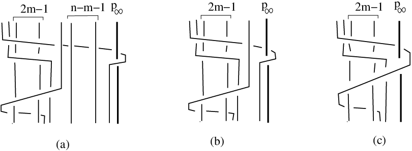
In light of Proposition 3.8, we will consider only where . To prove Theorem 3.11, we first redraw the braid in a conjugate form using induction. Let be the spherical braid drawn in Figure 13. Roughly speaking, conjugation by the braid on is the same as passing a strand counterclockwise around the other strands, and then compensating below after a shift of indices.

Let be the image of in as drawn in Figure 10(b). Let
shown in Figure 14. The inductive step is illustrated in Figure 15. The th braid is constructed from the st braid by conjugating by , for .

The resulting braid takes one of three forms: Figure 16 (a) shows the general case when , Figure 16(b) shows the case when , and Figure 16(c) shows the case when .

Proposition 3.12
When , is a reducible braid.
Proof. By applying one more conjugation by , we obtain the right-hand braid in Figure 17(a). One sees that there is a collection of disjoint disks enclosing pairs of marked points in whose boundaries are left invariant by . The claim now follows from Lemma 2.8.
Proposition 3.13
When , is a periodic braid.
Proof. Figure 17(b) shows an equivalence of spherical braids. It is not hard to see that the right-hand braid is periodic in . The rest follows from Lemma 2.8.
The general case, when , is shown in Figure 18. The transition from Figure 18(a) to 18(b) is given by doing successive conjugations by for .

Now consider the graph map drawn in Figure 19 associated to the preimage of the braid in Figure 18(c) under the contraction map of Lemma 2.8. The unusual numbering comes from the left-to-right ordering of the strands (excluding ) of shown in Figure 3(b) (cf. end of Section 3.3). This ordering proves useful for comparing the transition matrices of and (see Section 3.5).

Proposition 3.14
For , the graph map is a graph map for a conjugate of satisfying (BH:1) and (BH:2).
3.3 Train tracks
In this section, we find train tracks for and , and derive properties of these mapping classes. The train track for associated to is given in Figure 20.

Lemma 3.15
The invariant foliations associated to the pseudo-Anosov representative of have 1-pronged singularities at and marked points, and an - (respectively, -) pronged singularity at the fixed point (respectively, fixed point ).
The train track for associated to is given in Figure 21.

Lemma 3.16
For , the invariant foliations associated to the pseudo-Anosov representative of have 1-pronged singularities at the marked points, an -pronged singularity at the fixed point , and an -pronged singularity at .
Corollary 3.17
For , is pseudo-Anosov, and
A pseudo-Anosov map is said to be orientable if its stable and unstable foliations have only even order prongs.
Proposition 3.18
Let . If both and are odd, there is a pseudo-Anosov element of whose pseudo-Anosov representative is orientable with the same dilatation as .
Proof. Let be the pseudo-Anosov representative of , and let be its lift to the double branched covering of branched along . By Lemma 3.15, is a pseudo-Anosov map on with invariant foliations having two - (respectively, -) pronged singularities above (respectively, ).
Proposition 3.19
There is a pseudo-Anosov element of whose pseudo-Anosov representative is orientable with the same dilatation as , for each with and .
Proof. By Proposition 3.8, we can assume . Since and have the same parity, Lemma 3.16 implies that for the invariant foliations associated to the pseudo-Anosov representative of , the number of prongs (respectively, ) at (respectively ) have opposite parity.
Let be the branched covering of branched along and either if is odd, or if is odd. Let be the lift of to . Then is pseudo-Anosov with dilatation equal that of . Furthermore, by our choice of branch points, the invariant foliations have only even order prongs, and hence are orientable.
We conclude this section by relating the graph maps of and in a way that is compatible with the conjugations used in Section 3.1.

Let be the pseudo-Anosov representative of . Since is a fixed point for , defines a mapping class in . Identify with the graph map on for obtained by pushed forward by the contraction map in Lemma 2.8. Let
be the graph map obtained from after puncturing the sphere at the fixed point for as in Figure 22.

Exchanging the roles of and (i.e., bringing into the visual plane) yields the graph map shown in Figure 23, which is equivalent to . Now remove the marking at and consider the graph map
| (11) |
obtained by a natural identification of edges shown in Figure 23. Figure 24 shows the projection map applied to the image of . The graph map in Figure 19 is the one induced by pushing forward by the map .

3.4 Characteristic equations for dilatation
Consider the graph map , shown in Figure 25. As seen in Figures 12 and 19, the graph maps for and “contain” as the action on a subgraph.

The transition matrix for has the following form with respect to the basis of edges :
The characteristic polynomial for is . As we will see in the proof of Theorem 3.20 given below, the appearance of within the transition matrices of and gives rise to a similar form for their characteristic equations. Given a polynomial of degree , let .
Theorem 3.20
The dilatations of and are as follows:
-
(1) For , the dilatation is the largest root of the polynomial
-
(2) For and , the dilatation is the largest root of the polynomial
Proof. In the discussion at the end of Section 3.3, we saw that, up to isotopy, is a graph map for a pseudo-Anosov representative of , and by Proposition 3.14 is a graph map for a pseudo-Anosov representative of . Thus, to find characteristic polynomials for and , it is enough to compute the transition matrices for and .
Consider the basis for :
The corresponding transition matrix for is given by
We will show that the characteristic polynomial for is given by
The upper left block matrix of corresponding to the vectors is identical to . Multiplying the characteristic polynomials of the upper left and lower right diagonal blocks gives . The rest of the characteristic polynomial has two nonzero summands. One corresponds to the matrix entries marked , and is given by
which yields . The other summand corresponds to the matrix entries marked and is given by
which yields . This completes the proof of (1).
Let be the transition matrix for . We will pull back to an invertible linear transformation on using the map given in (11). Let be the image of under the identification defined by . Then the transition matrix for is the same as except at the vector . As can be seen in Figure 23, we have
Thus, differs from only by changing the entry labeled by both and from to .
Recall that the sign of the entry marked both and in determines the sign of in front of . Since this sign is the only difference between and , the characteristic polynomial for is given by
To finish the proof of (2) we have left to check that is the largest root of . Thus (2) follows if we can show that the extra eigenvalue of has absolute value . We will show below that the extra eigenvalue equals .
From Figure 24, we see that the kernel of the linear map induced by is spanned by
Under the map , we have
and hence, . Thus, the characteristic polynomial for differs from that for by a factor of .
Remark 3.21
Hiroyuki Minakawa independently discovered the pseudo-Anosov maps on constructed in the proof of Proposition 3.19, for the case when , using a beautiful new method for constructing orientable pseudo-Anosov maps on genus surfaces. He also directly computes their dilatation using different techniques from ours.
3.5 Dilatations and Salem-Boyd sequences
In this section, we apply properties of Salem-Boyd sequences to find the least dilatations among and for fixing . We also give bounds on these dilatations.
Given a polynomial of degree , the reciprocal of is . The polynomial satisfying (respectively, ) is a reciprocal polynomial (respectively, anti-reciprocal polynomial). For a monic integer polynomial of degree , the sequence
is called the Salem-Boyd sequence associated to .
Theorem 3.22
Let be a Salem-Boyd sequence associated to . Then is a reciprocal or an anti-reciprocal polynomial, and the set of roots of outside the unit circle converge to those of as goes to infinity.
Theorem 3.22 is a consequence of Rouché’s Theorem applied to the sum
considered as a holomorphic function on the Riemann sphere minus the unit disk.
For a monic integer polynomial , let be the number of roots of outside the unit circle, the maximum norm of roots of , and the product of the norms of roots outside the unit circle, which is called the Mahler measure of .
Corollary 3.23
Let be a Salem-Boyd sequence associated to . Then
-
(1) , and
-
(2) .
Any algebraic integer on the unit circle has a (anti-)reciprocal minimal polynomial. Suppose
where is (anti-)reciprocal and has no roots on the unit circle. Then
We have thus shown the following.
Lemma 3.24
All roots of on the unit circle are also roots of for all .
The following theorem can be proved by first restricting to the case when has no roots on the unit circle, and then by defining a natural deformation of the roots of to those of , which don’t cross the unit circle (see [Boyd2]).
Theorem 3.25
Let be a Salem-Boyd sequence associated to . Then
for all .
We now apply the above results to the Salem-Boyd sequences and of Theorem 3.20. To do this we first study the polynomials .
Lemma 3.26
For all , .
Proof. For we have
and hence has no roots strictly within the unit circle. Therefore, the Mahler measure of must equal the absolute value of the constant coefficient, namely 2.
Corollary 3.27
Fixing and letting increase, the Mahler measures of and converge to 2.
Proof. Apply Corollary 3.23.
Lemma 3.28
The polynomial has one real root outside the unit circle. This root is simple and greater than 1.
Proof. Taking the derivative
we see that is increasing for , and hence also for . Since and , it follows that has a simple root with . Similarly we can show that, for , has no roots for even, and one root if is odd. In the odd case, , so has no real roots strictly less than .
Lemma 3.29
The sequence converges monotonically to 1 from above.
Proof. Since , we know that . Take any . Let be the disk of radius around the origin in the complex plane. Let and . Then for large enough , we have
for all on the boundary of , and and are holomorphic on the complement of in the Riemann sphere. By Rouché’s theorem, , , and hence have the same number of roots outside , which is zero.
To show monotonicity consider . Since satisfies
we have
Since is an increasing function for , we conclude that .
Corollary 3.30
For fixed , the sequences and converge to as sequences in . Furthermore, we can make and arbitrarily small by taking and large enough.
We now determine the monotonicity of and for fixed .
Proposition 3.31
For fixed , the dilatations are strictly monotone decreasing, and for , the dilatations are strictly monotone increasing.
Proof. Consider
Then, for ,
Also . Since , and for , , it follows that and are both negative.
We have
and
which imply that
Since is increasing for , we have and .
Plug into , and subtract :
Since is the largest real root of , we have . We can show that for in a similar way, by adding the formula for to .
Corollary 3.32
We have the inequality
for all with .
We now fix , and show that among the braids and for , has least dilatation.
Proposition 3.33
The braids and satisfy
for , and
for .
Proof. Let . Then plugging into gives
Subtracting
we obtain
Since is the largest real root of , we have . The other inequalities are proved similarly.
Proposition 3.34
For , the dilatations of and satisfy the inequalities
and
with equality if and only if .
Proof. Let . Then
Plugging in the identity
and subtracting this from we have
The roots of are by the quadratic formula. Since
and are both negative, hence . Since is the largest real root of , it follows that .
For the second inequality we plug in into . This gives
Thus, would imply . The polynomial has one real root () and is increasing for . Since is decreasing with and , we see that for . For the remaining case, we check that .
Corollary 3.35
The least dilatation among and for is given by .
By Corollary 3.23, Lemma 3.29 and Proposition 3.31, the dilatations for converge to 1 as approach infinity. We prove the following stronger statement, which implies Theorem 1.1.
Proposition 3.36
The dilatation satisfies
Proof. Using Theorem 3.20, we see that satisfies
| (12) | |||||
Since is the largest real solution, the quadratic formula gives
It follows that
| (13) |
Since for all , (13) implies
We improve the upper bound using an argument conveyed to us by Hiroyuki Minakawa. Rewrite the equation (12) as follows
Factoring out gives
Since , we have
This implies the inequality
for near . Thus, has a real root larger than . Using the quadratic formula again, we see that
and hence
4 Further discussion and questions
As stated in the introduction, the braids with smallest dilatations for 3 and 4 strands are and , respectively. By Proposition 3.33 and Proposition 3.34, for , the minimal dilatations by our construction come from , when ; and , when . For even, there are examples of braids with smaller dilatation than that of , but for odd, we know of no such examples.
For odd, we have , and
Thus, Penner’s lower bound for elements of extend to and we have
For , Zhirov [Zhi] shows that if is pseudo-Anosov with orientable invariant foliations, then is bounded below by the largest root of
For , the braid is pseudo-Anosov, and its lift to a genus surface is orientable. Our formula shows that the dilatation of is the largest root of Zhirov’s equation, and hence achieves the least dilatation of a genus orientable pseudo-Anosov map. This yields the following weaker version of Ham and Song’s result [HS], which doesn’t assume any conditions on the combinatorics of the invariant foliations.
Corollary 4.1
The braid is pseudo-Anosov with smallest dilatation among all braids on strands whose invariant folliations are even-pronged at all interior singularities.
We discuss the following general question and related work on the forcing relation in Section 4.1.
Question 4.2
Is there a pseudo-Anosov braid such that
Let be the subset of mapping classes that arise as the monodromy of a fibered link in , where the fiber has genus and the link has components.
Question 4.3
Is there a strict inequality
In Section 4.2, we briefly discuss what is known about bounds on dilatations of pseudo-Anosov monodromies of fibered links, and show how the braids arise in this class.
4.1 The forcing relation on the braid types
The existence of periodic orbits of dynamical systems can imply the existence of other periodic orbits. Continuous maps of the interval give typical examples for such phenomena [Sha]. In [Boy], Boyland introduces the notion of braid types, and defines a relation on the set of braid types to study an analogous phenomena in the -dimensional case. Let be a set of marked points. There is an isomorphism
Let be an orientation preserving homeomorphism of the disk with a single periodic orbit . The isotopy class of relative to is represented by for some braid . The braid type of for , denoted by is the conjugacy class in the group . To simplify the notation of the braid type, we will write for . Let
and let be the set of all braid types for all homeomorphisms . A relation on is defined as follows: for (),
(For any , .
We say that forces if . It is known that gives a partial order on [Boy], and we call the relation the forcing relation.
The topological entropy gives a measure of orbits complexity for a continuous map of the compact space [Wal]. Let be the topological entropy of . Let be a pseudo-Anosov braid, and let the pseudo-Anosov representative of . Then is equal to , which in turn is the smallest among all with an invariant set such that
(See [FLP].)
From the definition of the forcing relation, we have the following.
Corollary 4.4
If and are pseudo-Anosov, and , then .

The Smale-horseshoe map is a diffeomorphism of the disk such that the action of on three rectangles , and and two half disks is given in Figure 26 [Sma]. The restriction of to () is an affine map such that contracts vertically and stretches horizontally. The restriction of to () is a contraction map. Katok shows that any surface diffeomorphism () with positive topological entropy has a horseshoe in some iterate [Kat], and this suggests that the Smale-horseshoe map is a fundamental model for chaotic dynamics.
The set is invariant under . Let and let
be the shift map. There is a conjugacy between the two maps and as follows:
where
If is a period periodic point, then the finite word is called code for . We say that a braid on the disk is a horseshoe braid if there is a periodic orbit for the Smale-horseshoe map whose braid type is . We define a horseshoe braid type in a similar manner. For the study of the restricted forcing relation on the set of horseshoe braid types, see [Hal],[dCH3],[dCH1], and [dCH2].

The result by Katok together with Corollary 4.4 implies that horseshoe braids are relevant candidates realizing the least dilatation. We note that the braid for each is a horseshoe braid. More precisely, the braid type of the periodic orbit with code or is represented by the conjugate of shown in Figure 18(c). Figure 27 illustrates the periodic orbit with code 10010 and its braid representative. Theorem 15(b) in [dCH2] directly shows the following.
Corollary 4.5
If , then .
By Propositions 3.33 and 3.34, it is natural to ask whether the braid (respectively, ) have the least dilatation among the horseshoe braids on strands (respectively, strands). For the case of even strands, there is a horseshoe braid having dilatation less than . In fact, the braid type of period periodic orbit with code is given by
which satisfies , see [Hal, Table 2].
Question 4.6
For every pseudo-Anosov horseshoe braid , is it true that
4.2 Fibered links
Given a fibered link , with fibering surface , the monodromy
is the map defined up to isotopy such that the complement of a regular neighborhood of in is a mapping torus for . Define to be the characteristic polynomial for the monodromy restricted to first homology . If is a fibered knot, then is the Alexander polynomial of [Rolf], [Kaw].
For a polynomial , let be the maximum norm of roots of (as in Section 3.5). The homological dilatation of a pseudo-Anosov map is defined to be , where is the characteristic polynomial for the restriction of to . Thus, if is a fibered link and is the monodromy, then is the homological dilatation of . The homological and geometric dilatation are equal if has orientable stable and unstable foliations [Ryk]. We will call orientable in this case.
Any monic reciprocal integer polynomial is equal to for some fibered link up to multiples of and [Kan]. In particular, any Perron polynomial can be realized. On the other hand, if the monodromy does not have orientable invariant foliations, then is in general strictly greater than .
For , Leininger [Lei] exhibited a pseudo-Anosov map with dilatation where
A comparison shows that this number is strictly less than our candidate for least element of the braid spectrum , for :
The mapping class is realized as the monodromy of the fibered -pretzel link. Its dilatation is the smallest known Mahler measure among monic integer polynomials [Leh], [Boyd1].
In the rest of this section, we will construct a fibered link whose monodromy is obtained from the braids . Let , and let
Let be the set of marked points on corresponding to the strands of , and let be the double covering of , branched over . Then has one boundary component if is even and two if is odd. Let be the lift of to . Using an argument argument similar to that in the proof of Proposition 2.10, we have
Note that is one-pronged near each of the boundary of if is odd.
Let be the two-bridge link given in Figure 28. By viewing as the result of a sequence of Hopf plumbings (see [Hir, Section 5]) one has the following.

Proposition 4.7
The complement of a regular neighborhood of in is a mapping torus for .
The fibered links and the dilatations of were also studied in [Bri].
Let be the Alexander polynomial for the fibered link . Salem-Boyd sequences for were computed in [Hir]. Proposition 3.18 implies the following.
Lemma 4.8
If and are both odd, then
Question 4.9
Is there a fibered link whose mapping torus is a lift of ?
References
- [BH] M. Bestvina and M. Handel. Train-tracks for suface homeomorphisms. Topology 34 (1994), 1909–140.
- [Bir] J. Birman. Braids, links, and mapping class groups. Number 82 in Annals of Math. Studies. Princeton University Press, Princeton, NJ, 1974.
- [Boyd1] D. W. Boyd. Speculations concerning the range of Mahler’s measure. Canad. Math. Bull. 24 (1981), 453–469.
- [Boyd2] D.W. Boyd. Small Salem numbers. Duke Math. J. 44 (1977), 315–328.
- [Boy] P. Boyland. Relation sets and monotone periodic orbits for annulus homeomorphisms. Comment. Math. Helv. 67 (1992), 203–213.
- [Bri] P. Brinkmann. A Note on pseudo-Anosov maps with small growth rate. Experimental Math. 13 (2004), 49–53.
- [CB] A. Casson and S. Bleiler. Automorphisms of surfaces after Nielsen and Thurston. Cambridge University Press, 1988.
- [dCH1] A. de Carvalho and T. Hall. The forcing relation for horseshoe braid types. Experiment. Math. 11 (2002), 271–288.
- [dCH2] A. de Carvalho and T. Hall. Conjugacies between horseshoe braids. Nonlinearity 16 (4 2003), 1329–1338.
- [dCH3] A. de Carvalho and T. Hall. Braid forcing and star-shaped train tracks. Topology 43 (2004), 247–287.
- [FLP] A. Fathi, F. Laudenbach, and V. Poenaru. Travaux de Thurston sur les surfaces, volume 66-67. Société Mathématique de France, Paris, 1979.
- [Hal] T. Hall. The creation of horseshoes. Nonlinearity 7 (1994), 861–924.
- [HS] J-Y Ham and W. T. Song. The minimum dilatation of pseudo-Anosov 5-braids. preprint (2005).
- [Hir] E. Hironaka. Salem-Boyd sequences and Hopf plumbing. to appear in Osaka J. Math. (2006).
- [Kan] T. Kanenobu. Module d’Alexander des nœuds fibrés et polynôme de Hosokawa des lacements fibrés. Math. Sem. Notes Kobe Univ. 9 (1981), 75–84.
- [Kat] A. Katok. Lyapunov exponents, entropy and periodic orbits for diffeomorphisms. Publ. Math. Inst. Hautes Études Sci. 51 (1980), 137–174.
- [Kaw] A. Kawauchi. A Survey of Knot Theory. Birkhäuser-Verlag, Basel, 1996.
- [KLS] K.H. Ko, J.E. Los, and W.T. Song. Entropies of Braids. J. of Knot Theory and its Ramifications 11 (2002), 647–666.
- [Leh] D. H. Lehmer. Factorization of certain cyclotomic functions. Ann. of Math. 34 (1933), 461–469.
- [Lei] C. Leininger. On groups generated by two positive multi-twists: Teichmuller curves and Lehmer’s number. Geometry & Topology 88 (2004), 1301–1359.
- [Mat] T. Matsuoka. Braids of periodic points and 2-dimensional analogue of Shorkovskii’s ordering. In Ed. G. Ikegami, editor, Dynamical systems and Nonlinear Oscillations, pages 58–72. World Scientific Press, 1986.
- [McM] C. McMullen. Polynomial invariants for fibered 3-manifolds and Teichmüller geodesics for foliataions. Ann. Sci. École Norm. Sup. 33 (2000), 519–560.
- [Pen1] R. Penner. A construction of pseudo-Anosov homeomorphisms. Trans. Amer. Math. Soc. 310 (1988), 179–197.
- [Pen2] R. Penner. Bounds on least dilatations. Proceedings of the A.M.S. 113 (1991), 443–450.
- [PH] R. Penner and J. Harer. Combinatorics of Train Tracks, volume 125 of Ann. of Math. Stud. Princeton University Press, 1991.
- [Rolf] D. Rolfsen. Knots and Links. Publish or Perish, Inc, Berkeley, 1976.
- [Ryk] E. Rykken. Expanding factors for pseudo-Anosov homeomorphisms. Michigan Math. J. 46 (1999), 281–296.
- [Sal] R. Salem. A remarkable class of algebraic integers. Proof of a conjecture of Vijayaraghavan. Duke Math. J. 11 (1944), 103–108.
- [Sha] A. Sharkovskii. Coexistence of cycles of a continuous map of a line into itself. Ukrain. Math. Zh. 16 (1964), 61–71.
- [Sma] S. Smale. Differentiable dynamical systems. Bull. Amer. Math. Soc. 73 (1967), 747–817.
- [Wal] P. Walters. An Introduction to Ergodic Theory. Springer-Verlag, 1982.
- [Zhi] A. Y. Zhirov. On the minimum dilatation of pseudo-Anosov diffeomorphisms on a double torus. Uspekhi Mat. Nauk 50 (1995), 297–198.
Eriko Hironaka
Department of Mathematics
Florida State University
Tallahassee, FL 32306-4510
U.S.A.
Eiko Kin
Department of Mathematics
Faculty of Science
Kyoto University
Kyoto 606-8502
Japan