跳到论文正文
W Papers独立论文阅读器 arXiv:math/0506131 论文正文 计算阅读时间 · 0%
引用这篇论文根据当前论文元数据生成,正式投稿前建议核对。


License: Assumed arXiv.org perpetual non-exclusive license
arXiv:math/0506131v1 [math.CV] 08 Jun 2005

Uniform estimates in the Poincaré-Aronszajn theorem on the separation of singularities of analytic functionsThanks: The first author is partially supported by RFBR grant #03-01-00377 and by the grant for Leading Scientific Schools #NSH-2266-2003.1. The last author is supported by DGICYT grant BFM2002-04072-C02-01 and the CIRIT grant 2001-SGR00172

V.P. Havin Address: St. Petersburg State University. Department of Mathematics and Mechanics, 28 Universitetski pr., St. Petersburg, 198504, Russia Email address: havin@VH1621.spb.edu , A.H. Nersessian Address: Burnside Hall, Department of Mathematics and Statistics McGill University, Montreal H3A 2K6, Canada and J. Ortega-Cerdà Address: Dept. Matemàtica Aplicada i Anàlisi, Universitat de Barcelona, Gran Via 585, 08071 Barcelona, Spain Email address: jortega@ub.edu
Date: August 11, 2026
Abstract.

We study the possibility of splitting any bounded analytic function ff with singularities in a closed set E∪FE\cup F as a sum of two bounded analytic functions with singularities in EE and FF respectively. We obtain some results under geometric restrictions on the sets EE and FF and we provide some examples showing the sharpness of the positive results.

Introduction

Let O⊂ℂO\subset\mathbb{C} be an open set and S1,S2S_{1},S_{2} be two relatively closed subsets in OO, S=S1∪S2S=S_{1}\cup S_{2}. The following result is due to Aronszajn [Aro35]

Theorem 1.

Any function ff analytic in O∖SO\setminus S coincides with (f1+f2)|(O∖S)(f_{1}+f_{2})|_{(O\setminus S)} where fjf_{j} are analytic in O∖SjO\setminus S_{j}, j=1,2j=1,2.

In modern textbooks this fact is treated (if at all) as a trivial example illustrating general sheaf theoretic and ∂¯\bar{\partial} approaches and related to the first Cousin problem; [Aro35] is never quoted (see e.g. [BG91, p. 225], [Hör90]) not to mention its famous predecessors Poincaré [Poi92] and Fréchet [Fre30] although their approaches remain interesting even now. The first version of Theorem 1 with an ingenious proof appeared in 1892 [Poi92] (O=ℂ,S1=[−1,1],S2=(−∞,−1]∪[1,+∞)O=\mathbb{C},\ S_{1}=[-1,1],\ S_{2}=(-\infty,-1]\cup[1,+\infty) which is, of course, equivalent to S1=(−∞,0]S_{1}=(-\infty,0], S2=[0,∞)S_{2}=[0,\infty)). The great author was motivated by his dispute with Borel concerning possible generalizations of the classical notion of analytic continuation. It is not quite clear who was right (see the discussion in [Val54, Chapter IV, section 21-22]), but the explicit (non-linear) construction of f1,f2f_{1},f_{2} given in [Poi92] (exposed also in [Val54]) is very elegant (as was shown in [MH71], in the Poincaré situation there is no linear operator f→(f1,f2)f\to(f_{1},f_{2}) (from H​o​l​(O∖S)→H​o​l​(O∖S1)×H​o​l​(O∖S2)Hol(O\setminus S)\to Hol(O\setminus S_{1})\times Hol(O\setminus S_{2}) where H​o​l​(G)Hol(G) stands for the space of all functions analytic in an open set GG with the usual topology). Various aspects of the separation of singularities in the spirit of the Poincaré-Aronszajn theorem (Theorem 1) are treated in [Val54], [BG91], [Hav58], [Hav84] and [Gau98].

The present article deals with a quantitative aspect of Theorem 1 related to spaces H∞​(G)H^{\infty}(G) of functions bounded and analytic in an open set G⊂ℂG\subset\mathbb{C}. Namely we are interested in the case when ff in Theorem 1 is bounded (i.e. f∈H∞​(O∖S)f\in H^{\infty}(O\setminus S)) and ask whether f1,f2f_{1},f_{2} can be made bounded as well (i.e. fj∈H∞(O∖Sj),j=1,2f_{j}\in H^{\infty}(O\setminus S_{j}),\ j=1,2).

Definition.

Let O,S1,S2,SO,S_{1},S_{2},S be as in Theorem 1. We say (S1,S2)(S_{1},S_{2}) is a bounded separation pair (bs-pair) in OO if any f∈H∞​(O∖S)f\in H^{\infty}(O\setminus S) is representable by the formula

(1) f=f1+f2​ in ​O∖Sf=f_{1}+f_{2}\text{ in }O\setminus S

where fj∈H∞​(O∖Sj)f_{j}\in H^{\infty}(O\setminus S_{j}).

The problem which is implicit in the definition can be restated as follows (just putting Gj=O∖SjG_{j}=O\setminus S_{j}, G=O∖SG=O\setminus S): given open sets G1,G2⊂ℂG_{1},G_{2}\subset\mathbb{C} is it possible to represent an arbitrary f∈H∞​(G)f\in H^{\infty}(G) by (1) with fj∈H∞(Gj),j=1,2f_{j}\in H^{\infty}(G_{j}),\ j=1,2?

We want more or less efficient (preferably geometric) conditions imposed on (S1,S2)(S_{1},S_{2}), resp (G1,G2)(G_{1},G_{2}) and ensuring (1) for any f∈H∞​(O∖S)f\in H^{\infty}(O\setminus S) with fj∈H∞​(O∖Sj)f_{j}\in H^{\infty}(O\setminus S_{j}) (resp. f∈H∞​(G1∩G2),fj∈H∞​(Gj)f\in H^{\infty}(G_{1}\cap G_{2}),\ f_{j}\in H^{\infty}(G_{j})).

One of the first results of this kind is due to Polyakov [Pol83]; it was ancillary in his work on bounded extensions of functions f∈H∞​(C)f\in H^{\infty}(C) to the polydisk 𝔻n\mathbb{D}^{n} (where 𝔻={|z|<1}\mathbb{D}=\{|z|<1\}) for an analytic curve C⊂𝔻nC\subset\mathbb{D}^{n}; see also [HP84]. For G1=𝔻∩{ℑz>0}G_{1}=\mathbb{D}\cap\{\Im z>0\}, G2=𝔻∩{ℜz>0}G_{2}=\mathbb{D}\cap\{\Re z>0\} and any f∈H∞​(G1∩G2)f\in H^{\infty}(G_{1}\cap G_{2}) Polyakov proved (1) in G1∩G2G_{1}\cap G_{2} where fjf_{j} is analytic in GjG_{j} and bounded in Gj∩12​𝔻G_{j}\cap\frac{1}{2}\mathbb{D}.

In [HN01] (whose authors were unaware of [Pol83]) and in [Hav04] the bs-pairs were investigated in a systematic way and in much more general setting. As in [Pol83], in [HN01] it was essential that S1,S2S_{1},S_{2} meet transversally (a generic situation is presented below on Figure 6 (section 3.2 below); the results of [HN01] apply to more general transversal configurations). In [Hav04] a class of tangent bs-pairs was described. Turning to the present article we start with some remarks on bs-pairs.

If S1,S2⊂ℂS_{1},S_{2}\subset\mathbb{C} are compact and disjoint, then (S1,S2)(S_{1},S_{2}) is a bs-pair in ℂ\mathbb{C}: this is an easy consequence of the Cauchy integral formula. Simple examples of pairs which are not bs in ℂ\mathbb{C} (in particular the Poincare pair S1=(−∞,0]S_{1}=(-\infty,0], S2=[0,∞)S_{2}=[0,\infty)) are in [HN01].

The bs-problem is related to the Alice Roth Fusion Lemma (see [Gai87], [Gam69], [Dou66], [HN01]). In particular, the usual localization technique (the Vitushkin operator) gives the following result (see [HN01]): (S1,S2)(S_{1},S_{2}) is a bs-pair in a bounded open set OO if dist⁡(S1,S2)>0\operatorname{dist}(S_{1},S_{2})>0.

Dealing with the bs-problem for a pair (S1,S2)(S_{1},S_{2}) we may always assume that S1∩S2=∅S_{1}\cap S_{2}=\emptyset. (Indeed, (S1,S2)(S_{1},S_{2}) is a bs-pair in OO iff (S1∖S,S2∖s)(S_{1}\setminus S,S_{2}\setminus s) is a bs-pair in O∖sO\setminus s where s=S1∩S2s=S_{1}\cap S_{2}.)

A really subtle and interesting situation arises when S1∩S2=∅S_{1}\cap S_{2}=\emptyset and dist⁡(S1,S2)=0\operatorname{dist}(S_{1},S_{2})=0. Let us denote the closure of a set EE by Clos⁡E\operatorname{Clos}E, and put Kj=Clos⁡SjK_{j}=\operatorname{Clos}S_{j}, j=1,2j=1,2, k=K1∩K2k=K_{1}\cap K_{2}. It is shown in [HN01] that (S1,S2)(S_{1},S_{2}) is a bs-pair in OO iff (S1∩v,S2∩v)(S_{1}\cap v,S_{2}\cap v) is a bs-pair in OO for a neighbourhood vv with respect to ℂ\mathbb{C} of kk. Thus only “the germs of S1S_{1} and S2S_{2} at kk” are responsible for the bs-property of (S1,S2)(S_{1},S_{2}) in OO.

In the present paper (as in [HN01] and [Hav04]) we concentrate on the simplest case when kk is a singleton.

We continue the study of “transversal” pairs (S1,S2)(S_{1},S_{2}) meeting at a point and obtain a very general result applicable to arbitrary relatively closed parts SjS_{j} of the upper half-plane ℂ+\mathbb{C}^{+} separated by two rays η=k​ζ\eta=k\zeta, η=k1​ζ\eta=k_{1}\zeta, ζ>0\zeta>0, 0<arg⁡(k)<arg⁡(k1)<π0<\operatorname{arg}(k)<\operatorname{arg}(k_{1})<\pi. In [HN01] the transversally meeting sets S1S_{1} and S2S_{2} were supposed to be parts of certain rectifiable arcs. We believe, however, that the concrete bounded splittings f→(f1,f2)f\to(f_{1},f_{2}) (f∈H∞​(O∖S),fj∈H∞​(O∖Sj)f\in H^{\infty}(O\setminus S),\ f_{j}\in H^{\infty}(O\setminus S_{j})) constructed in [HN01] are of independent interest; they are also applicable to many tangent pairs (S1,S2)(S_{1},S_{2}), see [Hav04].

Unlike [HN01], we do not exclude the tangency of S1S_{1} and S2S_{2} and find rather sharp descriptions of tangent bs-pairs (S1,S2)(S_{1},S_{2}) in ℂ+\mathbb{C}^{+} when k={0}k=\{0\}; in some cases these descriptions yield necessary and sufficient conditions for a tangent pair of arcs to be bs (Theorem 7).

We mainly put O=ℂ+O=\mathbb{C}^{+}; note that (S1,S2)(S_{1},S_{2}) is a bs-pair in ℂ+\mathbb{C}^{+} iff (ϕ⁡(S1),ϕ⁡(S2))(\phi(S_{1}),\phi(S_{2})) is a bs-pair in ϕ⁡(ℂ+)\phi(\mathbb{C}^{+}) for a conformal homeomorphism ϕ\phi of ℂ+\mathbb{C}^{+}.

The article consists of three paragraphs. In §1 we obtain sufficient conditions for a pair (S1,S2)(S_{1},S_{2}) to be bs in ℂ+\mathbb{C}^{+} (Theorem 4). Our approach is a reduction to the ∂¯\bar{\partial}-problem

(2) ∂¯​u=f​∂¯​χ\bar{\partial}u=f\bar{\partial}\chi

in an open set OO where f∈H∞​(O∖S)f\in H^{\infty}(O\setminus S) is a given function to be split as in (1), and χ\chi is a cutting factor which is ≡1\equiv 1 near S1S_{1} and ≡0\equiv 0 near S2S_{2} in OO; the pair (S1,S2)(S_{1},S_{2}) is bs in OO if (2) has always (for any ff) a bounded solution uu.

Theorems 2 and 3 are preparatory; they are corollaries of deep results by Berndtsson, [Ber92] on bounded solutions of the ∂¯\bar{\partial}-problem in a disc. From them we deduce our main result of §1 (Theorem 4), treating transversal and tangent pairs S1,S2⊂ℂ+S_{1},S_{2}\subset\mathbb{C}^{+} with k={0}k=\{0\}; concrete examples are discussed in 1.4. In 1.5, we give a direct and explicit solution of (2), not using Berndtsson’s results and thus making our §1 essentially self-contained. In 1.6 we give yet another very explicit proof of Theorem 4 for pairs (S1,S2)(S_{1},S_{2}) in ℂ+\mathbb{C}^{+} where S1,S2S_{1},S_{2} are separated by an angle with vertex at the origin. In 1.7 we briefly describe quite explicit bounded splittings f→(f1,f2)f\to(f_{1},f_{2}) applicable to a class of pairs (S1,S2),Sj⊂ℂ+(S_{1},S_{2}),S_{j}\subset\mathbb{C}^{+}; the splittings of 1.5, 1.7 are linear in f∈H∞​(ℂ+∖S)f\in H^{\infty}(\mathbb{C}^{+}\setminus S).

The object of §2 are pairs (S1,S2)(S_{1},S_{2}) of smooth arcs in an angle AA meeting tangentially at its vertex, which are not bs in AA (and, in fact, in any domain O⊃AO\supset A).

The construction is a rather involved “condensation of singularities”, an accumulation of “badly splittable” pairs of arcs in AA based on the Banach theorem on surjective operators. The results are different depending on whether the common tangent of S1S_{1} and S2S_{2} at the vertex is a side of AA (Theorem 6) or is strictly inside AA (Theorem 5). These theorems show the sharpness of the results of §1.

The results of §§1–2 are combined in §3 to state Theorem 7 which includes, among other things, the tangential case when SjS_{j} is the graph of a real 𝒞1+ε\mathcal{C}^{1+\varepsilon}-function ϕj\phi_{j} on [0,b][0,b] such that

ϕj​(0)=ϕj′​(0)=0, 0<ϕ1​(t)<ϕ2​(t)for ​t∈(0,b].\phi_{j}(0)=\phi^{\prime}_{j}(0)=0,\ 0<\phi_{1}(t)<\phi_{2}(t)\quad\text{for }t\in(0,b].

It turns out that (S1,S2)(S_{1},S_{2}) is a bs-pair in ℂ+\mathbb{C}^{+} iff

lim infx→0ϕ2​(x)−ϕ1​(x)ϕ1​(x)>0\liminf_{x\to 0}\frac{\phi_{2}(x)-\phi_{1}(x)}{\phi_{1}(x)}>0

(i.e. S1S_{1} and S2S_{2} are hyperbollicaly separated in ℂ+\mathbb{C}^{+})

In section 3.2 we show that for a Jordan domain G=G1∩G2G=G_{1}\cap G_{2} where the domains GjG_{j} are Jordan as well, a function f∈H∞​(G)f\in H^{\infty}(G) may exist which is not representable as f1+f2f_{1}+f_{2} with fj∈H∞​(Gj)f_{j}\in H^{\infty}(G_{j}). And in section 3.3, we construct an example illustrating the difference between the case of connected sets S1,S2S_{1},S_{2} (arcs) we dealt with in Theorem 7, and disconnected SjS_{j}’s when, apparently, some new results are needed to grasp the bs-property.

1. Some classes of bs-pairs in the upper half-plane

1.1. Reduction to a ∂¯\bar{\partial}-problem

Let S1,S2S_{1},S_{2} be disjoint relatively closed subsets of the domain OO, and f∈H∞​(O∖S)f\in H^{\infty}(O\setminus S), S=S1∪S2S=S_{1}\cup S_{2}. Let U1,U2U_{1},U_{2} be disjoint open neighbourhoods of (resp.) S1,S2S_{1},S_{2} in OO. Consider a locally Lipschitz function χ\chi in OO such that

(3) χ|U1=0,χ|U2=1.\chi|U_{1}=0,\ \chi|U_{2}=1.

Extend ff to OO putting f|S=0f|S=0. Any (distributional) solution uu of the ∂¯\bar{\partial}-problem

(4) ∂¯​u=f​∂¯​χin ​O\bar{\partial}u=f\bar{\partial}\chi\quad\text{in }O

is a continuous function, since f​∂¯​Xf\bar{\partial}X is bounded in OO. We assume u∈𝒞⁡(O)u\in\mathcal{C}(O) and put

f1=fχ−u,f2=f(1−χ)+uin O,f_{1}=f\chi-u,\quad f_{2}=f(1-\chi)+u\quad\text{in }O,

so that f=f1+f2f=f_{1}+f_{2} in OO. Clearly, fjf_{j} is continuous in O∖SjO\setminus S_{j} and ∂¯​fj=0\bar{\partial}f_{j}=0 in O∖SjO\setminus S_{j}, whence it is analytic in O∖SjO\setminus S_{j}. It is bounded if uu is. We arrive at the following conclusion:

if (2) admits a solution u∈L∞​(O)u\in L^{\infty}(O) for any f∈H∞​(O∖S)f\in H^{\infty}(O\setminus S), then (S1,S2)(S_{1},S_{2}) is a bs-pair with respect to OO

1.2. bs-pairs and a result by Berndtsson

Bounded solvability of a general ∂¯\bar{\partial}-equation

(5) ∂¯​u=ρ\bar{\partial}u=\rho

in 𝔻\mathbb{D} was studied in [Ber92]. The result of [Ber92] we need can be easily adapted to ℂ+={ℑz>0}\mathbb{C}^{+}=\{\Im z>0\}. By L1​(E),E⊂ℂL^{1}(E),\ E\subset\mathbb{C}, we mean L1​(E,d​A)L^{1}(E,dA) where d​AdA is the area element.

Theorem 2.

Suppose that ρ∈L1​(ℂ+)\rho\in L^{1}(\mathbb{C}^{+}) vanishes in ℂ+∩{|z|>R}\mathbb{C}^{+}\cap\{|z|>R\} for a positive RR. If

  • (a)

    ρ​d​A\rho\,dA is a Carleson measure in ℂ+\mathbb{C}^{+}, and

  • (b)

    ρ​ℑ⁡z∈L∞​(ℂ+)\rho\Im z\in L^{\infty}(\mathbb{C}^{+}),

then the (distributional) problem (5) has a solution u∈L∞​(ℂ+)u\in L^{\infty}(\mathbb{C}^{+}).

Combining this result with section 1.1 we get

Theorem 3.

Suppose S1,S2⊂ℂ+S_{1},S_{2}\subset\mathbb{C}^{+} are bounded, disjoint, and relatively closed. Suppose there exists a locally Lipschitz real function χ\chi in ℂ+\mathbb{C}^{+} satisfying (3), vanishing in ℂ+∩{|z|>R}\mathbb{C}^{+}\cap\{|z|>R\} and such that

  • (a)

    |∇χ|​d​A|\nabla\chi|\,dA is a Carleson measure in ℂ+\mathbb{C}^{+},

  • (b)

    |∇χ​(ζ)|≤C/ℑ⁡ζ|\nabla\chi(\zeta)|\leq C/\Im\zeta, (ζ∈ℂ+)(\zeta\in\mathbb{C}^{+}).

Then (S1,S2)(S_{1},S_{2}) is a bs-pair in any domain O⊂ℂ+O\subset\mathbb{C}^{+} containing SS.

Proof.

Note that 2​|∂¯​χ|=|∇χ|2|\bar{\partial}\chi|=|\nabla\chi|. By Theorem 2 the ∂¯\bar{\partial}-problem 2 has a bounded solution in ℂ+\mathbb{C}^{+} (thus in OO), and section 1.1 applies. ∎

1.3. Sets S1,S2S_{1},S_{2} separated by graphs

To get a palpable description of some bs-pairs let us assume that there are a number μ>0\mu>0 and a Lipschitz nonnegative function gg on ℝ\mathbb{R} such that

(6) S1⊂U1={ζ+i​η∈ℂ+:η<g⁡(ζ)},S2⊂U2={ζ+i​η∈ℂ+:η>(1+μ)​g​(ζ)}.\begin{split}S_{1}\subset U_{1}&=\{\zeta+i\eta\in\mathbb{C}^{+}:\ \eta<g(\zeta)\},\\ S_{2}\subset U_{2}&=\{\zeta+i\eta\in\mathbb{C}^{+}:\ \eta>(1+\mu)g(\zeta)\}.\end{split}
Theorem 4.

Suppose S1,S2S_{1},S_{2} are relatively closed in ℂ+\mathbb{C}^{+} and bounded. If (6) holds then (S1,S2)(S_{1},S_{2}) satisfies the assumptions of Theorem 3 and thus is a bs-pair in any O⊂ℂ+O\subset\mathbb{C}^{+} containing SS.

Our assumption (6) means that S1,S2S_{1},S_{2} are separated by the corridor {ζ+i​η∈ℂ+:g⁡(ζ)≤η≤(1+μ)​g​(ζ)}\{\zeta+i\eta\in\mathbb{C}^{+}:\ g(\zeta)\leq\eta\leq(1+\mu)g(\zeta)\} whose hyperbolic width is positive (since for g⁡(ζ)>0g(\zeta)>0 the hyperbolic distance between ζ+i​g​(ζ)\zeta+ig(\zeta) and ζ+i⁡(1+μ)​g​(ζ)\zeta+i(1+\mu)g(\zeta) exceeds a positive number not depending on ζ∈ℝ\zeta\in\mathbb{R}). We shall see in §2 that this condition is sharp.

Proof.

Put

χ0​(ξ,η)={0 if ​0<η<g⁡(ξ),η−g⁡(ξ)μ​g​(ξ) if ξ∈ℝ,0<g(ξ)≤η≤(1+μ)g(ξ),1 if ​η>(1+μ)​g​(ξ).\chi_{0}(\xi,\eta)=\begin{cases}0&\text{ if }0<\eta<g(\xi),\\ \frac{\eta-g(\xi)}{\mu g(\xi)}&\text{ if }\xi\in\mathbb{R},0<g(\xi)\leq\eta\leq(1+\mu)g(\xi),\\ 1&\text{ if }\eta>(1+\mu)g(\xi).\end{cases}

Thus χ0​(ξ,η)=1\chi_{0}(\xi,\eta)=1 if ξ∈ℝ\xi\in\mathbb{R}, g⁡(ξ)=0g(\xi)=0, η>0\eta>0. Clearly χ0\chi_{0} is locally Lipschitz on the set {ξ+i​η∈ℂ+:g⁡(ξ)>0}\{\xi+i\eta\in\mathbb{C}^{+}:\ g(\xi)>0\}. If g⁡(ξ)=0g(\xi)=0, η>0\eta>0, then (1+μ)​g​(ξ′)<η′(1+\mu)g(\xi^{\prime})<\eta^{\prime} for ξ′≃ξ\xi^{\prime}\simeq\xi, η′≃η\eta^{\prime}\simeq\eta whence χ0​(ξ′,η′)=1\chi_{0}(\xi^{\prime},\eta^{\prime})=1. We see that χ0≡1\chi_{0}\equiv 1 in a neighbourhood of any point ξ+i​η∈ℂ+\xi+i\eta\in\mathbb{C}^{+} with g⁡(ξ)=0g(\xi)=0, and χ0\chi_{0} is locally Lipschitz in ℂ+\mathbb{C}^{+}. By definition χ0|U1=0\chi_{0}|U_{1}=0, χ0|U2=1\chi_{0}|U_{2}=1. Take a large R>0R>0 (so that S⊂{|ζ|<R}S\subset\{|\zeta|<R\}) and then a 𝒞0∞\mathcal{C}^{\infty}_{0}-function χ1\chi_{1} which is real and ≡1\equiv 1 on {|ζ|<R}\{|\zeta|<R\}. Then

(7) χ=χ0​χ1\chi=\chi_{0}\chi_{1}

satisfies (3). We only have to check (a) and (b) of Theorem 3. But ∇χ=0\nabla\chi=0 on U1∪U2U_{1}\cup U_{2} and

|∇χ​(ξ,η)|≤C⁡(χ1)μ​g​(ξ)​(η​|g′​(ξ)|g⁡(ξ)+1)≤C⁡(g,μ,χ1)/η|\nabla\chi(\xi,\eta)|\leq\frac{C(\chi_{1})}{\mu g(\xi)}\Bigl(\frac{\eta|g^{\prime}(\xi)|}{g(\xi)}+1\Bigr)\leq C(g,\mu,\chi_{1})/\eta

for almost all ξ∈{g>0}\xi\in\{g>0\} and η∈(g⁡(ξ),(1+μ)​g​(ξ))\eta\in(g(\xi),(1+\mu)g(\xi)) (recall that g′∈L∞​(ℝ)g^{\prime}\in L^{\infty}(\mathbb{R})). Thus (b), holds. To prove (a) consider a Carleson box B=(a,b)×(0,b−a)B=(a,b)\times(0,b-a) (a,b∈ℝ,a<ba,b\in\mathbb{R},\ a<b). We have

∫B|∇χ|dA=∫B∩{g(ξ)<η<(1+μ)g(ξ)}|∇χ|dA≤C∫ab(∫g⁡(ξ)(1+μ)​g​(ξ)d​ηηdξ)=Clog(1+μ)(b−a).\int_{B}|\nabla\chi|dA=\int_{B\cap\{g(\xi)<\eta<(1+\mu)g(\xi)\}}|\nabla\chi|dA\leq C\int_{a}^{b}\Bigl(\int_{g(\xi)}^{(1+\mu)g(\xi)}\frac{d\eta}{\eta}d\xi\Bigr)=C\log(1+\mu)(b-a).

∎

1.4. Examples

1.4.1. Example 1

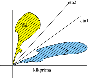
For k>0k>0 put g⁡(ξ)=k​ξg(\xi)=k\xi (ξ≥0\xi\geq 0), g⁡(ξ)=0g(\xi)=0 (ξ<0\xi<0). In this case Theorem 4 is illustrated by pairs (S1,S2)(S_{1},S_{2}) separated by an angle {ξ+iη:ξ>0,kξ<η<(1+μ)kξ}\{\xi+i\eta:\ \xi>0,k\xi<\eta<(1+\mu)k\xi\}.

Refer to caption
Figure 1. Example 1

Compared with [HN01] this result is a progress. In [HN01] some transversally meeting bs-pairs were described with an explicit and elementary splitting formula f=f1+f2f=f_{1}+f_{2} (f∈H∞​(O∖S),fj∈H∞​(O∖Sj)f\in H^{\infty}(O\setminus S),\ f_{j}\in H^{\infty}(O\setminus S_{j})). But in [HN01] certain regularity conditions were imposed on S1,S2S_{1},S_{2} (in particular they had to be contained in a union of rectifiable arcs) whereas Theorem 4 allows arbitrary relatively closed sets separated by an angle.

1.4.2. Example 2
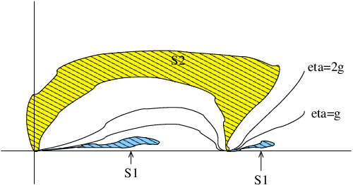
Let G⊂ℝG\subset\mathbb{R} bet a bounded open set. Theorem 4 is applicable to g⁡(ξ)=dist⁡(ξ,ℝ∖G)g(\xi)=\operatorname{dist}(\xi,\mathbb{R}\setminus G) (see figure 2)

Refer to caption
Figure 2. Example2

1.4.3. Example 3

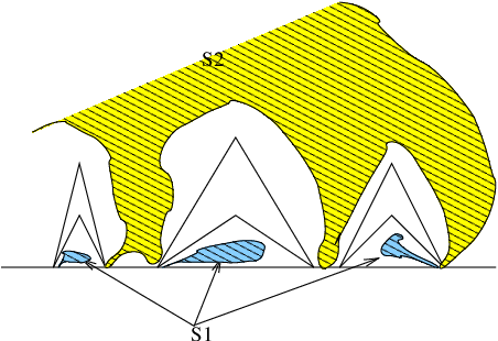
Theorem 4 is also applicable to some tangentially meeting bs-pairs (S1,S2)(S_{1},S_{2}). Suppose g∈𝒞1​(ℝ),g≥0,g⁡(0)=g′​(0)=0g\in\mathcal{C}^{1}(\mathbb{R}),g\geq 0,g(0)=g^{\prime}(0)=0. On figure 3 S1S_{1} and S2S_{2} meet tangentially at the origin, but form a bs-pair in ℂ+\mathbb{C}^{+} (and in any subdomain of ℂ+\mathbb{C}^{+} containing S=S1∪S2S=S_{1}\cup S_{2}).

Refer to caption
Figure 3. Example3

1.5. Theorem 4 revisited: an explicit solution

The ∂¯\bar{\partial}-estimates that we needed included uniform bounds in the whole set ℂ+\mathbb{C}^{+} and not only on the boundary. That is the reason that we could not use Carleson estimates, but had to appeal to the more sophisticated Theorem 4 and we had to assume some extra regularity on the data ρ\rho in (5) apart from the Carleson condition. The estimates by Berndtsson rely on some a priori estimates and therefore the solution is not explicit. Nevertheless Jones has found an explicit non-linear formula [Jon83] to solve the ∂¯\bar{\partial} equation that gives bounded boundary values for the solution when the data is a Carleson measure. Seip has observed (see [Sei04, Chapter1]) that this formula can be adapted to get Theorem 4. For the sake of completeness we present the adapted Jones solution.

Proof.

We assume that |ρ|​d​A|\rho|dA is a Carleson measure in ℂ+\mathbb{C}^{+} and that ρ​ℑ⁡z∈L∞​(ℂ+)\rho\Im z\in L^{\infty}(\mathbb{C}^{+}). Set

u⁡(z)=2​iπ​∫ℑ⁡ζ>01z−ζ​ℑ⁡ζz−ζ¯​exp⁡{α​∫ℑ⁡w≤ℑ⁡ζ(−iz−w¯+iζ−w¯)​|ρ⁡(w)|​𝑑A​(w)}​ρ​(ζ)​𝑑A​(ζ).u(z)=\frac{2i}{\pi}\int_{\Im\zeta>0}\frac{1}{z-\zeta}\frac{\Im\zeta}{z-\bar{\zeta}}\exp\Bigl\{\alpha\int_{\Im w\leq\Im\zeta}\bigl(\frac{-i}{z-\bar{w}}+\frac{i}{\zeta-\bar{w}}\bigr)|\rho(w)|dA(w)\Bigr\}\rho(\zeta)dA(\zeta).

The real number α\alpha can be chosen freely. It is clear that ∂¯​u=ρ\bar{\partial}u=\rho because uu if of the form

u⁡(z)=1π​∫h⁡(z,ζ)z−ζ¯​ρ​(ζ)​𝑑A​(ζ),u(z)=\frac{1}{\pi}\int\frac{h(z,\zeta)}{z-\bar{\zeta}}\rho(\zeta)dA(\zeta),

and for any ζ\zeta, h⁡(⋅,ζ)h(\cdot,\zeta) is holomorphic and in the diagonal h⁡(z,z)=1h(z,z)=1. The hard part is to obtain estimates for uu. We take

α−1=supℑ⁡ζ>0∫ℑ⁡w≤ℑ⁡ζ2​ℑ⁡ζ|w−ζ¯|2​|ρ⁡(w)|​𝑑A​(w).\alpha^{-1}=\sup_{\Im\zeta>0}\int_{\Im w\leq\Im\zeta}\frac{2\Im\zeta}{|w-\bar{\zeta}|^{2}}|\rho(w)|dA(w).

This supremum is finite because we assume that |ρ|​d​A|\rho|dA is a Carleson measure. We get

|u⁡(z)|≤2π​α​∫ℑ⁡ζ>0α|z−ζ|​ℑ⁡ζ|z−ζ¯|​exp⁡{α​∫ℑ⁡w≤ℑ⁡ζ−(ℑ⁡w+ℑ⁡z)|z−w¯|2+2​ℑ⁡ζ|ζ−w¯|2​|ρ⁡(w)|​dA​(w)}​|ρ⁡(ζ)|​dA​(ζ).\begin{split}&|u(z)|\leq\\ &\frac{2}{\pi\alpha}\int_{\Im\zeta>0}\!\frac{\alpha}{|z-\zeta|}\frac{\Im\zeta}{|z-\bar{\zeta}|}\exp{\Bigl\{\alpha\int_{\Im w\leq\Im\zeta}\frac{-(\Im w+\Im z)}{|z-\bar{w}|^{2}}+\frac{2\Im\zeta}{|\zeta-\bar{w}|^{2}}|\rho(w)|dA(w)\Bigr\}|\rho(\zeta)|dA(\zeta)}.\end{split}

We use the definition of α\alpha and we get

|u⁡(z)|≤2​eπ​α​∫ℑ⁡ζ>0α|z−ζ|​ℑ⁡ζ|z−ζ¯|​exp⁡{α​∫ℑ⁡w≤ℑ⁡ζ−(ℑ⁡(w)+ℑ⁡(z))|z−w¯|2​|ρ⁡(w)|​𝑑A​(w)}​|ρ⁡(ζ)|​𝑑A​(ζ).|u(z)|\leq\frac{2e}{\pi\alpha}\int_{\Im\zeta>0}\!\frac{\alpha}{|z-\zeta|}\frac{\Im\zeta}{|z-\bar{\zeta}|}\exp{\Bigl\{\alpha\int_{\Im w\leq\Im\zeta}\frac{-(\Im(w)+\Im(z))}{|z-\bar{w}|^{2}}|\rho(w)|dA(w)\Bigr\}|\rho(\zeta)|dA(\zeta)}.

We then write

|u⁡(z)|≤I1+I2,|u(z)|\leq I_{1}+I_{2},

where

I1=2​eα​π​∫2​|z−ζ|≥ℑ⁡zα|z−ζ|​ℑ⁡ζ|z−ζ¯|​exp⁡{α​∫ℑ⁡w≤ℑ⁡ζ−(ℑ⁡(w)+ℑ⁡(z))|z−w¯|2​|ρ⁡(w)|​𝑑A​(w)}​|ρ⁡(ζ)|​𝑑A​(ζ)I_{1}=\frac{2e}{\alpha\pi}\int_{2|z-\zeta|\geq\Im z}\frac{\alpha}{|z-\zeta|}\frac{\Im\zeta}{|z-\bar{\zeta}|}\exp{\Bigl\{\alpha\int_{\Im w\leq\Im\zeta}\frac{-(\Im(w)+\Im(z))}{|z-\bar{w}|^{2}}|\rho(w)|dA(w)\Bigr\}|\rho(\zeta)|dA(\zeta)}

and

I2=2​eα​π​∫2​|z−ζ|<ℑ⁡zα|z−ζ|​ℑ⁡ζ|z−ζ¯|​exp⁡{α​∫ℑ⁡w≤ℑ⁡ζ−(ℑ⁡(w)+ℑ⁡(z))|z−w¯|2​|ρ⁡(w)|​𝑑A​(w)}​|ρ⁡(ζ)|​𝑑A​(ζ).I_{2}=\frac{2e}{\alpha\pi}\int_{2|z-\zeta|<\Im z}\!\frac{\alpha}{|z-\zeta|}\frac{\Im\zeta}{|z-\bar{\zeta}|}\exp{\Bigl\{\alpha\int_{\Im w\leq\Im\zeta}\frac{-(\Im(w)+\Im(z))}{|z-\bar{w}|^{2}}|\rho(w)|dA(w)\Bigr\}|\rho(\zeta)|dA(\zeta)}.

When 2​|z−ζ|≥ℑ⁡z2|z-\zeta|\geq\Im z, then |z−ζ|≥|z−ζ¯|/5|z-\zeta|\geq|z-\bar{\zeta}|/5 and thus I1I_{1} is bounded by a constant times

(8) 1α​∫ℑ⁡ζ>0α​ℑ⁡ζ|z−ζ¯|2​exp⁡{α​∫ℑ⁡w≤ℑ⁡ζ−ℑ⁡(w)|z−w¯|2​|ρ⁡(w)|​𝑑A​(w)}​|ρ⁡(ζ)|​𝑑A​(ζ).\frac{1}{\alpha}\int_{\Im\zeta>0}\frac{\alpha\Im\zeta}{|z-\bar{\zeta}|^{2}}\exp{\Bigl\{\alpha\int_{\Im w\leq\Im\zeta}\frac{-\Im(w)}{|z-\bar{w}|^{2}}|\rho(w)|dA(w)\Bigr\}|\rho(\zeta)|dA(\zeta)}.

If ff is any positive function defined on t≥0t\geq 0 and R0=∫0∞f⁡(t)​𝑑tR_{0}=\int_{0}^{\infty}f(t)dt (which may eventually be ∞\infty), then

∫0∞f(r)exp(−∫0rf(t)dt)dr=∫0R0e−tdt≤1.\int_{0}^{\infty}f(r)\exp\Bigl(-\int_{0}^{r}f(t)\,dt\Bigr)\,dr=\int_{0}^{R_{0}}e^{-t}\,dt\leq 1.

We apply this inequality to the function

f⁡(t)=∫ℝα​t|z−(x−i​t)|2​|ρ⁡(x+i​t)|​𝑑x,f(t)=\int_{\mathbb{R}}\frac{\alpha t}{|z-(x-it)|^{2}}|\rho(x+it)|\,dx,

and we get that (8) is bounded by α−1\alpha^{-1}.

On the other hand I2I_{2} is easy to estimate if we drop the exponential term and use the fact that |ρ⁡(z)|≤C/ℑ⁡z|\rho(z)|\leq C/\Im z. ∎

1.6. An explicit solution of (2) for transversally meeting sets S1,S2⊂ℂ+S_{1},S_{2}\subset\mathbb{C}^{+}

Here we return to Example 1 of section 1.4 and give another very simple solution of the problem

(9) ∂¯​u=ρ,ρ=f​∂¯​χ,\bar{\partial}u=\rho,\ \rho=f\bar{\partial}\chi,

where χ\chi (see (7)) corresponds to gg which is zero on (−∞,0](-\infty,0] and is linear on [0,∞)[0,\infty): g⁡(ξ)=k​ξg(\xi)=k\xi, ξ≥0\xi\geq 0, for a k>0k>0. The sets S1,S2S_{1},S_{2} are separated by the angle

Ak,μ={(ξ,η):k​ξ<η<(1+μ)​k​ξ},A_{k,\mu}=\{(\xi,\eta):k\xi<\eta<(1+\mu)k\xi\},

and ∂χ\partial\chi is supported by a sector T=Ak,μ∩{|z|<R}T=A_{k,\mu}\cap\{|z|<R\}. Put u=Cρ−au=C^{\rho}-a, where Cρ=1π​ρ⋆1zC^{\rho}=\frac{1}{\pi}\rho\star\frac{1}{z} is the standard solution of (9) and

a⁡(ζ)=1π​∫ℂ+z¯z​ρ⁡(z)ζ−z¯​𝑑A​(z),ζ∈ℂ+.a(\zeta)=\frac{1}{\pi}\int_{\mathbb{C}^{+}}\frac{\bar{z}}{z}\frac{\rho(z)}{\zeta-\bar{z}}dA(z),\qquad\zeta\in\mathbb{C}^{+}.

Note that ρ≡0\rho\equiv 0 off TT, and |ρ⁡(z)|≤C/ℑ⁡z≃1/|z||\rho(z)|\leq C/\Im z\simeq 1/|z| for z∈Tz\in T whence ρ∈L1​(ℂ+,d​A)\rho\in L^{1}(\mathbb{C}^{+},dA), and functions Cρ,aC^{\rho},a make sense.

Clearly, ∂¯​u=ρ\bar{\partial}u=\rho, since aa is analytic in ℂ+\mathbb{C}^{+}, and we only have to prove that uu is bounded in ℂ+\mathbb{C}^{+}. We have

u⁡(ζ)=2​i​ζπ​∫Tℑ⁡z​∂¯​χ​(z)​f​(z)​d​A​(z)z​(ζ−z)​(ζ−z¯),u(\zeta)=\frac{2i\zeta}{\pi}\int_{T}\frac{\Im z\bar{\partial}\chi(z)f(z)dA(z)}{z(\zeta-z)(\zeta-\bar{z})},

whence

(10) |u⁡(ζ)|≤c​|ζ|​∫Td​A​(z)|z|​|ζ−z|​|ζ−z¯|=C​|ζ|​J​(ζ),ζ∈ℂ+.|u(\zeta)|\leq c|\zeta|\int_{T}\frac{dA(z)}{|z||\zeta-z||\zeta-\bar{z}|}=C|\zeta|J(\zeta),\quad\zeta\in\mathbb{C}^{+}.

Fix a small q>0q>0 (to be specified later). Then

J(ζ)≤∫T∩{|z−ζ|<q|ζ|}+∫T∩{|z−ζ|>q​|ζ|,|z|>q​|ζ|}+∫T∩{|z−ζ|>q​|ζ|,|z|<q​|ζ|}=I+II+III,J(\zeta)\leq\int_{T\cap\{|z-\zeta|<q|\zeta|\}}+\int_{T\cap\{|z-\zeta|>q|\zeta|,\ |z|>q|\zeta|\}}+\int_{T\cap\{|z-\zeta|>q|\zeta|,\ |z|<q|\zeta|\}}=I+II+III,

Now, |z|≃ℑ⁡z|z|\simeq\Im z for z∈Tz\in T. Estimating I we may write |z|≥|ζ|−|z−ζ|≥(1−q)​|ζ||z|\geq|\zeta|-|z-\zeta|\geq(1-q)|\zeta|,

|z¯−ζ|≥2​ℑ⁡z−|z−ζ|≥c​|z|−q|ζ|≥c′​|ζ||\bar{z}-\zeta|\geq 2\Im z-|z-\zeta|\geq c|z|-q|\zeta|\geq c^{\prime}|\zeta|

where c=c⁡(k,μ)>0c=c(k,\mu)>0, c′=c⁡(1−q)−q>0c^{\prime}=c(1-q)-q>0 if qq is small, and

(11) I≤c1|ζ|2​∫|z−ζ|<q​|ζ|d​A​(z)|ζ−z|=c2|ζ|.I\leq\frac{c_{1}}{|\zeta|^{2}}\int_{|z-\zeta|<q|\zeta|}\frac{dA(z)}{|\zeta-z|}=\frac{c_{2}}{|\zeta|}.

The Hölder inequality (with p=3p=3, q=3/2q=3/2) and |z¯−ζ|≥|z−ζ||\bar{z}-\zeta|\geq|z-\zeta| give

(12) I​I≤∫|z−ζ|>q​|ζ|,|z|>q​|ζ|d​A​(z)|z|​|z−ζ|2≤(∫|z|>q​|ζ|d​A​(z)|z|3)1/3​(∫|z−ζ|>q​|ζ|d​A​(z)|z−ζ|3)2/3=c3|ζ|.II\leq\int_{|z-\zeta|>q|\zeta|,\ |z|>q|\zeta|}\frac{dA(z)}{|z||z-\zeta|^{2}}\leq\left(\int_{|z|>q|\zeta|}\frac{dA(z)}{|z|^{3}}\right)^{1/3}\left(\int_{|z-\zeta|>q|\zeta|}\frac{dA(z)}{|z-\zeta|^{3}}\right)^{2/3}=\frac{c_{3}}{|\zeta|}.

At last,

(13) I​I​I≤∫|z−ζ|>q​|ζ|,|z|<q​|ζ|d​A​(z)|z|​|z−ζ|2≤1q2​|ζ|2​∫|z|<q⁡(|ζ|CLOSEd​A​(z)|z|=c4|ζ|.III\leq\int_{|z-\zeta|>q|\zeta|,\ |z|<q|\zeta|}\frac{dA(z)}{|z||z-\zeta|^{2}}\leq\frac{1}{q^{2}|\zeta|^{2}}\int_{|z|<q(|\zeta|}\frac{dA(z)}{|z|}=\frac{c_{4}}{|\zeta|}.

Combining (10) with (11)–(13) we see that uu is bounded. ∎

1.7. Another explicit and bounded solution to equation (2)

Here we again exploit the special form of the right side of (2) (recall that Theorem 3 is aimed at general right sides ρ∈L1​(ℂ+)\rho\in L^{1}(\mathbb{C}^{+}), but we only deal with ρ=f​∂¯​χ\rho=f\bar{\partial}\chi, where f∈H∞​(ℂ+∖S)f\in H^{\infty}(\mathbb{C}^{+}\setminus S) and χ\chi is a smooth cutting factor).

This time we consider a function g:ℝ→[0,+∞)g:\mathbb{R}\to[0,+\infty) and assume g∈𝒞1+ε​(ℝ)g\in\mathcal{C}^{1+\varepsilon}(\mathbb{R}), ε>0\varepsilon>0, g≡0g\equiv 0 on (−∞,0](-\infty,0], g⁡(x)>0g(x)>0 for x>0x>0 (in Theorem 4 gg was a Lipschitz function and it could vanish at some positive points). The functions χ0,χ1,χ\chi_{0},\ \chi_{1},\ \chi are the same as in Theorem 4. Fix a small b>0b>0 so that χ1≡1\chi_{1}\equiv 1 on the corridor

Gb={ξ+iη: 0<ξ<b,g(ξ)<η<(1+μ)g(ξ)},G_{b}=\{\xi+i\eta:\ 0<\xi<b,\ g(\xi)<\eta<(1+\mu)g(\xi)\},

and χ0≡χ\chi_{0}\equiv\chi on GbG_{b}. For t∈[1,1+μ]t\in[1,1+\mu] put γt​(ξ)=ξ+i​t​g​(ξ)\gamma_{t}(\xi)=\xi+itg(\xi), 0≤ξ≤b0\leq\xi\leq b.

Suppose ff is as in Theorem 4 (f∈L∞​(ℂ+)f\in L^{\infty}(\mathbb{C}^{+}), f|S=0f|S=0, ff is analytic in ℂ+∖S\mathbb{C}^{+}\setminus S). Put

u⁡(ζ)=1π​∫ℂ+f⁡(z)​∂¯​χ​(z)ζ−z​𝑑A​(z)+μ2​π​i​∫γ¯1f⁡(z¯)​d​zζ−z,ζ∈ℂ+.u(\zeta)=\frac{1}{\pi}\int_{\mathbb{C}^{+}}\frac{f(z)\bar{\partial}\chi(z)}{\zeta-z}dA(z)+\frac{\mu}{2\pi i}\int_{\bar{\gamma}_{1}}\frac{f(\bar{z})dz}{\zeta-z},\ \zeta\in\mathbb{C}^{+}.

Then uu is bounded in ℂ+\mathbb{C}^{+} and satisfies (2).

Recall that γ1\gamma_{1} is the path t→t+i​g​(t)t\to t+ig(t), t∈[0,b]t\in[0,b], so that the path γ¯1\bar{\gamma}_{1} (i.e. the reflected graph of gg) does not intersect ℂ+\mathbb{C}^{+}, and the contour integral is analytic in ℂ+\mathbb{C}^{+}. At the same time the double integral represents “the standard solution of (2)” (note that ∂¯​χ\bar{\partial}\chi is summable in GbG_{b}, see the last estimate in Section 1.3). Thus our uu staisfies (2) in ℂ+\mathbb{C}^{+}, and the only problem is its boundedness. The standard solution may blow up at the origin, but its growth is counterbalanced by the contour integral. A detailed proof will be given in [HO05].

Our definition of uu combined with Section 1.1 generates a linear operator f→(f1,f2)f\to(f_{1},f_{2}) splitting f∈H∞​(ℂ+∖S)f\in H^{\infty}(\mathbb{C}^{+}\setminus S) into the sum of functions fj∈H∞​(ℂ+∖Sj)f_{j}\in H^{\infty}(\mathbb{C}^{+}\setminus S_{j}), j=1,2j=1,2.

2. Negative results

In this paragraph we describe some pairs (S1,S2)(S_{1},S_{2}) of subsets of an angle AA which are not bs-pairs in AA (Theorems 5, 6 in section 2.5.3 and 2.6). Combined with the results of §1 they give some necessary and sufficient geometric conditions for two smooth graphs to form a bs-pair in ℂ+\mathbb{C}^{+} (see §3). We start with preliminary technical results on “badly splittable” pairs of arcs K1,K2K_{1},K_{2} in a domain OO which means the existence of ϕ∈H∞​(O∖K)\phi\in H^{\infty}(O\setminus K), K=K1∪K2K=K_{1}\cup K_{2} with |ϕ|≤1|\phi|\leq 1 in O∖KO\setminus K and such that a representation ϕ=ϕ1+ϕ2\phi=\phi_{1}+\phi_{2}, ϕj∈H∞​(O∖K)\phi_{j}\in H^{\infty}(O\setminus K), is only possible with a very big sup{|ϕ1​(ζ)|:ζ∈O∖K1}\sup\{|\phi_{1}(\zeta)|:\ \zeta\in O\setminus K_{1}\}. If S1,S2⊂OS_{1},S_{2}\subset O contain the elements K1,K2K_{1},K_{2} of arbitrarily badly splittable pairs (K1,K2)(K_{1},K_{2}) (i.e. Sj⊃KjS_{j}\supset K_{j}, j=1,2j=1,2), then (S1,S2)(S_{1},S_{2}) is not a bs-pair in OO. These vague considerations are made precise in sections 2.1–2.4, and then applied to quite concrete Theorems 5, 6.

2.1. Cells and their rotundities

A cell is by definition a pair (g,A)(g,A) where gg is a Jordan domain with a rectifiable boundary ∂g\partial g, and AA, “the center” of gg, is a point in gg. Sometimes we write gg instead of (g,A)(g,A). Put

ρ⁡(g)(=ρ⁡((g,A)))=2​π​dist⁡(A,∂g)l⁡(∂g)\rho(g)(=\rho((g,A)))=\frac{2\pi\operatorname{dist}(A,\partial g)}{l(\partial g)}

where l⁡(∂g)l(\partial g) denotes the length of ∂g\partial g. Clearly, ρ⁡(g)≤1\rho(g)\leq 1, a geometrically obvious fact (an instant proof is given by the formula 1=(2​π​i)−1​∫∂gd​zz−A1=(2\pi i)^{-1}\int_{\partial g}\frac{dz}{z-A}); the equality ρ⁡(g)=1\rho(g)=1 occurs iff gg is a disc centered at AA. We call ρ⁡(g)\rho(g) the rotundity of the cell g(=(g,A))g(=(g,A)).

2.2. Functions at a large distance from H∞​(g)H^{\infty}(g) in a cell gg

Let KK be a compact subset of gg containing AA. We assume AA to be a boundary point of KK (in our applications KK will be just a simple arc)

Lemma 1.

Let ϕ\phi be a function analytic in ℂ∖K\mathbb{C}\setminus K, ϕ⁡(∞)=0\phi(\infty)=0. Then any h∈H∞​(g)h\in H^{\infty}(g) satisfies

(14) ‖ϕ−h‖g∖K≥ρ⁡(g)2​lim supA|ϕ|,\|\phi-h\|_{g\setminus K}\geq\frac{\rho(g)}{2}\limsup_{A}|\phi|,

where ∥⋅∥E\|\cdot\|_{E} denotes ∥⋅∥∞,E\|\cdot\|_{\infty,E}.

In other words, if ϕ\phi is very big near AA and (g,A)(g,A) is sufficiently rotund, then any h∈H∞​(g)h\in H^{\infty}(g) is far away from ϕ\phi in H∞​(g∖K)H^{\infty}(g\setminus K).

Proof.

Any h∈H∞​(g)h\in H^{\infty}(g) has the angular boundary value h⁡(g)h(g) at almost every q∈∂gq\in\partial g, and

h⁡(p)≡12​π​i​∮∂gh⁡(q)q−p​𝑑qfor ​p∈g.h(p)\equiv\frac{1}{2\pi i}\oint_{\partial g}\frac{h(q)}{q-p}\,dq\qquad\text{for }p\in g.

Moreover, ∮∂gϕ⁡(q)q−p≡0\oint_{\partial g}\frac{\phi(q)}{q-p}\equiv 0 for p∈gp\in g. Thus putting ∥⋅∥=∥⋅∥g∖K\|\cdot\|=\|\cdot\|_{g\setminus K}, we have

|ϕ⁡(p)|≤|h⁡(p)|+‖ϕ−h‖=12​π​|∮∂gh⁡(q)−ϕ⁡(q)q−p​dq|+‖ϕ−h‖≤(1ρ⁡(g)+1)​‖ϕ−h‖≤2ρ⁡(g)​‖ϕ−h‖.\begin{split}|\phi(p)|\leq|h(p)|+\|\phi-h\|=\\ \frac{1}{2\pi}\Bigl|\oint_{\partial g}\frac{h(q)-\phi(q)}{q-p}dq\Bigr|+\|\phi-h\|\leq\\ \bigl(\frac{1}{\rho(g)}+1\bigr)\|\phi-h\|\leq\frac{2}{\rho(g)}\|\phi-h\|.\end{split}

Letting p→Ap\to A we get (14). ∎

2.3. Pairs not admitting bounded separation in a domain (an abstract scheme)

Lemma 1 suggests a method to construct pairs (S1,S2)(S_{1},S_{2}) which are not bs in a domain OO.

2.3.1.

Suppose S1,S2S_{1},S_{2} are relatively closed disjoint and nowhere dense parts of a domain OO. Suppose there is a number CC such that for any (big) M>0M>0 there exists a cell g(=(g,A))g\bigl(=(g,A)\bigr), g⊂Og\subset O, and a pair (K1,K2)(K_{1},K_{2}) of compacts such that Kj⊂SjK_{j}\subset S_{j}, j=1,2j=1,2, and K1⊂gK_{1}\subset g, ρ⁡(g)≥C−1\rho(g)\geq C^{-1}, and for a pair (ϕ1,ϕ2)(\phi_{1},\phi_{2}) of functions analytic, respectively, in ℂ∖Kj\mathbb{C}\setminus K_{j}, j=1,2j=1,2, we have

ϕ1​(∞)=ϕ2​(∞)=0,|ϕ1+ϕ2|≤C​ in ​ℂ∖K,K=K1∪K2,\phi_{1}(\infty)=\phi_{2}(\infty)=0,\ |\phi_{1}+\phi_{2}|\leq C\text{ in }\mathbb{C}\setminus K,\ K=K_{1}\cup K_{2},

whereas

(15) lim supA|ϕ1|>M.\limsup_{A}|\phi_{1}|>M.
Lemma 2.

If S1,S2S_{1},S_{2} and OO enjoy property  2.3.1, then (S1,S2)(S_{1},S_{2}) is not a bs-pair in OO.

Note that ϕj∈H∞​(ℂ∖Kj)\phi_{j}\in H^{\infty}(\mathbb{C}\setminus K_{j}), j=1,2j=1,2, since K1,K2K_{1},K_{2} are disjoint.

Proof.

Put S=S1∪S2S=S_{1}\cup S_{2}. If (S1,S2)(S_{1},S_{2}) were a bs-pair in OO, then the operator (f1,f2)→(f1+f2)​(O∖S)(f_{1},f_{2})\to(f_{1}+f_{2})(O\setminus S) from OPENH∞​(O∖S1)×H∞​(O∖S2))H^{\infty}(O\setminus S_{1})\times H^{\infty}(O\setminus S_{2})) to H∞​(O∖S)H^{\infty}(O\setminus S) would be surjective, and, by the Banach theorem, we could find a number N>0N>0 such that any f∈H∞​(O∖S)f\in H^{\infty}(O\setminus S) would admit a splitting

(16) f=f1+f2in ​O∖S,f=f_{1}+f_{2}\qquad\text{in }O\setminus S,

with fj∈H∞​(O∖Sj)f_{j}\in H^{\infty}(O\setminus S_{j}), ‖fj‖O∖Sj≤N​‖f‖O∖S\|f_{j}\|_{O\setminus S_{j}}\leq N\|f\|_{O\setminus S}.

But 2.3.1 forbids the existence of such number NN. Indeed, let Kj​ϕjK_{j}\ \phi_{j} be as in 2.3.1 where a big M=M⁡(N)M=M(N) will be specified later. Put fj0=ϕj|(O∖Kj)f_{j}^{0}=\phi_{j}|(O\setminus K_{j}), j=1,2j=1,2, and f=f10+f20f=f_{1}^{0}+f_{2}^{0} in O∖KO\setminus K, K=K1∪K2K=K_{1}\cup K_{2}. Then for any representation (16) of ff we get

f1=f10−h​ in ​O∖S1f2=f20+h​ in ​O∖S2\begin{split}f_{1}&=f_{1}^{0}-h\text{ in }O\setminus S_{1}\\ f_{2}&=f_{2}^{0}+h\text{ in }O\setminus S_{2}\end{split}

where h∈H∞​(O)h\in H^{\infty}(O), since f10−f1f_{1}^{0}-f_{1} and f20−f2f_{2}^{0}-f_{2} are mutual analytic continuations from O∖SO\setminus S across S2S_{2} and S1S_{1}. But f1f_{1} is in fact defined and analytic not only on O∖S1O\setminus S_{1}, but in O∖K1O\setminus K_{1}, since f10∈H∞​(O∖K1)f_{1}^{0}\in H^{\infty}(O\setminus K_{1}), h∈H∞​(O)h\in H^{\infty}(O). Moreover, ‖f1‖O∖K1=‖f1‖O∖S1\|f_{1}\|_{O\setminus K_{1}}=\|f_{1}\|_{O\setminus S_{1}}, since S1S_{1} has no interior points. Now since h∈H∞​(g)h\in H^{\infty}(g) and ρ⁡(g)≥C−1\rho(g)\geq C^{-1}, by Lemma 1 and (15) we have

‖f1‖O∖S1=‖f1‖O∖K1≥M2​C.\|f_{1}\|_{O\setminus S_{1}}=\|f_{1}\|_{O\setminus K_{1}}\geq\frac{M}{2C}.

For an arbitrary N>0N>0 take M>2​N​C2M>2NC^{2}. We get a contradiction: given N>0N>0, no splitting (16) of ff with fj∈H∞​(O∖Sj)f_{j}\in H^{\infty}(O\setminus S_{j}) satisfies ‖f1‖O∖S1≤N​‖f‖O∖S\|f_{1}\|_{O\setminus S_{1}}\leq N\|f\|_{O\setminus S} (recall that ‖f‖O∖S≤C\|f\|_{O\setminus S}\leq C). ∎

2.3.2.

Now we are ready to describe a general scheme of constructing triples (O,S1,S2)(O,S_{1},S_{2}) where OO is a domain, SjS_{j} its relatively closed and disjoint subsets such that (S1,S2)(S_{1},S_{2}) is not a bs-pair in OO. Namely, suppose we have constructed two families (K1x)x∈E(K_{1}^{x})_{x\in E}, (K2x)x∈E(K_{2}^{x})_{x\in E} of compact simple arcs and two families (ϕ1x)x∈E(\phi_{1}^{x})_{x\in E}, (ϕ2x)x∈E(\phi_{2}^{x})_{x\in E} of functions in, respectively, H∞​(ℂ∖Kjx)H^{\infty}(\mathbb{C}\setminus K_{j}^{x}), j=1,2j=1,2, and a family of points (Ax)x∈E(A^{x})_{x\in E} such that

  • (a)

    K1x∩K2x=∅K_{1}^{x}\cap K_{2}^{x}=\emptyset;

  • (b)

    ϕjx(∞)=0,j=1,2\phi_{j}^{x}(\infty)=0,\ j=1,2;

  • (c)

    supx∈E‖ϕ1x+ϕ2x‖ℂ∖Kx<+∞\sup_{x\in E}\|\phi^{x}_{1}+\phi_{2}^{x}\|_{\mathbb{C}\setminus K^{x}}<+\infty, Kx:=K1x∪K2xK^{x}:=K_{1}^{x}\cup K_{2}^{x};

  • (d)

    Ax∈K1xA^{x}\in K_{1}^{x} and supx∈Elim supAx|ϕ1x|=+∞\sup_{x\in E}\limsup_{A^{x}}|\phi_{1}^{x}|=+\infty.

The last element of our construction is a family (gx,Ax)x∈E(g^{x},A^{x})_{x\in E} of cells such that

  • (e)

    K1x⊂gxK_{1}^{x}\subset g^{x}, x∈Ex\in E, and gxg^{x} are uniformly rotund (i.e. infx∈Eρ⁡(gx)>0\inf_{x\in E}\rho(g^{x})>0).

Any family of quintuples (K1x,K2x,ϕ1x,ϕ2x,gx)(K_{1}^{x},K_{2}^{x},\phi_{1}^{x},\phi_{2}^{x},g^{x}) enjoying (a)–(e) generates plenty of “bad” triples (O,S1,S2)(O,S_{1},S_{2}). Indeed, for any domain OO containing ∪x∈E(gx∪K2x)\cup_{x\in E}(g^{x}\cup K_{2}^{x}), any pair (S1,S2)(S_{1},S_{2}) of its disjoint relatively closed and nowhere dense subsets is not a bs-pair with respect to OO provided

S1⊃∪x∈EKx1,S2⊃∪x∈EKx2.S_{1}\supset\cup_{x\in E}K^{x}_{1},\qquad S_{2}\supset\cup_{x\in E}K^{x}_{2}.

This is an immediate consequence of Lemma 2.

Sections 2.1–2.3 are an abridged version of §1 in [Hav04]. But the technique of section 2.4 is quite different from [Hav04] and results in removing a logarithmic factor from Theorem 4 of [Hav04]; our Theorem 7 is also based on this improvement.

2.4. A realization of the general scheme: pairs of graphs

In what follows the arcs KjxK_{j}^{x} will be pieces of the graphs of real functions ϕj,j=1,2\phi_{j},\ j=1,2 defined on [0,b][0,b]. We assume

(17) φj∈𝒞1+ε([0,b]),φj(0)=φj′(0)=0,j=1,2,φ1(t)<φ2(t) for t∈(0,b].\varphi_{j}\in\mathcal{C}^{1+\varepsilon}([0,b]),\ \varphi_{j}(0)=\varphi_{j}^{\prime}(0)=0,\ j=1,2,\ \varphi_{1}(t)<\varphi_{2}(t)\ \text{ for }t\in(0,b].

It will be also convenient to assume

(18) |φj′​(t)|<1/2,t∈[0,b]|\varphi_{j}^{\prime}(t)|<1/2,\ t\in[0,b]

(this assumption doesn’t affect the generality).

Refer to caption
Figure 4. x1−x=X−x2=h,X=X⁡(x),x→0x_{1}-x=X-x_{2}=h,\ X=X(x),\ x\to 0

2.4.1.

We put

(19) Kjx={t+i​φj​(t):x≤t≤X},x∈(0,b]K_{j}^{x}=\{t+i\varphi_{j}(t):x\leq t\leq X\},\ x\in(0,b]

The choice of X=X⁡(x)X=X(x) will be specified later.

Refer to caption
Figure 5. x1−x=X−x2=h⁡(x)x_{1}-x=X-x_{2}=h(x)

To define the functions ϕjx\phi_{j}^{x} (see (c) on page (c)) we need a piecewise linear function fxf^{x} defined on ℝ\mathbb{R} as shown on Figure 5, so that fx≡0f^{x}\equiv 0 on ℝ∖(x,X)\mathbb{R}\setminus(x,X), fx≡1f^{x}\equiv 1 on [x1,x2][x_{1},x_{2}], fxf^{x} is linear on [x,x1][x,x_{1}], [x2,X][x_{2},X]; the positive number h=h⁡(x)h=h(x) will be chosen later. Now put

f~jx​(ζ)=fx​(ℜ⁡ζ)(ζ∈ℂ).\tilde{f}_{j}^{x}(\zeta)=f^{x}(\Re\zeta)\qquad(\zeta\in\mathbb{C}).

Define the functions ϕjx\phi_{j}^{x} by the formulas

(20) ϕjx​(ζ)=(−1)j−1​12​π​i​∫Kjf~jx​(z)z−ζ​dz=(−1)j−1​12​π​i​∫xXfx​(t)​(1+i​φj′​(t))(t−ξ)+i⁡(φj​(t)−η)​dt,ζ=ξ+i​η∈ℂ∖Kjx.\begin{split}\phi_{j}^{x}(\zeta)=&(-1)^{j-1}\frac{1}{2\pi i}\int_{K_{j}}\frac{\tilde{f}_{j}^{x}(z)}{z-\zeta}dz=\\ &(-1)^{j-1}\frac{1}{2\pi i}\int_{x}^{X}\frac{f^{x}(t)(1+i\varphi_{j}^{\prime}(t))}{(t-\xi)+i(\varphi_{j}(t)-\eta)}\,dt,\quad\zeta=\xi+i\eta\in\mathbb{C}\setminus K^{x}_{j}.\end{split}

The first (contour) integral in (20) is oriented from the left to the right.

In fact the integral (20) can be easily evaluated, so that ϕjx\phi_{j}^{x} become explicit linear combinations of some elementary functions of ζ\zeta (compositions of ζ​log⁡ζ\zeta\log\zeta and log⁡ζ\log\zeta with some Möbius functions). But we prefer to keep the integral representation of ϕjx\phi_{j}^{x}, the estimates of their explicit versions not being any shorter. Getting rid of integration makes it possible to apply the scheme of Section 2.3 to general continua S1S_{1}, S2S_{2} (not just curves), see [Hav04]; but it also makes the description of bs-pairs of graphs not as precise as our Theorem 7.

Put Ax(=A)=x+i​φ1​(x)A^{x}(=A)=x+i\varphi_{1}(x). Functions ϕjx\phi_{j}^{x} belong to H∞​(ℂ∖Kjx)H^{\infty}(\mathbb{C}\setminus K_{j}^{x}) and vanish at infinity; ϕjx\phi_{j}^{x} is continuous at both sides of the arc KjxK_{j}^{x}. In particular, limAxϕ1x\lim_{A_{x}}\phi_{1}^{x} exists and coincides with 12​π​i​∫K1xf~1x​(z)​d​zz−Ax\frac{1}{2\pi i}\int_{K_{1}^{x}}\frac{\tilde{f}_{1}^{x}(z)dz}{z-A^{x}}. We denote it by ϕ1​(A)\phi_{1}(A).

We are going to show that |ϕ1​(A)||\phi_{1}(A)| is big if h<<X−xh<<X-x. Indeed,

ϕ1(A)=(∫xx1+∫x1x2+∫x2X)f⁡(t)2​π​i(1+i​φ1′​(t))​d​t(t−x)+i⁡(φ1​(t)−φ1​(x))=I+II+III,\phi_{1}(A)=\Bigl(\int_{x}^{x_{1}}+\int_{x_{1}}^{x_{2}}+\int_{x_{2}}^{X}\Bigr)\frac{f(t)}{2\pi i}\frac{(1+i\varphi_{1}^{\prime}(t))dt}{(t-x)+i(\varphi_{1}(t)-\varphi_{1}(x))}=I+II+III,
|I|≤12​π​∫xx+ht−xh​3/2​d​tt−x<1.|I|\leq\frac{1}{2\pi}\int_{x}^{x+h}\frac{t-x}{h}\frac{3/2dt}{t-x}<1.

To estimate III note that any t∈(x2,X)t\in(x_{2},X) satisfies X−t<t−xX-t<t-x, and

|I​I​I|≤12​π​∫X−hXX−th​3/2​d​tt−x<1.|III|\leq\frac{1}{2\pi}\int_{X-h}^{X}\frac{X-t}{h}\frac{3/2dt}{t-x}<1.

Now,

|I​I|=12​π​|∫x1x2d⁡(t+i​φ1​(t))(t+i​φ1​(t))−A|≥12​π​|log⁡|(x2−x)+i⁡(φ1​(x2)−φ1​(x))||(x1−x)+i⁡(φ1​(x1)−φ1​(x))||.|II|=\frac{1}{2\pi}\Bigl|\int_{x_{1}}^{x_{2}}\frac{d(t+i\varphi_{1}(t))}{(t+i\varphi_{1}(t))-A}\Bigr|\geq\frac{1}{2\pi}\Bigl|\log\frac{|(x_{2}-x)+i(\varphi_{1}(x_{2})-\varphi_{1}(x))|}{|(x_{1}-x)+i(\varphi_{1}(x_{1})-\varphi_{1}(x))|}\Bigr|.

The numerator of the last fraction is greater or equal than x2−xx_{2}-x, the denominator is less or equal than 3/2​(x1−x)3/2(x_{1}-x) whence |I​I|≥12​π​log⁡x2−x12​h|II|\geq\frac{1}{2\pi}\log\frac{x_{2}-x_{1}}{2h}. But h/(x2−x1)=(h/(X−x))​(1−2​h/(X−x))−1h/(x_{2}-x_{1})=(h/(X-x))(1-2h/(X-x))^{-1}, so that

(21) limx→0|ϕ1x(Ax)|=+∞ if limx→0h⁡(x)x−X⁡(x)=0.\lim_{x\to 0}|\phi_{1}^{x}(A^{x})|=+\infty\text{ if }\lim_{x\to 0}\frac{h(x)}{x-X(x)}=0.

2.5. Upper estimates of |ϕ1x+ϕ2x||\phi_{1}^{x}+\phi_{2}^{x}|

Put

Kx=K1x∪K2x,ϕx=ϕ1x+ϕ2x.K^{x}=K_{1}^{x}\cup K_{2}^{x},\ \phi^{x}=\phi_{1}^{x}+\phi_{2}^{x}.

(Sometimes we omit the index xx). We now have to concentrate on the upper estimate of |ϕ||\phi| in ℂ∖K\mathbb{C}\setminus K (see (c) on page (c)). We may apply the elementary maximum modulus principle to ϕ\phi, since ϕ\phi is continuous up to the sides of the arcs K1,K2K_{1},K_{2}. Expressing the boundary values of ϕ\phi on KK by the Sohotsky-Plemelj formulas and using the estimate |f|≤1|f|\leq 1, we reduce our problem to the upper estimate of |J⁡(z0)||J(z_{0})| where

J⁡(z0)=p.v.∫Kf~​(z)​d​zz−z0,z0∈K,J(z_{0})=p.v.\int_{K}\tilde{f}(z)\frac{dz}{z-z_{0}},\qquad z_{0}\in K,

K1K_{1} is oriented from the left to the right, K2K_{2} is oriented in the opposite direction, so that, hopefully, the contributions of K1K_{1} and K2K_{2} will be mutually tempered. Put

zj​(t)=t+i​φj​(t),t∈[0,b],z_{j}(t)=t+i\varphi_{j}(t),\qquad t\in[0,b],

and suppose

z0∈K1,z0=z1​(t0),t0∈[0,b].z_{0}\in K_{1},\ z_{0}=z_{1}(t_{0}),\ t_{0}\in[0,b].

(the case z0∈K2z_{0}\in K_{2} is symmetric). We have

J⁡(z0)=p.v.∫xXf⁡(t)​𝒦​(t,z0)​𝑑t,J(z_{0})=p.v.\int_{x}^{X}f(t)\mathcal{K}(t,z_{0})\,dt,

where

𝒦⁡(t,z0)=z1′​(t)z1​(t)−z0−z2′​(t)z2​(t)−z0.\mathcal{K}(t,z_{0})=\frac{z_{1}^{\prime}(t)}{z_{1}(t)-z_{0}}-\frac{z_{2}^{\prime}(t)}{z_{2}(t)-z_{0}}.

For a smooth function λ\lambda of a real variable tt put

Rt0​(λ)​(t)=λ⁡(t)−λ⁡(t0)−λ′​(t)​(t−t0).R_{t_{0}}(\lambda)(t)=\lambda(t)-\lambda(t_{0})-\lambda^{\prime}(t)(t-t_{0}).

Put Δ=φ2−φ1\Delta=\varphi_{2}-\varphi_{1}. Using this notation the reader can check the following identity:

(22) 𝒦⁡(t,z0)=𝒦1​(t,z0)+𝒦2​(t,z0)\mathcal{K}(t,z_{0})=\mathcal{K}_{1}(t,z_{0})+\mathcal{K}_{2}(t,z_{0})

where

(23) 𝒦1​(t,z0)=i​R​(Δ)+φ2′​R​(φ1)−φ1′​R​(φ2)(z1​(t)−z0)​(z2​(t)−z0),𝒦2(t,z0)=i​Δ​(t0)​z1′​(t)(z1​(t)−z0)​(z2​(t)−z0),R=Rt0.\begin{split}\mathcal{K}_{1}(t,z_{0})&=\frac{iR(\Delta)+\varphi^{\prime}_{2}R(\varphi_{1})-\varphi_{1}^{\prime}R(\varphi_{2})}{(z_{1}(t)-z_{0})(z_{2}(t)-z_{0})},\\ &\mathcal{K}_{2}(t,z_{0})=\frac{i\Delta(t_{0})z_{1}^{\prime}(t)}{(z_{1}(t)-z_{0})(z_{2}(t)-z_{0})},\ R=R_{t_{0}}.\end{split}

An easy estimate of the kernel K1K_{1} follows from the inequalities

|zj(t)−z0|≥|t−t0|,|R(φj)(t)|≤c(φj)|t−t0|1+ε,j=1,2,|z_{j}(t)-z_{0}|\geq|t-t_{0}|,\ |R(\varphi_{j})(t)|\leq c(\varphi_{j})|t-t_{0}|^{1+\varepsilon},\ j=1,2,

since φj\varphi_{j} (and Δ\Delta) are in 𝒞1+ε\mathcal{C}^{1+\varepsilon}; thus, for t0∈[0,b]t_{0}\in[0,b],

(24) |p.v.∫xXf(t)𝒦1(t,z0)dt|≤c∫xXd​t|t−t0|1+ε≤c′\Bigl|p.v.\int_{x}^{X}f(t)\mathcal{K}_{1}(t,z_{0})\,dt\Bigr|\leq c\int_{x}^{X}\frac{dt}{|t-t_{0}|^{1+\varepsilon}}\leq c^{\prime}

where c,c′c,c^{\prime} depend only on φ1\varphi_{1}, φ2\varphi_{2} and ε\varepsilon (but not on z0z_{0}) for any ff satisfying |f⁡(t)|≤1|f(t)|\leq 1 on [0,b][0,b].

Turn now to

(25) J2=p.v.∫xX𝒦2(t,z0)f(t)dt=∫[x,X]∖a+∫a=j1+j2J_{2}=p.v.\int_{x}^{X}\mathcal{K}_{2}(t,z_{0})f(t)\,dt=\int_{[x,X]\setminus a}+\int_{a}=j_{1}+j_{2}

where a=[x,X]∩[t0−Δ⁡(t0),t0+Δ⁡(t0)]a=[x,X]\cap[t_{0}-\Delta(t_{0}),t_{0}+\Delta(t_{0})]. The integral j1j_{1} is easy (recall that |f|≤1|f|\leq 1, |φ1′|≤1/2|\varphi_{1}^{\prime}|\leq 1/2):

(26) |j1|≤2​Δ​(t0)​∫|t−t0|>Δ⁡(t0)d​t(t−t0)2=4.|j_{1}|\leq 2\Delta(t_{0})\int_{|t-t_{0}|>\Delta(t_{0})}\frac{dt}{(t-t_{0})^{2}}=4.

But j2j_{2}, unlike preceding estimates, requires some special properties of ff and additional restrictions on the proximity of K1K_{1} and K2K_{2} (i.e. smallness restrictions on Δ\Delta). To estimate j2j_{2} put F⁡(t)=f⁡(t)/(z2​(t)−z0)F(t)=f(t)/(z_{2}(t)-z_{0}); we get

(27) j2=i​Δ​(t0)​p.v.∫aF⁡(t)​z1′​(t)​d​tz1​(t)−z0=i​Δ​(t0)​∫aF⁡(t)−F⁡(t0)z1​(t)−z1​(t0)​d​z1​(t)+i​Δ​(t0)​F​(t0)​p.v.∫K1ad​zz−z0=I+I​I,\begin{split}j_{2}=&i\Delta(t_{0})p.v.\int_{a}F(t)\frac{z_{1}^{\prime}(t)\,dt}{z_{1}(t)-z_{0}}=\\ &i\Delta(t_{0})\int_{a}\frac{F(t)-F(t_{0})}{z_{1}(t)-z_{1}(t_{0})}dz_{1}(t)+i\Delta(t_{0})F(t_{0})p.v.\int_{K_{1}^{a}}\frac{dz}{z-z_{0}}=I+II,\end{split}

where K1a={t+i​φ1​(t):t∈a}K_{1}^{a}=\{t+i\varphi_{1}(t):\ t\in a\}. Now,

(28) |I|≤Δ⁡(t0)​∫a|F⁡(t)−F⁡(t0)t−t0|​(1+|φ1′​(t)|)​𝑑t≤2​Δ​(t0)​‖F′‖∞,a​|a|,|I|\leq\Delta(t_{0})\int_{a}\left|\frac{F(t)-F(t_{0})}{t-t_{0}}\right|(1+|\varphi_{1}^{\prime}(t)|)\,dt\leq 2\Delta(t_{0})\|F^{\prime}\|_{\infty,a}|a|,
(29) |F′​(t)|≤|f′​(t)|/|z2​(t)−z1​(t)|+|f⁡(t)|​1+|φ2′​(t)||z2​(t)−z1​(t0)|2.|F^{\prime}(t)|\leq|f^{\prime}(t)|/|z_{2}(t)-z_{1}(t)|+|f(t)|\frac{1+|\varphi_{2}^{\prime}(t)|}{|z_{2}(t)-z_{1}(t_{0})|^{2}}.

But

|z2​(t)−z1​(t0)|≥|φ2​(t)−φ1​(t0)|≥Δ⁡(t0)−‖φ2′‖∞|t−t0|≥Δ⁡(t0)/2,|z_{2}(t)-z_{1}(t_{0})|\geq|\varphi_{2}(t)-\varphi_{1}(t_{0})|\geq\Delta(t_{0})-\|\varphi_{2}^{\prime}\|_{\infty}|t-t_{0}|\geq\Delta(t_{0})/2,

since ‖φ2′‖<1/2\|\varphi_{2}^{\prime}\|<1/2, t∈at\in a. From (28), (29) and the estimates ‖f‖∞≤1\|f\|_{\infty}\leq 1, ‖f′‖∞≤1/h\|f^{\prime}\|_{\infty}\leq 1/h, |a|≤2​Δ​(t0)|a|\leq 2\Delta(t_{0}) we conclude that

|I|≤2​Δ​(t0)​(2h​Δ​(t0)+8Δ​(t0)2)​2​Δ​(t0)=8​Δ​(t0)h+32≤40,|I|\leq 2\Delta(t_{0})\left(\frac{2}{h\Delta(t_{0})}+\frac{8}{\Delta(t_{0})^{2}}\right)2\Delta(t_{0})=\frac{8\Delta(t_{0})}{h}+32\leq 40,

if

(30) Δ⁡(t0)≤h,for any ​t0∈[x,X],\Delta(t_{0})\leq h,\quad\text{for any }t_{0}\in[x,X],

an important restriction expressing the proximity of φ1\varphi_{1} and φ2\varphi_{2} (note that h<<X−xh<<X-x by (21)).

We are left now with the integral II (see (27)). From |F⁡(t0)|​Δ​(t0)=f⁡(t0)|F(t_{0})|\Delta(t_{0})=f(t_{0}) we conclude

|I​I|≤f(t0)|p.v.∫K1ad​zz−z0|,a=[x,X]∩[t0−Δ(t0),t0+Δ(t0)],K1a=K1∩{ζ:ℜζ∈a},t0∈[x,X].\begin{split}|II|\leq&f(t_{0})\left|p.v.\int_{K^{a}_{1}}\frac{dz}{z-z_{0}}\right|,\\ &a=[x,X]\cap[t_{0}-\Delta(t_{0}),t_{0}+\Delta(t_{0})],\ K_{1}^{a}=K_{1}\cap\{\zeta:\ \Re\zeta\in a\},\ t_{0}\in[x,X].\end{split}

2.5.1.

We have to consider two cases:

  • Case 1:

    x≤t0−Δ⁡(t0)≤t0+Δ⁡(t0)≤Xx\leq t_{0}-\Delta(t_{0})\leq t_{0}+\Delta(t_{0})\leq X;

  • Case 2:

    t0−Δ⁡(t)<xt_{0}-\Delta(t)<x or t0+Δ⁡(t0)>Xt_{0}+\Delta(t_{0})>X.

In Case 1 a=[t0−Δ⁡(t0),t0+Δ⁡(t0)]a=[t_{0}-\Delta(t_{0}),t_{0}+\Delta(t_{0})], and

|I​I|≤|p.v.∫K1ad​zz−z0|=|logz1​(t0+Δ⁡(t0))−z1​(t0)z1​(t0−Δ⁡(t0))−z1​(t0)|≤≤|log⁡|z1​(t0+Δ⁡(t0))−z1​(t0)||z1​(t0−Δ⁡(t0))−z1​(t0)||+2​π==12​|log⁡(Δ⁡(t0))2+(φ1​(t0+Δ⁡(t0))−φ1​(t0))2(Δ⁡(t0))2+(φ1​(t0−Δ⁡(t0))−φ1​(t0))2|+2​π≤B,\begin{split}|II|\leq&\left|p.v.\int_{K_{1}^{a}}\frac{dz}{z-z_{0}}\right|=\left|\log\frac{z_{1}(t_{0}+\Delta(t_{0}))-z_{1}(t_{0})}{z_{1}(t_{0}-\Delta(t_{0}))-z_{1}(t_{0})}\right|\leq\\ \leq&\left|\log\frac{|z_{1}(t_{0}+\Delta(t_{0}))-z_{1}(t_{0})|}{|z_{1}(t_{0}-\Delta(t_{0}))-z_{1}(t_{0})|}\right|+2\pi=\\ =&\frac{1}{2}\left|\log\frac{(\Delta(t_{0}))^{2}+(\varphi_{1}(t_{0}+\Delta(t_{0}))-\varphi_{1}(t_{0}))^{2}}{(\Delta(t_{0}))^{2}+(\varphi_{1}(t_{0}-\Delta(t_{0}))-\varphi_{1}(t_{0}))^{2}}\right|+2\pi\leq B,\end{split}

BB being an absolute constant, since |φ1​(t0±Δ⁡(t0))−φ1​(t0)|≤Δ⁡(t0)/2|\varphi_{1}(t_{0}\pm\Delta(t_{0}))-\varphi_{1}(t_{0})|\leq\Delta(t_{0})/2 whence the fraction under the logarithm is in (4/5,5/4)(4/5,5/4).

In Case 2 we suppose, e.g., that t0−Δ⁡(t0)<xt_{0}-\Delta(t_{0})<x (the case X<t0+Δ⁡(t0)X<t_{0}+\Delta(t_{0}) is symmetric). Then 0≤t0−x<Δ⁡(t0)≤h0\leq t_{0}-x<\Delta(t_{0})\leq h by (30), so that t0∈[x,x1]t_{0}\in[x,x_{1}] and f⁡(t0)=(t0−x)/hf(t_{0})=(t_{0}-x)/h. Now a=[x,t0+Δ⁡(t0)]a=[x,t_{0}+\Delta(t_{0})] (note that t0+Δ⁡(t0)>Xt_{0}+\Delta(t_{0})>X is impossible, because this inequality implies 2​Δ​(t0)=(t0+Δ⁡(t0))−(t0−Δ⁡(t0)≥X−x>2​hCLOSE2\Delta(t_{0})=(t_{0}+\Delta(t_{0}))-(t_{0}-\Delta(t_{0})\geq X-x>2h, a contradiction with (30)). Thus,

(31) |I​I|≤t0−xh​[|log⁡|z1​(t0+Δ⁡(t0))−z1​(t0)||z1​(x)−z1​(t0)||+2​π]|II|\leq\frac{t_{0}-x}{h}\left[\left|\log\frac{|z_{1}(t_{0}+\Delta(t_{0}))-z_{1}(t_{0})|}{|z_{1}(x)-z_{1}(t_{0})|}\right|+2\pi\right]

The numerator of the last fraction is between Δ⁡(t0)\Delta(t_{0}) and 2​Δ​(t0)2\Delta(t_{0}) (since |φ1′|<1/2|\varphi_{1}^{\prime}|<1/2), its denominator is between t0−xt_{0}-x and 2​(t0−x)2(t_{0}-x) so that, by (30) and (31),

|I​I|≤t0−xΔ⁡(t0)​[log⁡Δ⁡(t0)t0−x+log⁡2+2​π]≤e−1+log⁡2+2​π|II|\leq\frac{t_{0}-x}{\Delta(t_{0})}\left[\log\frac{\Delta(t_{0})}{t_{0}-x}+\log 2+2\pi\right]\leq e^{-1}+\log 2+2\pi

(since y​|log⁡y|≤e−1y|\log y|\leq e^{-1} for y∈(0,1]y\in(0,1]).

Summing up, our functions ϕ1x\phi_{1}^{x}, ϕ2x\phi_{2}^{x} satisfy conditions (a)–(d) of Section 2.3.2, if (21) and (30) are fulfilled.

2.5.2.

We now have to specify h⁡(x)h(x), X⁡(x)X(x) to satisfy (21) and (30), and then construct the cells gxg^{x} centered at Ax=x+i​φ1​(x)A^{x}=x+i\varphi_{1}(x) and satisfying condition (e) in 2.3.2. These definitions will be given twice, one time for the angle Ak={ζ=ξ+iη∈ℂ:ξ>0,|η|<kξ}A_{k}=\{\zeta=\xi+i\eta\in\mathbb{C}:\ \xi>0,\ |\eta|<k\xi\}, and the second for its upper half Ak+=Ak∩ℂ+A_{k}^{+}=A_{k}\cap\mathbb{C}^{+}.

For any R>0R>0 we may assume the graphs of φ1\varphi_{1} and φ2\varphi_{2} are in AkA_{k}, replacing bb by a smaller number if needed. Put

ϵ⁡(x)=sup{|φ1​(t)|+|φ2​(t)|t: 0<t≤2​x},X⁡(x)=2​x,h⁡(x)=2​ε​(x)​x.\epsilon(x)=\sup\{\frac{|\varphi_{1}(t)|+|\varphi_{2}(t)|}{t}:\ 0<t\leq 2x\},\ X(x)=2x,\ h(x)=2\varepsilon(x)x.

Then limx→0h⁡(x)X⁡(x)−x=limx→02​ϵ​(x)=0\lim_{x\to 0}\frac{h(x)}{X(x)-x}=\lim_{x\to 0}2\epsilon(x)=0 (see (17) in section 2.4), and we get (21). If t∈[x,X⁡(x)]t\in[x,X(x)], then Δ⁡(t)=φ2​(t)−φ1​(t)≤|φ2​(t)|+|φ1​(t)|≤ϵ⁡(x)​t≤h⁡(x)\Delta(t)=\varphi_{2}(t)-\varphi_{1}(t)\leq|\varphi_{2}(t)|+|\varphi_{1}(t)|\leq\epsilon(x)t\leq h(x), so that (30) holds. Put gx=Ak∩{ζ∈ℂ:ℜ⁡ζ<3​x}g^{x}=A_{k}\cap\{\zeta\in\mathbb{C}:\ \Re\zeta<3x\}. The inclusion K1x⊂gxK_{1}^{x}\subset g^{x} is obvious if x>0x>0 is small (again by (17) and (19) in section 2.4) as is the uniform rotundity of gxg^{x} with respect to the center AxA^{x} (at this point AkA_{k} cannot be replaced by Ak+A_{k}^{+}, since the center AxA^{x} may be too close to the boundary of Ak+A_{k}^{+} and the rotundity of gxg^{x} be very small).

2.5.3.

We have arrived at the first result of this paragraph.

Let S1,S2S_{1},S_{2} be the graphs of φj|(0,b],j=1,2\varphi_{j}|(0,b],\ j=1,2 where φj\varphi_{j} are as in section 2.4, see (17). Without loss of generality (see [HN01] or the Introduction) we may assume Ak⊃S=S1∪S2A_{k}\supset S=S_{1}\cup S_{2}. Suppose S⊂{|ζ|<R}(=R𝔻)S\subset\{|\zeta|<R\}(=R\mathbb{D}).

Theorem 5.

For any k>0k>0 and any domain O⊃Ak∩R​𝔻O\supset A_{k}\cap R\mathbb{D}, (S1,S2)(S_{1},S_{2}) is not a b​sbs-pair in OO.

The proof follows from Lemma 2, since the families (ϕjx)(\phi_{j}^{x}), (Kjx)(K_{j}^{x}), j=1,2j=1,2, (gx)(g^{x}) enjoying properties (a)–(e) have been constructed in sections 2.4.1–2.5.2.

2.6. Two graphs in Ak+A_{k}^{+}

We still assume S1,S2,φ1,φ2S_{1},S_{2},\varphi_{1},\varphi_{2} are as in section 2.4 (see (17)), but we also suppose

(32) φ1​(t)>0,t∈(0,b].\varphi_{1}(t)>0,\ t\in(0,b].

Taking b<b⁡(k)b<b(k) we may assume S⊂Ak+S\subset A_{k}^{+}. This time we have to impose a special proximity conditions on S1,S2S_{1},S_{2} ((17) is not sufficient to apply Lemma 2). Namely, we assume

(33) lim infx→0Δ⁡(x)φ1​(x)=0.\liminf_{x\to 0}\frac{\Delta(x)}{\varphi_{1}(x)}=0.

Let E⊂(0,b]E\subset(0,b] be a set with a limit point at the origin and such that

limx→0,x∈EΔ⁡(x)φ1​(x)=0.\lim_{x\to 0,\ x\in E}\frac{\Delta(x)}{\varphi_{1}(x)}=0.

We define h⁡(x),X⁡(x)h(x),X(x) (and thus Kjx,j=1,2K_{j}^{x},\ j=1,2) for x∈Ex\in E only:

X⁡(x)=x+12​φ1​(x),h⁡(x)=2​φ1​(x)​ϵ​(x)X(x)=x+\frac{1}{2}\varphi_{1}(x),\ h(x)=2\varphi_{1}(x)\epsilon(x)

where

ϵ⁡(x)=Δ⁡(x)φ1​(x)+sup{|Δ′​(t)|: 0≤t≤X⁡(x)},x∈E,\epsilon(x)=\frac{\Delta(x)}{\varphi_{1}(x)}+\sup\{|\Delta^{\prime}(t)|:\ 0\leq t\leq X(x)\},\ x\in E,

so that limx→0,x∈Eh⁡(x)/(X−x)=limx→0,x∈Eε⁡(x)=0\lim_{x\to 0,x\in E}h(x)/(X-x)=\lim_{x\to 0,x\in E}\varepsilon(x)=0, and we get (21). Now, if t∈[x,X]t\in[x,X], then, for a c∈[x,t]c\in[x,t], Δ⁡(t)=Δ⁡(x)+Δ′​(c)​(t−x)≤ϵ⁡(x)​φ1​(x)+ϵ⁡(x)​φ1​(x)=h⁡(x)\Delta(t)=\Delta(x)+\Delta^{\prime}(c)(t-x)\leq\epsilon(x)\varphi_{1}(x)+\epsilon(x)\varphi_{1}(x)=h(x) which is (30). The cell gxg^{x} will be defined for x∈Ex\in E as the square (x−φ1​(x),x+φ1​(x))×(0,2​φ1​(x))(x-\varphi_{1}(x),x+\varphi_{1}(x))\times(0,2\varphi_{1}(x)) with the center x+i​φ1​(x)x+i\varphi_{1}(x). This cell is uniformly rotund. Moreover, K1x⊂gx​(x∈E)K_{1}^{x}\subset g^{x}(x\in E). Indeed, for t∈[x,x+φ1​(x)]t\in[x,x+\varphi_{1}(x)] we have φ1​(t)=φ1​(x)+φ′​(c)​(t−x)<2​φ1​(x)\varphi_{1}(t)=\varphi_{1}(x)+\varphi^{\prime}(c)(t-x)<2\varphi_{1}(x), since we may assume |φ1′​(c)|<1|\varphi_{1}^{\prime}(c)|<1. Moreover, gx⊂Ak+g^{x}\subset A_{k}^{+} for any small x∈Ex\in E, since limx→02​φ1​(x)x−φ1​(x)=0\lim_{x\to 0}\frac{2\varphi_{1}(x)}{x-\varphi_{1}(x)}=0.

As in section 2.5.2 we get the following result.

Theorem 6.

If S⊂Ak+∩R​𝔻S\subset A_{k}^{+}\cap R\mathbb{D}, and φ1,φ2\varphi_{1},\varphi_{2} satisfy (17) and (33), then, for any domain O⊃Ak+;∩R​𝔻O\supset A_{k}^{+};\cap R\mathbb{D}, (S1,S2)(S_{1},S_{2}) is not a bs-pair in OO.

3. Concluding remarks

3.1. A complete description of some bs-pairs of arcs in ℂ+\mathbb{C}^{+}

Let γj:[0,1]→ℂ\gamma_{j}:[0,1]\to\mathbb{C}, j=1,2j=1,2, be two simple 𝒞1+ε\mathcal{C}^{1+\varepsilon}-arcs in ℂ\mathbb{C} such that γ1​(0)=γ2​(0)=0\gamma_{1}(0)=\gamma_{2}(0)=0, γ1​(t)≠γ2​(t)\gamma_{1}(t)\neq\gamma_{2}(t) for t∈(0,1]t\in(0,1]. We also assume ℑ⁡γj​(t)>0\Im\gamma_{j}(t)>0 for t∈(0,1]t\in(0,1], γj′​(t)≠0\gamma_{j}^{\prime}(t)\neq 0 for t∈[0,1]t\in[0,1].

In this section we define SjS_{j} as the trajectory of γj∖{0}\gamma_{j}\setminus\{0\}, j=1,2j=1,2. Combining Theorem 4 with Theorems 5 and 6 we obtain a complete and very clear description of all bs-pairs of this sort in ℂ+\mathbb{C}^{+}.

Denote by τj\tau_{j} the unit tangent vector of γj\gamma_{j} at the origin. Note that ℑ⁡τj≥0\Im\tau_{j}\geq 0, since Sj⊂ℂ+S_{j}\subset\mathbb{C}^{+}.

Theorem 7.

I. If τ1≠τ2\tau_{1}\neq\tau_{2}, then (S1,S2)(S_{1},S_{2}) is a bs-pair in ℂ+\mathbb{C}^{+}.

II. Suppose τ1=τ2\tau_{1}=\tau_{2}. Then

  • (a)

    (S1,S2)(S_{1},S_{2}) is not a bs-pair in ℂ+\mathbb{C}^{+}, if ℑ⁡τ1>0\Im\tau_{1}>0.

  • (b)

    If τ1\tau_{1} is real we may assume that τ1=1\tau_{1}=1, and for a small b>0b>0 the arcs Sjb=Sj∩{ℜζ<b}S_{j}^{b}=S_{j}\cap\{\Re\zeta<b\} for a small b>0b>0 are graphs (over (0,b](0,b]) of real functions φj∈𝒞1+ε​([0,b])\varphi_{j}\in\mathcal{C}^{1+\varepsilon}([0,b]) as in Theorem 5 (see (17)), and (S1,S2)(S_{1},S_{2}) is a bs-pair in ℂ+\mathbb{C}^{+} if, and only if, lim infx→0Δ⁡(x)φ1​(x)>0\liminf_{x\to 0}\frac{\Delta(x)}{\varphi_{1}(x)}>0, Δ=|φ1−φ2|\Delta=|\varphi_{1}-\varphi_{2}|.

Proof.

In case I the pieces S1bS_{1}^{b}, S2bS_{2}^{b} are separated by two rays in ℂ+\mathbb{C}^{+} emanating from the origin, and we may apply Theorem 4 of §1 (see also the “transversal” example 1 in section 1.4 and the construction of section 1.6). In case II(a) S1bS_{1}^{b} and S2bS_{2}^{b} stay in an angle in ℂ+\mathbb{C}^{+} whose bisector is parallel to τ1\tau_{1}, and Theorem 5 applies. In case II(b) if (33) holds, then (S1,S2)(S_{1},S_{2}) is not a bs-pair in ℂ+\mathbb{C}^{+} by Theorem 6, since S1b∪S2bS_{1}^{b}\cup S_{2}^{b} is covered by an angle Ak+A_{k}^{+}; if (33) does not hold, then, taking g=(φ1+φ2)/2g=(\varphi_{1}+\varphi_{2})/2 and a small μ>0\mu>0 (depending on lim sup0Δ/φ1\limsup_{0}\Delta/\varphi_{1}), S1bS_{1}^{b} and S2bS_{2}^{b} are separated by the graphs of gg and (1+μ)​g(1+\mu)g, and Theorem 4 applies; see example 3 in section 1.4. ∎

3.2. Bounded splittings of functions analytic in the intersection of Jordan domains

Consider two Jordan domains G1,G2G_{1},G_{2} as on Figure 6 and their intersection GG.

Refer to caption
Figure 6.

Suppose the curves ∂G1,∂G2\partial G_{1},\partial G_{2} are piecewise 𝒞1\mathcal{C}^{1}-smooth and intersect transversally at SS and NN (i.e. any pair of arcs 1,2,3,41,2,3,4 (respectively 1′,2′,3′,4′1^{\prime},2^{\prime},3^{\prime},4^{\prime}) meet under a positive angle at SS, respectively at NN). It is shown in [HN01, Example 4.1, section 4.6] that for any f∈H∞​(G)f\in H^{\infty}(G) there exist functions fj∈H∞​(Gj)f_{j}\in H^{\infty}(G_{j}), j=1,2j=1,2, such that

(34) f=f1+f2in ​G.f=f_{1}+f_{2}\qquad\text{in }G.

Now we are going to show that the transversality assumption cannot be dropped.

Refer to caption
Figure 7. ∂G1=A​o​D​E​F​A\partial G_{1}=AoDEFA, ∂G2=o​E​D​C​B​o\partial G_{2}=oEDCBo

Let G1,G2G_{1},G_{2} be the Jordan domains on Figure 7, bounded respectively, by the loops A​o​D​E​F​AAoDEFA, o​F​D​C​B​ooFDCBo, so that ∂G=o​D​E​o\partial G=oDEo. Suppose b>0b>0 is small, and ∂G∩{0≤ℑz≤b}=oM1∪oM2\partial G\cap\{0\leq\Im z\leq b\}=oM_{1}\cup oM_{2} where the compact arcs o​M1oM_{1}, o​M2oM_{2} are as on Figure 7, so that (o​M1,o​M2)(oM_{1},oM_{2}) is not a bs-pair with respect to ℂ+\mathbb{C}^{+} (see Theorem 7). Then there exists a function f∈H∞​(G)f\in H^{\infty}(G) which cannot be split as in (34).

Proof.

Take an arbitrary F∈H∞​(ℂ+∖(o​M1∪o​M2))F\in H^{\infty}(\mathbb{C}^{+}\setminus(oM_{1}\cup oM_{2})) and put f=F|Gf=F|G. Suppose ff can be represented by (34) (OPENfj∈H∞​(Gj),j=1,2)f_{j}\in H^{\infty}(G_{j}),\ j=1,2); then we prove

(35) F=F1+F2in ​ℂ+∖(o​M1∪o​M2)F=F_{1}+F_{2}\quad\text{in }\mathbb{C}^{+}\setminus(oM_{1}\cup oM_{2})

with Fj∈H∞​(ℂ+∖o​Mj)F_{j}\in H^{\infty}(\mathbb{C}^{+}\setminus oM_{j}), j=1,2j=1,2, a contradiction.

To deduce (35) from (34) put H=G1∪G2H=G_{1}\cup G_{2} (so that ∂H=A​o​B​C​D​E​F​A\partial H=AoBCDEFA) and note that fjf_{j} extends analytically from GjG_{j} to H∖o​MjH\setminus oM_{j}, j=1,2j=1,2. Indeed, f1=f−f2f_{1}=f-f_{2} in GG whence f−f2f-f_{2} is the analytic continuation of f1f_{1} from GG to H∖o​M1H\setminus oM_{1}; the same argument applies to f2f_{2}. Extend f1,f2f_{1},f_{2} to (H∪∂H)′=ℂ∖(H∪∂H)(H\cup\partial H)^{\prime}=\mathbb{C}\setminus(H\cup\partial H) putting

f1​(ζ)=fs​(ζ)=0,ζ∈(H∪∂H)′,f_{1}(\zeta)=f_{s}(\zeta)=0,\ \zeta\in(H\cup\partial H)^{\prime},

thus making fj∈H∞​((∂H∪o​Mj)′)f_{j}\in H^{\infty}((\partial H\cup oM_{j})^{\prime}), j=1,2j=1,2. Applying the preseparation Corollary 3.3 from [HN01] we split f1,f2f_{1},f_{2} in their domains as follows:

fj=φj+rj,j=1,2f_{j}=\varphi_{j}+r_{j},\ j=1,2

where OPENφj∈H∞​([P,Q]∪o​Mj)′)\varphi_{j}\in H^{\infty}([P,Q]\cup oM_{j})^{\prime}), rj∈H∞​((∂H∖[P1,Q1])′)r_{j}\in H^{\infty}((\partial H\setminus[P_{1},Q_{1}])^{\prime}) (see Figure 7). The identity

(36) F−φ1−φ2=r1+r2in ​H∖(o​M1∪o​M2)F-\varphi_{1}-\varphi_{2}=r_{1}+r_{2}\quad\text{in }H\setminus(oM_{1}\cup oM_{2})

(which is (34)) shows that r1+r2r_{1}+r_{2} coincides in HH with a function h∈H∞​(ℂ+)h\in H^{\infty}(\mathbb{C}^{+}), since the left side of (36) is analytic at any point of ℂ+∖H\mathbb{C}^{+}\setminus H, and F,φ1,φ2F,\varphi_{1},\varphi_{2} are bounded in their domains. Therefore (35) holds with F1=φ1,F2=φ2+hF_{1}=\varphi_{1},\ F_{2}=\varphi_{2}+h. ∎

We could get a similar example for the domains G1,G2,GG_{1},G_{2},G as on Figure 8.

Refer to caption
Figure 8. ∂G1=A​o​D​E​F​A\partial G_{1}=AoDEFA, ∂G2=o​E​D​C​B​o\partial G_{2}=oEDCBo

The arcs o​M2oM_{2}, o​M2oM_{2} are the graphs of functions φ1,φ2∈𝒞1​([0,b])\varphi_{1},\varphi_{2}\in\mathcal{C}^{1}([0,b]) satisfying φj​(0)=φj′​(0)=0\varphi_{j}(0)=\varphi_{j}^{\prime}(0)=0, j=1,2j=1,2, 0<φ1​(t)<φ2​(t)0<\varphi_{1}(t)<\varphi_{2}(t) (t∈(0,b]t\in(0,b]), limt→0φ2​(t)−φ1​(t)φ1​(t)=0\lim_{t\to 0}\frac{\varphi_{2}(t)-\varphi_{1}(t)}{\varphi_{1}(t)}=0 (see Theorem 7). However this kind of tangency (when o​M1oM_{1}, o​M2oM_{2} are tangent to ∂H\partial H at the origin) is compatible with the splitting formula (34) for any f∈F∞​(G)f\in F^{\infty}(G) if limt→0φ2​(t)−φ1​(t)φ1​(t)>0\lim_{t\to 0}\frac{\varphi_{2}(t)-\varphi_{1}(t)}{\varphi_{1}(t)}>0. This happens, for example, for

G1={0<x<1, 0<y<2x2},G2={0<x<1,x2<y<2}.G_{1}=\{0<x<1,\ 0<y<2x^{2}\},\qquad G_{2}=\{0<x<1,\ x^{2}<y<2\}.

3.3. bs-pairs of hyperbolically close sets

Very satisfactory looking Theorem 7 deals with pairs of graphs and cannot be applied to disconnected sets. In this section we describe examples of bs-pairs (S+,S−)(S_{+},S_{-}) with respect to the right half plane Π\Pi with S+S_{+} and S−S_{-} hyperbolically very close.

Let gg be a non-negative function on [0,b][0,b] such that g⁡(ξ)≤ξg(\xi)\leq\xi (ξ∈[0,b]\xi\in[0,b]) and g⁡(ξ)>0g(\xi)>0 for ξ∈(0,b]\xi\in(0,b]. Consider a strictly decreasing sequence (ξn)n=1∞(\xi_{n})_{n=1}^{\infty} in (0,b](0,b] tending to zero and put ζn=ξn+i​g​(ξn)\zeta_{n}=\xi_{n}+ig(\xi_{n}). For r>0r>0 denote by Bn​(r)B_{n}(r) the closed disc {|ζ−ζn|≤r}\{|\zeta-\zeta_{n}|\leq r\}. Suppose a sequence (rn)n=1∞(r_{n})_{n=1}^{\infty} of positive numbers satisfies

(37) ∑n=1∞rng⁡(ξn)<∞,\sum_{n=1}^{\infty}\frac{r_{n}}{g(\xi_{n})}<\infty,

so that ∑rn/ξn<∞\sum r_{n}/\xi_{n}<\infty as well. We assume rn<g⁡(ξn)r_{n}<g(\xi_{n}) for all nn and rn<min⁡(ξn−ξn−1,ξn+1−ξn)r_{n}<\min(\xi_{n}-\xi_{n-1},\xi_{n+1}-\xi_{n}), so that the discs Bn=Bn​(rn)B_{n}=B_{n}(r_{n}) are disjoint and stay in ℂ+\mathbb{C}^{+}. Put

S+=∪n=1∞Bn,S−=∪n=1∞Bn¯,S=S+∪S−.S_{+}=\cup_{n=1}^{\infty}B_{n},\quad S_{-}=\cup_{n=1}^{\infty}\overline{B_{n}},\qquad S=S_{+}\cup S_{-}.
Refer to caption
Figure 9.
Theorem 8.

(S+,S−)(S_{+},S_{-}) is a bs-pair with respect to the right half plane Π\Pi.

Note that the hyperbolic distance between ξn\xi_{n} and ξ¯n\bar{\xi}_{n} (and BnB_{n} and Bn¯\overline{B_{n}}) in Π\Pi is comparable with g⁡(ξn)/ξng(\xi_{n})/\xi_{n} and tends to zero, if say, g′​(0)=0g^{\prime}(0)=0.

Proof.

Any f∈H∞​(Π∖S)f\in H^{\infty}(\Pi\setminus S) has angular boundary values a.e. on i​ℝi\mathbb{R} and ∂S\partial S, and can be represented as follows:

f=f1+f2=f1+f++f−in ​Πf=f_{1}+f_{2}=f_{1}+f_{+}+f_{-}\qquad\text{in }\Pi

where

(38) f1=−(1+z)​Ci​ℝf/(1+z),f+=(1+z)​∑n=1∞C∂Bnf/(1+z),f−=(1+z)​∑n=1∞C∂Bn¯f/(1+z).f_{1}=-(1+z)C_{i\mathbb{R}}^{f/(1+z)},\qquad f_{+}=(1+z)\sum_{n=1}^{\infty}C_{\partial B_{n}}^{f/(1+z)},\qquad f_{-}=(1+z)\sum_{n=1}^{\infty}C_{\partial\overline{B_{n}}}^{f/(1+z)}.

(CAkC_{A}^{k} is the Cauchy type integral 12​π​i​∫Ak⁡(z)z−ζ​𝑑z\frac{1}{2\pi i}\int_{A}\frac{k(z)}{z-\zeta}dz, ζ∉A\zeta\notin A). The imaginary axis is oriented “upwards”, and the circles ∂Bn\partial B_{n}, ∂Bn¯\partial\overline{B_{n}} are oriented clockwise. The proof of (38) is standard (f⁡(i​y)/(1+y2)∈L1​(ℝ,d​y)f(iy)/(1+y^{2})\in L^{1}(\mathbb{R},dy), f⁡(z)/(1+z)=O⁡(1/z),|z|→∞f(z)/(1+z)=O(1/z),\ |z|\to\infty). Now, f±=(1+z)​Cμ±f_{\pm}=(1+z)C^{\mu_{\pm}} where μ±\mu_{\pm} are finite complex charges on S±S_{\pm}, so that f2f_{2} is defined and analytic in ℂ∖(S∪{0})\mathbb{C}\setminus(S\cup\{0\}) and f2​(z)=O​(1)f_{2}(z)=O(1) (|z|→∞|z|\to\infty). Clearly f1=f−f2f_{1}=f-f_{2} is analytic in Π\Pi, and f1​(z)=O​(1)f_{1}(z)=O(1) (|z|→∞|z|\to\infty).

We are going to prove that

(39) f1∈H∞​(Π)f_{1}\in H^{\infty}(\Pi)

whence f2∈H∞​(Π∖S)f_{2}\in H^{\infty}(\Pi\setminus S). At last we prove f±f_{\pm} are bounded in Π∖S±\Pi\setminus S_{\pm} and get the final splitting of ff into the sum of elements of H∞​(Π∖S±)H^{\infty}(\Pi\setminus S_{\pm}):

f=(f1+f+)−f−.f=(f_{1}+f_{+})-f_{-}.

(a) f+f_{+} is bounded on any set ℂ∖Ak+\mathbb{C}\setminus A_{k}^{+}, k>2k>2, where Ak+={ξ+iη:ξ>0,0<η<kξ}A_{k}^{+}=\{\xi+i\eta:\ \xi>0,0<\eta<k\xi\} (according to our assumptions S+⊂A2S_{+}\subset A_{2}). Indeed,

(40) |C∂Bnf​(ζ)|≤‖f‖∞​rn/dist⁡(ζ,Bn),ζ∉S+.|C_{\partial B_{n}}^{f}(\zeta)|\leq\|f\|_{\infty}r_{n}/\operatorname{dist}(\zeta,B_{n}),\qquad\zeta\notin S_{+}.

Let ζ∈Ak+\zeta\in A_{k}^{+}. If ℜ⁡ζ≤0\Re\zeta\leq 0, then dist⁡(ζ,Bn)≥ξn−rn≥g⁡(ξn)−rn\operatorname{dist}(\zeta,B_{n})\geq\xi_{n}-r_{n}\geq g(\xi_{n})-r_{n}; if ℑ⁡ζ≤0\Im\zeta\leq 0, then dist⁡(ζ,Bn)≥g⁡(ξn)−rn\operatorname{dist}(\zeta,B_{n})\geq g(\xi_{n})-r_{n}, and if ζ∈Π∖Ak+\zeta\in\Pi\setminus A_{k}^{+}, ℑ⁡ζ>0\Im\zeta>0, then

dist⁡(ζ,Bn)≥|ζ−ζn|−rn≥|ζn|sin⁡φ−rn≥g⁡(ξn)​sin⁡φ−rn,\operatorname{dist}(\zeta,B_{n})\geq|\zeta-\zeta_{n}|-r_{n}\geq|\zeta_{n}|\sin\varphi-r_{n}\geq g(\xi_{n})\sin\varphi-r_{n},

where φ\varphi is the angle in Π\Pi with sides η=2​ξ,η=k​ξ\eta=2\xi,\ \eta=k\xi. Thus, for a ck>0c_{k}>0,

(41) dist⁡(ζ,Bn)≥ck​g​(ξn)\operatorname{dist}(\zeta,B_{n})\geq c_{k}g(\xi_{n})

for all ζ∈ℂ+∖Ak+\zeta\in\mathbb{C}^{+}\setminus A_{k}^{+} and n=1,2,…n=1,2,\ldots. Combining (40), (41) and (37) we see that f+f_{+} is analytic and bounded in ℂ∖Ak+\mathbb{C}\setminus A_{k}^{+}, k>2k>2. The same proof applies to f−f_{-}, so that f−f_{-} is bounded in ℂ∖Ak+¯\mathbb{C}\setminus\overline{A_{k}^{+}}, k>2k>2. Putting Ak=Ak+∪Ak+¯∪(0,+∞)A_{k}=A_{k}^{+}\cup\overline{A_{k}^{+}}\cup(0,+\infty) we conclude that f2f_{2} is bounded in ℂ∖Ak\mathbb{C}\setminus A_{k}, and f1=f−f2f_{1}=f-f_{2} is bounded in Π∖Ak\Pi\setminus A_{k}. But f1​(ζ)=O​(1)f_{1}(\zeta)=O(1) (|ζ|→∞,ζ∈Π|\zeta|\to\infty,\zeta\in\Pi), and we may fix a large R>0R>0 making f1f_{1} bounded in Π∖s\Pi\setminus s where s=Ak∩{|ζ|<R}s=A_{k}\cap\{|\zeta|<R\} (we fix a k>2k>2, say k=3k=3). It remains to estimate f1f_{1} in ss. Being analytic in ss, f1f_{1} is bounded on its sides and the arc Ak∩{|ζ|=R}A_{k}\cap\{|\zeta|=R\} whereas

(42) |f1​(ζ)|=O⁡(log⁡|ζ|),|ζ|→0,ζ∈s|f_{1}(\zeta)|=O(\log|\zeta|),\ |\zeta|\to 0,\zeta\in s

and (a very weak form of) Phragmen-Lindelöf applies whence f1f_{1} is bounded in ss, and (39) holds. (To get (42) write (using |η|<k​ξ|\eta|<k\xi)

|f1​(ζ)|≲∫−∞+∞d​y(1+|y|)​(ξ+|η−y|)≲∫|y|<2​k​ξ+∫|y|>2​k​ξ==O⁡(1)+O⁡(∫2​k​ξ+∞d​y(1+y)​y)=O⁡(|log⁡ξ|)=O⁡(|log⁡ζ|),\begin{split}|f_{1}(\zeta)|\lesssim&\int_{-\infty}^{+\infty}\frac{dy}{(1+|y|)(\xi+|\eta-y|)}\lesssim\int_{|y|<2k\xi}+\int_{|y|>2k\xi}=\\ =&O(1)+O\left(\int_{2k\xi}^{+\infty}\frac{dy}{(1+y)y}\right)=O(|\log\xi|)=O(|\log\zeta|),\end{split}

since |ζ|≃ξ|\zeta|\simeq\xi for ζ∈s\zeta\in s).

(b) From (a) we see that f2=f++f−f_{2}=f_{+}+f_{-} is bounded in Π∖S\Pi\setminus S (and, in fact, in ℂ∖(S∪{0})\mathbb{C}\setminus(S\cup\{0\})). We already know f+f_{+} is bounded in ℂ∖(Ak+∪{0})\mathbb{C}\setminus(A^{+}_{k}\cup\{0\}). We only have to show f+f_{+} is bounded in Ak+∖S+A_{k}^{+}\setminus S_{+}. But in Ak+∖S+A_{k}^{+}\setminus S_{+}

f+=f−f1−f−;f_{+}=f-f_{1}-f_{-};

ff is bounded in Π∖S\Pi\setminus S, f1f_{1} is bounded in Π\Pi (see (39)) and we have proved f−f_{-} is bounded in ℂ+\mathbb{C}^{+}. Thus f+∈H∞​(Ak+∖S+)f_{+}\in H^{\infty}(A_{k}^{+}\setminus S_{+}), f+∈H∞​(ℂ∖(S+∪{0}))f_{+}\in H^{\infty}(\mathbb{C}\setminus(S^{+}\cup\{0\})). The boundedness of f−f_{-} in Π∖S−\Pi\setminus S_{-} follows now from f−=f2−f+f_{-}=f_{2}-f_{+}. ∎

References

  • [Aro35] N. Aronszajn, Sur les décompositioins des fonctions analytiques uniformes et sur leur applications, Acta Math. 65 (1935), 1–156.
  • [Ber92] B. Berndtsson, Weighted estimates for ∂¯\bar{\partial} in ℂ\mathbb{C}, Duke Math. J. 66 (1992), 239–255.
  • [BG91] C. A. Berenstein and R. Gay, Complex variables, an introduction, Graduate Texts in Mathematics, vol. 125, Springer-Verlag, New York, N.Y., 1991.
  • [Dou66] A. Douady, Le problème des modules pour les sous-espaces analytiques compacts d’un espace analytique donné, Contemporary Problems in Theory Anal. Functions (internat. Conf., Erevan, 1965) (Russian), Izdat. “Nauka”, Moscow, 1966, pp. 141–143. MR 35 #1820
  • [Fre30] M. Frechet, Sur certaines décompositions de la fonction complexe uniforme la plus générale, Acta Math. 54 (1930), 37–79.
  • [Gai87] D. Gaier, Lectures on complex approximation, Birkhäuser Boston Inc., Boston, MA, 1987, Translated from the German by Renate McLaughlin. MR 88i:30059b
  • [Gam69] T. W. Gamelin, Uniform algebras, Prentice-Hall Inc., Englewood Cliffs, N. J., 1969. MR 53 #14137
  • [Gau98] P. M. Gauthier, Mittag-Leffler theorems on Riemann surfaces and Riemannian manifolds, Canad. J. Math. 50 (1998), no. 3, 547–562. MR 99h:30046
  • [Hav58] V. P. Havin, The separation of the singularities of analytic functions, Dokl. Akad. Nauk SSSR 121 (1958), 239–242. MR 20 #4630
  • [Hav84] by same author, Golubev series and the analyticity on a continuum, Linear and complex analysis problem book (V. P. Havin, S. V. Hruščëv, and N. K. Nikol′skiĭ, eds.), Lecture Notes in Mathematics, vol. 1043, Springer-Verlag, Berlin, 1984, 199 research problems, pp. 670–673. MR 85k:46001
  • [Hav04] by same author, The separation of singularities of analytic functions with preservation of boundedness Algebra i analiz 16, (2004), no. 1 293–319.
  • [HN01] V. P. Havin and A. H. Nersessian, Bounded separation of singularities of analytic functions, Entire functions in modern analysis (Tel-Aviv, 1997), Israel Math. Conf. Proc., vol. 15, Bar-Ilan Univ., Ramat Gan, 2001, pp. 149–171. MR 2002m:31018
  • [HO05] V. P. Havin and J. Ortega-Cerdà, A ∂¯\bar{\partial}-problem related to separation of singularities of analytic functions.
  • [Hör90] L. Hörmander, An introduction to complex analysis in several variables, third ed., North-Holland, Amsterdam, 1990.
  • [HP84] G. M. Henkin and P. L. Polyakov, Prolongement des fonctions holomorphes bornées d’une sous-variété du polydisque, C. R. Acad. Sci. Paris Sér. I Math. 298 (1984), no. 10, 221–224. MR 85i:32021
  • [Jon83] P. W. Jones, L∞L^{\infty} estimates for the ∂¯\bar{\partial} problem in a half-plane, Acta Math. 150 (1983), no. 1-2, 137–152. MR 84g:35135
  • [MH71] B. S. Mitjagin and G. M. Henkin, Linear problems of complex analysis, Uspehi Mat. Nauk 26 (1971), no. 4 (160), 93–152. MR 44 #4504
  • [Poi92] H. Poincaré, Sur les fonctions à espaces lacunaires, Amer. J. Math. 14 (1892), 201–221.
  • [Pol83] P. L. Polyakov, Continuation of bounded holomorphic functions from an analytic curve in general position into the polydisc, Funktsional. Anal. i Prilozhen. 17 (1983), no. 3, 87–88. MR 84k:32019
  • [Sei04] K. Seip, Interpolation and Sampling in Spaces of Analytic Functions, University Lecture Series, AMS, Providence 2004. MR 05c:30038
  • [Val54] G. Valiron, Fonctions analytiques, Presses Universitaires de France, Paris, 1954. MR 15,861a