跳到论文正文
W Papers独立论文阅读器 arXiv:math/0505344 论文正文 计算阅读时间 · 0%
引用这篇论文根据当前论文元数据生成,正式投稿前建议核对。


License: Assumed arXiv.org perpetual non-exclusive license
arXiv:math/0505344v1 [math.PR] 16 May 2005

The Efficient Evaluation of the Hypergeometric Function of a Matrix ArgumentThis work was supported in part by NSF Grant No. DMS-0314286.

Plamen Koev Address: Department of Mathematics, Massachusetts Institute of Technology, Cambridge, Massachusetts 02139 Email: plamen@math.mit.edu and Alan Edelman Address: Department of Mathematics, Massachusetts Institute of Technology, Cambridge, Massachusetts 02139 Email: edelman@math.mit.edu
Date: August 11, 2026
Abstract.

We present new algorithms that efficiently approximate the hypergeometric function of a matrix argument through its expansion as a series of Jack functions. Our algorithms exploit the combinatorial properties of the Jack function, and have complexity that is only linear in the size of the matrix.

Key words and phrases: 
Hypergeometric function of a matrix argument, Jack function, zonal polynomial, eigenvalues of random matrices
1991 Mathematics Subject Classification
Primary 33C20, 65B10; Secondary 05A99

1. Introduction

The hypergeometric function of a matrix argument has a wide area of applications in multivariate statistical analysis [17], random matrix theory [7], wireless communications [8, 12], etc. Except in a few special cases, it can be expressed only as a series of multivariate homogeneous polynomials, called Jack functions. This series often converges very slowly [16, 17, p. 390], and the cost of the straightforward evaluation of a single Jack function is exponential [3]. The hypergeometric function of a matrix argument has thus acquired a reputation of being notoriously difficult to approximate even in the simplest cases [2, 10].

In this paper we present new algorithms for approximating the value of the hypergeometric function of a matrix argument. We exploit recursive combinatorial relationships between the Jack functions, which allow us to only update the value of a Jack function from other Jack functions computed earlier in the series. The savings in computational time are enormous; the resulting algorithm has complexity that is only linear in the size of the matrix argument. In the special case when the matrix argument is a multiple of the identity, the evaluation becomes even faster.

We have made a MATLAB [15] implementation of our algorithms available [13]. This implementation is very efficient (see performance results in Section 6), and has lead to new results [1, 6].

The hypergeometric function of a matrix argument is defined as follows. Let p≥0p\geq 0 and q≥0q\geq 0 be integers, and let XX be an n×nn\times n complex symmetric matrix with eigenvalues x1,x2,…,xnx_{1},x_{2},\ldots,x_{n}. Then

Fq(α)p​(a1,…,ap,b1,…,bq,X)≡∑k=0∞∑κ⊢k(a1)(α)κ⋯(ap)κ(α)k!(b1)κ(α)⋯(bq)κ(α)⋅Cκ(α)​(X),{}^{\phantom{(}}_{p}F_{q}^{\mbox{\tiny$(\alpha)$}}(a_{1},\ldots,a_{p};b_{1},\ldots,b_{q};X)\\ \equiv\sum_{k=0}^{\infty}\sum_{\kappa\vdash k}\frac{(a_{1})^{{\mbox{\tiny$(\alpha)$}}}_{\kappa}\cdots(a_{p})_{\kappa}^{{\mbox{\tiny$(\alpha)$}}}}{k!(b_{1})_{\kappa}^{{\mbox{\tiny$(\alpha)$}}}\cdots(b_{q})_{\kappa}^{{\mbox{\tiny$(\alpha)$}}}}\cdot C_{\kappa}^{{\mbox{\tiny$(\alpha)$}}}(X), (1.1)

where α>0\alpha>0 is a parameter; κ⊢k\kappa\vdash k means κ=(κ1,κ2,…)\kappa=(\kappa_{1},\kappa_{2},\ldots) is a partition of kk (i.e., κ1≥κ2≥…≥0\kappa_{1}\geq\kappa_{2}\geq\ldots\geq 0 are integers such that |κ|≡κ1+κ2+⋯=k|\kappa|\equiv\kappa_{1}+\kappa_{2}+\cdots=k);

(a)κ(α)≡∏(i,j)∈κ(a−i−1α+j−1)(a)^{{\mbox{\tiny$(\alpha)$}}}_{\kappa}\equiv\prod_{(i,j)\in\kappa}\left(a-\frac{i-1}{\alpha}+j-1\right) (1.2)

is the generalized Pochhammer symbol, and Cκ(α)​(X)C_{\kappa}^{{\mbox{\tiny$(\alpha)$}}}(X) is the Jack function.

The Jack function Cκ(α)​(X)=Cκ(α)​(x1,x2,…,xn)C_{\kappa}^{\mbox{\tiny$(\alpha)$}}(X)=C_{\kappa}^{\mbox{\tiny$(\alpha)$}}(x_{1},x_{2},\ldots,x_{n}) is a symmetric, homogeneous polynomial of degree |κ||\kappa| in the eigenvalues x1,x2,…,xnx_{1},x_{2},\ldots,x_{n} of XX [17, Rem. 2, p. 228], [20]. For example, when α=1\alpha=1, Cκ(α)​(X)C_{\kappa}^{\mbox{\tiny$(\alpha)$}}(X) becomes the (normalized) Schur function, and for α=2\alpha=2, the zonal polynomial.11 1 Some authors define the hypergeometric function of a matrix argument through the series (1.1) for α=1\alpha=1 [9, (4.1)] or α=2\alpha=2 [17, p. 258] only. There is no reason for us to treat the different α\alpha’s separately (see also [4, 5, 7] for the uniform treatment of the different α\alpha’s in other settings). There are several normalizations of the Jack function which are scalar multiples of one another: Cκ(α)​(X)C_{\kappa}^{\mbox{\tiny$(\alpha)$}}(X) is normalized so that ∑κ⊢kCκ(α)​(X)=(tr​X)k\sum_{\kappa\vdash k}C_{\kappa}^{{\mbox{\tiny$(\alpha)$}}}(X)=({\rm tr}\,X)^{k}; in Section 3 we express (1.1) in terms of the Jack function Jκ(α)​(X)J_{\kappa}^{\mbox{\tiny$(\alpha)$}}(X), which is normalized so that the coefficient of x1x2⋯x|κ|x_{1}x_{2}\cdots x_{|\kappa|} is (|κ|)!(|\kappa|)!. The functions Cκ(α)​(X)C_{\kappa}^{\mbox{\tiny$(\alpha)$}}(X) and Jκ(α)​(X)J_{\kappa}^{\mbox{\tiny$(\alpha)$}}(X) can be defined recursively, e.g.,

Jκ(α)​(x1,x2,…,xn)=∑μ≤κJμ(α)​(x1,x2,…,xn−1)⋅xn|κ/μ|⋅βκ​μ,J_{\kappa}^{{\mbox{\tiny$(\alpha)$}}}(x_{1},x_{2},\ldots,x_{n})=\sum_{\mu\leq\kappa}J_{\mu}^{{\mbox{\tiny$(\alpha)$}}}(x_{1},x_{2},\ldots,x_{n-1})\cdot x_{n}^{|\kappa/\mu|}\cdot\beta_{\kappa\mu}, (1.3)

where βκ​μ\beta_{\kappa\mu} is a rational function of α\alpha (see Section 3 for details). The relationship (1.3) becomes key in achieving efficiency in our algorithms.

The Jack functions Cκ(α)​(X)C_{\kappa}^{\mbox{\tiny$(\alpha)$}}(X) and Jκ(α)​(X)J_{\kappa}^{\mbox{\tiny$(\alpha)$}}(X), and in turn the hypergeometric function of a matrix argument, depend only on the eigenvalues x1,x2,…,xnx_{1},x_{2},\ldots,x_{n} of XX. Many authors, however, have found the matrix notation in (1.1), and the use of a matrix argument to be more convenient. We follow the same practice.

The hypergeometric function of a matrix argument is scalar-valued, which is a major distinction from other functions of a matrix argument (e.g., the matrix exponential), which are matrix-valued. The hypergeometric function of a matrix argument generalizes the classical hypergeometric function to which it reduces for n=1n=1. In general, however, there is no explicit relationship between these two functions for n≥2n\geq 2.

We approximate the series (1.1) by computing its truncation for |κ|≤m|\kappa|\leq m:

Fq(α)pm​(a1,…,ap,b1,…,bq,X)≡∑k=0m∑κ⊢k(a1)κ(α)⋯(ap)κ(α)k!(b1)κ(α)⋯(bq)κ(α)⋅Cκ(α)​(X).{}_{p}^{m}F_{q}^{{\mbox{\tiny$(\alpha)$}}}(a_{1},\ldots,a_{p};b_{1},\ldots,b_{q};X)\equiv\sum_{k=0}^{m}\sum_{\kappa\vdash k}\frac{(a_{1})_{\kappa}^{{\mbox{\tiny$(\alpha)$}}}\cdots(a_{p})_{\kappa}^{{\mbox{\tiny$(\alpha)$}}}}{k!(b_{1})_{\kappa}^{{\mbox{\tiny$(\alpha)$}}}\cdots(b_{q})_{\kappa}^{{\mbox{\tiny$(\alpha)$}}}}\cdot C_{\kappa}^{{\mbox{\tiny$(\alpha)$}}}(X). (1.4)

The series (1.1) converges for any XX when p≥qp\geq q; it converges if maxi⁡|xi|<1\max_{i}|x_{i}|<1 when p=q+1p=q+1, and diverges when p>q+1p>q+1, unless it terminates [17, p. 258]. When it converges, its κ\kappa-term converges to zero as |κ|→∞|\kappa|\rightarrow\infty. In these cases (1.4) is a good approximation to (1.1) for a large enough mm.

The computational difficulties in evaluating (1.4) are:

  • (A)

    the series (1.1) converges slowly in many cases [16]; thus a rather large mm may be needed before (1.4) becomes a good approximation to (1.1);

  • (B)

    the number of terms in (1.4) (i.e., the number of partitions |κ|≤m|\kappa|\leq m) grows, roughly, as O⁡(em)O(e^{\sqrt{m}}) (see Section 5);

  • (C)

    the straightforward evaluation of a single Jack function, Cκ(α)​(X)C_{\kappa}^{\mbox{\tiny$(\alpha)$}}(X) for |κ|=m|\kappa|=m, has complexity that grows as O⁡(nm)O(n^{m}) [3].

While there is little we can do about (A) (which is also a major problem even in the univariate (n=1n=1) case [18]), or (B), our major contribution is in improving (C), the cost of evaluating the Jack function. We exploit the combinatorial properties of the Pochhammer symbol and the Jack function to only update the κ\kappa-term in (1.4) from the μ\mu-terms, μ≤κ\mu\leq\kappa. As a result the complexity of our main algorithm for computing (1.4), Algorithm 4.2, is only linear in the size nn of the matrix argument XX, exponentially faster than the previous best algorithm [10] (see Sections 2, 5 and 6.3 for details). In the special case when XX is a multiple of the identity, we present an even faster algorithm, Algorithm 4.1, whose complexity is independent of nn.

A number of interesting problems remain open. Among these are:

  • •

    detecting convergence;

  • •

    selecting the optimal value of mm in (1.4) for a desired accuracy;

  • •

    selecting the optimal truncation of the series (1.1).

We do not believe that a uniform answer to these problems exists for every α\alpha and every pp and qq. Therefore, we leave the choice of mm and an appropriate truncation to the user. We elaborate more on these open problems in Section 7.

With minimal changes our algorithms can approximate the hypergeometric function of two matrix arguments

Fqp(α)(a1:p;b1:q;X;Y)≡∑k=0∞∑κ⊢k(a1)κ(α)⋯(ap)κ(α)k!(b1)κ(α)⋯(bq)κ(α)⋅Cκ(α)​(X)⋅Cκ(α)​(Y)Cκ(α)​(I),{}^{\phantom{(}}_{p}F_{q}^{\mbox{\tiny$(\alpha)$}}(a_{1:p};b_{1:q};X;Y)\equiv\sum_{k=0}^{\infty}\sum_{\kappa\vdash k}\frac{(a_{1})_{\kappa}^{{\mbox{\tiny$(\alpha)$}}}\cdots(a_{p})_{\kappa}^{{\mbox{\tiny$(\alpha)$}}}}{k!(b_{1})_{\kappa}^{{\mbox{\tiny$(\alpha)$}}}\cdots(b_{q})_{\kappa}^{{\mbox{\tiny$(\alpha)$}}}}\cdot\frac{C_{\kappa}^{{\mbox{\tiny$(\alpha)$}}}(X)\cdot C_{\kappa}^{{\mbox{\tiny$(\alpha)$}}}(Y)}{C_{\kappa}^{{\mbox{\tiny$(\alpha)$}}}(I)}, (1.5)

and more generally functions of the form

G⁡(X)=∑k=0∞∑κ⊢kaκ​Cκ(α)​(X),G(X)=\sum_{k=0}^{\infty}\sum_{\kappa\vdash k}a_{\kappa}C_{\kappa}^{{\mbox{\tiny$(\alpha)$}}}(X), (1.6)

for arbitrary coefficients aκa_{\kappa} at a similar computational cost (see, e.g., (6.5) in subsection 6.2).

In (1.5) and throughout this paper, we denote a vector (z1,…,zt)(z_{1},\ldots,z_{t}) as z1:tz_{1:t}.

This paper is organized as follows. We survey previous algorithms for computing the hypergeometric function of a matrix argument in Section 2. In Section 3 we describe our approach in computing the truncation (1.4). We present our new algorithms in Section 4, and analyze their complexity in Section 5. We present numerical experiments in Section 6. Finally, we draw conclusions and present open problems in Section 7.

2. Previous Algorithms

Butler and Wood [2] used Laplace approximations to compute the integral representations [17, Thm. 7.4.2, p. 264]:

F(2)11​(a,c,X){}_{1}F_{1}^{\mbox{\tiny$(2)$}}(a;c;X) =\displaystyle= Γn(2)​(c)Γn(2)​(a)​Γn(2)​(c−a)​∫0<Y<Ietr​(X​Y)​(detY)a−n+12\displaystyle\frac{\Gamma_{n}^{\mbox{\tiny$(2)$}}(c)}{\Gamma_{n}^{\mbox{\tiny$(2)$}}(a)\Gamma_{n}^{\mbox{\tiny$(2)$}}(c-a)}\int_{0<Y<I}\!\!\!\!\!e^{\mbox{tr}(XY)}(\det Y)^{a-\frac{n+1}{2}}
×det(I−Y)c−a−n+12​(d​Y),\displaystyle\phantom{\frac{\Gamma_{n}^{\mbox{\tiny$(2)$}}(c)}{\Gamma_{n}^{\mbox{\tiny$(2)$}}(a)\Gamma_{n}^{\mbox{\tiny$(2)$}}(c-a)}}\times\det(I-Y)^{c-a-\frac{n+1}{2}}(dY),

valid for real symmetric XX, ℜ⁡(a)>n−12\Re(a)>\frac{n-1}{2}, ℜ⁡(c)>n−12\Re(c)>\frac{n-1}{2}, and ℜ⁡(c−a)>n−12\Re(c-a)>\frac{n-1}{2}; and

F(2)12​(a,b,c,X){}_{2}F_{1}^{\mbox{\tiny$(2)$}}(a,b;c;X) =\displaystyle= Γn(2)​(c)Γn(2)​(a)​Γn(2)​(c−a)​∫0<Y<Idet(I−X​Y)−b\displaystyle\frac{\Gamma_{n}^{\mbox{\tiny$(2)$}}(c)}{\Gamma_{n}^{\mbox{\tiny$(2)$}}(a)\Gamma_{n}^{\mbox{\tiny$(2)$}}(c-a)}\int_{0<Y<I}\det(I-XY)^{-b}
×(detY)a−n+12​det(I−Y)c−a−n+12​(d​Y),\displaystyle\hskip 21.68121pt\times(\det Y)^{a-\frac{n+1}{2}}\det(I-Y)^{c-a-\frac{n+1}{2}}(dY),

valid for ℜ⁡(X)<I\Re(X)<I, ℜ⁡(a)>n−12\Re(a)>\frac{n-1}{2}, and ℜ⁡(c−a)>n−12.\Re(c-a)>\frac{n-1}{2}.

This approach, however, is restricted to the cases p=1p=1 or 22, q=1q=1, and α=2\alpha=2.

Gutiérrez, Rodriguez, and Sáez presented in [10] (see also [19] for the implementation) an algorithm for computing the truncation (1.4) for α=2\alpha=2 (then the Jack functions are called zonal polynomials). For every k=1,2,…,mk=1,2,\ldots,m, the authors form the upper triangular transition matrix [14, p. 99] KK (indexed by all partitions of kk) between the monomial symmetric functions (mκ)κ⊢k(m_{\kappa})_{\kappa\vdash k} and the zonal polynomials (Cκ)κ⊢k(C_{\kappa})_{\kappa\vdash k}. Then for every partition κ=(κ1,κ2,…)⊢k\kappa=(\kappa_{1},\kappa_{2},\ldots)\vdash k they compute

mκ=∑μx1μ1x2μ2⋯m_{\kappa}=\sum_{\mu}x_{1}^{\mu_{1}}x_{2}^{\mu_{2}}\cdots

(where μ\mu ranges over all distinct permutations of (κ1,κ2,…)(\kappa_{1},\kappa_{2},\ldots) [22, p. 289]), and form the product (Cκ)κ⊢k=K⋅(mκ)κ⊢k(C_{\kappa})_{\kappa\vdash k}=K\cdot(m_{\kappa})_{\kappa\vdash k}. Computing the vector (mκ)κ⊢m(m_{\kappa})_{\kappa\vdash m} alone costs m​(n+m−1m)=O⁡(nm)m\binom{n+m-1}{m}=O(n^{m}) since every term in every mκm_{\kappa} is of degree mm, and for every nonstrictly increasing sequence of mm numbers from the set {1,2,…,n}\{1,2,\ldots,n\} we obtain a distinct term in some mκm_{\kappa}. The overall cost is thus at least exponential (O⁡(nm)O(n^{m})), which explains the authors’ observation:

We spent about 8 days to obtain the 627 zonal polynomials of degree 20 with a 350 MHz Pentium II processor.

In contrast, our Algorithm 4.2 takes less than a hundredth of a second to do the same. Its complexity is only linear in nn and subexponential in mm (see Section 5).

3. Our Approach

We make the evaluation of Fqp(α)m(a1:p;b1:q;X){}^{m}_{p}F_{q}^{\mbox{\tiny$(\alpha)$}}(a_{1:p};b_{1:q};X) efficient by only updating the κ\kappa-term from the μ\mu-terms, μ≤κ\mu\leq\kappa, instead of computing it from scratch.

We first express Fqp(α)m(a1:p;b1:q;X){}^{m}_{p}F_{q}^{\mbox{\tiny$(\alpha)$}}(a_{1:p};b_{1:q};X) in terms of the Jack function Jκ(α)​(X)J_{\kappa}^{{\mbox{\tiny$(\alpha)$}}}(X), which is normalized so that the coefficient of x1​x2​…​x|κ|x_{1}x_{2}\ldots x_{|\kappa|} in Jκ(α)​(X)=Jκ(α)​(x1,x2,…,xn)J_{\kappa}^{{\mbox{\tiny$(\alpha)$}}}(X)=J_{\kappa}^{{\mbox{\tiny$(\alpha)$}}}(x_{1},x_{2},\ldots,x_{n}) equals (|κ|)!(|\kappa|)! [20, Thm. 1.1]. The Jack functions Cκ(α)​(X)C_{\kappa}^{{\mbox{\tiny$(\alpha)$}}}(X) and Jκ(α)​(X)J_{\kappa}^{{\mbox{\tiny$(\alpha)$}}}(X) are related as:

Cκ(α)​(X)=α|κ|⋅(|κ|)!jκ​Jκ(α)​(X),C_{\kappa}^{{\mbox{\tiny$(\alpha)$}}}(X)=\frac{\alpha^{|\kappa|}\cdot(|\kappa|)!}{j_{\kappa}}J_{\kappa}^{{\mbox{\tiny$(\alpha)$}}}(X), (3.1)

where

jκ=∏(i,j)∈κh∗κ​(i,j)​hκ∗​(i,j),j_{\kappa}=\prod_{(i,j)\in\kappa}h_{*}^{\kappa}(i,j)h_{\kappa}^{*}(i,j), (3.2)

and hκ∗​(i,j)≡κj′−i+α⁡(κi−j+1)h_{\kappa}^{*}(i,j)\equiv\kappa_{j}^{\prime}-i+\alpha(\kappa_{i}-j+1) and h∗κ​(i,j)≡κj′−i+1+α⁡(κi−j)h_{*}^{\kappa}(i,j)\equiv\kappa_{j}^{\prime}-i+1+\alpha(\kappa_{i}-j) are the upper and lower hook lengths at (i,j)∈κ(i,j)\in\kappa, respectively.

Denote

Qκ≡α|κ|​(a1)κ(α)​…​(ap)κ(α)jκ​(b1)κ(α)​…​(bq)κ(α).Q_{\kappa}\equiv\frac{\alpha^{|\kappa|}(a_{1})_{\kappa}^{{\mbox{\tiny$(\alpha)$}}}\ldots(a_{p})_{\kappa}^{{\mbox{\tiny$(\alpha)$}}}}{j_{\kappa}(b_{1})_{\kappa}^{{\mbox{\tiny$(\alpha)$}}}\ldots(b_{q})_{\kappa}^{{\mbox{\tiny$(\alpha)$}}}}. (3.3)

Since Jκ(α)​(X)=0J_{\kappa}^{{\mbox{\tiny$(\alpha)$}}}(X)=0 when κn+1>0\kappa_{n+1}>0, we need to sum only over partitions κ\kappa with at most nn parts:

Fq(α)pm(a1:p;b1:q;X){}^{m}_{p}F^{{\mbox{\tiny$(\alpha)$}}}_{q}(a_{1:p};b_{1:q};X) =\displaystyle= ∑|κ|≤m,κn+1=0Qκ​Jκ(α)​(X).\displaystyle\sum_{|\kappa|\leq m,\,\kappa_{n+1}=0}Q_{\kappa}J_{\kappa}^{{\mbox{\tiny$(\alpha)$}}}(X). (3.4)

When computing (3.4), we recursively generate all partitions |κ|≤m|\kappa|\leq m in such a way that consecutively generated partitions differ in only one part. Therefore it is convenient to introduce the notation

κ(i)≡(κ1,…,κi−1,κi−1,κi+1,…)\kappa_{(i)}\equiv(\kappa_{1},\ldots,\kappa_{i-1},\kappa_{i}-1,\kappa_{i+1},\ldots)

for any partition κ\kappa such that κi>κi+1\kappa_{i}>\kappa_{i+1}.

In the following subsections we derive formulas for updating the κ\kappa-term in (3.4) from the μ\mu-terms, μ≤κ\mu\leq\kappa.

3.1. Updating the Coefficients QκQ_{\kappa}

We update QκQ_{\kappa} from Qκ(i)Q_{\kappa_{(i)}} using the following lemma.

Lemma 3.1
QκQκ(i)=∏j=1p(aj+c)∏j=1q(bj+c)⋅∏j=1κi−1(gj−α)​ejgj​(ej+α)⋅∏j=1i−1lj−fjlj+hj,\frac{Q_{\kappa}}{Q_{\kappa_{(i)}}}=\frac{\prod_{j=1}^{p}(a_{j}+c)}{\prod_{j=1}^{q}(b_{j}+c)}\cdot\prod_{j=1}^{\kappa_{i}-1}\frac{(g_{j}-\alpha)e_{j}}{g_{j}(e_{j}+\alpha)}\cdot\prod_{j=1}^{i-1}\frac{l_{j}-f_{j}}{l_{j}+h_{j}}, (3.5)

where c=−i−1α+κi−1,d=κi​α−i,ej=d−j​α+κj′,gj=ej+1,fj=κj​α−j−d,hj=fj+αc=-\frac{i-1}{\alpha}+\kappa_{i}-1,\,d=\kappa_{i}\alpha-i,\,e_{j}=d-j\alpha+\kappa_{j}^{\prime},\;g_{j}=e_{j}+1,\;f_{j}=\kappa_{j}\alpha-j-d,\,h_{j}=f_{j}+\alpha, and lj=hj​fjl_{j}=h_{j}f_{j}.

Proof.

From (1.2), (a)κ(α)=(a)κ(i)(α)⋅(a−(i−1)/α+κi−1)(a)_{\kappa}^{{\mbox{\tiny$(\alpha)$}}}=(a)_{\kappa_{(i)}}^{{\mbox{\tiny$(\alpha)$}}}\cdot(a-(i-1)/\alpha+\kappa_{i}-1), and from (3.2),

jκ(i)jκ=1α⋅∏j=1κi−1h∗κ(i)​(i,j)⋅hκ(i)∗​(i,j)h∗κ​(i,j)⋅hκ∗​(i,j)⋅∏j=1i−1h∗κ(i)​(j,κi)⋅hκ(i)∗​(j,κi)h∗κ​(j,κi)⋅hκ∗​(j,κi),\frac{j_{\kappa_{(i)}}}{j_{\kappa}}=\frac{1}{\alpha}\cdot\prod_{j=1}^{\kappa_{i}-1}\frac{h_{*}^{\kappa_{(i)}}(i,j)\cdot h_{\kappa_{(i)}}^{*}(i,j)}{h_{*}^{\kappa}(i,j)\cdot h_{\kappa}^{*}(i,j)}\cdot\prod_{j=1}^{i-1}\frac{h_{*}^{\kappa_{(i)}}(j,\kappa_{i})\cdot h_{\kappa_{(i)}}^{*}(j,\kappa_{i})}{h_{*}^{\kappa}(j,\kappa_{i})\cdot h_{\kappa}^{*}(j,\kappa_{i})}, (3.6)

which along with (3.3) imply (3.5). ∎

The seemingly complicated notation of Lemma 3.1 is needed in order to minimize the number of arithmetic operations needed to update QκQ_{\kappa}. A straightforward evaluation of (3.3) costs 6​|κ|​(2+p+q)6|\kappa|(2+p+q); in contrast, (3.5) costs only 2​(p+q)+10​κi+9​i−112(p+q)+10\kappa_{i}+9i-11 arithmetic operations.

3.2. Updating the Jack Function

When κ=(0)\kappa=(0), J(0)(α)​(x1,…,xn)=1J_{(0)}^{\mbox{\tiny$(\alpha)$}}(x_{1},\ldots,x_{n})=1. For κ>(0)\kappa>(0), we update Jκ(α)​(x1,…,xn)J_{\kappa}^{\mbox{\tiny$(\alpha)$}}(x_{1},\ldots,x_{n}) from Jμ(α)​(x1,…,xr),μ≤κ,r≤n.J_{\mu}^{\mbox{\tiny$(\alpha)$}}(x_{1},\ldots,x_{r}),\,\mu\leq\kappa,\,r\leq n.

When XX is a multiple of the identity we have an easy special case [20, Thm. 5.4]:

Jκ(α)​(x​I)=x|κ|​∏(i,j)∈κ(n−(i−1)+α⁡(j−1)).J_{\kappa}^{{\mbox{\tiny$(\alpha)$}}}(xI)=x^{|\kappa|}\prod_{(i,j)\in\kappa}(n-(i-1)+\alpha(j-1)).

Therefore we can update Jκ(α)​(x​I)J_{\kappa}^{{\mbox{\tiny$(\alpha)$}}}(xI) from Jκ(i)(α)​(x​I)J_{\kappa_{(i)}}^{{\mbox{\tiny$(\alpha)$}}}(xI) as

Jκ(α)​(x​I)=Jκ(i)(α)​(x​I)⋅x⋅(n−i+1+α⁡(κi−1)).J_{\kappa}^{{\mbox{\tiny$(\alpha)$}}}(xI)=J_{\kappa_{(i)}}^{{\mbox{\tiny$(\alpha)$}}}(xI)\cdot x\cdot(n-i+1+\alpha(\kappa_{i}-1)). (3.7)

In the general case, we update the Jack function using the identity (see, e.g., [20, Prop. 4.2]):

Jκ(α)​(x1,x2,…,xn)=∑μ≤κJμ(α)​(x1,x2,…,xn−1)​xn|κ/μ|​βκ​μ,J_{\kappa}^{{\mbox{\tiny$(\alpha)$}}}(x_{1},x_{2},\ldots,x_{n})=\sum_{\mu\leq\kappa}J_{\mu}^{{\mbox{\tiny$(\alpha)$}}}(x_{1},x_{2},\ldots,x_{n-1})x_{n}^{|\kappa/\mu|}\beta_{\kappa\mu}, (3.8)

where the summation is over all μ≤κ\mu\leq\kappa such that κ/μ\kappa/\mu is a horizontal strip, and

βκ​μ≡∏(i,j)∈κBκ​μκ​(i,j)∏(i,j)∈μBκ​μμ​(i,j), where ​Bκ​μν​(i,j)≡{hν∗​(i,j),if ​κj′=μj′;h∗ν​(i,j),otherwise.\beta_{\kappa\mu}\equiv\frac{\prod_{(i,j)\in\kappa}B_{\kappa\mu}^{\kappa}(i,j)}{\prod_{(i,j)\in\mu}B_{\kappa\mu}^{\mu}(i,j)},\mbox{\hskip 14.45377ptwhere\hskip 14.45377pt}B_{\kappa\mu}^{\nu}(i,j)\equiv\left\{\begin{array}[]{ll}h_{\nu}^{*}(i,j),&\mbox{if }\kappa_{j}^{\prime}=\mu_{j}^{\prime};\\ h_{*}^{\nu}(i,j),&\mbox{otherwise.}\end{array}\right. (3.9)

The skew partition κ/μ\kappa/\mu is a horizontal strip when κ1≥μ1≥κ2≥μ2≥…\kappa_{1}\geq\mu_{1}\geq\kappa_{2}\geq\mu_{2}\geq\ldots [22, p. 339].

We borrow the idea for updating the Jack function from [3], but make two important improvements. We only update the coefficients βκ​μ\beta_{\kappa\mu}, and store the precomputed Jack functions much more efficiently than in [3].

The coefficients βκ​μ\beta_{\kappa\mu} are readily computable using (3.9) at the cost of 6​(|κ|+|μ|)6(|\kappa|+|\mu|) arithmetic operations. The following lemma allows us to start with βκ​κ=1\beta_{\kappa\kappa}=1 and update βκ​μ(k)\beta_{\kappa\mu_{(k)}} from βκ​μ\beta_{\kappa\mu} at the cost of only 12​k+6​μk−712k+6\mu_{k}-7 arithmetic operations.

Lemma 3.2

Let κ,μ\kappa,\mu, and ν=μ(k)\nu=\mu_{(k)} be partitions such that κ/μ\kappa/\mu and κ/ν\kappa/\nu are horizontal strips, and κr′=μr′\kappa_{r}^{\prime}=\mu_{r}^{\prime} for 0≤r≤k−10\leq r\leq k-1. Then

βκ​νβκ​μ=α⋅∏r=1kurur+α′⋅∏r=1k−1vr+αvr⋅∏r=1μk−1wr+αwr,\frac{\beta_{\kappa\nu}}{\beta_{\kappa\mu}}=\alpha\cdot\prod_{r=1}^{k}\frac{u_{r}}{u_{r}+\alpha^{\prime}}\cdot\prod_{r=1}^{k-1}\frac{v_{r}+\alpha}{v_{r}}\cdot\prod_{r=1}^{\mu_{k}-1}\frac{w_{r}+\alpha}{w_{r}}, (3.10)

where α′=α−1,t=k−α​μk,q=t+1,ur=q−r+α​κr,vr=t−r+α​μr\alpha^{\prime}=\alpha-1,\,t=k-\alpha\mu_{k},\,q=t+1,\,u_{r}=q-r+\alpha\kappa_{r},v_{r}=t-r+\alpha\mu_{r}, and wr=μr′−t−α​rw_{r}=\mu_{r}^{\prime}-t-\alpha r.

Proof.

Denote l≡μkl\equiv\mu_{k}. We have ν=μ\nu=\mu, except for νk=μk−1\nu_{k}=\mu_{k}-1. Since κ/μ\kappa/\mu and κ/ν\kappa/\nu are horizontal strips, κl′=μl′\kappa_{l}^{\prime}=\mu_{l}^{\prime} and κl′≠νl′=μl′−1\kappa_{l}^{\prime}\neq\nu_{l}^{\prime}=\mu_{l}^{\prime}-1. Then

βκ​νβκ​μ\displaystyle\frac{\beta_{\kappa\nu}}{\beta_{\kappa\mu}} =\displaystyle= ∏μBκ​μμ∏κBκ​μκ⋅∏κBκ​νκ∏νBκ​νν\displaystyle\frac{\prod_{\mu}B_{\kappa\mu}^{\mu}}{\prod_{\kappa}B_{\kappa\mu}^{\kappa}}\cdot\frac{\prod_{\kappa}B_{\kappa\nu}^{\kappa}}{\prod_{\nu}B_{\kappa\nu}^{\nu}} (3.11)
=\displaystyle= ∏κBκ​νκBκ​μκ⋅∏νBκ​μμBκ​νν⋅Bκ​μμ​(k,l)\displaystyle\prod_{\kappa}\frac{B_{\kappa\nu}^{\kappa}}{B_{\kappa\mu}^{\kappa}}\cdot\prod_{\nu}\frac{B_{\kappa\mu}^{\mu}}{B_{\kappa\nu}^{\nu}}\cdot B_{\kappa\mu}^{\mu}(k,l)
=\displaystyle= ∏κBκ​νκBκ​μκ⋅∏νBκ​μμBκ​νν⋅α.\displaystyle\prod_{\kappa}\frac{B_{\kappa\nu}^{\kappa}}{B_{\kappa\mu}^{\kappa}}\cdot\prod_{\nu}\frac{B_{\kappa\mu}^{\mu}}{B_{\kappa\nu}^{\nu}}\cdot\alpha.

We transform the first term of (3.11) by observing that Bκ​μκ​(i,j)=Bκ​νκ​(i,j)B_{\kappa\mu}^{\kappa}(i,j)=B_{\kappa\nu}^{\kappa}(i,j), except for j=lj=l:

∏κBκ​νκBκ​μκ=∏r=1kBκ​νκ​(r,l)Bκ​μκ​(r,l)=∏r=1kh∗κ​(r,l)hκ∗​(r,l)=∏r=1kk−r+1+α⁡(κr−l)k−r+α⁡(κr−l+1).\prod_{\kappa}\frac{B_{\kappa\nu}^{\kappa}}{B_{\kappa\mu}^{\kappa}}=\prod_{r=1}^{k}\frac{B_{\kappa\nu}^{\kappa}(r,l)}{B_{\kappa\mu}^{\kappa}(r,l)}=\prod_{r=1}^{k}\frac{h^{\kappa}_{*}(r,l)}{h_{\kappa}^{*}(r,l)}=\prod_{r=1}^{k}\frac{k-r+1+\alpha(\kappa_{r}-l)}{k-r+\alpha(\kappa_{r}-l+1)}.

To simplify the second term of (3.11), we observe that Bκ​μμ​(i,j)=Bκ​νν​(i,j)B_{\kappa\mu}^{\mu}(i,j)=B_{\kappa\nu}^{\nu}(i,j), except for i=ki=k and j=lj=l. Also κr′=μr′=νr′\kappa_{r}^{\prime}=\mu_{r}^{\prime}=\nu_{r}^{\prime} for 0≤r≤k−10\leq r\leq k-1, and κk′=μk′≠μk′−1=νk′\kappa_{k}^{\prime}=\mu_{k}^{\prime}\neq\mu_{k}^{\prime}-1=\nu_{k}^{\prime}. Therefore

∏νBκ​μμBκ​νν\displaystyle\prod_{\nu}\frac{B_{\kappa\mu}^{\mu}}{B_{\kappa\nu}^{\nu}} =\displaystyle= ∏r=1kBκ​μμ​(r,l)Bκ​νν​(r,l)⋅∏r=1lBκ​μμ​(k,r)Bκ​νν​(k,r)\displaystyle\prod_{r=1}^{k}\frac{B_{\kappa\mu}^{\mu}(r,l)}{B_{\kappa\nu}^{\nu}(r,l)}\cdot\prod_{r=1}^{l}\frac{B_{\kappa\mu}^{\mu}(k,r)}{B_{\kappa\nu}^{\nu}(k,r)}
=\displaystyle= ∏r=1l−1hμ∗​(k,r)hν∗​(k,r)⋅∏r=1k−1hμ∗​(r,l)h∗ν​(r,l)\displaystyle\prod_{r=1}^{l-1}\frac{h_{\mu}^{*}(k,r)}{h_{\nu}^{*}(k,r)}\cdot\prod_{r=1}^{k-1}\frac{h_{\mu}^{*}(r,l)}{h^{\nu}_{*}(r,l)}
=\displaystyle= ∏r=1l−1μr′−k+α⁡(μk−r+1)μr′−k+α⁡(μk−r)⋅∏r=1k−1k−r+α⁡(μr−l+1)k−r+α⁡(μr−l),\displaystyle\prod_{r=1}^{l-1}\frac{\mu_{r}^{\prime}-k+\alpha(\mu_{k}-r+1)}{\mu_{r}^{\prime}-k+\alpha(\mu_{k}-r)}\cdot\prod_{r=1}^{k-1}\frac{k-r+\alpha(\mu_{r}-l+1)}{k-r+\alpha(\mu_{r}-l)},

which yields (3.10). ∎

4. Algorithms for Efficient Evaluation of Fq(α)mp(a1:p;b1:q;X){}_{p}^{m}F_{q}^{(\alpha)}(a_{1:p};b_{1:q};X)

Algorithm 4.1 computes Fqp(α)m(a1:p;b1:q;X){}^{m}_{p}F_{q}^{\mbox{\tiny$(\alpha)$}}(a_{1:p};b_{1:q};X) in the easy special case when XX is a multiple of the identity. Algorithm 4.2 handles the general case.

Both algorithms recursively generate all partitions |κ|≤m|\kappa|\leq m with at most nn parts by allowing κ1\kappa_{1} to take all values 1,2,…,m1,2,\ldots,m and, independently, κi,i=1,2,…,n\kappa_{i},i=1,2,\ldots,n, to take all values 1,2,…,κi−11,2,\ldots,\kappa_{i-1}, subject to the restriction |κ|≤m|\kappa|\leq m. The coefficients QκQ_{\kappa} are updated using  (3.5). The Jack functions are updated using (3.7) or (3.8) as appropriate.

4.1. The Case when XX is a Multiple of the Identity

Algorithm 4.1 (Hypergeometric Function, X=x​IX=xI).

The following algorithm computes Fqp(α)m(a1:p;b1:q;xI){}^{m}_{p}F_{q}^{\mbox{\tiny$(\alpha)$}}(a_{1:p};b_{1:q};xI). The variables x,n,α,s,a,bx,n,\alpha,s,a,b, and κ\kappa are global.

function s=s= hgi(m,α,a,b,n,x)(m,\alpha,a,b,n,x)

s=1s=1

summation(1,1,m)(1,1,m)

function summation(i,z,j)(i,z,j)

for κi=1:min⁡(κi−1,j)\kappa_{i}=1:\min(\kappa_{i-1},j)              (defaults to jj for i=1i=1)

z=z⋅x⋅(n−i+1+α⁡(κi−1))⋅Tz=z\cdot x\cdot(n-i+1+\alpha(\kappa_{i}-1))\cdot T   (where TT is the right hand side of (3.5))

s=s+zs=s+z

if (j>κi)(j>\kappa_{i}) and (i<n)(i<n) then

summation(i+1,z,j−κi)(i+1,z,j-\kappa_{i})

endif

endfor

κi=0\kappa_{i}=0

In Algorithm 4.1 the variable zz equals the κ\kappa-term in (3.4); it is updated using (3.5) and (3.7). The parameter jj in summation equals m−|κ|m-|\kappa|.

The hypergeometric function of two matrix arguments (1.5) is in this case

Fqp(α)(a1:p;b1:q;xI;yI)=pFq(α)(a1:p;b1:q;xyI).{}^{\phantom{(}}_{p}F_{q}^{\mbox{\tiny$(\alpha)$}}(a_{1:p};b_{1:q};xI;yI)=~\!^{\phantom{(}}_{p}F_{q}^{\mbox{\tiny$(\alpha)$}}(a_{1:p};b_{1:q};xyI).

4.2. The General Case

We use the identity (3.8) to update the Jack function, but in order to use it efficiently, we need to store and reuse the Jack functions computed earlier.

Therefore we index all partitions |κ|≤m|\kappa|\leq m with at most nn parts (κn+1=0\kappa_{n+1}=0) by linearizing the mm-tree that they form (each node κ=(κ1,κ2,…,κk)\kappa=(\kappa_{1},\kappa_{2},\ldots,\kappa_{k}) has at most mm children (κ1,κ2,…,κk,κk+1),(\kappa_{1},\kappa_{2},\ldots,\kappa_{k},\kappa_{k+1}), κk+1=1,2,…,min⁡(κk,m−|κ|),k<n\kappa_{k+1}=1,2,\ldots,\min(\kappa_{k},m-|\kappa|),\;k<n). In other words, if Pm​n=#{κ||κ|≤m,κn+1=0}P_{mn}=\#\{\kappa|\;|\kappa|\leq m,\;\kappa_{n+1}=0\}, we assign a distinct integer index Nκ∈{0,1,…,Pm​n}N_{\kappa}\in\{0,1,\ldots,P_{mn}\} to every such partition κ\kappa. We start by assigning the indexes 0,1,…,m0,1,\ldots,m to partitions with one part: N(i)≡iN_{(i)}\equiv i, i=0,1,2,…,mi=0,1,2,\ldots,m. Then, recursively, once an index NκN_{\kappa} has been assigned to a partition κ=(κ1,…,κk)\kappa=(\kappa_{1},\ldots,\kappa_{k}) with kk parts, we assign m−|κ|m-|\kappa| consecutive unassigned indexes to the partitions (κ1,…,κk,κk+1)(\kappa_{1},\ldots,\kappa_{k},\kappa_{k+1}), κk+1=1,2,…,m−|κ|\kappa_{k+1}=1,2,\ldots,m-|\kappa|. We record the tree structure in an array DD such that D⁡(N(κ1,…,κk))=N(κ1,…,κk,1)D(N_{(\kappa_{1},\ldots,\kappa_{k})})=N_{(\kappa_{1},\ldots,\kappa_{k},1)}. Now given κ\kappa, we can compute NκN_{\kappa} by starting with N(κ1)=κ1N_{(\kappa_{1})}=\kappa_{1} and using the recurrence

N(κ1,…,κi)=D⁡(N(κ1,…,κi−1))+κi−1.N_{(\kappa_{1},\ldots,\kappa_{i})}=D(N_{(\kappa_{1},\ldots,\kappa_{i-1})})+\kappa_{i}-1. (4.1)

We store every computed Jκ(α)(x1:i)J_{\kappa}^{{\mbox{\tiny$(\alpha)$}}}(x_{1:i}) (|κ|≤m|\kappa|\leq m, κn+1=0\kappa_{n+1}=0, i=1,2,…,ni=1,2,\ldots,n) in the (Nκ,i)(N_{\kappa},i)th entry of an Pm​n×nP_{mn}\times n array, which we call “JJ” in Algorithm 4.2 below.

We compute the value of Pm​nP_{mn} as follows. Let pk​(i)p_{k}(i) be the number of partitions of ii with exactly kk parts. The pk​(i),i=1,2,…,m,k=1,2,…,min⁡(m,n)p_{k}(i),i=1,2,\ldots,m,k=1,2,\ldots,\min(m,n), are computed using the recurrence pk​(i)=pk−1​(i−1)+pk​(i−k)p_{k}(i)=p_{k-1}(i-1)+p_{k}(i-k) [21, p. 28]. Then

Pm​n=∑i=1m∑k=1min⁡(m,n)pk​(i).P_{mn}=\sum_{i=1}^{m}\sum_{k=1}^{\min(m,n)}p_{k}(i). (4.2)

Next, we present our main algorithm.

Algorithm 4.2 (Hypergeometric Function).

The following algorithm computes Fqp(α)m(a1:p;b1:q;X){}^{m}_{p}F_{q}^{\mbox{\tiny$(\alpha)$}}(a_{1:p};b_{1:q};X), where X=diag​(x)X=\mbox{diag}(x). The variables m,n,a,b,α,x,J,D,H,κm,n,a,b,\alpha,x,J,D,H,\kappa, Nκ,μ,NμN_{\kappa},\mu,N_{\mu}, and ss are global.

function s=𝚑𝚐⁡(m,α,a,b,x)s=\verb+hg+(m,\alpha,a,b,x)

Compute Pm​nP_{mn} using (4.2)

n=𝚕𝚎𝚗𝚐𝚝𝚑⁡(x);H=m+1;s=1;D=𝚣𝚎𝚛𝚘𝚜⁡(Pm​n,1)n=\verb+length+(x);\;\;H=m+1;\;\;s=1;\;\;D=\verb+zeros+(P_{mn},1)

J=𝚣𝚎𝚛𝚘𝚜(Pm​n,n);J(1,:)=1J=\verb+zeros+(P_{mn},n);\;J(1,:)=1        (Jκ(α)(x1:i)J_{\kappa}^{{\mbox{\tiny$(\alpha)$}}}(x_{1:i}) is stored in J⁡(Nκ,i)J(N_{\kappa},i))

summation(1,1,1,m)(1,1,1,m)

function summation(i,z,j)(i,z,j)

r=min⁡(κi−1,j)r=\min(\kappa_{i-1},j)                   (defaults to jj for i=1i=1)

for κi=1:r\kappa_{i}=1:r

if (κi=1)​ and ​(i>1)(\kappa_{i}=1)\verb+ and +(i>1) then D⁡(Nκ)=H;Nκ=H;H=H+rD(N_{\kappa})=H;\;\;N_{\kappa}=H;\;\;H=H+r

else Nκ=Nκ+1N_{\kappa}=N_{\kappa}+1

endif

z=z⋅Tz=z\cdot T               (where TT is the right hand side of (3.5))

if κ1′=1\kappa_{1}^{\prime}=1 then

J⁡(Nκ,1)=x1​(1+α⁡(κ1−1))⋅J⁡(Nκ−1,1)J(N_{\kappa},1)=x_{1}(1+\alpha(\kappa_{1}-1))\cdot J(N_{\kappa}-1,1)

endif

for t=2:nt=2:n do jack(0,1,0,t)(0,1,0,t)           (computes Jκ(α)(x1:t)J_{\kappa}^{{\mbox{\tiny$(\alpha)$}}}(x_{1:t}))

endfor

s=s+z⋅J⁡(Nκ,n,1)s=s+z\cdot J(N_{\kappa},n,1)

if (j>κi)​ and ​(i<n)(j>\kappa_{i})\verb+ and +(i<n) then

summation(i+1,z,j−κi)(i+1,z,j-\kappa_{i})

endif

endfor

function jack(k,βκ​μ,c,t)(k,\beta_{\kappa\mu},c,t)

for i=k:μ1′i=k:\mu^{\prime}_{1}

if (k>0)​ and ​(μi>μi+1)(k>0)\verb+ and +(\mu_{i}>\mu_{i+1})

d=Nμd=N_{\mu}

μi=μi−1;\mu_{i}=\mu_{i}-1;\;\; Compute NμN_{\mu} using (4.1)

Update βκ​μ\beta_{\kappa\mu} using (3.10)

if μi>0\mu_{i}>0 then jack(i,βκ​μ,c+1,t)(i,\beta_{\kappa\mu},c+1,t)

else J⁡(Nκ,t)=J⁡(Nκ,t)+βκ​μ⋅J⁡(Nμ,t−1)⋅xtc+1J(N_{\kappa},t)=J(N_{\kappa},t)+\beta_{\kappa\mu}\cdot J(N_{\mu},t-1)\cdot x_{t}^{c+1}

endif

μi=μi+1;Nμ=d\mu_{i}=\mu_{i}+1;\;N_{\mu}=d

endif

endfor

if k=0k=0 then J⁡(Nκ,t)=J⁡(Nκ,t)+J⁡(Nκ,t−1)J(N_{\kappa},t)=J(N_{\kappa},t)+J(N_{\kappa},t-1)

else J⁡(Nκ,t)=J⁡(Nκ,t)+βκ​μ⋅xtcJ(N_{\kappa},t)=J(N_{\kappa},t)+\beta_{\kappa\mu}\cdot x_{t}^{c}

endif

Algorithm 4.2 generates all partitions |κ|≤m|\kappa|\leq m with at most nn parts analogously to Algorithm 4.1. The parameter zz in summation is now just QκQ_{\kappa}.

For every κ\kappa the function jack recursively generates all partitions μ≤κ\mu\leq\kappa such that κ/μ\kappa/\mu is a horizontal strip. The Jack function is computed using (3.8); βκ​μ\beta_{\kappa\mu} is updated using (3.10). The parameter cc equals |κ|−|μ||\kappa|-|\mu| at all times.

4.3. Implementation notes

In our implementation of Algorithms 4.1 and 4.2 in [13] we made a few fairly straightforward, but important improvements:

  1. (1)

    we precompute the values of xijx_{i}^{j} for i=1,2,…,ni=1,2,\ldots,n, and j=1,2,…,mj=1,2,\ldots,m;

  2. (2)

    we keep and update the conjugate partitions κ′\kappa^{\prime} and μ′\mu^{\prime} along with κ\kappa and μ\mu, so we never need to recover κ′\kappa^{\prime} and μ′\mu^{\prime} when computing (3.5) and (3.10);

  3. (3)

    when two sets of arguments (x1:nx_{1:n} and y1:ny_{1:n}) are passed, the hypergeometric function of two matrix arguments, (1.5), is computed;

  4. (4)

    if a vector x=(t1,…,tr)x=(t_{1},\ldots,t_{r}) is passed as a parameter in Algorithm 4.1, the output is also a vector with the values of F(α)qmp(a1:p;b1:q;tjI){}_{p}^{m}F^{{\mbox{\tiny$(\alpha)$}}}_{q}(a_{1:p};b_{1:q};t_{j}I) for j=1,2,…,r.j=1,2,\ldots,r.

5. Complexity Analysis

Algorithm 4.1 (the case X=x​IX=xI) costs O⁡(Pm​n)O(P_{mn}) arithmetic operations (where again, Pm​nP_{mn} is the number of partitions κ\kappa, |κ|≤m|\kappa|\leq m with at most nn parts).

To bound the complexity of Algorithm 4.2 (general case) we observe that the formula (3.8) represents the summation of at most Pm​nP_{mn} terms (in fact a lot less, but we have been unable to obtain a better bound than Pm​nP_{mn} that is easy to work with). We use (3.8) to compute the Jack function Jκ(α)(x1:t)J_{\kappa}^{\mbox{\tiny($\alpha$)}}(x_{1:t}) for all |κ|≤m|\kappa|\leq m and t≤nt\leq n, i.e., Pm​n⋅nP_{mn}\cdot n Jack functions, each of which costs at most O⁡(Pm​n)O(P_{mn}) arithmetic operations. The overall cost of Algorithm 4.2 is thus bounded by

O⁡(Pm​n2⋅n).O(P_{mn}^{2}\cdot n).

There is no explicit formula for Pm​nP_{mn}, so we use Ramanujan’s asymptotic formula [11, p. 116] for number of partitions of mm

p⁡(m)∼14​m​3​exp⁡(π​2​m/3)p(m)\sim\frac{1}{4m\sqrt{3}}\exp\big(\pi\sqrt{2m/3}\big)

to obtain

Pm​n≤∑i=1mp⁡(i)∼O⁡(exp⁡(π​2​m/3)), and ​Pm​n2∼O⁡(exp⁡(2​π​2​m/3)).P_{mn}\leq\sum_{i=1}^{m}p(i)\sim O\left(\exp\big(\pi\sqrt{2m/3}\big)\right),\;\;\;\mbox{~~~and~~~}\;\;\;P_{mn}^{2}\sim O\left(\exp\big(2\pi\sqrt{2m/3}\big)\right).

Therefore the complexity of Algorithm 4.2 is linear in nn and subexponential in mm.

6. Numerical Experiments

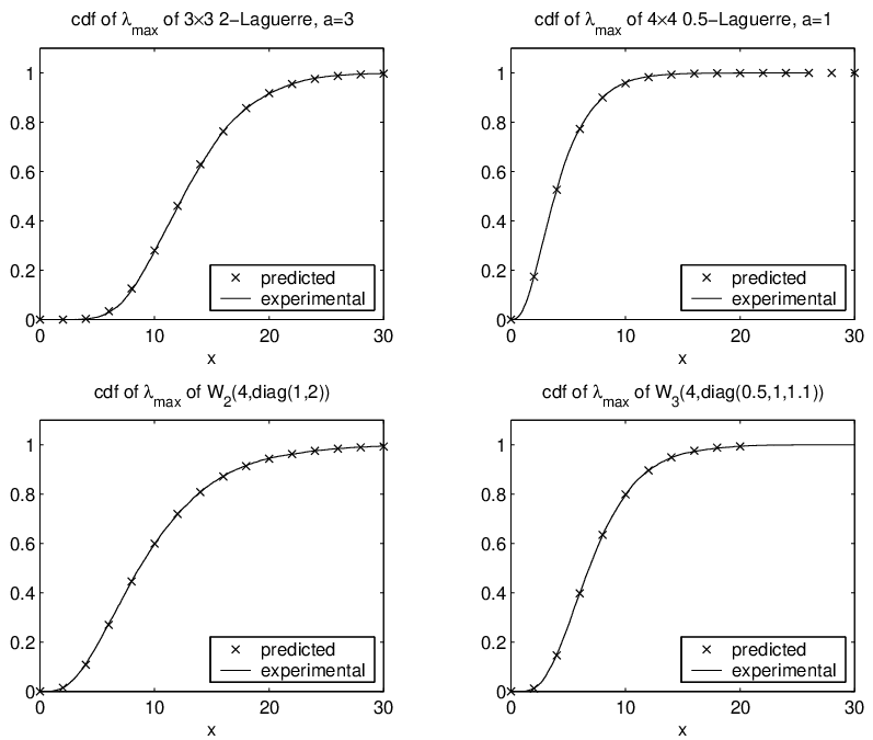
We performed extensive numerical tests to verify the correctness and complexity of our Algorithms 4.1 and 4.2. We compared the output of our algorithms for F0(α)0{}_{0}F^{{\mbox{\tiny$(\alpha)$}}}_{0} and F1(α)1{}_{1}F^{{\mbox{\tiny$(\alpha)$}}}_{1} with explicit expressions (subsection 6.1). We also compared the probability distributions of the eigenvalues of certain random matrices (which are expressed as hypergeometric functions) against the results of Monte–Carlo experiments (subsection 6.2). Finally, we present performance results in subsection 6.3.

6.1. Explicit Expressions

We compared the output of Algorithms 4.1 and 4.2 against the expressions [17, p. 262]:

F(α)00​(X)\phantom{{}^{(}}{}_{0}F_{0}^{{\mbox{\tiny$(\alpha)$}}}(X) =\displaystyle= etr​X;\displaystyle e^{{\rm tr}\,X}; (6.1)
F(α)01​(a,X)\phantom{{}^{(}}{}_{1}F_{0}^{{\mbox{\tiny$(\alpha)$}}}(a;X) =\displaystyle= det(I−X)−a,\displaystyle\det(I-X)^{-a}, (6.2)

for n=10n=10 and random uniformly distributed values xi∈[0,12]x_{i}\in[0,\frac{1}{2}], i=1,2,…,ni=1,2,\ldots,n. For m=30m=30 it took less than one second per test. The results agreed to at least 1212 decimal digits with (6.1), and at least 88 decimal digits with (6.2), reflecting the slower convergence of (6.2).

6.2. Eigenvalue Statistics

We tested Algorithms 4.1 and 4.2 against the eigenvalue statistics of the β\beta-Laguerre and Wishart matrices.

The n×nn\times n β\beta-Laguerre matrix of parameter aa is defined as L=B​BTL=BB^{T}, where

B=[χ2​aχβ⁡(n−1)χ2​a−β⋱⋱χβχ2​a−β⁡(n−1)],a>β2​(n−1).B=\left[\begin{array}[]{cccc}\chi_{2a}\\ \chi_{\beta(n-1)}&\chi_{2a-\beta}\\ &\ddots&\ddots\\ &&\chi_{\beta}&\chi_{2a-\beta(n-1)}\end{array}\right],\;\;\;a>\frac{\beta}{2}(n-1).

The n×nn\times n Wishart matrix with ll degrees of freedom (l>nl>n) and covariance matrix Σ\Sigma, A=Wn​(l,Σ)A=W_{n}(l,\Sigma), is defined as A=Σ1/2⋅ZT⋅Z⋅Σ1/2A=\Sigma^{1/2}\cdot Z^{T}\cdot Z\cdot\Sigma^{1/2}, where Zi​j=N⁡(0,1)Z_{ij}=N(0,1) for i=1,2,…,li=1,2,\ldots,l; j=1,2,…,nj=1,2,\ldots,n.

The eigenvalue distributions of AA and LL are the same when β=1\beta=1 or 22, a=l2a=\frac{l}{2}, and Σ=I\Sigma=I.

Refer to caption

Figure 1. The c.d.f. of λmax\lambda_{\max} of the β\beta-Laguerre matrix (top plots) and the Wishart matrix (bottom plots).

The cumulative distribution functions of the largest eigenvalues, λL\lambda_{L} and λA\lambda_{A}, of LL and AA, are

P⁡(λL<x)\displaystyle P(\lambda_{L}<x) =\displaystyle= Γn(α)​(n−1α+1)Γn(α)​(a+n−1α+1)​(x2)1a​n​F1(α)​(a,a+n−1α+1,−12​x​I),\displaystyle\frac{\Gamma_{n}^{{\mbox{\tiny$(\alpha)$}}}\big(\frac{n-1}{\alpha}+1\big)}{\Gamma_{n}^{{\mbox{\tiny$(\alpha)$}}}\big(a+\frac{n-1}{\alpha}+1\big)}\left(\frac{x}{2}\right)^{an}\!\!\phantom{{}^{2}}_{1}F_{1}^{{\mbox{\tiny$(\alpha)$}}}\big(a;a+{\textstyle\frac{n-1}{\alpha}+1;-\frac{1}{2}xI}\big),
P⁡(λA<x)\displaystyle P(\lambda_{A}<x) =\displaystyle= Γn(2)​(n+12)Γn(2)​(l+n+12)​det(12​x​Σ−1)1l/2​F1(2)​(l2,n+l+12,−12​x​Σ−1),\displaystyle\frac{\Gamma_{n}^{\mbox{\tiny$(2)$}}\big({\textstyle\frac{n+1}{2}}\big)}{\Gamma_{n}^{\mbox{\tiny$(2)$}}\big({\textstyle\frac{l+n+1}{2}}\big)}\det\big({\textstyle\frac{1}{2}}x\Sigma^{-1}\big)^{l/2}\!\!\phantom{{}^{2}}_{1}F_{1}^{\mbox{\tiny$(2)$}}\big({\textstyle\frac{l}{2}};{\textstyle\frac{n+l+1}{2}};-{\textstyle\frac{1}{2}}x\Sigma^{-1}\big),

respectively [4, Thm. 10.2.1, p. 147], [17, Thm. 9.7.1, p. 420], where α=2/β\alpha=2/\beta, and Γn(α)\Gamma_{n}^{{\mbox{\tiny$(\alpha)$}}} is the multivariate Gamma function of parameter α\alpha:

Γn(α)​(c)≡πn⁡(n−1)2​α​∏i=1nΓ⁡(c−i−1α)​ for ​ℜ⁡(c)>n−1α.\Gamma_{n}^{{\mbox{\tiny$(\alpha)$}}}(c)\equiv\pi^{\frac{n(n-1)}{2\alpha}}\prod_{i=1}^{n}\Gamma\left(c-\frac{i-1}{\alpha}\right)\mbox{~~~~for~~}\Re(c)>\frac{n-1}{\alpha}. (6.3)

We use the Kummer relation [17, Thm. 7.4.3, p. 265]

F(α)11​(a,c,X)=etr​X⋅1F1(α)​(c−a,c,−X)\phantom{{}^{\mbox{\tiny$(\alpha)$}}}{}_{1}F_{1}^{{\mbox{\tiny$(\alpha)$}}}(a;c;X)=e^{{\rm tr}\,X}\cdot\!\!\!\phantom{{}^{\mbox{\tiny$(\alpha)$}}}_{1}F_{1}^{{\mbox{\tiny$(\alpha)$}}}(c-a;c;-X)

to obtain the equivalent, but numerically more stable expressions

P⁡(λL<x)\displaystyle P(\lambda_{L}<x)\!\! =\displaystyle\!\!=\!\! Γn(α)​(n−1α+1)Γn(α)​(a+n−1α+1)​(x2)a​n​e1−n​x2​F1(α)​(n−1α+1,a+n−1α+1,12​x​I);\displaystyle\!\!\frac{\Gamma_{n}^{{\mbox{\tiny$(\alpha)$}}}\big(\frac{n-1}{\alpha}+1\big)}{\Gamma_{n}^{{\mbox{\tiny$(\alpha)$}}}\big(a+\frac{n-1}{\alpha}+1\big)}\left(\frac{x}{2}\right)^{an}e^{-\frac{nx}{2}}\!\!\phantom{{}^{2}}_{1}F_{1}^{{\mbox{\tiny$(\alpha)$}}}\big({\textstyle\frac{n-1}{\alpha}+1;a+\frac{n-1}{\alpha}+1;\frac{1}{2}xI}\big);
P⁡(λA<x)\displaystyle P(\lambda_{A}<x)\!\! =\displaystyle\!\!=\!\! Γn(2)​(n+12)Γn(2)​(l+n+12)​det(12​x​Σ−1)l/2​e1tr⁡(−x2​Σ−1)​F1(2)​(n+12,n+l+12,12​x​Σ−1),\displaystyle\!\!\frac{\Gamma_{n}^{\mbox{\tiny$(2)$}}\big({\textstyle\frac{n+1}{2}}\big)}{\Gamma_{n}^{\mbox{\tiny$(2)$}}\big({\textstyle\frac{l+n+1}{2}}\big)}\det\big({\textstyle\frac{1}{2}}x\Sigma^{-1}\big)^{l/2}e^{{\rm tr}(-\frac{x}{2}\Sigma^{-1})}\!\!\phantom{{}^{2}}_{1}F_{1}^{\mbox{\tiny$(2)$}}\big({\textstyle\frac{n+1}{2}};{\textstyle\frac{n+l+1}{2}};{\textstyle\frac{1}{2}}x\Sigma^{-1}\big),

which we plot on Figure 1 along with the Monte–Carlo results from a sample of 10000 random matrices.
Refer to caption

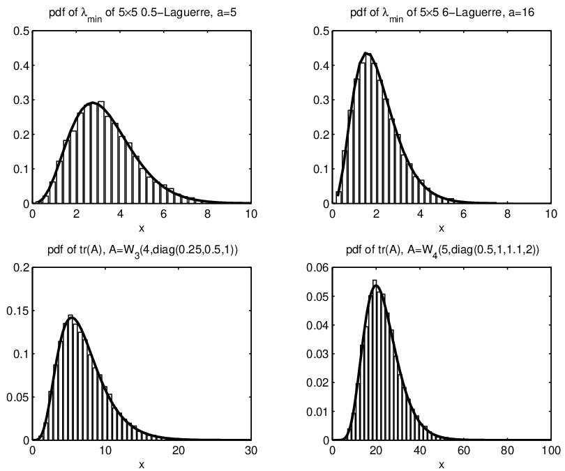
Figure 2. The p.d.f. of λmin\lambda_{\min} of the β\beta-Laguerre matrix (top plots) and the p.d.f. of the trace of the Wishart matrix (bottom plots).

Next we consider the distribution of the smallest eigenvalue of LL and that of tr​A{\rm tr}\,A.

If c=a−β2​(n−1)−1c=a-\frac{\beta}{2}(n-1)-1 is a nonnegative integer, then the probability density function of the smallest eigenvalue of LL is (see, e.g., [4, Thm. 10.1.1, p. 146]):

f(x)=xc​n⋅e−n​x2⋅2F0(2/β)(−c,βn2+1;−2xIn−1).f(x)=x^{cn}\cdot e^{-\frac{nx}{2}}\cdot\phantom{{}^{\beta}}_{2}F_{0}^{\mbox{\tiny$(2/\beta)$}}\big(-c,\beta\textstyle{\frac{n}{2}+1;-\frac{2}{x}I_{n-1}}\big). (6.4)

Since −c-c is a nonpositive integer, the series expansion of F(2/β)02\!\!\phantom{{}^{\mbox{\tiny$\beta$}}}{}_{2}F_{0}^{\mbox{\tiny$(2/\beta)$}} in (6.4) terminates, even though it diverges in general.

The probability density function of tr​A{\rm tr}\,A is

f⁡(u)\displaystyle f(u) =\displaystyle= det(λ−1Σ)−l/2∑k=0∞gl​n2+k,2​λ​(u)k!∑κ⊢k(l2)κ(2)⋅Cκ(2)(I−λΣ−1)\displaystyle\det(\lambda^{-1}\Sigma)^{-l/2}\sum_{k=0}^{\infty}\frac{g_{\frac{ln}{2}+k,2\lambda}(u)}{k!}\sum_{\kappa\vdash k}\big({\textstyle\frac{l}{2}}\big)_{\kappa}^{\mbox{\tiny$(2)$}}\cdot C_{\kappa}^{\mbox{\tiny$(2)$}}(I-\lambda\Sigma^{-1}) (6.5)
=\displaystyle= det(λ−1Σ)−l/2∑k=0∞gl​n2+k,2​λ(u)∑κ⊢k(l2)κ(2)2kjκ−1⋅Jκ(2)(I−λΣ−1),\displaystyle\det(\lambda^{-1}\Sigma)^{-l/2}\sum_{k=0}^{\infty}g_{\frac{ln}{2}+k,2\lambda}(u)\sum_{\kappa\vdash k}\big({\textstyle\frac{l}{2}}\big)_{\kappa}^{\mbox{\tiny$(2)$}}2^{k}j_{\kappa}^{-1}\cdot J_{\kappa}^{\mbox{\tiny$(2)$}}(I-\lambda\Sigma^{-1}),

where

gr,2​λ​(u)=e−u/2λur−1(2​λ)r​Γ​(r),(u>0),g_{r,2\lambda}(u)=\frac{e^{-u/2\lambda}u^{r-1}}{(2\lambda)^{r}\Gamma(r)},\;\;\;\;\;(u>0),

and λ\lambda is arbitrary [17, p. 341]. We follow the suggestion by Muirhead to use λ=2​λ1​λl/(λ1+λl)\lambda=2\lambda_{1}\lambda_{l}/(\lambda_{1}+\lambda_{l}), where λ1\lambda_{1} and λl\lambda_{l} are the largest and smallest eigenvalues of Σ\Sigma, respectively. Although the expression (6.5) is not a hypergeometric function of a matrix argument, its truncation for |κ|≤m|\kappa|\leq m has the form (1.6), and is computed analogously.

We plot (6.4) and (6.5) on Figure 2 and compare the theoretical predictions of these formulas with experimental data.

6.3. Performance Results

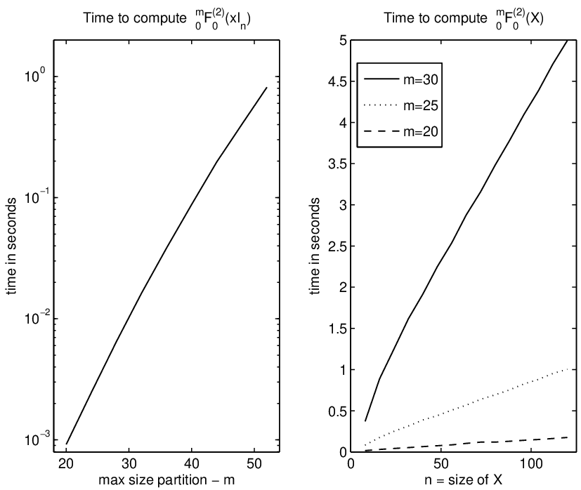
In Figure 3 we demonstrate the efficiency of Algorithms 4.1 and 4.2 on an 1.8GHz Intel Pentium 4 machine.

In the left plot we present the performance data for Algorithm 4.1 (whose complexity is independent of the size nn of the matrix X=x​IX=xI). Its efficiency is evident—we need to sum beyond partitions of size m=52m=52 before this algorithm takes a full second (for reference, the k!k! in the denominator of the κ\kappa-term in (1.1) then reaches up to 52!≈8⋅106752!\approx 8\cdot 10^{67}).

Algorithm 4.2 is also very efficient. The right plot of Figure 3 demonstrates clearly its linear complexity in nn. It also takes at most a few seconds on matrices of size n≤120n\leq 120 and partitions of size m≤30m\leq 30.

Refer to caption

Figure 3. The performance of Algorithms 4.1 (left) and 4.2 (right).

7. Conclusions and Open Problems

We have presented new algorithms for computing the truncation of the hypergeometric function of a matrix argument. They exploit the combinatorial properties of the Pochhammer symbol and the Jack function to achieve remarkable efficiency, and have lead to new results [1, 6].

Several problems remain open, among them automatic detection of convergence. The κ\kappa-term in (3.4) does approach zero as |κ|→∞|\kappa|\rightarrow\infty, but it need not monotonically decrease. Although we have

∏j=1κi−1(gj−α)​ejgj​(ej+α)⋅∏j=1i−1lj−fjlj+hj<1\prod_{j=1}^{\kappa_{i}-1}\frac{(g_{j}-\alpha)e_{j}}{g_{j}(e_{j}+\alpha)}\cdot\prod_{j=1}^{i-1}\frac{l_{j}-f_{j}}{l_{j}+h_{j}}<1

in (3.5), it is not always true that Qκ​Jκ(α)≤Qκ(i)​Jκ(i)(α)Q_{\kappa}J_{\kappa}^{{\mbox{\tiny$(\alpha)$}}}\leq Q_{\kappa_{(i)}}J_{\kappa_{(i)}}^{{\mbox{\tiny$(\alpha)$}}}, and it is unclear how to tell when convergence sets in.

Another open problem is to determine the best way to truncate the series (1.1). Our choice to truncate it for |κ|≤m|\kappa|\leq m seems to work well in practice, but one can imagine selecting a partition λ\lambda and truncating for κ≤λ\kappa\leq\lambda instead of, or in addition to |κ|≤m|\kappa|\leq m.

Acknowledgements

We thank Brian Sutton and Per-Olof Persson for several discussions that resulted in the simplification of the implementation of our algorithms, as well as the anonymous referee for the useful comments, which lead to improvements in the exposition.

References

  • [1] P.-A. Absil, A. Edelman, and P. Koev, On the largest principal angle between random subspaces, Submitted to Linear Algebra Appl., 2004.
  • [2] R. W. Butler and A. T. A. Wood, Laplace approximations for hypergeometric functions with matrix argument, Ann. Statist. 30 (2002), no. 4, 1155–1177.
  • [3] J. Demmel and P. Koev, Accurate and efficient evaluation of Schur and Jack functions, Math. Comp., to appear, 2005.
  • [4] I. Dumitriu, Eigenvalue statistics for the Beta-ensembles, Ph.D. thesis, Massachusetts Institute of Technology, 2003.
  • [5] I. Dumitriu and A. Edelman, Matrix models for beta ensembles, J. Math. Phys. 43 (2002), no. 11, 5830–5847.
  • [6] A. Edelman and B. Sutton, Tails of condition number distributions, SIAM J. Matrix Anal. Appl., accepted for publication, 2005.
  • [7] P. Forrester, Random matrix theory, 2001, preprint.
  • [8] H. Gao, P.J. Smith, and M.V. Clark, Theoretical reliability of MMSE linear diversity combining in Rayleigh-fading additive interference channels, IEEE Transactions on Communications 46 (1998), no. 5, 666–672.
  • [9] K. I. Gross and D. St. P. Richards, Total positivity, spherical series, and hypergeometric functions of matrix argument, J. Approx. Theory 59 (1989), no. 2, 224–246.
  • [10] R. Gutiérrez, J. Rodriguez, and A. J. Sáez, Approximation of hypergeometric functions with matricial argument through their development in series of zonal polynomials, Electron. Trans. Numer. Anal. 11 (2000), 121–130.
  • [11] G. H. Hardy, Ramanujan: Twelve lectures on subjects suggested by his life and work., AMS Chelsea, New York, 1999.
  • [12] M. Kang and M.-S. Alouini, Largest eigenvalue of complex Wishart matrices and performance analysis of MIMO MRC systems, IEEE Journal on Selected Areas in Communications 21 (2003), no. 3, 418–431.
  • [13] P. Koev, http://www-math.mit.edu/~plamen.
  • [14] I. G. Macdonald, Symmetric functions and Hall polynomials, Second ed., Oxford University Press, New York, 1995.
  • [15] The MathWorks, Inc., Natick, MA, MATLAB reference guide, 1992.
  • [16] R. J. Muirhead, Latent roots and matrix variates: a review of some asymptotic results, Ann. Statist. 6 (1978), no. 1, 5–33.
  • [17] by same author, Aspects of multivariate statistical theory, John Wiley & Sons Inc., New York, 1982.
  • [18] K. E. Muller, Computing the confluent hypergeometric function, M⁡(a,b,x)M(a,b,x), Numer. Math. 90 (2001), no. 1, 179–196.
  • [19] A. J. Sáez, Software for calculus of zonal polynomials,
    http://estio.ujaen.es/Profesores/ajsaez/software.html, 2004.
  • [20] R. Stanley, Some combinatorial properties of Jack symmetric functions, Adv. Math. 77 (1989), no. 1, 76–115.
  • [21] by same author, Enumerative combinatorics. Vol. 1, Cambridge Studies in Advanced Mathematics, vol. 49, Cambridge University Press, Cambridge, 1997.
  • [22] by same author, Enumerative combinatorics. Vol. 2, Cambridge Studies in Advanced Mathematics, vol. 62, Cambridge University Press, Cambridge, 1999.