T-homotopy and refinement of observation (II) : Adding new T-homotopy equivalences

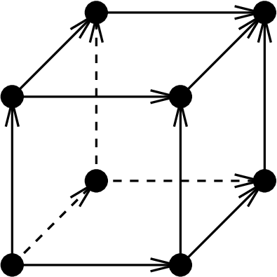
The first part [Gau05c] of this series was an expository paper about the geometric intuition underlying the notion of T-homotopy. The purpose of this second paper is to prove that the class of old T-homotopy equivalences introduced in [GG03] and in [Gau05a] is actually not big enough. Indeed, the only kind of old T-homotopy equivalence consists of the deformations which locally act like in Figure 1. So it becomes impossible with this old definition to identify the directed segment of Figure 1 with the full $3$-cube of Figure 2 by a zig-zag sequence of weak S-homotopy and of T-homotopy equivalences preserving the initial state and the final state of the $3$-cube since every point of the $3$-cube is related to three distinct edges. This contradicts the fact that concurrent execution paths cannot be distinguished by observation. The end of the paper proposes a new definition of T-homotopy equivalence following the paradigm of invariance by refinement of observation. It will be checked that the preceding drawback is then overcome.

This second part gives only a motivation for the new definition of T-homotopy. Further developments and applications are given in [Gau06b], [Gau06c] and [Gau06a]. The left-properness of the model category structure of [Gau03] is also established in this paper. The latter result is used several times in the next papers of this series (e.g., [Gau06b] Theorem 11.2, [Gau06c] Theorem 9.2).

Section 4 collects some facts about globular complexes and their relationship with the category of flows. Indeed, it is not known how to establish the limitations of the old form of T-homotopy equivalence without using globular complexes together with a compactness argument. Section 5 recalls the notion of old T-homotopy equivalence of flows which is a kind of morphism between flows coming from globular complexes (the class of flows ${\cell({\rm{\mathbf{Flow}}})}$). Section 6 presents elementary facts about relative $I^{gl}_{+}$-cell complexes which will be used later in the paper. Section 7 proves that the model category of flows is left proper. This technical fact is used in the proof of the main theorem of the paper, and it was not established in [Gau03]. Section 8 proves the first main theorem of the paper:

Finally Section 9 proposes a new definition of T-homotopy equivalence and the second main theorem of the paper is proved:

The initial object (resp. the terminal object) of a category $\mathcal{C}$, if it exists, is denoted by $\varnothing$ (resp. $\mathbf{1}$).

Let $\mathcal{C}$ be a cocomplete category. If $K$ is a set of morphisms of $\mathcal{C}$, then the class of morphisms of $\mathcal{C}$ that satisfy the RLP (right lifting property) with respect to any morphism of $K$ is denoted by $\inj(K)$ and the class of morphisms of $\mathcal{C}$ that are transfinite compositions of pushouts of elements of $K$ is denoted by $\cell(K)$. Denote by $\cof(K)$ the class of morphisms of $\mathcal{C}$ that satisfy the LLP (left lifting property) with respect to the morphisms of $\inj(K)$. It is a purely categorical fact that $\cell(K)\subset\cof(K)$. Moreover, every morphism of $\cof(K)$ is a retract of a morphism of $\cell(K)$ as soon as the domains of $K$ are small relative to $\cell(K)$ ([Hov99] Corollary 2.1.15). An element of $\cell(K)$ is called a relative $K$-cell complex. If $X$ is an object of $\mathcal{C}$, and if the canonical morphism $\varnothing\longrightarrow X$ is a relative $K$-cell complex, then the object $X$ is called a $K$-cell complex.

Let $\mathcal{C}$ be a cocomplete category with a distinguished set of morphisms $I$. Then let $\cell(\mathcal{C},I)$ be the full subcategory of $\mathcal{C}$ consisting of the object $X$ of $\mathcal{C}$ such that the canonical morphism $\varnothing\longrightarrow X$ is an object of $\cell(I)$. In other terms, $\cell(\mathcal{C},I)=(\varnothing\!\downarrow\!\mathcal{C})\cap\cell(I)$.

It is obviously impossible to read this paper without a strong familiarity with model categories. Possible references for model categories are [Hov99], [Hir03] and [DS95]. The original reference is [Qui67] but Quillen’s axiomatization is not used in this paper. The axiomatization from Hovey’s book is preferred. If $\mathcal{M}$ is a cofibrantly generated model category with set of generating cofibrations $I$, let $\cell(\mathcal{M}):=\cell(\mathcal{M},I)$: this is the full subcategory of cell complexes of the model category $\mathcal{M}$. A cofibrantly generated model structure $\mathcal{M}$ comes with a cofibrant replacement functor $Q:\mathcal{M}\longrightarrow\cell(\mathcal{M})$. In all usual model categories which are cellular ([Hir03] Definition 12.1.1), all the cofibrations are monomorphisms. Then for every monomorphism $f$ of such a model category $\mathcal{M}$, the morphism $Q(f)$ is a cofibration, and even an inclusion of subcomplexes ([Hir03] Definition 10.6.7) because the cofibrant replacement functor $Q$ is obtained by the small object argument, starting from the identity of the initial object. This is still true in the model category of flows reminded in Section 3 since the class of cofibrations which are monomorphisms is closed under pushout and transfinite composition.

A partially ordered set $(P,\leqslant)$ (or poset) is a set equipped with a reflexive antisymmetric and transitive binary relation $\leqslant$. A poset is locally finite if for any $(x,y)\in P\times P$, the set $[x,y]=\{z\in P,x\leqslant z\leqslant y\}$ is finite. A poset $(P,\leqslant)$ is bounded if there exist $\widehat{0}\in P$ and $\widehat{1}\in P$ such that $P=[\widehat{0},\widehat{1}]$ and such that $\widehat{0}\neq\widehat{1}$. For a bounded poset $P$, let $\widehat{0}=\min P$ (the bottom element) and $\widehat{1}=\max P$ (the top element). In a poset $P$, the interval $]\alpha,-]$ (the sub-poset of elements of $P$ strictly bigger than $\alpha$) can also be denoted by $P_{>\alpha}$.

A poset $P$, and in particular an ordinal, can be viewed as a small category denoted in the same way: the objects are the elements of $P$ and there exists a morphism from $x$ to $y$ if and only if $x\leqslant y$. If $\lambda$ is an ordinal, a $\lambda$-sequence in a cocomplete category $\mathcal{C}$ is a colimit-preserving functor $X$ from $\lambda$ to $\mathcal{C}$. We denote by $X_{\lambda}$ the colimit $\varinjlim X$ and the morphism $X_{0}\longrightarrow X_{\lambda}$ is called the transfinite composition of the morphisms $X_{\mu}\longrightarrow X_{\mu+1}$.

A model category is left proper if the pushout of a weak equivalence along a cofibration is a weak equivalence. The model categories ${\rm{\mathbf{Top}}}$ and ${\rm{\mathbf{Flow}}}$ (see below) are both left proper (cf. Theorem 7.4 for ${\rm{\mathbf{Flow}}}$).

In this paper, the notation means cofibration, the notation means fibration, the notation $\simeq$ means weak equivalence, and the notation $\cong$ means isomorphism.

The category ${\rm{\mathbf{Top}}}$ of compactly generated topological spaces (i.e. of weak Hausdorff $k$-spaces) is complete, cocomplete and cartesian closed (more details for this kind of topological spaces in [Bro88, May99], the appendix of [Lew78] and also the preliminaries of [Gau03]). For the sequel, any topological space will be supposed to be compactly generated. A compact space is always Hausdorff.

The category ${\rm{\mathbf{Top}}}$ is equipped with the unique model structure having the weak homotopy equivalences as weak equivalences and having the Serre fibrations ²² 2 that is a continuous map having the RLP with respect to the inclusion $\mathbf{D}^{n}\times 0\subset\mathbf{D}^{n}\times[0,1]$ for any $n\geqslant 0$ where $\mathbf{D}^{n}$ is the $n$-dimensional disk. as fibrations.

The time flow of a higher dimensional automaton is encoded in an object called a flow [Gau03]. A flow $X$ contains a set $X^{0}$ called the $0$-skeleton whose elements correspond to the states (or constant execution paths) of the higher dimensional automaton. For each pair of states $(\alpha,\beta)\in X^{0}\times X^{0}$, there is a topological space $\mathbb{P}_{\alpha,\beta}X$ whose elements correspond to the (non-constant) execution paths of the higher dimensional automaton beginning at $\alpha$ and ending at $\beta$. For $x\in\mathbb{P}_{\alpha,\beta}X$, let $\alpha=s(x)$ and $\beta=t(x)$. For each triple $(\alpha,\beta,\gamma)\in X^{0}\times X^{0}\times X^{0}$, there exists a continuous map $*:\mathbb{P}_{\alpha,\beta}X\times\mathbb{P}_{\beta,\gamma}X\longrightarrow\mathbb{P}_{\alpha,\gamma}X$ called the composition law which is supposed to be associative in an obvious sense. The topological space $\mathbb{P}X=\bigsqcup_{(\alpha,\beta)\in X^{0}\times X^{0}}\mathbb{P}_{\alpha,\beta}X$ is called the path space of $X$. The category of flows is denoted by ${\rm{\mathbf{Flow}}}$. A point $\alpha$ of $X^{0}$ such that there are no non-constant execution paths ending at $\alpha$ (resp. starting from $\alpha$) is called an initial state (resp. a final state). A morphism of flows $f$ from $X$ to $Y$ consists of a set map $f^{0}:X^{0}\longrightarrow Y^{0}$ and a continuous map $\mathbb{P}f:\mathbb{P}X\longrightarrow\mathbb{P}Y$ preserving the structure. A flow is therefore “almost” a small category enriched in ${\rm{\mathbf{Top}}}$. A flow $X$ is loopless if for every $\alpha\in X^{0}$, the space $\mathbb{P}_{\alpha,\alpha}X$ is empty.

Here are four fundamental examples of flows:

1. (1)

   Let $S$ be a set. The flow associated with $S$, still denoted by $S$, has $S$ as set of states and the empty space as path space. This construction induces a functor ${\rm{\mathbf{Set}}}\rightarrow{\rm{\mathbf{Flow}}}$ from the category of sets to that of flows. The flow associated with a set is loopless.

2. (2)

   Let $(P,\leqslant)$ be a poset. The flow associated with $(P,\leqslant)$, and still denoted by $P$ is defined as follows: the set of states of $P$ is the underlying set of $P$; the space of morphisms from $\alpha$ to $\beta$ is empty if $\alpha\geqslant\beta$ and equals to $\{(\alpha,\beta)\}$ if $\alpha<\beta$ and the composition law is defined by $(\alpha,\beta)*(\beta,\gamma)=(\alpha,\gamma)$. This construction induces a functor ${\rm{\mathbf{PoSet}}}\rightarrow{\rm{\mathbf{Flow}}}$ from the category of posets together with the strictly increasing maps to the category of flows. The flow associated with a poset is loopless.

3. (3)

   The flow ${\rm{Glob}}(Z)$ defined by

   	$\displaystyle{\rm{Glob}}(Z)^{0}=\{\widehat{0},\widehat{1}\}$
   	$\displaystyle\mathbb{P}{\rm{Glob}}(Z)=Z\hbox{ with }s(z)=\widehat{0}\hbox{ and }t(z)=\widehat{1}\hbox{ for all }z\in Z$

   and a trivial composition law (cf. Figure 3). It is called the globe of $Z$.

4. (4)

   The directed segment $\overrightarrow{I}$ is by definition ${\rm{Glob}}(\{0\})\cong\{\widehat{0}<\widehat{1}\}$.

The category ${\rm{\mathbf{Flow}}}$ is equipped with the unique model structure such that [Gau03]:

• •

  The weak equivalences are the weak S-homotopy equivalences, i.e. the morphisms of flows $f:X\longrightarrow Y$ such that $f^{0}:X^{0}\longrightarrow Y^{0}$ is a bijection and such that $\mathbb{P}f:\mathbb{P}X\longrightarrow\mathbb{P}Y$ is a weak homotopy equivalence.

• •

  The fibrations are the morphisms of flows $f:X\longrightarrow Y$ such that $\mathbb{P}f:\mathbb{P}X\longrightarrow\mathbb{P}Y$ is a Serre fibration.

This model structure is cofibrantly generated. The set of generating cofibrations is the set $I^{gl}_{+}=I^{gl}\cup\{R:\{0,1\}\longrightarrow\{0\},C:\varnothing\longrightarrow\{0\}\}$ with

where $\mathbf{D}^{n}$ is the $n$-dimensional disk and $\mathbf{S}^{n-1}$ the $(n-1)$-dimensional sphere. The set of generating trivial cofibrations is

If $X$ is an object of $\cell({\rm{\mathbf{Flow}}})$, then a presentation of the morphism $\varnothing\longrightarrow X$ as a transfinite composition of pushouts of morphisms of $I^{gl}_{+}$ is called a globular decomposition of $X$.

The reference is [Gau05a]. A globular complex is a topological space together with a structure describing the sequential process of attaching globular cells. A general globular complex may require an arbitrary long transfinite construction. We restrict our attention in this paper to globular complexes whose globular cells are morphisms of the form ${\rm{Glob}}^{top}(\mathbf{S}^{n-1})\longrightarrow{\rm{Glob}}^{top}(\mathbf{D}^{n})$ (cf. Definition 4.2).

The category of multipointed spaces is cocomplete.

Let $X$ be a globular precomplex. The $0$-skeleton of $\varinjlim X$ is equal to $X^{0}$.

The following theorem is important for the sequel:

The old notion of T-homotopy equivalence for globular complexes was given in [GG03]. A notion of T-homotopy equivalence of flows was given in [Gau05a] and it was proved in the same paper that these two notions are equivalent.

We first recall the definition of the branching and merging space functors, and then the definition of a T-homotopy equivalence of flows, exactly as given in [Gau05a] (Definition 5.7 below), and finally a characterization of T-homotopy of flows using globular complexes (Theorem 5.8 below).

Roughly speaking, the branching space of a flow is the space of germs of non-constant execution paths beginning in the same way.

Roughly speaking, the merging space of a flow is the space of germs of non-constant execution paths ending in the same way.

We recall the following important theorem for the sequel:

This characterization was actually the first definition of a T-homotopy equivalence proposed in [GG03] (see Definition 4.10 p66).

Recall that $I^{gl}_{+}=I^{gl}\cup\{R:\{0,1\}\longrightarrow\{0\},C:\varnothing\longrightarrow\{0\}\}$ with

Let $I_{g}=I^{gl}\cup\{C\}$. Since for any $n\geqslant 0$, the inclusion $\mathbf{S}^{n-1}\subset\mathbf{D}^{n}$ is a closed inclusion of topological spaces, so an effective monomorphism of the category ${\rm{\mathbf{Top}}}$ of compactly generated topological spaces, every morphism of $I_{g}$, and therefore every morphism of $\cell(I_{g})$, is an effective monomorphism of flows as well (cf. also [Gau03] Theorem 10.6).

If the topological spaces $X_{i}$ for $1\leqslant i\leqslant p$ are cofibrant, then the continuous map $\id_{X_{1}}\times\dots\times f\times\dots\times\dots\times\id_{X_{p}}$ is a cofibration since the model category of compactly generated topological spaces is monoidal with the categorical product as monoidal structure. So in this case, the result follows from the left properness of this model category ([Hir03] Theorem 13.1.10). In the general case, $\id_{X_{1}}\times\dots\times f\times\dots\times\dots\times\id_{X_{p}}$ is not a cofibration anymore. But any cofibration $f$ for the Quillen model structure of ${\rm{\mathbf{Top}}}$ is a cofibration for the Strøm model structure of ${\rm{\mathbf{Top}}}$ [Str66] [Str68] [Str72] [Col06]. In the latter model structure, any space is cofibrant. Therefore the continuous map $\id_{X_{1}}\times\dots\times f\times\dots\times\dots\times\id_{X_{p}}$ is a cofibration of the Strøm model structure of ${\rm{\mathbf{Top}}}$, that is a NDR pair. So the continuous map $\id_{X_{1}}\times\dots\times f\times\dots\times\dots\times\id_{X_{p}}$ is a closed $T_{1}$-inclusion anyway. This fact will be used below.

If for all $\mu<\lambda$, the continuous maps $M_{\mu}\longrightarrow M_{\mu+1}$ and $N_{\mu}\longrightarrow N_{\mu+1}$ are cofibrations, then Proposition 7.3 above is a consequence of [Hir03] Proposition 17.9.3 and of the fact that the model category ${\rm{\mathbf{Top}}}$ is left proper. With the same additional hypotheses, Proposition 7.3 above is also a consequence of [DI04] Theorem A.7. Indeed, the latter states that an homotopy colimit can be calculated either in the usual Quillen model structure of ${\rm{\mathbf{Top}}}$, or in the Strøm model structure of ${\rm{\mathbf{Top}}}$ [Str72] [Col06].

References

• [Bro88] R. Brown. Topology. Ellis Horwood Ltd., Chichester, second edition, 1988. A geometric account of general topology, homotopy types and the fundamental groupoid.
• [Col06] M. Cole. Many homotopy categories are homotopy categories. Topology Appl., 153(7):1084–1099, 2006.
• [DI04] D. Dugger and D. C. Isaksen. Topological hypercovers and 𝔸1\mathbb{A}^{1}-realizations. Math. Z., 246(4):667–689, 2004.
• [DS95] W. G. Dwyer and J. Spaliński. Homotopy theories and model categories. In Handbook of algebraic topology, pages 73–126. North-Holland, Amsterdam, 1995.
• [Gau03] P. Gaucher. A model category for the homotopy theory of concurrency. Homology, Homotopy and Applications, 5(1):p.549–599, 2003.
• [Gau05a] P. Gaucher. Comparing globular complex and flow. New York Journal of Mathematics, 11:p.97–150, 2005.
• [Gau05b] P. Gaucher. Homological properties of non-deterministic branchings and mergings in higher dimensional automata. Homology, Homotopy and Applications, 7(1):p.51–76, 2005.
• [Gau05c] P. Gaucher. T-homotopy and refinement of observation (I) : Introduction. ArXiv​:math.AT/0505152, to appear in ENTCS, 2005.
• [Gau06a] P. Gaucher. Inverting weak dihomotopy equivalence using homotopy continuous flow. Theory Appl. Categ., 16:No. 3, 59–83 (electronic), 2006.
• [Gau06b] P. Gaucher. T-homotopy and refinement of observation (III) : Invariance of the branching and merging homologies. New York J. Math., 12:319–348 (electronic), 2006.
• [Gau06c] P. Gaucher. T-homotopy and refinement of observation (IV) : Invariance of the underlying homotopy type. New York J. Math., 12:63–95 (electronic), 2006.
• [GG03] P. Gaucher and E. Goubault. Topological deformation of higher dimensional automata. Homology, Homotopy and Applications, 5(2):p.39–82, 2003.
• [Hig71] P. J. Higgins. Notes on categories and groupoids. Van Nostrand Reinhold Co., London, 1971. Van Nostrand Rienhold Mathematical Studies, No. 32.
• [Hir03] P. S. Hirschhorn. Model categories and their localizations, volume 99 of Mathematical Surveys and Monographs. American Mathematical Society, Providence, RI, 2003.
• [Hov99] M. Hovey. Model categories. American Mathematical Society, Providence, RI, 1999.
• [Lew78] L. G. Lewis. The stable category and generalized Thom spectra. PhD thesis, University of Chicago, 1978.
• [May99] J. P. May. A concise course in algebraic topology. University of Chicago Press, Chicago, IL, 1999.
• [Qui67] D. G. Quillen. Homotopical algebra. Springer-Verlag, Berlin, 1967.
• [Str66] A. Strøm. Note on cofibrations. Math. Scand., 19:11–14, 1966.
• [Str68] A. Strøm. Note on cofibrations. II. Math. Scand., 22:130–142 (1969), 1968.
• [Str72] A. Strøm. The homotopy category is a homotopy category. Arch. Math. (Basel), 23:435–441, 1972.