New topologically slice knots
Abstract
In the early 1980’s Mike Freedman showed that all knots with trivial Alexander polynomial are topologically slice (with fundamental group ). This paper contains the first new examples of topologically slice knots. In fact, we give a sufficient homological condition under which a knot is slice with fundamental group . These two fundamental groups are known to be the only solvable ribbon groups. Our homological condition implies that the Alexander polynomial equals but also contains information about the metabelian cover of the knot complement (since there are many non-slice knots with this Alexander polynomial).
keywords
Slice knots, surgery, Blanchfield pairingDepartment of Mathematics, University of California
Berkeley, CA 94720, USA \gtemail\mailtofriedl@rice.edu\quaand\qua\mailtoteichner@math.berkeley.edu
57M25 \secondaryclass57M27, 57N70
eometry & opology Volume 9 (2005) 2129–2158\nlPublished: 4 November 2005
Email:\stdspace\theemail
URL:\stdspace\theurl
Abstract
AMS Classification numbers Primary: \theprimaryclass
Secondary: \thesecondaryclass
Keywords: \thekeywords
Proposed: Robion Kirby Received: 12 May 2005\nlSeconded: Cameron Gordon, Wolfgang Lueck Accepted: 10 October 2005
1 Introduction
A knot is an embedding . We work in the topological category and assume that every embedding is locally flat. Note that a smooth embedding is locally flat and that we prefer to add the adjective “smooth” to emphasize this stronger condition on the embedding, except in our title. Two knots are called concordant if there exists an embedding which restricts to the given knots at both ends. The concordance classes form an abelian group under connected sum, the knot concordance group . A knot is called slice if it is concordant to the unknot or, equivalently, if it bounds an embedding of disks . Predating the 4–dimensional revolution in the early 80’s, Casson and Gordon showed that the epimorphism from onto its high dimension analogue has a nontrivial kernel [2]. There has been much recent progress in understanding how complicated really is. In [5], [6] an infinite sequence of new invariants was found using non-commutative Blanchfield forms and their von Neumann signatures. On the other hand, many knots are known to be slice, for example the knots in Figure 1.1, where the band can be tied into an arbitrary knot .

In fact, there is a large class of slice knots given as the boundary of ribbons in . These knots are called ribbon knots, where a ribbon is a smooth immersion such that all singularities are of the type as in Figure 1.2: They consist of arcs of self–intersection that lie completely in the interior of one of the two sheets involved. Such singularities can be resolved in by pushing an open disk around each singular arc slightly away from . Thus a ribbon leads to a smooth slice disk in , the so called ribbon disk. It is a fascinating open problem whether every smoothly slice knot is ribbon. One distinctive feature of a ribbon knot is that the inclusion map induces an epimorphism of the knot group onto the ribbon group, the fundamental group of the complement in of the ribbon disk. There is a simple criterion for a given group to be ribbon in terms of certain presentations, see Theorem 2.1. For general slice complements the inclusion map does not induce an epimorphism, and slice disks with the ontoness property are called homotopically ribbon, or h–ribbon for short.

In the topological category, Freedman proved that any knot with trivial Alexander polynomial is slice [10], see also [13] for a more direct construction. Using gauge theory, Gompf showed that some of these knots are not smoothly slice [14]. The easiest such knot is probably the Whitehead double of the trefoil knot, already exhibiting the subtle difference between smooth and topological 4–manifolds. In an amazing turn of events, Rasmussen very recently gave the first purely combinatorial proof for the fact that this knot is not smoothly slice. He constructed a concordance invariant from Khovanov homology [28] with beautiful properties. In particular, the arguments of [22] for showing that (iterated) Whitehead doubles of the trefoil are not smoothly slice can be adapted to this setting from the concordance invariant of Ozsváth and Szabó [23]. Livingston uses the following argument, going back to at least Rudolph: One can exhibit some Whitehead doubles as separating curves on minimal Seifert surfaces of certain torus knots. Since the Rasmussen and Ozsváth–Szabó invariants detect the minimal genus of torus knots, it follows that such separating curves cannot be smoothly slice.
In this note we provide the first new class of slice knots since Freedman’s construction, using his theorem [9] that solvable groups are good (for topological surgery). Our main result is the following theorem. Let
Here the generator of acts on the normal subgroup via multiplication by . It is known, cf Lemma 2.2, that and are the only solvable ribbon groups, hence the name. In geometric group theory, this group is also known as the Baumslag–Solitar group .
Theorem 1.3.
Let be a knot and denote by the –surgery on . If there is an epimorphism , or , such that
| (Ext) |
then is (topologically) slice. In fact, is h–ribbon with group if and only if this Ext–condition holds for some epimorphism .
The case is actually just a reformulation of Freedman’s theorem because the condition (Ext) is then equivalent to . For , we shall show in Corollary 3.4 that this condition implies
There are well known knots with this Alexander polynomial that are not slice (cf Section 7) so the h–ribbon question with group is more subtle than for . Our result complements work of Tim Cochran and Taehee Kim [7]. They show that if the degree of the Alexander polynomial is greater than two, than the homology of solvable covers can not determine whether a given knot is slice or not.
Remark.
We will show in Lemma 5.1 that the somewhat awkward (Ext) condition can be replaced by the condition that a non-commutative Blanchfield pairing
vanishes, where denotes the Ore localization of .
It is surprisingly easy to construct many knots that satisfy all conditions of our Theorem 1.3. For example, all knots in Figure 1.1 do. The easiest one is the knot , which is isotopic to the case where the band is the unknot. However, all knots in Figure 1.1 are obviously ribbon and hence we need to work harder to get new h–ribbon knots. One trick is the following satellite construction that can be considered as an analogue of Whitehead doubling (a nice way to obtain knots with trivial Alexander polynomial). We give a much more general result in Section 6.
Theorem 1.4.
Start with the knot , drawn in a solid torus as on the right hand side of Figure 1.5. Tie an arbitrary knot into that solid torus to obtain a satellite of . Then satisfies the assumptions of Theorem 1.3 and is therefore h–ribbon.
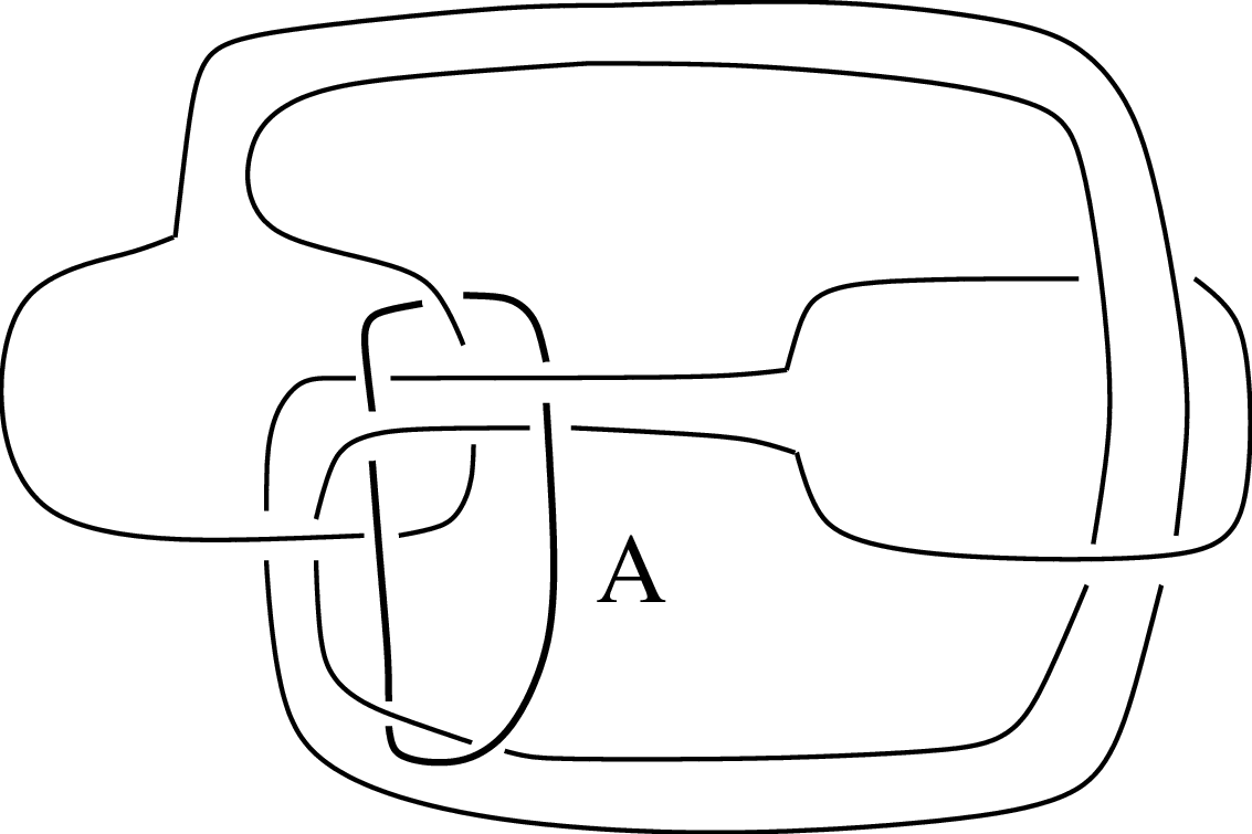

On the left hand side of Figure 1.5 we picked an axis which is unknotted in (so that the complement of will be a solid torus) and which punctures all ribbon disks that we could see. Then we redrew the picture in a way that becomes the meridian to the visible solid torus. We conjecture that Theorem 1.4 gives new examples of knots which are h–ribbon but not smoothly slice. The simplest candidate is the satellite knot of the trefoil knot. It has a knot diagram with 93 crossings and we are unable to compute Rasmussen’s invariant [28], the complexity of which is exponential in the number of crossings. For the general ribbon case we propose the following generalization of Theorem 1.3.
Conjecture 1.6.
Let be a ribbon group for which topological surgery works. A knot is h–ribbon with group if and only if there exists an epimorphism such that the condition (Ext) from Theorem 1.3 holds.
Note that the converse of this conjecture is not completely straight forward either. We use a Blanchfield form to prove the converse for the groups and .
Question 1.7.
Are the fundamental groups of complements of h–ribbons ribbon groups?
The phrase “surgery works for ” means here that the (reduced) surgery sequence
| () |
is exact for all Poincaré pairs with , see [10, chapter 11.3] for more information. If or then this sequence is exact by Freedman’s disk embedding theorem (cf [9] and [11]) for solvable groups. The general case is still open and since most other ribbon groups contain free groups we need a very strong form of this result. It is logically possible that topological surgery works for a given fundamental group but the disk embedding theorem (and hence the s–cobordism theorem) fail for this group.
The “if”–direction of Conjecture 1.6 would follow from the following purely homological conjecture. We say that satisfies the Poincaré duality condition if the induced inclusion is a finite 4–dimensional Poincaré pair.
Conjecture 1.8.
Let be a knot with an epimorphism onto a ribbon group such that the condition (Ext) from Theorem 1.3 holds. Then satisfies the Poincaré duality condition. Moreover, .
We give supporting evidence for this algebraic conjecture at the end of Section 2. For it is true out of easy reasons and in Lemmas 3.3, 4.1 and Lemma 4.4 we prove that the conjecture is true for . The main reason why this works is the fact that the group ring is an Ore-domain and hence has an ordinary (skew) quotient field, see Section 4. We use various lemmas and ideas from [5]. The first statement of Theorem 1.3 is then a consequence of the following general result.
Theorem 1.9.
Theorem 1.9 comes from the fact that given a Poincaré pair, one can attempt to use classical surgery theory to find a –manifold of type . We show that in the situation above, this approach successfully produces a h–ribbon complement that is a .
The paper is organized as follows. In Section 2 we recall several known facts about ribbon groups. In Section 3 we explain how surgery can be used to find h–ribbons. We accumulate several restrictions on the group , and in Section 4 we show that the group satisfies all of them. In Section 5 we will show that for our groups the (Ext)–condition can be replaced by a vanishing condition on a non–commutative Blanchfield pairing. In Section 6 we recall the satellite construction which we use to give examples of topologically slice knots in Section 7.
Acknowledgments\quaWe thank Chuck Livingston and the referee for their valuable comments on the first version of this paper. We also wish to thank Jerry Levine and Andrew Ranicki for helpful discussions regarding certain technical aspects in this paper.
The first author was partially supported by RTN Network HPRN-CT-2002-00287: Algebraic K–Theory, Linear Algebraic Groups and Related Structures. The second author is partially supported by NSF Grant DMS-0453957.
2 Ribbon disk complements
Definition.
A group is called ribbon if there exists a ribbon disk , as explained in the introduction, with .
The deficiency of a presentation of a group is the number of generators minus the number of relations. The deficiency of a finitely presented group is the maximum of the deficiencies of all presentations. The following theorem is well-known and uses the fact that any ribbon in 3–space can be obtained as follows: Start with an –component unlink and add bands to produce a knot, where the bands can be arbitrarily twisted and linked. In particular, the bands may hit the disks bounding the unlink which introduces our ribbon singularities. This description actually gives an embedded disk with a Morse function which has minima and saddles when restricted to . This implies that the complement , an open tubular neighborhood of , has a handle decomposition with one –handle, 1–handles and 2–handles, giving the desired group presentation.
Theorem 2.1.
A group is ribbon if and only if and has a Wirtinger presentation of deficiency one, ie, has a presentation of the form
where for some and .
Using the above theorem and the Wirtinger presentation, one sees that knot groups are ribbon. As pointed out by John Stallings, a direct geometric way to see the corresponding ribbon disk is as follows. Represent the knot by an arc ending in a plane . A rotation by 180 degrees in , with fixed plane , sweeps out a disk in which has the same local minima and saddles as the original knotted arc (when projected orthogonally to the fixed plane) and there are no maxima. Applying this construction to a knot , one obtains a ribbon disk with fundamental group and boundary . We recover by this argument the reason why the mirror image is the inverse of in the concordance group.
Lemma 2.2.
The only solvable ribbon groups are and .
Proof.
Wilson [32] shows that every solvable group of deficiency one is isomorphic to for some . A direct computation shows that if and only if . These are exactly the two groups in the statement. Below we show that is indeed a ribbon group. ∎
We now show that does in fact appear as the fundamental group of a ribbon disk complement. Let be the ribbon disk given by Figure 1.1. The corresponding ribbon disk complement is given by the handle diagram of Figure 2.3, with two (dotted) 1–handles and one 2–handle. This is the case in the discussion above Theorem 2.1, see also [15, p. 213].

Note that with one gets
which is in fact independent of the knot that was tied into the band in Figure 1.1.
Remark.
Writing for the above ribbon knot, then is a satellite knot with companion and orbit . The knot is the knot of the standard knot table and we shall construct many more examples in this manner in Section 6.
Remark.
Since any ribbon group has a presentation of deficiency it is in particular an E–group (cf [30, p. 324]), hence is an E–group (cf [30, p. 302]). It follows from a result of Roushon [29, Corollary 4.6] in the case that that the derived series of never stabilizes, ie, for all (cf also [3]). This means that with few exceptions ribbon groups are neither solvable nor does their derived series stabilize.
The ribbon group conjecture
Alexander duality implies that ribbon groups satisfy and . We say that a group is aspherical if is a 2–complex. For a ribbon group this is the case if . It is conjectured that ribbon groups are aspherical. Note that this is in turn a special case of the Whitehead conjecture. This conjecture is known to be true for all knot groups since knot complements are aspherical by the sphere theorem. It is also known for all locally indicable ribbon groups (cf [16]), which in particular includes all ribbon groups with for some ordinal (cf also [30]). For some more examples cf [17]. In particular, we conjecture that a ribbon group has the property that
This conjecture clearly holds for aspherical ribbon groups. Furthermore we conjecture that for a ribbon group and an epimorphism , we always have
The relevance of these properties comes from Lemma 3.3 and Theorem 1.9. We will prove all these properties for in Lemma 4.1.
3 Proof of the Main Theorem 1.3
Let be a knot in and denote by the result of zero framed surgery along . The following is a well known slice criterion, see eg, [5]. For the “only if” direction one takes to be the complement in of a (thickened up) slice disk. For the “if” direction one uses Freedman’s solution of the topological Poincaré conjecture in dimension 4, in order to recognize as the –manifold union a 2–handle along a meridian for in .
Proposition 3.1.
A knot is slice if and only if bounds a –manifold with
- 1.
is normally generated by the image of a meridian for ,
- 2.
,
- 3.
,
Furthermore, is h–ribbon with group if and only if is replaced by
- (1-h)
is surjective.
Note that the first two conditions can always be satisfied, even with . However, to satisfy condition (3) as well, it is often necessary to make the fundamental group of more complicated. In fact, if (1)–(3) are satisfied for then has vanishing Alexander polynomial. Thus the main problem is to find a candidate for the fundamental group of .
3.1 Outline of the construction of W
To prove Theorem 1.3, we take our candidate for the fundamental group to be or . By assumption we have given an epimorphism and we would like to find a –manifold with boundary such that the inclusion induces . Since any ribbon group satisfies and , such a manifold would fulfill the conditions (1-h), (2) and (3) above. This means that we are in a classical surgery situation and we can follow the steps taken by many before us. Below, the steps are labelled by the section numbers where they will be worked out.
- (3.2)
First we seek conditions such that is a Poincaré pair. It turns out that exactly condition (Ext) from Theorem 1.3 arises.
- (3.3)
Secondly, we check that the Spivak normal bundle of this Poincaré pair has a linear reduction, ie, that there is a degree 1 normal map from a (smooth) manifold pair . In fact, we shall see that there is a unique normal cobordism class of such maps if we require, as we shall, that the signature of is zero.
- (3.4)
This normal map has surgery obstruction in the reduced L–group. Since this quadratic form is nothing but the intersection form on . We will verify in Lemma 4.4 that our L–group vanishes and hence the intersection form on is (stably) hyperbolic.
- (3.5)
Finally, since by assumption the surgery sequence for our fundamental groups is exact (in the topological category), one gets a topological manifold together with a homotopy equivalence . Hence we found our h–ribbon by Proposition 3.1.
In the following sections, we go through these steps one by one. We will not assume from the beginning that or but we shall add conditions on (and ) as we go, in turn proving Theorem 1.9. It will turn out that some of these conditions are known for all ribbon groups and some are conjectural. For the groups and we will prove all conditions in Section 4.
3.2 The Poincaré duality condition
We will use the following conventions. If is the universal cover then has a right –module structure. Given a left –module we can consider . Using the usual involution on group rings given by we can turn left –modules into right –modules. We define .
Definition.
[31]\quaLet be CW–complexes, write . Then is called a Poincaré pair of dimension if there exists , such that
are isomorphisms of –right modules. is called the fundamental homology class of .
Note that if is a Poincaré complex, then from the long exact homology and cohomology sequences it follows that
is an isomorphism as well. In our case, will be the 3–manifold so that the second condition on will be satisfied. Recall that we have an inclusion that induces an epimorphism of fundamental groups. For brevity we set
Recall that if is a finite 4–dimensional Poincaré pair, we say that satisfies the Poincaré duality condition.
Lemma 3.2.
Assume that satisfies and for . Then satisfies the Poincaré duality condition if and only if
is an isomorphism for .
Remark.
Proof.
We first show the “only if” direction. In that case . But for since this is the homology of the -cover of which is contractible since . The claim now follows from the long exact cohomology sequence with –coefficients. We now turn to the proof of the “if” direction. By the long exact homology sequence of , with –coefficients, and the vanishing of we can choose a class that maps to the fundamental class under the boundary map. Cap product with this class induces maps as in above and we need to check that they are isomorphisms. These maps are the left (or right) most vertical arrows in the commutative diagram of long exact sequences (with –coefficients understood):
Recall that for . Therefore, we need to show in particular that for . Note that
Since the maps are isomorphisms it suffices to show that for all the maps
are isomorphisms. For this is our assumption so it suffices to discuss the other cases. For both groups are zero since has infinite order. For again both groups are zero, for this is our assumption and for it follows from . Finally, we need to discuss the special case in the diagram above. Then
and by assumption for . It follows that the boundary map is an isomorphism and by commutativity of the diagram the last map in question
is also an isomorphism. ∎
Lemma 3.3.
Let satisfy and for . Furthermore, assume that for . Then satisfies the Poincaré duality condition if and only if the (Ext) condition from Theorem 1.3 holds: .
Proof.
Denote the universal cover of by . Write . Note that we have a chain isomorphism of right –module complexes given by
Therefore . We now apply the universal coefficient spectral sequence (UCSS). This has an –term
differentials of degree and converges to
cf [20, Theorem 2.7] for more details. We use that the edge homomorphism at of the spectral sequence is the map
By Lemma 3.2 we only need to verify that this is an isomorphism for if and only if condition (Ext) holds. For this follows immediately from our assumption . For we first observe that since there are no possible –differentials into the spot. Since , we get a short exact sequence
showing that the condition (Ext) holds if and only if is an isomorphism. ∎
Let be any group with . Then we define to be the order of the –module . Note that is well-defined up to multiplication by a unit in and up taking the natural involution . For example if , then .
Corollary 3.4.
Let and satisfy all the conditions from Lemma 3.3, including the (Ext) condition. Then
In particular .
Proof.
By Lemma 3.3 is a Poincaré pair. Since
for all it follows from a well-known argument that
for all . In particular is –torsion for all . The corollary now follows from the long exact sequence of with –coefficients, duality, and the fact that the alternating product of orders of a long exact sequence equals one (cf [19, Lemma 5, p. 76]). The Arf invariant of a knot has the well-known property that it equals zero if , and 1 otherwise. ∎
We shall now work through the remaining steps outlined in Section 3.1. We have a Poincaré pair where and . Clearly is normally generated by the image of a meridian for since is surjective and since any meridian normally generates . Furthermore and . It follows from the homology exact sequence of the pair , Poincaré duality, and the fact that is an isomorphism on that .
3.3 The degree 1 normal map
We show that the stable Spivak normal bundle of has a linear reduction. It seems well known to experts that this is always true in the oriented case in 4 dimensions but we could not find an explicit reference. So here is a rather ad hoc argument: Since is orientable, its tangent bundle is trivial and so is its stable normal bundle. We claim that the stable Spivak normal bundle of is also trivial: Let be the classifying space of such (oriented) bundles. Its homotopy groups are the (shifted) stable homotopy groups of spheres, starting with
It follows that for all we have which shows that the classifying map of the stable Spivak normal bundle is trivial. Finally, it is clear that, up to homotopy, this trivial map can be lifted (trivially) through the fibration , having the trivial map on the boundary . From the usual transversality theory we obtain a degree 1 normal map from a manifold pair
that is the identity on the boundary. Note that since the stable normal bundle of is trivial, so is that of . In particular, is spin. Another approach to finding is to prove that represents the zero element in the spin-bordism group . The fact that this element is zero comes from comparing with the Poincaré duality spin bordism group in which itself gives a zero bordism. Even though this is not really important for our main argument, we next show that is unique in a certain sense: In the spin case the normal cobordism group of degree 1 normal maps is isomorphic to
where the summand is the difference of ordinary signatures, . The first summand vanishes in our case and so does . By adding copies of Freedman’s –manifold to , we may assume that . This is just another way of saying that we work with the reduced normal cobordism group.
3.4 The surgery obstruction
There is a well defined surgery obstruction in which in our case is simply the intersection form on . The first step is ‘surgery below the middle dimension’ which makes 2–connected. The surgery obstruction then measures the kernel of in the middle dimension which in our case is in . To make this precise, recall the following definition from [31, p. 47].
Definition.
A quadratic form over is defined to be a triple with a free –module,
a non-singular hermitian form and
a quadratic refinement. Here a form is non-singular if the induced map is an isomorphism. A form isomorphic to a direct sum of the form , where and , is called a hyperbolic form.
It should be pointed out that in the oriented case, where the involution on is given by , the quadratic refinement is completely determined by the hermitian form . Its only role is to make sure that is even in the sense that for every there is an such that
| (even) |
The main examples of hermitian forms come from the intersection form of –manifolds, where and . If is represented by an immersed –sphere in , then one can look at the self-intersections that are related to the intersection of and a parallel push-off by the following formula:
Here denotes the normal Euler class of . Note that the coefficient of in can be changed arbitrarily by a (nonregular) homotopy, the so called cusp move. This also changes so as to make the above formula still hold (the left hand side only depends on the homotopy class of ). It follows that the intersection form on of a –manifold is even in the above sense if and only if is an even integer, ie, the second Stiefel–Whitney class vanishes. That is why we will completely ignore the quadratic refinement in the following, only making sure that our manifolds are spin. Note that for general spin –manifolds with fundamental group , the intersection form on is not a quadratic form in the above sense. The problems are that in general is not free and is not non-singular. However, given a –connected degree 1 map , one can restrict to the kernel of on . Then both of these conditions can be arranged after stabilizing by copies of , [31, p. 26]. Moreover, if vanishes on –spheres in this kernel then a quadratic refinement exists by the above considerations. If is a normal map (in addition to having degree 1) then this last condition is obvious. In our setting, so that we automatically work on the kernel of . Moreover, we saw that is spin so that the intersection form on is even and hence represents a unique quadratic form, up to the stabilization with hyperbolic forms. This motivates the following definition. Consider the semigroup of quadratic forms under direct sum. We say that forms are equivalent if there exist hyperbolic forms , such that and are isomorphic. The set of equivalence classes form a group (cf [27, p. 249]), denoted by . As discussed above, represents an element in this group.
Theorem 3.5.
The ordinary signature induces isomorphisms
- 1.
- 2.
for or .
The first statement is well-known, see for example [31, Theorem 13A.1]. The second statement is well-known in the case that (cf [26]). We prove the case in Section 4. In general if is a ribbon group, then is an isomorphism if the Whitehead conjecture and the Farrell–Jones conjecture hold. This has been shown in many interesting cases, cf [1] for the case of knot groups. By the computations in Section 3.3, the surgery obstruction actually only depends on the original data if we assume that , ie, that it lies in the reduced L–group
This element is hence an obstruction for finding a h–ribbon for with epimorphism . If the reduced L–group vanishes then, after further stabilization by , we may assume that has hyperbolic intersection form.
3.5 Constructing the h–ribbon disk
The assumptions of Theorem 1.9 say that the reduced L–group vanishes and that the topological surgery sequence is exact for our fundamental group. Therefore, one gets a topological manifold together with a homotopy equivalence . Hence we found our h–ribbon by Proposition 3.1 and we finished the proof of Theorem 1.9.
3.6 Proof of Theorem 1.3
To construct a ribbon disk we use Theorem 1.9 that we just finished proving. For , we will show all the required properties in Section 4. For they are easy to check, for example the conditions on follow from the fact that the Alexander module is a –torsion module. Moreover,
so that our (Ext) condition simply means that the Alexander module (or, equivalently, the Alexander polynomial) of is trivial. Conversely, assume that there exists a h–ribbon for with . Then it follows from arguments as in the proof of Theorem 4.4 in [5] that the Blanchfield form always vanishes on
In our case this group equals since . In the Section 5 we will recall this Blanchfield form and show in Lemma 5.1 that its vanishing is indeed equivalent to our (Ext) condition.
4 Properties of the solvable ribbon group
The purpose of this section is to prove that the assumptions of Lemma 3.3 are satisfied for the group :
Lemma 4.1.
The group satisfies and for . Furthermore, for any knot and any epimorphism one has
A group is called poly-torsion-free-abelian (PTFA) if there exists a filtration
such that is torsion free abelian. As we pointed out in Section 2 the only solvable ribbon groups are and and clearly both are PTFA. If is a PTFA group then the group ring satisfies the Ore condition and therefore has an Ore localization, cf [5, Proposition 2.5]
which is a skew field. Therefore, every –module is free and its rank is well-defined. As a localization, is flat as a right (and left) –module. Moreover, the –torsion part of a module is a submodule (unlike for general non-commutative rings). Let be a knot and be an epimorphism onto a PTFA group. From [5, Proposition 2.11] it follows that
ie, is –torsion. In particular, the required condition
in Lemma 4.1 follows. Furthermore,
and similarly since . The Euler characteristics of with and coefficients agree by the usual argument and hence
It follows that
Therefore and hence because is again –torsion. So another required condition in Lemma 4.1 follows:
The following result finishes up our task of showing has all the required properties.
Lemma 4.2.
The group is aspherical, in particular for and .
Proof.
Let be a ribbon disk with complement and fundamental group . Recall that by Alexander duality . We will show that is a . First note that is homotopy equivalent to a 2–complex . By the Hurewicz theorem it suffices to prove the vanishing of . Let be the Ore localization of . By the same arguments as above for , involving Euler characteristics, one shows that
Now consider the following commutative diagram
The second vertical map is injective since is a free –module, hence the first vertical map is injective as well, hence . ∎
Remark.
We could have used the well known fact that a one-relator group is aspherical if the relation is not a proper power (so in particular the group is torsion free). However, a similar argument as above will also be used in the proof of Lemma 4.3. Locally indicable ribbon groups are also known to be aspherical.
The following result is not needed in the rest of the paper but we include it for the interested reader. The nontriviality of the homology group in question made it clear that some more naive formulations of the Poincaré duality condition must fail. Recall from Section 2 that has the presentation
Lemma 4.3.
Let , then maps onto . More precisely, as a right –module, is the quotient of by the right ideal generated by
Dividing by the two-sided ideal generated by the same elements gives the ring .
Proof.
The proof of Lemma 4.1 shows that the 2–complex associated to the above presentation is a . Therefore, we can calculate from the short resolution
where the first map is given by the Fox derivatives and of the relation . A straightforward calculation using Fox derivatives ‘from the left’ gives
If we now decide to quotient by the two-sided ideal generated by the first relation, we find that the defining relation forces and hence we are left with , generated by . The second relation then introduces the relation into this commutative ring which gives the ring . ∎
Computation of
Lemma 4.4.
The inclusion map induces an isomorphism .
In order to prove this lemma, we need a theorem by Ranicki, which in turn needs the notion of –groups for any . We refer to [25] for the definition of these groups. We recall that the Whitehead group for a group is defined as (cf [27, p. 172] for a definition of ).
Theorem 4.5.
[24]\quaLet be a group with and let be an automorphism, then there exists a long exact sequence
where denotes the twisted Laurent ring, ie, for we have .
Remark.
Since , we don’t have to distinguish between and . We will therefore henceforth drop any decorations.
We’ll make use of the fact that is the direct limit of the direct system . We’ll therefore write . Denote the map by ; then .
Claim.
The determinant map is an isomorphism (cf [27, p. 172]). The functor commutes with direct limits and commutes with the determinant maps, hence is an isomorphism as well. It now follows immediately that .
By Theorem 4.5 there therefore exists an exact sequence
It is clear that the proposition follows once we prove the following claim.
Claim.
- 1.
is an isomorphism,
- 2.
is the identity map,
- 3.
We recall that (cf [31])
From Theorem 4.5 it follows that via the map induced by the inclusion . The inverse is given by tensoring with , considered as a –module via the map . In particular the map induces the identity on the group of the group ring, ie, on . From the fact that the –functor commutes with direct limits, we immediately get the first two statements. From [31, p. 181] we get the following commutative diagram
where denotes multiplication by two. In particular factors through . Hence is the zero map, taking direct limits we see that . This completes the proof of Lemma 4.4.
5 Non-commutative Blanchfield forms
Let be a PTFA–group and a homomorphism. Note that the involution on extends to an involution on and on . Let . Note that the map
is well–defined and induces an evaluation map
Now consider
ie, the composition of Poincaré duality, the inverse of the Bockstein homomorphism for the coefficient sequence and the above evaluation map.
Note that the second map is an isomorphism since the homology and hence the cohomology with coefficients vanishes. This map defines the hermitian Blanchfield pairing, cf [8, Theorem 5.1]
Lemma 5.1.
For or , the condition (Ext) from Theorem 1.3 is equivalent to the vanishing of the Blanchfield form .
The remark after Lemma 3.2 shows that the vanishing of the Blanchfield pairing is a weaker statement than the vanishing of the corresponding homology group . In particular, this shows that will in general be singular.
Proof of Lemma 5.1.
From the long exact –sequence corresponding to
it follows that
since for all (cf [5, Remark 2.8]). We are now done once we show that the homomorphism
| (5.2) |
in the definition of is surjective. As in the proof of Lemma 3.3 we have an isomorphism
Now applying the UCSS we see that the evaluation map (5.2) is surjective if . Let . By Lemma 4.2 we can assume that is a 2–complex. Then
Note that for , in particular it follows that
because is a 2–complex. ∎
Since is nonsingular for any knot , it vanishes if and only if the Alexander module itself vanishes. This in turn is equivalent to having trivial Alexander polynomial and to our condition (Ext) for .
6 The satellite construction
Let be knots. Let be a curve, unknotted in . Then is a solid torus. Let be a diffeomorphism which sends a meridian of to a longitude of , and a longitude of to a meridian of . The space
is a 3–sphere and the image of is denoted by . We say is the satellite knot with companion , orbit and axis . Note that we replaced a tubular neighborhood of by a knot in a solid torus, namely . Figure 6.1 shows that taking the Whitehead double of a knot is an example for the satellite construction.

It is easy to see that
Obstruction theory shows that the map can be extended to a map . Combining with the injection this defines a map . Let be a homomorphism onto a torsion-free group. Then we get an induced map .
Lemma 6.2.
If , then , otherwise
where is a module via .
Proof.
Consider the following commutative diagram of Meyer–Vietoris exact sequences (with –coefficients understood)
If , then the coefficient systems for and for are trivial, hence
This immediately implies that . If , then since is an element of infinite order since is torsion free. Furthermore is a free –module on the meridian of , which gets mapped to the longitude in which is zero in . From the above commutative diagram it now follows that
since . The lemma now follows from . ∎
7 Examples: Satellite knots of
In Figure 7.1 we see three projections of the knot , the first one having the minimal crossing number 6.

Indeed, the isotopy between and is shown in [2]. The isotopy between and follows from Figures 1.1 and 7.2, which shows that both knots are formed by band connected sum of two trivial knots along isotopic bands. Note that the two trivial circles in Figure 7.2 bound disjoint disks in .

Now consider the knot with the Seifert surface in Figure 7.3. With the given basis for we get
which then shows that .

Examples of h–ribbon knots
We first prove a general result. Let be a ribbon knot with ribbon disk , such that . Denote the induced map by . Let be any knot and the unknot in .
Proposition 7.4.
If then the satellite knot is h–ribbon.
Proof.
This result is similar to the well-known fact that the Whitehead double of any knot (which is the satellite of the unknot) is topologically slice. This is an immediate corollary from Freedman’s slicing theorem and Lemma 6.2.
Now turn back to the study of . From the discussion in Section 2 we know that has a ribbon disk such that . The group is generated by the meridians of . From Figure 2.3 it follows that the map
is given by the map indicated in Figure 7.5.

The image of the other meridians is determined by the image of the two given meridians.
As an example take , as in Figure 7.6 and the trefoil knot.
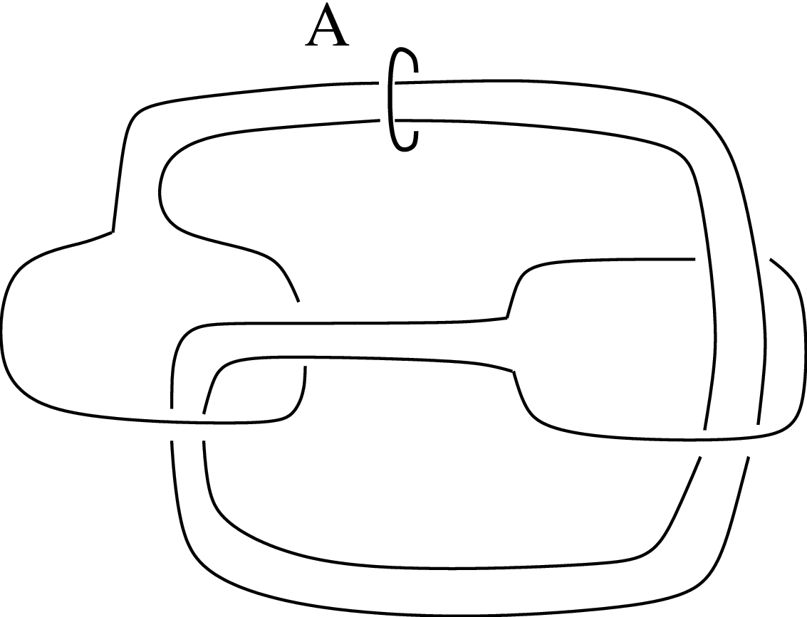

We have as one can easily verify. Therefore is h–ribbon by Proposition 7.4. But in fact is trivially ribbon already, since the ribbon disk of ‘survives’ the satellite construction. We therefore need a more subtle choice of . Now consider Figure 1.5. One can easily verify that . The knot as a knot in the torus is given in Figure 1.5 on the right. Wrapping this knot around say the trefoil gives a h–ribbon knot, which we conjecture not to be smoothly ribbon.
Remark.
It follows immediately from arguments as in Lemma 6.2 that
In particular and have the same abelian invariants. Livingston [21] showed that there exists a knot with
which is not topologically slice (cf also [18]). This shows that the vanishing of , which is a condition on the non-commutative homology of , can not be reduced to a condition on abelian invariants.
Non-existence of certain ribbon disks
Now consider the knot with the Seifert surface in Figure 7.3. For given knots consider , ie, the result of applying the satellite construction twice. This means that we tie knots and into the bands and .
Proposition 7.7.
If , then has no h–ribbon with fundamental group .
Proof.
Assume that has in fact a h–ribbon with fundamental group . Then is a metabolizer for (cf [12]). In the following we will write . Note that in Figure 7.3 lift to elements in , in fact
Furthermore the Blanchfield pairing is given by the matrix . It is easy to see that the submodule generated by respectively by are the only two metabolizers for . In particular the map is up to automorphism of either of the form
or it is of the same form with replaced by . We denote this homomorphism by . By Theorem 1.3 we get with –coefficients induced by or by . Now consider coefficients induced by . From Lemma 6.2 it follows that
We compute
Note that , in particular it is –torsion free. It follows from [20, Theorem 3.4] that , which is non-trivial since . The same calculation for then gives the contradiction. ∎
Non-uniqueness of ribbon groups
A ribbon knot can in general have ribbons with non-isomorphic groups. For example let be a non-trivial knot with , eg, the Whitehead double of a non-trivial knot. Let , then is in particular a ribbon group for the knot . On the other hand, still has trivial Alexander polynomial and so by Theorem 1.3 it follows that also has a h–ribbon with fundamental group . In fact, if is the Whitehead double of a ribbon knot then it is ribbon, not just h–ribbon, with fundamental group (and so is ).
References
- [1] C S Aravinda, F T Farrell, S K Roushon, Surgery groups of knot and link complements, Bull. London Math. Soc. 29 (1997) 400–406 \MR1446558
- [2] A J Casson, C M Gordon, Cobordism of classical knots, from: “À la recherche de la topologie perdue”, Progr. Math. 62, Birkhäuser Boston, Boston, MA (1986) 181–199 \MR900252
- [3] T D Cochran, Noncommutative knot theory, Algebr. Geom. Topol. 4 (2004) 347–398 \MR2077670
- [4] T D Cochran, K E Orr, P Teichner, Structure in the classical knot concordance group, Comment. Math. Helv. 79 (2004) 105–123 \MR2031301
- [5] T D Cochran, K E Orr, P Teichner, Knot concordance, Whitney towers and –signatures, Ann. of Math. (2) 157 (2003) 433–519 \MR1973052
- [6] T D Cochran, P Teichner, Knot concordance and von Neumann –invariants, preprint (2004)
- [7] T D Cochran, T Kim, Higher-order Alexander invariants and filtrations of the knot concordance group, preprint (2005)
- [8] J Duval, Forme de Blanchfield et cobordisme d’entrelacs bords, Comment. Math. Helv. 61 (1986) 617–635 \MR870709
- [9] M H Freedman, The topology of four-dimensional manifolds, J. Differential Geom. 17 (1982) 357–453 \MR679066
- [10] M H Freedman, F Quinn, Topology of –manifolds, Princeton Mathematical Series 39, Princeton University Press, Princeton, NJ (1990) \MR1201584
- [11] M H Freedman, P Teichner, –manifold topology. I. Subexponential groups, Invent. Math. 122 (1995) 509–529 \MR1359602
- [12] S Friedl, Eta invariants as sliceness obstructions and their relation to Casson–Gordon invariants, \agtref4200439893934 \MR2100685
- [13] S Garoufalidis, P Teichner, On knots with trivial Alexander polynomial, J. Differential Geom. 67 (2004) 167–193 \MR2153483
- [14] R E Gompf, Smooth concordance of topologically slice knots, Topology 25 (1986) 353–373 \MR842430
- [15] R E Gompf, A I Stipsicz, –manifolds and Kirby calculus, Graduate Studies in Mathematics 20, Amer. Math Soc. Providence, RI (1999) \MR1707327
- [16] J Howie, On locally indicable groups, Math. Z. 180 (1982) 445–461 \MR667000
- [17] J Howie, On the asphericity of ribbon disc complements, Trans. Amer. Math. Soc. 289 (1985) 281–302 \MR779064
- [18] T Kim, An infinite family of non-concordant knots having the same Seifert form, Comment. Math. Helv. 80 (2005) 147–155 \MR2130571
- [19] J Levine, A method for generating link polynomials, Amer. J. Math. 89 (1967) 69–84 \MR0224082
- [20] J Levine, Knot modules. I, Trans. Amer. Math. Soc. 229 (1977) 1–50 \MR0461518
- [21] C Livingston, Seifert forms and concordance, \gtref6200214403408 \MR1928840
- [22] C Livingston, Computations of the Ozsváth–Szabó knot concordance invariant, \gtref8200419735742 \MR2057779
- [23] P Ozsváth, Z Szabó, Knot Floer homology and the four-ball genus, \gtref7200317615639 \MR2026543
- [24] A A Ranicki, Algebraic –theory. III. Twisted Laurent extensions, from: “Algebraic K-theory, III”, SLN 343, Springer (1973) 412–463 \MR0414663
- [25] A A Ranicki, Algebraic –theory and topological manifolds, Cambridge Tracts in Mathematics 102, Cambridge University Press (1992) \MR1211640
- [26] A Ranicki, High-dimensional knot theory, Springer Monographs in Mathematics, Springer-Verlag, New York (1998) \MR1713074
- [27] A Ranicki, Algebraic and geometric surgery, Oxford Mathematical Monographs, Oxford University Press (2002) \MR2061749
- [28] J A Rasmussen, Khovanov homology and the slice genus, e-print (2004) \arxivmath.GT/0402131
- [29] S K Roushon, Topology of 3-manifolds and a class of groups II, preprint (2003)
- [30] R Strebel, Homological methods applied to the derived series of groups, Comment. Math. Helv. 49 (1974) 302–332 \MR0354896
- [31] C T C Wall, Surgery on compact manifolds, Mathematical Surveys and Monographs 69, Amer. Math. Soc. Providence, RI (1999) \MR1687388
- [32] J S Wilson, Soluble groups of deficiency , Bull. London Math. Soc. 28 (1996) 476–480 \MR1396147
Thiserratum was received and accepted on 6 September 2006 and published on 18 October 2006 as Geom. Topol. 10 (2006) 2501–2504.
\clCorrection to ‘New topologically slice knots’
Abstract\quaIn Figure 1.5 of [1] (above) we gave an incorrect example for Theorem 1.3. In this note we present a correct example.
We first recall the satellite construction for knots. Let be knots. Let be a curve, unknotted in . Then is a solid torus. Now let be a diffeomorphism which sends a meridian of to a longitude of , and a longitude of to a meridian of . The space
is a 3-sphere and the image of is denoted by . We say is the satellite knot with companion , orbit and axis . Note that by doing this construction we replaced a tubular neighborhood of by a knot in a solid torus, namely .
We now consider the knot in Figure 1.
at 56 68
\endlabellist
Note that is the knot . clearly bounds an immersed band; pushing this band into we can resolve the singularities to get a smooth slice disk for .
It follows from Proposition 7.4 that if is a curve such that represents an element in , then is topologically slice. We recall that is isomorphic to the semi–direct product
Here the generator of acts on the normal subgroup via multiplication by . In Figure 1.5 we proposed a curve and claimed that it represents the trivial element in . Unfortunately we miscalculated the image of in . In fact this represents a non–trivial element in . Hence the curve of Figure 1.5 does not give an example for Proposition 7.4. We now present a correct example.
Perhaps the first example of a pair which satisfies the above conditions which comes to mind is to take which form a slice link . But it is easy to see that the null–concordance from to a trivial link induces a concordance of to . But clearly is the trivial link. This shows that in this case is slice. We therefore have to find examples of such that is not slice.
Now let be the simple closed curve of Figure 2.
5pt
\pinlabel at 56 68
\pinlabel [b] at 281 462
\endlabellist
Since we can resolve the crossings of using a homotopy in . We get a curve without crossings which is a meridian for the band. Now we push this curve into ‘beyond ’ and then we can contract this curve. This shows that is null–homotopic in . A straightforward calculation shows that the Alexander polynomial of the link is non–trivial, hence the link is not slice by Kawauchi [2].
Finally we point out that by untwisting (and therefore twisting ) as in Figure 3 we get a diagram of in a ‘planar’ torus. Wrapping this torus around a knot gives
 |
 |
immediately a diagram for . For example if we take to be the figure-8 knot we get the diagram in Figure 4 with crossings.
 |
We point out that in general if has a diagram with crossing number and writhe , then has clearly a diagram of crossing number . This is significantly lower than the crossing number for the (incorrect) example of given in Figure 1.5 and will hopefully put our examples within reach of Rasmussen’s –invariant.
References
- [1] S Friedl, P Teichner, New topologically slice knots, Geom. Topol. 9 (2005) 2129–2158 \MR2209368
- [2] A Kawauchi, On the Alexander polynomials of cobordant links, Osaka J. Math. 15 (1978) 151–159 \MR0488022
Department of Mathematics, Rice University, Houston, TX 77005, USA\nland\nlDepartment of Mathematics, University of California, Berkeley, CA 94720, USA
Erratum received: 6 September 2006\nlPublished: 18 October 2006