跳到论文正文
W Papers独立论文阅读器 arXiv:math/0505185 论文正文 计算阅读时间 · 0%
引用这篇论文根据当前论文元数据生成,正式投稿前建议核对。


License: Assumed arXiv.org perpetual non-exclusive license
arXiv:math/0505185v2 [math.GT] 03 Oct 2005

Generalized Seifert surfaces and signatures of colored linksThanks: The first author was supported by the Swiss National Science Foundation.Thanks: The second author was supported by Marie-Curie, MCHF-2001-0615.

David Cimasoni Address: Section de Mathématiques, Université de Genève, 2–4 rue du Lièvre, 1211 Genève 24, Switzerland Email address: David.Cimasoni@math.unige.ch and Vincent Florens Address: Universidad de Valladolid, Dto Ãlgebra, Geometrã y Topologã, Prado de la Magdalena s/n, 47011 Valladolid, Spain Email address: vincent$_$florens@yahoo.fr
Date: August 11, 2026
Abstract.

In this paper, we use ‘generalized Seifert surfaces’ to extend the Levine-Tristram signature to colored links in S3S^{3}. This yields an integral valued function on the μ\mu-dimensional torus, where μ\mu is the number of colors of the link. The case μ=1\mu=1 corresponds to the Levine-Tristram signature. We show that many remarkable properties of the latter invariant extend to this μ\mu-variable generalization: it vanishes for achiral colored links, it is ‘piecewise continuous’, and the places of the jumps are determined by the Alexander invariants of the colored link. Using a 44-dimensional interpretation and the Atiyah-Singer GG-signature theorem, we also prove that this signature is invariant by colored concordance, and that it provides a lower bound for the ‘slice genus’ of the colored link.

Key words and phrases: 
Colored link, Seifert surface, Levine-Tristram signature, slice genus.
1991 Mathematics Subject Classification
57M25

1. Introduction

Several notions related to knots do not extend naturally and uniquely to links. For example, the fact that two oriented links are isotopic can be understood in different ways: one might require the isotopy to satisfy some condition, e.g. to respect an order on the components of the links. Here is another interesting example. A knot in S3S^{3} is said to be slice if it bounds a smooth disc in the 44-ball, or equivalently, if it is the cross-section of a smooth 22-sphere in S4S^{4}. This notion of sliceness for knots admits different generalizations to links. According to Fox [11], a link is slice in the ordinary sense if it is the cross-section of a single smooth 22-sphere in S4S^{4}. It is slice in the strong sense if each of its components is such a cross-section for disjoint 22-spheres in S4S^{4}.

One way to take into account simultaneously this variety of possible generalizations is to consider so-called colored links. Roughly speaking, a μ\mu-colored link is an oriented link in S3S^{3} whose components are endowed with some integer in {1,…,μ}\{1,\dots,\mu\} called the color of the component. Two colored links are isotopic if there is an isotopy between them which respects the color and orientation of each component. We shall say that a μ\mu-colored link is slice if there exists μ\mu disjoint smooth spheres S1,…,SμS_{1},\dots,S_{\mu} in S4S^{4} such that the sublink of color ii is a cross-section of SiS_{i}. Of course, a 11-colored link is nothing but an oriented link, and it is slice as a 11-colored link if it is slice in the ordinary sense. At the other end of the spectrum, a ν\nu-component ν\nu-colored link is an ordered link. It is slice as a ν\nu-colored link if it is slice in the strong sense.

Many classical invariants of oriented links, such as the Alexander polynomial and the Levine-Tristram signature, can be constructed using Seifert surfaces. In this paper, we introduce generalized Seifert surfaces for colored links. We use them, inter alia, to extend the Levine-Tristram signature from oriented links to μ\mu-colored links. This yields a integral valued function on the μ\mu-dimensional torus. Among other results (see the paragraph below), we show that this function vanishes almost everywhere if the μ\mu-colored link is slice.

Throughout the paper, all the links are assumed to be smooth and oriented.

The Levine-Tristram signature.

Let VV be a Seifert matrix for a link LL in S3S^{3}. Then, A⁡(t)=V−t​VTA(t)=V-tV^{T} is a presentation matrix of the Alexander ℤ⁡[t±1]\mathbb{Z}[t^{\pm 1}]-module of LL. In particular, the Alexander polynomial ΔL\Delta_{L} of LL is given by the determinant of A⁡(t)A(t). If ω≠1\omega\neq 1 is a unit modulus complex number, then H⁡(ω)=(1−ω¯)​A​(ω)H(\omega)=(1-\overline{\omega})A(\omega) is a Hermitian matrix whose signature σL​(ω)\sigma_{L}(\omega) and nullity ηL​(ω)\eta_{L}(\omega) do not depend on the choice of VV. This yields integral valued functions σL\sigma_{L} and ηL\eta_{L} defined on S1∖{1}S^{1}\setminus\{1\}. In the case of ω=−1\omega=-1, this signature was first defined by Trotter [33] and studied by Murasugi [24]. The more general formulation is due to Levine [19] and Tristram [32], and referred to as the Levine-Tristram signature.

The functions σL\sigma_{L} and ηL\eta_{L} are easily seen to be locally constant on the complement in S1∖{1}S^{1}\setminus\{1\} of the roots of ΔL\Delta_{L}. Also, ηL\eta_{L} is related to the first Betti number of the finite cyclic coverings of the exterior of LL. Moreover, when restricted to roots of unity of prime order, the signature and nullity are concordance invariants. (The case of ω=−1\omega=-1 is due to Murasugi, and Tristram extended it to any ω\omega of prime order.) Finally, the so-called Murasugi-Tristram inequality imposes a condition, expressed in terms of the values of σL\sigma_{L} and ηL\eta_{L}, on the Betti numbers of a smooth oriented surface in B4B^{4} spanning LL. This inequality implies in particular that if LL is slice in the strong sense [11], then σL\sigma_{L} vanishes at roots of unity of prime order.

At that point, all the methods of demonstration were purely 33-dimensional. A new light was shed on this theory in the early seventies. Building on ideas of Rokhlin [28], Viro [34] was able to interpret the Levine-Tristram signature as a 44-dimensional object. Indeed, he showed that for all rational values of ω\omega, σL​(ω)\sigma_{L}(\omega) coincides with the signature of an intersection form related to a cyclic cover of B4B^{4} branched along a Seifert surface for LL pushed in the interior of B4B^{4}. This 44-dimensional approach was used by Kauffman and Taylor [18] to obtain a short proof of the Murasugi-Tristram inequality, in the case ω=−1\omega=-1. They were also able to show the following inequality: if PP is a closed oriented smooth surface in S4S^{4} that intersects the standardly embedded 33-sphere in LL, then

(⋆) |σL​(−1)|≤g​e​n​u​s​(P)+min⁡(0,ηL​(−1)−β0​(P)+1),|\sigma_{L}(-1)|\leq genus(P)+\min(0,\eta_{L}(-1)-\beta_{0}(P)+1),

where β0​(P)\beta_{0}(P) denotes the number of connected components of PP. In particular, if there exists such a surface of genus 00 (that is, according to [11], if LL is slice in the ordinary sense), then σL​(−1)=0\sigma_{L}(-1)=0. This 44-dimensional interpretation was used with great success by several authors [12, 16, 20, 21, 31]. See also [2, 10, 13, 14].

Paper outline and statement of the results.

The aim of this paper is to generalize the Levine-Tristram signature to colored links. A μ\mu-colored link L=L1∪⋯∪LμL=L_{1}\cup\dots\cup L_{\mu} is an oriented link in S3S^{3} together with a surjective map assigning to each component of LL a color in {1,…,μ}\{1,\dots,\mu\}. The sublink LiL_{i} is constitued by the components of LL with color ii for i=1,…,μi=1,\dots,\mu. By isotopy of colored links, we mean orientation and color-preserving isotopy. Note that a 11-colored link is an ordinary link, and setting μ=1\mu=1 in this article gives back to the known results.

In Section 2, we consider generalized Seifert surfaces called C-complexes. Roughly speaking, a C-complex for a μ\mu-colored link LL consists of a collection of Seifert surfaces S1,…,SμS_{1},\dots,S_{\mu} for the sublinks L1,…,LμL_{1},\dots,L_{\mu} that intersect only along clasps. Associated to a C-complex are so-called generalized Seifert matrices. We use them to define a matrix A⁡(t1,…,tμ)A(t_{1},\dots,t_{\mu}) with coefficients in Λμ=ℤ⁡[t1±1,…,tμ±1]\Lambda_{\mu}=\mathbb{Z}[t_{1}^{\pm 1},\dots,t_{\mu}^{\pm 1}]. Of course, this matrix depends on the choice of the C-complex for LL. However, if (ω1,…,ωμ)(\omega_{1},\dots,\omega_{\mu}) is an element of the μ\mu-dimensional torus S1×⋯×S1⊂ℂμS^{1}\times\dots\times S^{1}\subset\mathbb{C}^{\mu} with ωi≠1\omega_{i}\neq 1, then the matrix

H⁡(ω1,…,ωμ)=∏i=1μ(1−ω¯i)⋅A⁡(ω1,…,ωμ)H(\omega_{1},\dots,\omega_{\mu})=\prod_{i=1}^{\mu}(1-\overline{\omega}_{i})\cdot A(\omega_{1},\dots,\omega_{\mu})

is Hermitian and its signature and nullity are independant of the choice of the C-complex for LL. (We use some ‘generalized S-equivalence’, see Lemma 2.2 and Theorem 2.1.) This allows one to define the signature and the nullity of the μ\mu-colored link LL as functions

σL,ηL:(S1∖{1})μ⟶ℤ.\sigma_{L},\eta_{L}\colon(S^{1}\setminus\{1\})^{\mu}\longrightarrow\mathbb{Z}.

Note that this was done by Cooper [6, 7] in the case of a 22-colored link with 22 components. The restriction of these functions to the diagonal specializes to the Tristram-Levine invariants as follows (see Proposition 2.5).

Proposition.

Let L=L1∪⋯∪LμL=L_{1}\cup\dots\cup L_{\mu} be a μ\mu-colored link, and let L′L^{\prime} be the underlying link. For all ω\omega in S1∖{1}S^{1}\setminus\{1\},

σL​(ω,…,ω)=σL′​(ω)+∑i<jl​k​(Li,Lj)andηL​(ω,…,ω)=ηL′​(ω),\sigma_{L}(\omega,\dots,\omega)=\sigma_{L^{\prime}}(\omega)+\sum_{i<j}lk(L_{i},L_{j})\quad\hbox{and}\quad\eta_{L}(\omega,\dots,\omega)=\eta_{L^{\prime}}(\omega),

where l​klk denotes the linking number in S3S^{3}.

This result can be quite useful. Indeed, it is often easier to compute a multivariable signature (corresponding to a well-chosen coloring), and to evaluate it on the diagonal, then to compute directly the Levine-Tristram invariant.

Several interesting properties of the Levine-Tristram invariants extend to our functions σL\sigma_{L} and ηL\eta_{L}. For example, they are additive under disjoint and connected sum. Moreover, σL\sigma_{L} vanishes if the colored link LL is isotopic to its mirror image (see Corollary 2.11).

Section 3 is devoted to the study of the natural ℤμ\mathbb{Z}^{\mu}-covering X~→X\widetilde{X}\to X of the exterior of LL induced by the coloring of LL. We show that C-complexes provide a nice geometrical description of this covering, and deduce a presentation of the Alexander Λμ\Lambda_{\mu}-module H1​(X~)H_{1}(\widetilde{X}) in terms of the generalized Seifert forms (see Theorem 3.2). In particular, if Λμ′\Lambda_{\mu}^{\prime} denotes the localization of the ring Λμ\Lambda_{\mu} with respect to the multiplicative system generated by ti−1t_{i}-1 for i=1,…,μi=1,\dots,\mu, we establish the following result (Corollary 3.6):

Theorem.

Let LL be a μ\mu-colored link. Consider a C-complex SS for LL such that SiS_{i} is connected for all ii and Si∩SjS_{i}\cap S_{j} is non-empty for all i≠ji\neq j. Then the corresponding matrix A⁡(t1,…,tμ)A(t_{1},\dots,t_{\mu}) is a presentation matrix of the Λμ′\Lambda_{\mu}^{\prime}-module H1​(X~)⊗ΛμΛμ′H_{1}(\widetilde{X})\otimes_{\Lambda_{\mu}}\Lambda_{\mu}^{\prime}.

In particular, the Alexander polynomial of LL is equal to the determinant of the matrix A⁡(t1,…,tμ)A(t_{1},\dots,t_{\mu}) up to multiplication by ti−1t_{i}-1. (This latter result was obtained by the first author in [4] using local relations on a diagram.) This theorem implies the following characterization of the discontinuities of σL\sigma_{L} and ηL\eta_{L} (Theorem 4.1).

Theorem.

Let Er​(L)⊂ΛμE_{r}(L)\subset\Lambda_{\mu} be the rt​hr^{th} Alexander ideal of LL, and set

Σr={ω∈S1×⋯×S1⊂ℂμ∣p⁡(ω)=0​ for all ​p∈Er−1​(L)}.\Sigma_{r}=\{\omega\in S^{1}\times\dots\times S^{1}\subset\mathbb{C}^{\mu}\;\mid\;p(\omega)=0\hbox{ for all }p\in E_{r-1}(L)\}.

This yields a finite sequence of algebraic subvarieties of the torus S1×⋯×S1S^{1}\times\dots\times S^{1}. Setting Σr∗=Σr∩(S1∖{1})μ\Sigma_{r}^{*}=\Sigma_{r}\cap(S^{1}\setminus\{1\})^{\mu}, we obtain a finite sequence (S1∖{1})μ=Σ0∗⊃Σ1∗⊃⋯⊃Σℓ−1∗⊃Σℓ∗=∅(S^{1}\setminus\{1\})^{\mu}=\Sigma_{0}^{*}\supset\Sigma_{1}^{*}\supset\dots\supset\Sigma_{\ell-1}^{*}\supset\Sigma_{\ell}^{*}=\emptyset such that, for all rr, ηL\eta_{L} is equal to rr on Σr∗∖Σr+1∗\Sigma_{r}^{*}\setminus\Sigma_{r+1}^{*}, and σL\sigma_{L} is locally constant on Σr∗∖Σr+1∗\Sigma_{r}^{*}\setminus\Sigma_{r+1}^{*}.

This ‘piecewise continuity’ behavior was first observed by Levine [21] for closely related invariants. The most interesting point of our result is the relation to the Alexander invariants. Note that even if the Alexander polynomial is zero, the signature is locally constant.

In Section 5, we build on an idea of Conway [5] to show that the signature satisfies several ‘local relations.’ (We refer to Theorem 5.1 for a precise statement.) In many cases, this leads to a purely combinatorial computation of the signature from a diagram of the corresponding colored link.

The following section deals with a 44-dimensional interpretation of σL​(ω)\sigma_{L}(\omega) and ηL​(ω)\eta_{L}(\omega) for all ω=(ω1,…,ωμ)\omega=(\omega_{1},\dots,\omega_{\mu}) with rational coordinates in (S1∖{1})μ(S^{1}\setminus\{1\})^{\mu}. We consider a union FF of connected surfaces F1,…,FμF_{1},\dots,F_{\mu} smoothly embedded in B4B^{4} such that ∂Fi⊂∂B4=S3\partial F_{i}\subset\partial B^{4}=S^{3} is the sublink LiL_{i}, and the pairwise intersections of the FiF_{i}’s are transverse (along a finite number of points). The first homology of the exterior WFW_{F} in B4B^{4} of such a ‘spanning surface’ is free of rank μ\mu. Therefore, any rational point ω∈(S1∖{1})μ\omega\in(S^{1}\setminus\{1\})^{\mu} determines a character of H1​(WF)H_{1}(W_{F}) of finite order. This character induces twisted homology ℂ\mathbb{C}-vector spaces, denoted by H∗ω​(WF,ℂ)H_{*}^{\omega}(W_{F};\mathbb{C}), and a Hermitian twisted intersection form φFω:H2ω​(WF,ℂ)×H2ω​(WF,ℂ)→ℂ\varphi^{\omega}_{F}\colon H_{2}^{\omega}(W_{F};\mathbb{C})\times H_{2}^{\omega}(W_{F};\mathbb{C})\to\mathbb{C}. We obtain the following result (see Lemma 6.3, Lemma 6.4 and Proposition 6.5).

Proposition.

Consider a connected C-complex S⊂S3S\subset S^{3} for a μ\mu-colored link LL. Let F⊂B4F\subset B^{4} be the spanning surface for LL obtained by pushing SS in B4B^{4}. For any rational point ω∈(S1∖{1})μ\omega\in(S^{1}\setminus\{1\})^{\mu}, H⁡(ω)H(\omega) is a matrix for φFω\varphi^{\omega}_{F}.

The proof follows from an explicit geometrical description of the finite abelian coverings of WFW_{F}. We also make use of the work of Sakuma [29] for the study of cyclic quotients of these coverings. The Atiyah-Singer GG-signature theorem [1] implies that the signature of φFω\varphi^{\omega}_{F} does not depend on the choice of the spanning surface FF for LL. Moreover, the nullity of φFω\varphi^{\omega}_{F} is closely related to the twisted homology of the exterior XX of LL in S3S^{3}. This leads to the following result (Theorem 6.1).

Theorem.

Let LL be a μ\mu-colored link with exterior XX, and FF be a spanning surface for LL in B4B^{4}. For all rational points ω\omega in (S1∖{1})μ(S^{1}\setminus\{1\})^{\mu},

σL​(ω)\displaystyle\sigma_{L}(\omega) =\displaystyle= sign​(φFω),\displaystyle\hbox{sign}\,(\varphi_{F}^{\omega}),
ηL​(ω)\displaystyle\eta_{L}(\omega) =\displaystyle= dimH1ω​(X,ℂ)=null​(φFω)+dimH1ω​(WF,ℂ)−dimH3ω​(WF,ℂ).\displaystyle\dim H_{1}^{\omega}(X;\mathbb{C})=\hbox{null}\,(\varphi_{F}^{\omega})+\dim H_{1}^{\omega}(W_{F};\mathbb{C})-\dim H_{3}^{\omega}(W_{F};\mathbb{C}).

As a consequence, if the colored link L=L1∪⋯∪LμL=L_{1}\cup\dots\cup L_{\mu} satisfies l​k​(Li,Lj)=0lk(L_{i},L_{j})=0 for all i≠ji\neq j, then σL​(ω)\sigma_{L}(\omega) and ηL​(ω)\eta_{L}(\omega) coincide with the invariants considered by the second author in [9]. It also relates our signature function to various invariants introduced by Gilmer [12], Smolinsky [31] and Levine [21]. Note that the first equality concerning the nullity is closely related to Libgober’s [22].

Combining our construction with [12], we obtain the following formula for the Casson-Gordon invariant of a 33-manifold (Theorem 6.7).

Theorem.

Let MM be the 33-manifold obtained by surgery on a framed link LL with ν\nu components and linking matrix Λ\Lambda. Let χ:H1​(M)→ℂ∗\chi\colon H_{1}(M)\to\mathbb{C}^{*} be the character mapping the meridian of the it​hi^{th} component of LL to αni\alpha^{n_{i}}, where α=e2​i​π/q\alpha=e^{2i\pi/q} and nin_{i} is an integer coprime to qq. Consider LL as a ν\nu-colored link and set ω=(αn1,…,αnν)\omega=(\alpha^{n_{1}},\dots,\alpha^{n_{\nu}}). Then, the Casson-Gordon invariant of the pair (M,χ)(M,\chi) is given by

σ⁡(M,χ)=(σL​(ω)−∑i<jΛi​j)−sign​(Λ)+2q2​∑i,j(q−ni)​nj​Λi​j.\sigma(M,\chi)=\Big(\sigma_{L}(\omega)-\sum_{i<j}\Lambda_{ij}\Big)-\hbox{sign}\,(\Lambda)+\frac{2}{q^{2}}\sum_{i,j}(q-n_{i})n_{j}\Lambda_{ij}.

The 44-dimensional point of view developped in Section 6 makes it possible to prove several results that would have been horrendous to check using only 33-dimensional techniques. Let us denote by T𝒫μT^{\mu}_{\mathcal{P}} the dense subset of S1×⋯×S1S^{1}\times\dots\times S^{1} given by the elements of the form ω=(ω1,…,ωμ)\omega=(\omega_{1},\dots,\omega_{\mu}) which satisfy the following condition: there exists a prime pp such that for all ii, the order of ωi\omega_{i} is a power of pp.

Theorem.

For all ω∈T𝒫μ\omega\in T^{\mu}_{\mathcal{P}}, σL​(ω)\sigma_{L}(\omega) and ηL​(ω)\eta_{L}(\omega) are invariant by colored concordance.

We also extend the Murasugi-Tristram inequality to the case of surfaces that intersect transversally (Theorem 7.2). This can be viewed as a specialization of [12, Theorem 4.1]. Finally, we show the following generalization of the Kauffman-Taylor inequality (⋆)(\star).

Theorem.

Consider a colored link L=L1∪⋯∪LμL=L_{1}\cup\dots\cup L_{\mu}. Let us assume that there exists a smooth oriented closed surface P=P1⊔⋯⊔PμP=P_{1}\sqcup\dots\sqcup P_{\mu} in S4S^{4} such that Pi∩S3=LiP_{i}\cap S^{3}=L_{i} for all ii, where S3S^{3} denotes the standard embedding of the 33-sphere in S4S^{4}. Then, for all ω\omega in T𝒫μT^{\mu}_{\mathcal{P}},

|σL​(ω)|≤g​e​n​u​s​(P)+min⁡(0,ηL​(ω)−μ+1).|\sigma_{L}(\omega)|\leq genus(P)+\min(0,\eta_{L}(\omega)-\mu+1).

If there exists such a surface PP of genus zero, we say that LL is a slice colored link. As an immediate corollary, we get: if LL is a slice μ\mu-colored link, then σL​(ω)=0\sigma_{L}(\omega)=0 and ηL​(ω)≥μ−1\eta_{L}(\omega)\geq\mu-1 for all ω\omega in T𝒫μT^{\mu}_{\mathcal{P}}. This notion of ‘sliceness’ is in fact a natural generalization of the definitions of Fox [11] stated above. Indeed, a 11-colored link is slice if and only if it is slice in the ordinary sense. On the other hand, a ν\nu-component link is slice as a ν\nu-colored link if and only if it is slice in the strong sense. What we get is a spectrum of sliceness notions ranging from the ordinary sense to the strong sense. To each coloring of a given link, there corresponds one notion of sliceness, and one signature function. This function vanishes if the link is slice in the corresponding sense.

It should be pointed out that all the results of Sections 2 to 4 hold for colored links in an arbitrary ℤ\mathbb{Z}-homology 33-sphere. Sections 6 and 7 also extend to this setting, provided the homology sphere bounds a contractible 44-manifold.

Finally, let us mention that the results of the present paper have been successfully applied to the study of the topology of real algebraic plane curves. Indeed, S. Yu. Orevkov implemented an algorithm computing the generalized Seifert matrices (and therefore, the signature and nullity functions) of a colored link given as the closure of a colored braid. Using this computer program, the generalized Murasugi-Tristram inequality (Theorem 7.2 below), and his method developed in [25], he was able to complete the classification up to isotopy of M-curves of degree 9 with 4 nests. We refer to the upcoming paper [27] for details.

Acknowledgments.

A part of this paper was done while the first author visited the Institut de Recherche Mathématique Avancée (Strasbourg) whose hospitality he thankfully acknowledges. He also wishes to thank Vladimir Turaev and Mathieu Baillif for valuable discussions. The second author thanks the Université Libre de Bruxelles and the Department of Geometry and Topology of the University of Zaragoza for their hospitality. He thanks in particular E. B. Artal and J. I. Cogolludo for exciting conversations.

2. Definition and basic properties of σL\sigma_{L} and ηL\eta_{L}

The aim of this section is to define the signature and nullity of a colored link as a natural generalization of Levine-Tristram signature of an oriented link.

2.1. C-complexes

Recall that a Seifert surface for a link in S3S^{3} is a connected compact oriented surface smoothly embedded in S3S^{3} that has the link as its oriented boundary. The notion of C-complex, as introduced in [7] and [4], is a generalization of Seifert surfaces to colored links.

Definition.

A C-complex for a μ\mu-colored link L=L1∪⋯∪LμL=L_{1}\cup\dots\cup L_{\mu} is a union S=S1∪⋯∪SμS=S_{1}\cup\dots\cup S_{\mu} of surfaces in S3S^{3} such that:

  1. (i)

    for all ii, SiS_{i} is a Seifert surface for LiL_{i} (possibly disconnected, but with no closed components);

  2. (ii)

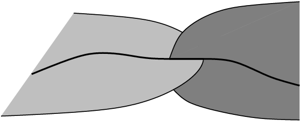
    for all i≠ji\neq j, Si∩SjS_{i}\cap S_{j} is either empty or a union of clasps (see Figure 1);

  3. (iii)

    for all i,j,ki,j,k pairwise distinct, Si∩Sj∩SkS_{i}\cap S_{j}\cap S_{k} is empty.

Refer to caption
Figure 1. A clasp intersection.

The existence of a C-complex for a colored link is fairly easy, see [4, Lemma 1]. In the case μ=1\mu=1, a C-complex for LL is nothing but a (possibly disconnected) Seifert surface for the link LL. Let us now define the corresponding generalization of the Seifert form. Let Ni=Si×[−1,1]N_{i}=S_{i}\times[-1,1] be a bicollar neighborhood of SiS_{i}. Given a sign εi=±1\varepsilon_{i}=\pm 1, let SiεiS_{i}^{\varepsilon_{i}} be the translated surface Si×{εi}⊂NiS_{i}\times\{\varepsilon_{i}\}\subset N_{i}. Also, let XX be the complement of an open tubular neighborhood of LL, and let YY be the complement of ⋃i=1μi​n​t​Ni\bigcup_{i=1}^{\mu}int\,N_{i} in XX. Given a sequence ε=(ε1,…,εμ)\varepsilon=(\varepsilon_{1},\dots,\varepsilon_{\mu}) of ±1\pm 1’s, set

Sε=⋃i=1μSiεi∩Y.S^{\varepsilon}=\bigcup_{i=1}^{\mu}S_{i}^{\varepsilon_{i}}\cap Y.

Since all the intersections are clasps, there is an obvious homotopy equivalence between SS and SεS^{\varepsilon} inducing an isomorphism H1​(S)→H1​(Sε)H_{1}(S)\to H_{1}(S^{\varepsilon}). Let iε:H1​(S)→H1​(S3∖S)i^{\varepsilon}\colon H_{1}(S)\to H_{1}(S^{3}\setminus S) be the composition of this isomorphism with the inclusion homomorphism H1​(Sε)→H1​(S3∖S)H_{1}(S^{\varepsilon})\to H_{1}(S^{3}\setminus S). Finally, let

αε:H1​(S)×H1​(S)→ℤ\alpha^{\varepsilon}\colon H_{1}(S)\times H_{1}(S)\to\mathbb{Z}

be the bilinear form given by αε​(x,y)=l​k​(iε​(x),y)\alpha^{\varepsilon}(x,y)=lk(i^{\varepsilon}(x),y), where l​klk denotes the linking number. Fix a basis of H1​(S)H_{1}(S) and denote by ASεA_{S}^{\varepsilon} (or simply by AεA^{\varepsilon}) the matrix of αε\alpha^{\varepsilon}. Of course, if μ=1\mu=1, then α−\alpha^{-} is the usual Seifert form and A−A^{-} the usual Seifert matrix. Note that for all ε\varepsilon, A−εA^{-\varepsilon} is equal to (Aε)T(A^{\varepsilon})^{T}, the transpose of the matrix AεA^{\varepsilon}.

For computational purposes, the following alternative definition of iεi^{\varepsilon} is more convenient. A 11-cycle in a C-complex is called a loop if it is an oriented simple closed curve which behaves as illustrated in Figure 2 whenever it crosses a clasp. Clearly, there exists a collection of loops whose homology classes form a basis of H1​(S)H_{1}(S). Therefore, it is possible to define iεi^{\varepsilon} as follows: for any loop xx, iε​([x])i^{\varepsilon}([x]) is the class of the 11-cycle obtained by pushing xx in the εi\varepsilon_{i}-normal direction off SiS_{i} for i=1,…,μi=1,\dots,\mu. The fact that xx is a loop ensures that this can be done continuously along the clasp intersections. We easily check that this definition of iεi^{\varepsilon} coincides with the intrinsic definition given above.
Refer to caption
Figure 2. A loop crossing a clasp.

2.2. The signature and nullity of a colored link

Let LL be a μ\mu-colored link. Consider a C-complex SS for LL and the associated Seifert matrices AεA^{\varepsilon} with respect to some fixed basis of H1​(S)H_{1}(S). Let A⁡(t1,…,tμ)A(t_{1},\dots,t_{\mu}) be the matrix with coefficients in ℤ⁡[t1,…,tμ]\mathbb{Z}[t_{1},\dots,t_{\mu}] defined by

A(t1,…,tμ)=∑εε1⋯εμt11−ε12⋯tμ1−εμ2Aε,A(t_{1},\dots,t_{\mu})=\sum_{\varepsilon}\,\varepsilon_{1}\cdots\varepsilon_{\mu}\,t_{1}^{\frac{1-\varepsilon_{1}}{2}}\cdots t_{\mu}^{\frac{1-\varepsilon_{\mu}}{2}}A^{\varepsilon},

where the sum is on the 2μ2^{\mu} possible sequences ε=(ε1,…,εμ)\varepsilon=(\varepsilon_{1},\dots,\varepsilon_{\mu}) of ±1\pm 1’s. For ω=(ω1,…,ωμ)\omega=(\omega_{1},\dots,\omega_{\mu}) in Tμ=S1×⋯×S1⊂ℂμT^{\mu}=S^{1}\times\dots\times S^{1}\subset\mathbb{C}^{\mu}, set

H⁡(ω)=∏i=1μ(1−ω¯i)​A​(ω1,…,ωμ).H(\omega)\;=\;\prod_{i=1}^{\mu}(1-\overline{\omega}_{i})\,A(\omega_{1},\dots,\omega_{\mu}).

Using the fact that A−ε=(Aε)TA^{-\varepsilon}=(A^{\varepsilon})^{T}, one easily checks that H⁡(ω)H(\omega) is a Hermitian matrix. Recall that the eigenvalues of such a matrix HH are real. Its signature sign​(H)\hbox{sign}\,(H) is defined as the number of positive eigenvalues minus the number of negative eigenvalues. The nullity null​(H)\hbox{null}\,(H) is the number of zero eigenvalues of HH.

Definition.

Let T∗μT^{\mu}_{\ast} be the open subset (S1∖{1})μ(S^{1}\setminus\{1\})^{\mu} of the μ\mu-dimensional torus Tμ⊂ℂμT^{\mu}\subset\mathbb{C}^{\mu}. The signature and nullity of the μ\mu-colored link LL are the functions

σL,ηL:T∗μ⟶ℤ\sigma_{L},\eta_{L}\colon T^{\mu}_{\ast}\longrightarrow\mathbb{Z}

given by σL​(ω)=sign​(H⁡(ω))\sigma_{L}(\omega)=\hbox{sign}\,(H(\omega)) and ηL​(ω)=null​(H⁡(ω))+β0​(S)−1\eta_{L}(\omega)=\hbox{null}\,(H(\omega))+\beta_{0}(S)-1, where β0​(S)\beta_{0}(S) denotes the number of connected components of SS.

By Sylvester’s theorem, σL​(ω)\sigma_{L}(\omega) and ηL​(ω)\eta_{L}(\omega) do not depend on the choice of a basis of H1​(S)H_{1}(S).

Theorem 2.1.

The signature σL\sigma_{L} and nullity ηL\eta_{L} do not depend on the choice of the C-complex for the colored link LL. Hence, they are well-defined as isotopy invariants of the colored link LL.

This theorem relies on the following lemma (see [4] for the proof).

Lemma 2.2.

Let SS and S′S^{\prime} be C-complexes for isotopic colored links. Then, SS and S′S^{\prime} can be transformed into each other by a finite number of the following operations and their inverses:

  • (T0)

    ambient isotopy;

  • (T1)

    handle attachment on one surface;

  • (T2)

    addition of a ribbon intersection, followed by a ‘push along an arc’ through this intersection (see Figure 3);

  • (T3)

    the transformation described in Figure 3.

Refer to caption
Figure 3. The transformations T​2T2 and T​3T3 in Lemma 2.2.
Proof of Theorem 2.1.

Let HH and H′H^{\prime} be two Hermitian matrices. We shall call H′H^{\prime} an elementary enlargement of HH if

H′=(Hξ0ξ¯Tλα0α¯0),H^{\prime}=\begin{pmatrix}H&\xi&0\cr\overline{\xi}^{T}&\lambda&\alpha\cr 0&\overline{\alpha}&0\end{pmatrix},

where ξ\xi is any complex vector, λ\lambda any real number and α∈ℂ∗\alpha\in\mathbb{C}^{\ast}. HH is called an elementary reduction of H′H^{\prime}. One easily checks that the signature and nullity of a Hermitian matrix are unchanged by elementary enlargements and reductions. By Lemma 2.2, it remains to prove that the transformations T​1T1 to T​3T3 of a C-complex induce finite sequences of elementary reductions and enlargements on the corresponding Hermitian matrices (or other elementary transformations leaving the signature and nullity unchanged).

(T​1)(T1) Let S′S^{\prime} be a C-complex obtained from a C-complex SS by a handle attachment on SkS_{k}. If this handle connects two distinct connected components of SS, then H1​(S′)=H1​(S)⊕ℤ​yH_{1}(S^{\prime})=H_{1}(S)\oplus\mathbb{Z}y, where yy in a 11-cycle such that l​k​(iε​(y),z)=0lk(i^{\varepsilon}(y),z)=0 for all zz in H1​(S′)H_{1}(S^{\prime}). Hence, the Hermitian matrices HH and H′H^{\prime} corresponding to SS and S′S^{\prime} are related by H′=H⊕(0)H^{\prime}=H\oplus(0), so sign​(H′)=sign​(H)\hbox{sign}\,(H^{\prime})=\hbox{sign}\,(H) and null​(H′)=null​(H)+1\hbox{null}\,(H^{\prime})=\hbox{null}\,(H)+1. Since β0​(S′)=β0​(S)−1\beta_{0}(S^{\prime})=\beta_{0}(S)-1, the signature and nullity of LL are unchanged. Let us now assume that this handle attachement is performed on one connected component of SS. In this case, H1​(S′)=H1​(S)⊕ℤ​x⊕ℤ​yH_{1}(S^{\prime})=H_{1}(S)\oplus\mathbb{Z}x\oplus\mathbb{Z}y. Moreover, the cycles xx and yy can be chosen so that the corresponding Seifert matrices satisfy

AS′ε=(ASε∗0∗∗π⁡(−ε)0π⁡(ε)0),withπ⁡(ε)={1if εk=+1;0else.A_{S^{\prime}}^{\varepsilon}=\begin{pmatrix}A_{S}^{\varepsilon}&\ast&0\cr\ast&\ast&\pi(-\varepsilon)\cr 0&\pi(\varepsilon)&0\end{pmatrix}\,,\quad\hbox{with}\quad\pi(\varepsilon)=\begin{cases}1&\text{if $\varepsilon_{k}=+1$;}\cr 0&\text{else.}\end{cases}

Such a choice of xx and yy is illustrated below.

[Uncaptioned image]

This time, the Hermitian matrices HH and H′H^{\prime} are related by

H′​(ω)=(H⁡(ω)∗0∗∗α0α¯0),H^{\prime}(\omega)=\begin{pmatrix}H(\omega)&\ast&0\cr\ast&\ast&\alpha\cr 0&\overline{\alpha}&0\end{pmatrix},

with α=(1−ω¯k)​∏i≠k|1−ωi|2\alpha=(1-\overline{\omega}_{k})\prod_{i\neq k}|1-\omega_{i}|^{2}. Since H′​(ω)H^{\prime}(\omega) is Hermitian and ωi≠1\omega_{i}\neq 1 for all ii, H′​(ω)H^{\prime}(\omega) is an elementary enlargement of H⁡(ω)H(\omega).

(T​2)(T2) Let S′S^{\prime} be a C-complex obtained from SS by the transformation T​2T2. If this transformation connects two distinct connected components of SS, then H1​(S′)=H1​(S)⊕ℤ​zH_{1}(S^{\prime})=H_{1}(S)\oplus\mathbb{Z}z. As above, we get H′=H⊕(0)H^{\prime}=H\oplus(0) and β0​(S′)=β0​(S)−1\beta_{0}(S^{\prime})=\beta_{0}(S)-1, so the signature and nullity are unchanged. On the other hand, if this transformation take place on one connected component of SS, then H1​(S′)=H1​(S)⊕ℤ​w⊕ℤ​zH_{1}(S^{\prime})=H_{1}(S)\oplus\mathbb{Z}w\oplus\mathbb{Z}z with ww and zz as illustrated below.

[Uncaptioned image]

Therefore,

AS′ε=(ASε∗0∗∗δ⁡(−ε)0δ⁡(ε)0),withδ⁡(ε)={1if εj=εk=+1;0else.A_{S^{\prime}}^{\varepsilon}=\begin{pmatrix}A_{S}^{\varepsilon}&\ast&0\cr\ast&\ast&\delta(-\varepsilon)\cr 0&\delta(\varepsilon)&0\end{pmatrix}\,,\quad\hbox{with}\quad\delta(\varepsilon)=\begin{cases}1&\text{if $\varepsilon_{j}=\varepsilon_{k}=+1$;}\cr 0&\text{else.}\end{cases}

It follows that the corresponding Hermitian matrix H′​(ω)H^{\prime}(\omega) is an elementary enlargement of H⁡(ω)H(\omega) with α=(1−ω¯j)​(1−ω¯k)​∏i≠j,k|1−ωi|2\alpha=(1-\overline{\omega}_{j})(1-\overline{\omega}_{k})\prod_{i\neq j,k}|1-\omega_{i}|^{2}.

(T​3)(T3) Finally, let SS and S′S^{\prime} be C-complexes related by the move T​3T3. A similar computation shows that the corresponding Hermitian matrices H⁡(ω)H(\omega) and H′​(ω)H^{\prime}(\omega) are both an elementary enlargement of some Hermitian matrix. This concludes the proof. ∎

Example 2.3.

If μ=1\mu=1, then the colored link LL is just a link. Furthermore, a C-complex SS for LL is nothing but a (possibly disconnected) Seifert surface for LL. Finally, A−A^{-} is a usual Seifert matrix AA, and A+=ATA^{+}=A^{T}. Hence, the corresponding Hermitian matrix is given by

H⁡(ω)=(1−ω¯)​(AT−ω​A)=(1−ω)​A+(1−ω¯)​AT.H(\omega)=(1-\overline{\omega})(A^{T}-\omega A)=(1-\omega)A+(1-\overline{\omega})A^{T}.

So if μ=1\mu=1, the signature of LL is the Levine-Tristram signature of the link LL.

[Uncaptioned image]
Example 2.4.

Consider the 22-colored link LL illustrated above. A C-complex SS for LL is also given. We compute Aε=(−1)A^{\varepsilon}=(-1) if ε1=ε2\varepsilon_{1}=\varepsilon_{2}, and Aε=(0)A^{\varepsilon}=(0) else. Hence,

H⁡(ω1,ω2)=(1−ω¯1)​(1−ω¯2)​(−1−ω1​ω2)=−2​ℜ⁡((1−ω1)​(1−ω2)).H(\omega_{1},\omega_{2})=(1-\overline{\omega}_{1})(1-\overline{\omega}_{2})(-1-\omega_{1}\omega_{2})=-2\Re((1-\omega_{1})(1-\omega_{2})).

So σL​(ω1,ω2)\sigma_{L}(\omega_{1},\omega_{2}) is given by the sign of −ℜ⁡((1−ω1)​(1−ω2))-\Re((1-\omega_{1})(1-\omega_{2})). Furthermore, ηL​(ω1,ω2)=1\eta_{L}(\omega_{1},\omega_{2})=1 if ω1​ω2=−1\omega_{1}\omega_{2}=-1, and ηL​(ω1,ω2)=0\eta_{L}(\omega_{1},\omega_{2})=0 else. Let us draw the domain T∗2T_{\ast}^{2} as a square. The value of the function σL\sigma_{L} can be represented as illustrated opposite. Note that σL\sigma_{L} and ηL\eta_{L} are constant on the connected components of the complement of the zeroes of ΔL​(t1,t2)=t1​t2+1\Delta_{L}(t_{1},t_{2})=t_{1}t_{2}+1, the Alexander polynomial of LL. We shall explain this fact in Section 4.

[Uncaptioned image]
Proposition 2.5.

Let L=L1∪⋯∪Lμ+1L=L_{1}\cup\dots\cup L_{\mu+1} be a (μ+1)(\mu+1)-colored link. Consider the μ\mu-colored link L′=L1′∪⋯∪Lμ′L^{\prime}=L^{\prime}_{1}\cup\dots\cup L^{\prime}_{\mu} given by Li′=LiL^{\prime}_{i}=L_{i} for i<μi<\mu and Lμ′=Lμ∪Lμ+1L^{\prime}_{\mu}=L_{\mu}\cup L_{\mu+1}. Then, for all (ω1,…,ωμ)(\omega_{1},\dots,\omega_{\mu}) in T∗μT^{\mu}_{*},

σL′​(ω1,…,ωμ)\displaystyle\sigma_{L^{\prime}}(\omega_{1},\dots,\omega_{\mu}) =\displaystyle= σL​(ω1,…,ωμ,ωμ)−l​k​(Lμ,Lμ+1),\displaystyle\sigma_{L}(\omega_{1},\dots,\omega_{\mu},\omega_{\mu})-lk(L_{\mu},L_{\mu+1}),
ηL′​(ω1,…,ωμ)\displaystyle\eta_{L^{\prime}}(\omega_{1},\dots,\omega_{\mu}) =\displaystyle= ηL​(ω1,…,ωμ,ωμ).\displaystyle\eta_{L}(\omega_{1},\dots,\omega_{\mu},\omega_{\mu}).

Before giving the proof of this proposition, let us point out an interesting consequence: it is possible to compute the signature and nullity of a μ\mu-colored link by considering any finer coloring of the same underlying link. In particular, all the signatures (corresponding to all the possible colorings) can be computed from the signature corresponding to a coloring with the maximal number of colors. This simplifies greatly the computations in many cases, as illustrated by the following (didactic) example.

Example 2.6.

Let us try to compute the Levine-Tristram signature of the link LL illustrated below. One possibility is to choose a Seifert surface for LL and to compute the corresponding Seifert matrix.

On the other hand, consider a 33-colored link L′L^{\prime} obtained by coloring the components of LL with three different colors. There is an obvious contractible C-complex for L′L^{\prime}, so σL′\sigma_{L^{\prime}} is identically zero. By Proposition 2.5, the Levine-Tristram signature of LL is given by σL​(ω)=σL′​(ω,ω,ω)−2=−2\sigma_{L}(\omega)=\sigma_{L^{\prime}}(\omega,\omega,\omega)-2=-2.

[Uncaptioned image]
Proof of Proposition 2.5.

First, note that it is sufficient to prove this statement when Lμ+1L_{\mu+1} is a knot. Consider a C-complex S=S1∪⋯∪Sμ+1S=S_{1}\cup\dots\cup S_{\mu+1} for LL, and let ℓ\ell be the number of clasps in Sμ∩Sμ+1S_{\mu}\cap S_{\mu+1}. A certain number of these clasps (say, ℓ+\ell_{+}) induce a positive linking number between LμL_{\mu} and Lμ+1L_{\mu+1}, while the ℓ−\ell_{-} remaining ones induce a negative linking number. By definition, ℓ=ℓ++ℓ−\ell=\ell_{+}+\ell_{-} and l​k​(Lμ,Lμ+1)=ℓ+−ℓ−lk(L_{\mu},L_{\mu+1})=\ell_{+}-\ell_{-}. Using transformation T​2T2 of Figure 3, it may be assumed that ℓ+\ell_{+} and ℓ−\ell_{-} are positive. Via handle attachment, it may also be assumed that SμS_{\mu} is connected. Finally, one easily checks that the C-complex SS can be chosen so that the knot Lμ+1L_{\mu+1} crosses the ℓ−\ell_{-} negative clasps first, and then the ℓ+\ell_{+} positive ones. This situation is illustrated below.

[Uncaptioned image]

Let S~\widetilde{S} be the C-complex obtained from SS by removing these ℓ\ell clasps. Since SμS_{\mu} and Sμ+1S_{\mu+1} are connected, H1​(S)=⨁i=1ℓ−1ℤ​xi⊕H1​(S~)H_{1}(S)=\bigoplus_{i=1}^{\ell-1}\mathbb{Z}x_{i}\oplus H_{1}(\widetilde{S}), with xix_{i} the 11-cycles in Sμ∪Sμ+1S_{\mu}\cup S_{\mu+1} depicted above. Fix a basis ℬ\mathcal{B} of H1​(S~)H_{1}(\widetilde{S}). For any sequence ε=(ε1,…,εμ+1)\varepsilon=(\varepsilon_{1},\dots,\varepsilon_{\mu+1}) of ±1\pm 1’s, the Seifert matrix ASεA_{S}^{\varepsilon} corresponding to the basis ⟨x1,…,xℓ−1⟩∪ℬ\left<x_{1},\dots,x_{\ell-1}\right>\cup{\mathcal{B}} of H1​(S)H_{1}(S) can be written

ASε=(Dεμ​εμ+1Cεμ(C−εμ)TAS~ε).A_{S}^{\varepsilon}=\begin{pmatrix}D^{\varepsilon_{\mu}\varepsilon_{\mu+1}}&C^{\varepsilon_{\mu}}\cr(C^{-\varepsilon_{\mu}})^{T}&A_{\widetilde{S}}^{\varepsilon}\end{pmatrix}.

Fix an element ω′=(ω1,…,ωμ)\omega^{\prime}=(\omega_{1},\dots,\omega_{\mu}) of T∗μT^{\mu}_{*}. Since Dεμ​εμ+1D^{\varepsilon_{\mu}\varepsilon_{{\mu+1}}} only depends on εμ\varepsilon_{\mu} and εμ+1\varepsilon_{{\mu+1}}, the upper left block of the corresponding Hermitian matrix HS​(ω′,ωμ)H_{S}(\omega^{\prime},\omega_{\mu}) is given by

∏i=1μ|1−ωi|2​(λ​D+λ¯​DT+N),\prod_{i=1}^{\mu}|1-\omega_{i}|^{2}(\lambda D+\overline{\lambda}D^{T}+N),

where λ=1−ωμ\lambda=1-\omega_{\mu}, D=D−⁣−D=D^{--} and

(⋆) N=(D−⁣+−D)+(D−⁣+−D)T=(−211⋱⋱⋱−2110−1−12⋱⋱⋱−1−12).N=(D^{-+}-D)+(D^{-+}-D)^{T}=\begin{pmatrix}-2&1\cr\phantom{-}1&\ddots&\ddots\cr&\ddots&-2&\!\!\phantom{-}1\cr&&\phantom{-}1&\!\!\phantom{-}0&-1\cr&&&\!\!-1&\phantom{-}2&\ddots\cr&&&&\ddots&\ddots&-1\cr&&&&&-1&\phantom{-}2\end{pmatrix}.

Similarly, the upper right block of HS​(ω′,ωμ)H_{S}(\omega^{\prime},\omega_{\mu}) is equal to ∏i=1μ|1−ωi|2​(λ​C−+λ¯​C+)\prod_{i=1}^{\mu}|1-\omega_{i}|^{2}(\lambda C^{-}+\overline{\lambda}C^{+}). Finally, observe that each coefficient of AS~εA_{\widetilde{S}}^{\varepsilon} is either independant of εμ\varepsilon_{\mu}, or independant of εμ+1\varepsilon_{\mu+1}. Therefore, HS~​(ω′,ωμ)=|λ|2​HS~′​(ω′)H_{\widetilde{S}}(\omega^{\prime},\omega_{\mu})=|\lambda|^{2}H_{\widetilde{S}^{\prime}}(\omega^{\prime}), where S~′=S1∪⋯∪Sμ−1∪S~μ′\widetilde{S}^{\prime}=S_{1}\cup\dots\cup S_{\mu-1}\cup\widetilde{S}_{\mu}^{\prime} and S~μ′=S~μ⊔S~μ+1\widetilde{S}_{\mu}^{\prime}=\widetilde{S}_{\mu}\sqcup\widetilde{S}_{\mu+1}. To sum up, we have the equality

(⋆⋆) HS​(ω′,ωμ)=∏i=1μ|1−ωi|2​(λ​D+λ¯​DT+Nλ​C−+λ¯​C+(λ¯​C−+λ​C+)T∏i=1μ−1|1−ωi|−2​HS~′​(ω′)).H_{S}(\omega^{\prime},\omega_{\mu})=\prod_{i=1}^{\mu}|1-\omega_{i}|^{2}\begin{pmatrix}\lambda D+\overline{\lambda}D^{T}+N&\lambda C^{-}+\overline{\lambda}C^{+}\cr(\overline{\lambda}C^{-}+\lambda C^{+})^{T}&\prod_{i=1}^{\mu-1}|1-\omega_{i}|^{-2}H_{\widetilde{S}^{\prime}}(\omega^{\prime})\end{pmatrix}.

Let us now turn to the μ\mu-colored link L′L^{\prime}. The C-complex SS can be transformed into a C-complex S′=S1′∪⋯∪Sμ′S^{\prime}=S_{1}^{\prime}\cup\dots\cup S^{\prime}_{\mu} for L′L^{\prime} as follows: set Si′=SiS_{i}^{\prime}=S_{i} for i<μi<\mu, and let Sμ′S^{\prime}_{\mu} be the surface obtained from Sμ∪Sμ+1S_{\mu}\cup S_{\mu+1} by ‘smoothing’ the ℓ\ell clasps as illustrated below.

[Uncaptioned image]

Basically, each clasp is replaced by two half-twisted bands joining SμS_{\mu} and Sμ+1S_{\mu+1}. This time, H1​(S′)=⨁i=1ℓℤ​yi⊕⨁i=1ℓ−1ℤ​xi′⊕H1​(S~′)H_{1}(S^{\prime})=\bigoplus_{i=1}^{\ell}\mathbb{Z}y_{i}\oplus\bigoplus_{i=1}^{\ell-1}\mathbb{Z}x^{\prime}_{i}\oplus H_{1}(\widetilde{S}^{\prime}) with the 11-cycles yiy_{i} and xi′x_{i}^{\prime} depicted above. Using the same method and notations as above, one can compute the Hermitian matrix HS′​(ω′)H_{S^{\prime}}(\omega^{\prime}) corresponding to the basis ⟨y1,…,yℓ,x1′​…,xℓ−1′⟩∪ℬ\left<y_{1},\dots,y_{\ell},x_{1}^{\prime}\dots,x_{\ell-1}^{\prime}\right>\cup{\mathcal{B}} of H1​(S′)H_{1}(S^{\prime}). It is given by

∏i=1μ|1−ωi|2​(|λ|2​(Iℓ−⊕−Iℓ+)λ¯​M0λ​MTλ​D+λ¯​DTλ​C−+λ¯​C+0(λ¯​C−+λ​C+)T∏i=1μ−1|1−ωi|−2​HS~′​(ω′)),\prod_{i=1}^{\mu}|1-\omega_{i}|^{2}\begin{pmatrix}|\lambda|^{2}(I_{\ell_{-}}\oplus-I_{\ell_{+}})&\overline{\lambda}M&0\cr\lambda M^{T}&\lambda D+\overline{\lambda}D^{T}&\lambda C^{-}+\overline{\lambda}C^{+}\cr 0&(\overline{\lambda}C^{-}+\lambda C^{+})^{T}&\prod_{i=1}^{\mu-1}|1-\omega_{i}|^{-2}H_{\widetilde{S}^{\prime}}(\omega^{\prime})\end{pmatrix},

where IkI_{k} denotes the (k×k)(k\times k)-identity matrix and

M=(1−1⋱⋱1−1).M=\begin{pmatrix}\phantom{-}1\cr-1&\ddots\cr&\ddots&\!\!\phantom{-}1\cr&&\!\!-1\end{pmatrix}.

Using the equalities (⋆)(\star) and (⋆⋆)(\star\star) together with the fact that λ≠0\lambda\neq 0, it is easy to check that the matrix HS′​(ω′)H_{S^{\prime}}(\omega^{\prime}) is conjugate to the Hermitian matrix Iℓ−⊕−Iℓ+⊕HS​(ω′,ωμ)I_{\ell_{-}}\oplus-I_{\ell_{+}}\oplus H_{S}(\omega^{\prime},\omega_{\mu}). Hence,

σL′​(ω′)\displaystyle\sigma_{L^{\prime}}(\omega^{\prime}) =\displaystyle= sign​(HS′​(ω′))=sign​(HS​(ω′,ωμ))+ℓ−−ℓ+\displaystyle\hbox{sign}\,(H_{S^{\prime}}(\omega^{\prime}))=\hbox{sign}\,(H_{S}(\omega^{\prime},\omega_{\mu}))+\ell_{-}-\ell_{+}
=\displaystyle= σL​(ω′,ωμ)−l​k​(Lμ,Lμ+1),\displaystyle\sigma_{L}(\omega^{\prime},\omega_{\mu})-lk(L_{\mu},L_{\mu+1}),

and null​HS′​(ω′)=null​HS​(ω′,ωμ)\hbox{null}\,H_{S^{\prime}}(\omega^{\prime})=\hbox{null}\,H_{S}(\omega^{\prime},\omega_{\mu}). Since β0​(S)=β0​(S′)\beta_{0}(S)=\beta_{0}(S^{\prime}), the proposition is proved. ∎

Note that we shall give an alternative proof of this result in subsection 6.3.

2.3. Basic properties of σL\sigma_{L} and ηL\eta_{L}

We conclude this section with an enumeration of several properties of the signature and nullity. Deeper properties shall be presented in the following sections. The first proposition follows easily from the fact that H⁡(ω)H(\omega) is Hermitian.

Proposition 2.7.

For any (ω1,…,ωμ)∈T∗μ(\omega_{1},\dots,\omega_{\mu})\in T_{\ast}^{\mu},

σL​(ω1−1,…,ωμ−1)\displaystyle\sigma_{L}(\omega^{-1}_{1},\dots,\omega^{-1}_{\mu}) =\displaystyle= σL​(ω1,…,ωμ),\displaystyle\sigma_{L}(\omega_{1},\dots,\omega_{\mu}),
ηL​(ω1−1,…,ωμ−1)\displaystyle\eta_{L}(\omega^{-1}_{1},\dots,\omega^{-1}_{\mu}) =\displaystyle= ηL​(ω1,…,ωμ).∎\displaystyle\eta_{L}(\omega_{1},\dots,\omega_{\mu}).\qed
Proposition 2.8.

Let LL be a colored link, and let L′L^{\prime} be the colored link obtained from LL by reversing the orientation of every component of the sublink L1L_{1} of LL. Then, for all ω=(ω1,…,ωμ)\omega=(\omega_{1},\dots,\omega_{\mu}) in T∗μT^{\mu}_{\ast},

σL′​(ω1,…,ωμ)\displaystyle\sigma_{L^{\prime}}(\omega_{1},\dots,\omega_{\mu}) =\displaystyle= σL​(ω1−1,ω2,…,ωμ),\displaystyle\sigma_{L}(\omega^{-1}_{1},\omega_{2},\dots,\omega_{\mu}),
ηL′​(ω1,…,ωμ)\displaystyle\eta_{L^{\prime}}(\omega_{1},\dots,\omega_{\mu}) =\displaystyle= ηL​(ω1−1,ω2,…,ωμ).\displaystyle\eta_{L}(\omega_{1}^{-1},\omega_{2},\dots,\omega_{\mu}).
Proof.

If S=S1∪S2∪⋯∪SμS=S_{1}\cup S_{2}\cup\dots\cup S_{\mu} is a C-complex for LL, then S′=(−S1)∪S2∪⋯∪SμS^{\prime}=(-S_{1})\cup S_{2}\cup\dots\cup S_{\mu} is a C-complex for L′L^{\prime}. Since AS′ε′=ASεA_{S^{\prime}}^{\varepsilon^{\prime}}=A_{S}^{\varepsilon} with ε1′=−ε1\varepsilon_{1}^{\prime}=-\varepsilon_{1} and εi′=εi\varepsilon^{\prime}_{i}=\varepsilon_{i} for i>1i>1, the corresponding Hermitian matrices H′H^{\prime} and HH are related by H′​(ω1,ω2,…,ωμ)=H⁡(ω1−1,ω2,…,ωμ)H^{\prime}(\omega_{1},\omega_{2},\dots,\omega_{\mu})=H(\omega^{-1}_{1},\omega_{2},\dots,\omega_{\mu}). ∎

Corollary 2.9.

If −L-L denotes the colored link LL with the opposite orientation, then σ−L=σL\sigma_{-L}=\sigma_{L} and η−L=ηL\eta_{-L}=\eta_{L}.∎

So the signature cannot distinguish between a colored link and its inverse. On the other hand, it is a useful invariant for telling apart a colored link and its mirror image.

Proposition 2.10.

If L¯\overline{L} denotes the mirror image of the colored link LL, then σL¯=−σL\sigma_{\overline{L}}=-\sigma_{L} and ηL¯=ηL\eta_{\overline{L}}=\eta_{L}.

Proof.

If SS is a C-complex for LL, then the mirror image S′S^{\prime} of SS is a C-complex for L¯\overline{L}. Therefore, AS′ε=−ASεA_{S^{\prime}}^{\varepsilon}=-A_{S}^{\varepsilon} and the Hermitian matrices HH and H′H^{\prime} satisfy H′​(ω)=−H⁡(ω)H^{\prime}(\omega)=-H(\omega). ∎

Corollary 2.11.

If a colored link LL is isotopic to its mirror image, then σL\sigma_{L} is identically zero.∎

Finally, the signature and nullity behave well under connected and disjoint sum.

Proposition 2.12.

Let L′=L1∪⋯∪Lν−1∪Lν′L^{\prime}=L_{1}\cup\dots\cup L_{\nu-1}\cup L^{\prime}_{\nu} and L′′=Lν′′∪Lν+1∪⋯∪LμL^{\prime\prime}=L^{\prime\prime}_{\nu}\cup L_{\nu+1}\cup\dots\cup L_{\mu} be two colored links. Consider a colored link L=L1∪⋯∪LμL=L_{1}\cup\dots\cup L_{\mu}, where LνL_{\nu} is a connected sum of Lν′L^{\prime}_{\nu} and Lν′′L^{\prime\prime}_{\nu} along any of their components. Then, for all ω1,…,ωμ∈S1∖{1}\omega_{1},\dots,\omega_{\mu}\in S^{1}\setminus\{1\},

σL​(ω1,…,ωμ)\displaystyle\sigma_{L}(\omega_{1},\dots,\omega_{\mu}) =\displaystyle= σL′​(ω1,…,ων)+σL′′​(ων,…,ωμ),\displaystyle\sigma_{L^{\prime}}(\omega_{1},\dots,\omega_{\nu})+\sigma_{L^{\prime\prime}}(\omega_{\nu},\dots,\omega_{\mu}),
ηL​(ω1,…,ωμ)\displaystyle\eta_{L}(\omega_{1},\dots,\omega_{\mu}) =\displaystyle= ηL′​(ω1,…,ων)+ηL′′​(ων,…,ωμ).\displaystyle\eta_{L^{\prime}}(\omega_{1},\dots,\omega_{\nu})+\eta_{L^{\prime\prime}}(\omega_{\nu},\dots,\omega_{\mu}).
Proof.

Given S′S^{\prime} a C-complex for L′L^{\prime} and S′′S^{\prime\prime} a C-complex for L′′L^{\prime\prime}, a C-complex SS for LL is given by the band sum of S′S^{\prime} and S′′S^{\prime\prime} along the corresponding components of Sν′S^{\prime}_{\nu} and Sν′′S^{\prime\prime}_{\nu}. Since S′S^{\prime} and S′′S^{\prime\prime} have no closed components, this band can be chosen such that only its ends meet S′S^{\prime} and S′′S^{\prime\prime}. Clearly, ASε=AS′ε′⊕AS′′ε′′A^{\varepsilon}_{S}=A_{S^{\prime}}^{\varepsilon^{\prime}}\oplus A_{S^{\prime\prime}}^{\varepsilon^{\prime\prime}} with ε′=(ε1,…,εν)\varepsilon^{\prime}=(\varepsilon_{1},\dots,\varepsilon_{\nu}) and ε′′=(εν,…,εμ)\varepsilon^{\prime\prime}=(\varepsilon_{\nu},\dots,\varepsilon_{\mu}). The corresponding Hermitian matrices HH, H′H^{\prime} and H′′H^{\prime\prime} satisfy

H⁡(ω1,…,ωμ)=∏i>ν|1−ωi|2​H′​(ω1,…,ων)⊕∏i<ν|1−ωi|2​H′′​(ων,…,ωμ).H(\omega_{1},\dots,\omega_{\mu})=\prod_{i>\nu}|1-\omega_{i}|^{2}H^{\prime}(\omega_{1},\dots,\omega_{\nu})\oplus\prod_{i<\nu}|1-\omega_{i}|^{2}H^{\prime\prime}(\omega_{\nu},\dots,\omega_{\mu}).

Since ωi≠1\omega_{i}\neq 1 for all ii and β0​(S)=β0​(S′)+β0​(S′′)−1\beta_{0}(S)=\beta_{0}(S^{\prime})+\beta_{0}(S^{\prime\prime})-1, this implies the proposition. ∎

Proposition 2.13.

Let L′L^{\prime} and L′′L^{\prime\prime} be colored links with disjoint sets of colors. Consider the colored link LL given by the disjoint sum of L′L^{\prime} and L′′L^{\prime\prime}. Then,

σL​(ω′,ω′′)\displaystyle\sigma_{L}(\omega^{\prime},\omega^{\prime\prime}) =\displaystyle= σL′​(ω′)+σL′′​(ω′′),\displaystyle\sigma_{L^{\prime}}(\omega^{\prime})+\sigma_{L^{\prime\prime}}(\omega^{\prime\prime}),
ηL​(ω′,ω′′)\displaystyle\eta_{L}(\omega^{\prime},\omega^{\prime\prime}) =\displaystyle= ηL′​(ω′)+ηL′′​(ω′′)+1.\displaystyle\eta_{L^{\prime}}(\omega^{\prime})+\eta_{L^{\prime\prime}}(\omega^{\prime\prime})+1.
Proof.

Let S′S^{\prime} and S′′S^{\prime\prime} be C-complexes for L′L^{\prime} and L′′L^{\prime\prime}. A C-complex SS for LL is given by the disjoint union of S′S^{\prime} and S′′S^{\prime\prime}. Clearly, AS(ε′,ε′′)=AS′ε′⊕AS′′ε′′A_{S}^{(\varepsilon^{\prime},\varepsilon^{\prime\prime})}=A_{S^{\prime}}^{\varepsilon^{\prime}}\oplus A_{S^{\prime\prime}}^{\varepsilon^{\prime\prime}}, so

H⁡(ω′,ω′′)=∏i|1−ωi′′|2​H′​(ω′)⊕∏j|1−ωj′|2​H′′​(ω′′).H(\omega^{\prime},\omega^{\prime\prime})=\prod_{i}|1-\omega^{\prime\prime}_{i}|^{2}H^{\prime}(\omega^{\prime})\oplus\prod_{j}|1-\omega^{\prime}_{j}|^{2}H^{\prime\prime}(\omega^{\prime\prime}).

Since β0​(S)=β0​(S′)+β0​(S′′)\beta_{0}(S)=\beta_{0}(S^{\prime})+\beta_{0}(S^{\prime\prime}), the proposition is proved. ∎

3. The Alexander module of a colored link

Associated to a μ\mu-colored link LL with exterior XX is a natural ℤμ\mathbb{Z}^{\mu}-covering X~→X\widetilde{X}\to X. The aim of this section is to show how the space X~\widetilde{X} can be constructed from a C-complex for LL. This leads to a presentation of the Alexander module of LL, that is, the ℤ⁡[t1±1,…,tμ±1]\mathbb{Z}[t_{1}^{\pm 1},\dots,t_{\mu}^{\pm 1}]-module H1​(X~)H_{1}(\widetilde{X}). This generalizes a celebrated theorem of Seifert, which corresponds to the case μ=1\mu=1.

We shall use these results in the next section to derive relations between the signature, the nullity, and the Alexander invariants of colored links.

3.1. Basics

Let L=L1∪⋯∪LμL=L_{1}\cup\dots\cup L_{\mu} be a colored link, and let XX denote its exterior. The epimorphism π1​(X)→ℤμ\pi_{1}(X)\to\mathbb{Z}^{\mu} given by γ↦(l​k​(γ,L1),…,l​k​(γ,Lμ))\gamma\mapsto(lk(\gamma,L_{1}),\dots,lk(\gamma,L_{\mu})) induces a regular ℤμ\mathbb{Z}^{\mu}-covering X~→X\widetilde{X}\to X. The homology of X~\widetilde{X} is a natural module over the ring Λμ=ℤ⁡[t1±1,…,tμ±1]\Lambda_{\mu}=\mathbb{Z}[t_{1}^{\pm 1},\dots,t_{\mu}^{\pm 1}], where tit_{i} denotes the covering transformation corresponding to an oriented meridian of LiL_{i}. The Λμ\Lambda_{\mu}-module H1​(X~)H_{1}(\widetilde{X}) is called the Alexander module of the colored link LL. Of course, if μ=1\mu=1, then H1​(X~)H_{1}(\widetilde{X}) is nothing but the usual Alexander module of the link LL.

To extract handy information from such a cumbersome invariant as a module over Λμ\Lambda_{\mu}, the standard trick is to consider its elementary ideals. Although these objects are widely used, their definitions vary according to the authors. Therefore, we shall now clarify the meaning of these concepts in the present work. Let RR be a noetherian factorial domain, that is, an integral domain in which every ideal is finitely generated, and every non-zero non-invertible element has a unique factorization. Let PP be an m×nm\times n matrix with coefficients in RR. Let us denote by Er​(P)E_{r}(P) the ideal of RR generated by all the (m−r)×(m−r)(m-r)\times(m-r) minors of PP. By convention, Er​(P)=(0)E_{r}(P)=(0) if r<0r<0 and Er​(P)=RE_{r}(P)=R if r≥mr\geq m. Let Δr​(P)\Delta_{r}(P) denote the greatest common divisor of the elements of Er​(P)E_{r}(P). (Recall that the greatest common divisor of a1,…,ana_{1},\dots,a_{n} in RR is an element dd of RR which divides aia_{i} for all ii, and such that if c∈Rc\in R divides aia_{i} for all ii, then cc divides dd.) Since RR is a noetherian factorial domain, Δr​(P)\Delta_{r}(P) exists, and is well-defined up to multiplication by a unit of RR. Given Δ\Delta and Δ′\Delta^{\prime} in RR, let us note Δ​=˙​Δ′\Delta\,\dot{=}\,\Delta^{\prime}\, if Δ=u​Δ′\,\Delta=u\Delta^{\prime} for some unit uu of RR. Now, let MM be a module over a factorial ring RR. A finite presentation of MM is an exact sequence F→φE→M→0F\stackrel{{\scriptstyle\varphi}}{{\to}}E\to M\to 0, where EE and FF are free RR-modules with finite basis. A matrix of φ\varphi is a presentation matrix of MM. The rt​hr^{th} elementary ideal of MM is the ideal of RR given by Er​(M):=Er​(P)E_{r}(M):=E_{r}(P), where PP is any presentation matrix of MM. It is easy to check that these ideals do not depend on the presentation of MM. In particular, the element Δr​(M):=Δr​(P)\Delta_{r}(M):=\Delta_{r}(P) of RR is well defined up to multiplication by a unit of RR.

Let us now turn back to colored links. Given a μ\mu-colored link LL, we just defined the Alexander module of LL as some module H1​(X~)H_{1}(\widetilde{X}) over the ring Λμ\Lambda_{\mu}. The rthr^{\mathrm{th}} elementary ideal Er​(H1​(X~))E_{r}(H_{1}(\widetilde{X})) is the rt​hr^{th} Alexander ideal of LL, and is denoted by Er​(L)E_{r}(L). The polynomial Δr​(L):=Δr​(H1​(X~))\Delta_{r}(L):=\Delta_{r}(H_{1}(\widetilde{X})) is called the rt​hr^{th} Alexander polynomial of LL; Δ0​(L)\Delta_{0}(L) is called the Alexander polynomial of LL, and is denoted by ΔL\Delta_{L}. Again, note that Δr​(L)\Delta_{r}(L) is only defined up to multiplication by a unit of Λμ\Lambda_{\mu}, that is, by ±t1m1⋯tμmμ\pm t_{1}^{m_{1}}\cdots t_{\mu}^{m_{\mu}} with integers mim_{i}.

3.2. A presentation of the Alexander module using a C-complex

Fix a colored link L=L1∪⋯∪LμL=L_{1}\cup\dots\cup L_{\mu}. Consider a C-complex S=S1∪⋯∪SμS=S_{1}\cup\dots\cup S_{\mu} for LL such that each SiS_{i} is connected and Si∩Sj≠∅S_{i}\cap S_{j}\neq\emptyset for all i≠ji\neq j. (Such a C-complex exists by transformations T​1T1 and T​2T2 of Lemma 2.2.) For i=1,…,μi=1,\dots,\mu, choose some interior point viv_{i} of Si∖⋃j≠iSi∩SjS_{i}\setminus\bigcup_{j\neq i}S_{i}\cap S_{j}. Given a clasp in Si∩SjS_{i}\cap S_{j} with i<ji<j, consider an oriented edge in Si∪SjS_{i}\cup S_{j} joining viv_{i} and vjv_{j} and passing through this single clasp as described in Figure 2. This leads to a collection of oriented edges {ei​j1,…,ei​jc⁡(i,j)}\{e_{ij}^{1},\dots,e_{ij}^{c(i,j)}\}, where c⁡(i,j)c(i,j) denotes the number of clasps in Si∩SjS_{i}\cap S_{j} (that is: the number of connected components of Si∩SjS_{i}\cap S_{j}). Let Ki​j⊂Si∪SjK_{ij}\subset S_{i}\cup S_{j} denote the graph given by the union of these edges. Finally let KμK_{\mu} be the complete graph with vertices {vi}1≤i≤μ\{v_{i}\}_{1\leq i\leq\mu} and edges {ei​j1}1≤i<j≤μ\{e_{ij}^{1}\}_{1\leq i<j\leq\mu}.

Lemma 3.1.

The homology of S=S1∪⋯∪SμS=S_{1}\cup\dots\cup S_{\mu} is equal to

H1​(S)=⨁1≤i≤μH1​(Si)⊕⨁1≤i<j≤μH1​(Ki​j)⊕H1​(Kμ).H_{1}(S)=\bigoplus_{1\leq i\leq\mu}H_{1}(S_{i})\;\oplus\bigoplus_{1\leq i<j\leq\mu}H_{1}(K_{ij})\;\oplus\;H_{1}(K_{\mu}).

Furthermore, a basis of H1​(Ki​j)H_{1}(K_{ij}) is given by <βi​jℓ>1≤ℓ≤c⁡(i,j)−1<\beta_{ij}^{\ell}>_{1\leq\ell\leq c(i,j)-1}, where βi​jℓ=ei​jℓ−ei​jℓ+1\beta_{ij}^{\ell}=e_{ij}^{\ell}-e_{ij}^{\ell+1}. Finally, a basis of H1​(Kμ)H_{1}(K_{\mu}) is given by <γ1​i​j>2≤i<j≤μ<\gamma_{1ij}>_{2\leq i<j\leq\mu}, where γi​j​k=ei​j1−ek​i1+ej​k1\gamma_{ijk}=e^{1}_{ij}-e^{1}_{ki}+e^{1}_{jk}.

Proof.

The C-complex SS can be constructed as follows. Consider the complete graph KμK_{\mu}. Add the graphs Ki​jK_{ij} one by one, for 1≤i<j≤μ1\leq i<j\leq\mu. Finally, paste S1,S2,…,SμS_{1},S_{2},\dots,S_{\mu}. Note that at each step, the pasting is done along a contractible space. A recursive use of the Mayer-Vietoris exact sequence therefore leads to the first statement of the lemma. The fact that H1​(Ki​j)=⨁ℓ=1c⁡(i,j)−1ℤ​βi​jℓH_{1}(K_{ij})=\bigoplus_{\ell=1}^{c(i,j)-1}\mathbb{Z}\beta_{ij}^{\ell} is clear. Finally, we have the relation γi​j​k=γ1​j​k−γ1​i​k+γ1​i​j\gamma_{ijk}=\gamma_{1jk}-\gamma_{1ik}+\gamma_{1ij}. Hence the family <γ1​i​j>2≤i<j≤μ<\gamma_{1ij}>_{2\leq i<j\leq\mu} generates H1​(Kμ)H_{1}(K_{\mu}). Furthermore, 1−rk​H1​(Kμ)=χ⁡(Kμ)=μ−(μ2)1-\hbox{rk}\,H_{1}(K_{\mu})=\chi(K_{\mu})=\mu-\genfrac{(}{)}{0.0pt}{1}{\mu}{2}, so rk​H1​(Kμ)=(μ−12)\hbox{rk}\,H_{1}(K_{\mu})=\genfrac{(}{)}{0.0pt}{1}{\mu-1}{2} and this family is a basis of H1​(Kμ)H_{1}(K_{\mu}). ∎

Recall the homomorphism iε:H1​(S)→H1​(S3∖S)i^{\varepsilon}\colon H_{1}(S)\to H_{1}(S^{3}\setminus S) of subsection 2.1.

Theorem 3.2.

Let L=L1∪⋯∪LμL=L_{1}\cup\dots\cup L_{\mu} be a colored link, and consider a C-complex S=S1∪⋯∪SμS=S_{1}\cup\dots\cup S_{\mu} for LL such that each SiS_{i} is connected and Si∩Sj≠∅S_{i}\cap S_{j}\neq\emptyset for all i≠ji\neq j. Let α:H1​(S)⊗ℤΛμ→H1​(S3∖S)⊗ℤΛμ\alpha\colon H_{1}(S)\otimes_{\mathbb{Z}}\Lambda_{\mu}\to H_{1}(S^{3}\setminus S)\otimes_{\mathbb{Z}}\Lambda_{\mu} be the homomorphism of Λμ\Lambda_{\mu}-modules given by

α=∑εε1⋯εμt1ε1+12⋯tμεμ+12iε,\alpha=\sum_{\varepsilon}\varepsilon_{1}\cdots\varepsilon_{\mu}\,t_{1}^{\frac{\varepsilon_{1}+1}{2}}\cdots t_{\mu}^{\frac{\varepsilon_{\mu}+1}{2}}i^{\varepsilon},

where the sum is on all sequences ε=(ε1,…,εμ)\varepsilon=(\varepsilon_{1},\dots,\varepsilon_{\mu}) of ±1\pm 1’s. Then, the Alexander module H1​(X~)H_{1}(\widetilde{X}) of LL admits the finite presentation

H^⊗ℤΛμ⟶α^H1​(S3∖S)⊗ℤΛμ⟶H1​(X~)⟶0,\widehat{H}\otimes_{\mathbb{Z}}\Lambda_{\mu}\stackrel{{\scriptstyle\widehat{\alpha}}}{{\longrightarrow}}H_{1}(S^{3}\setminus S)\otimes_{\mathbb{Z}}\Lambda_{\mu}\longrightarrow H_{1}(\widetilde{X})\longrightarrow 0,

where H^=⨁1≤i≤μH1​(Si)⊕⨁1≤i<j≤μH1​(Ki​j)⊕⨁1≤i<j<k≤μℤ​γi​j​k\widehat{H}=\bigoplus_{1\leq i\leq\mu}H_{1}(S_{i})\oplus\bigoplus_{1\leq i<j\leq\mu}H_{1}(K_{ij})\oplus\bigoplus_{1\leq i<j<k\leq\mu}\mathbb{Z}\gamma_{ijk} and α^\widehat{\alpha} is given by

  • •

    α^=∏n≠i(tn−1)−1​α\widehat{\alpha}=\prod_{n\neq i}(t_{n}-1)^{-1}\alpha on H1​(Si)H_{1}(S_{i}) for 1≤i≤μ1\leq i\leq\mu;

  • •

    α^=∏n≠i,j(tn−1)−1​α\widehat{\alpha}=\prod_{n\neq i,j}(t_{n}-1)^{-1}\alpha on H1​(Ki​j)H_{1}(K_{ij}) for 1≤i<j≤μ1\leq i<j\leq\mu;

  • •

    α^​(γi​j​k)=∏n≠i,j,k(tn−1)−1​α​(γi​j​k)\widehat{\alpha}(\gamma_{ijk})=\prod_{n\neq i,j,k}(t_{n}-1)^{-1}\alpha(\gamma_{ijk}) for 1≤i<j<k≤μ1\leq i<j<k\leq\mu.

We postpone the proof of this theorem to the end of the section.

For colored links with 11, 22 or 33 colors, this result provides a square presentation matrix of the Alexander module expressed in terms of the Seifert matrices AεA^{\varepsilon}. More precisely, we have the following corollaries.

Corollary 3.3 (Seifert [30]).

Let AA be a Seifert matrix for the link LL. Then, t​A−ATtA-A^{T} is a presentation matrix of the Alexander module of LL.

Proof.

Theorem 3.2 gives the finite presentation

H1​(S)⊗ℤΛ→α^H1​(S3∖S)⊗ℤΛ→H1​(X~)→0,H_{1}(S)\otimes_{\mathbb{Z}}\Lambda\stackrel{{\scriptstyle\widehat{\alpha}}}{{\to}}H_{1}(S^{3}\setminus S)\otimes_{\mathbb{Z}}\Lambda\to H_{1}(\widetilde{X})\to 0,

where α^=α=t​i+−i−\widehat{\alpha}=\alpha=ti^{+}-i^{-}. By Alexander duality, a matrix of i+i^{+} (resp. i−i^{-}) is given by the transpose of A+A^{+} (resp. A−A^{-}). Therefore, t​A−ATtA-A^{T} is a presentation matrix. ∎

Similarly, we get the following result.

Corollary 3.4 (Cooper [7]).

Let S=S1∪S2S=S_{1}\cup S_{2} be a C-complex for a colored link L=L1∪L2L=L_{1}\cup L_{2}. Let AA (resp. BB) be a matrix of the form α−⁣−\alpha^{--} (resp. α−⁣+\alpha^{-+}) with respect to a basis of H1​(S)H_{1}(S) adapted to the decomposition H1​(S)=H1​(S1)⊕H1​(S2)⊕H1​(K12)H_{1}(S)=H_{1}(S_{1})\oplus H_{1}(S_{2})\oplus H_{1}(K_{12}). Then, a presentation matrix of the Alexander module of LL is given by

(t1​t2​A−t1​B−t2​BT+AT)⋅D,(t_{1}t_{2}A-t_{1}B-t_{2}B^{T}+A^{T})\cdot D,

where D=(Di​j)D=(D_{ij}) is the diagonal matrix given by

Di​i={(t2−1)−1if 1≤i≤β1​(S1);(t1−1)−1if β1​(S1)<i≤β1​(S1)+β1​(S2);1if β1​(S1)+β1​(S2)<i≤β1​(S),D_{ii}=\begin{cases}(t_{2}-1)^{-1}&\text{if $1\leq i\leq\beta_{1}(S_{1})$;}\cr(t_{1}-1)^{-1}&\text{if $\beta_{1}(S_{1})<i\leq\beta_{1}(S_{1})+\beta_{1}(S_{2})$;}\cr 1&\text{if $\beta_{1}(S_{1})+\beta_{1}(S_{2})<i\leq\beta_{1}(S)$,}\end{cases}

and β1​(⋅)\beta_{1}(\cdot) denotes the first Betti number.∎

The case μ=3\mu=3 is similar, but the complete statement is a little cumbersome. Instead, let us give an example of such a computation.

Example 3.5.

Consider the 33-colored link LL given in Figure 4. A C-complex SS for LL is also drawn. Clearly, H1​(S)=ℤ​γH_{1}(S)=\mathbb{Z}\gamma. Furthermore, l​k​(γε,γ)=1lk(\gamma^{\varepsilon},\gamma)=1 if ε1=ε2=ε3\varepsilon_{1}=\varepsilon_{2}=\varepsilon_{3}, and all the other linking numbers are zero. Hence, a matrix of α^=α\widehat{\alpha}=\alpha is given by (t1​t2​t3−1)(t_{1}t_{2}t_{3}-1), and H1​(X~)=Λ3/(t1​t2​t3−1)H_{1}(\widetilde{X})=\Lambda_{3}/(t_{1}t_{2}t_{3}-1).

Refer to caption
Figure 4. The 33-colored link of Example 3.5.

For colored links with μ≥4\mu\geq 4 colors, the presentation of Theorem 3.2 has deficiency (μ−13)\genfrac{(}{)}{0.0pt}{1}{\mu-1}{3}, so the corresponding presentation matrix is not square. This is not a surprise. Indeed, Crowell and Strauss [8] proved that if an ordered link has μ≥4\mu\geq 4 components and if ΔL≠0\Delta_{L}\neq 0, then its Alexander module does not admit any square presentation matrix. Their proof applies to colored links as well. Therefore, it is not possible to get a presentation matrix of H1​(X~)H_{1}(\widetilde{X}) using the Seifert matrices AεA^{\varepsilon} if μ>3\mu>3. Nevertheless, it is possible to compute the Alexander invariants up to some indeterminacy. More precisely, let Λμ′\Lambda_{\mu}^{\prime} denote the localization of the ring Λμ\Lambda_{\mu} with respect to the multiplicative system generated by {ti−1}1≤i≤μ\{t_{i}-1\}_{1\leq i\leq\mu}.

Corollary 3.6.

Let LL be a μ\mu-colored link. Consider a C-complex SS for LL such that SiS_{i} is connected for all ii and Si∩Sj≠∅S_{i}\cap S_{j}\neq\emptyset for all i≠ji\neq j. Then the corresponding matrix

A(t1,…,tμ)=∑εε1⋯εμt11−ε12⋯tμ1−εμ2AεA(t_{1},\dots,t_{\mu})=\sum_{\varepsilon}\varepsilon_{1}\cdots\varepsilon_{\mu}\,t_{1}^{\frac{1-\varepsilon_{1}}{2}}\cdots t_{\mu}^{\frac{1-\varepsilon_{\mu}}{2}}A^{\varepsilon}

is a presentation matrix of the Λμ′\Lambda^{\prime}_{\mu}-module H1​(X~)⊗ΛμΛμ′H_{1}(\widetilde{X})\otimes_{\Lambda_{\mu}}\Lambda_{\mu}^{\prime}. In particular, for all rr, there are non-negative integers mim_{i} such that the following equality holds in Λμ\Lambda_{\mu}:

∏i=1μ(1−ti)mi​Δr​(L)​=˙​Δr​(A⁡(t1,…,tμ)).\prod_{i=1}^{\mu}(1-t_{i})^{m_{i}}\,\Delta_{r}(L)\;\dot{=}\;\Delta_{r}(A(t_{1},\dots,t_{\mu})).
Proof.

Let ℬ\mathcal{B} be a basis of H1​(S)H_{1}(S) adapted to the decomposition given in Lemma 3.1. Consider the dual basis ℬ∗{\mathcal{B}}^{\ast} of H1​(S3∖S)H_{1}(S^{3}\setminus S) obtained by Alexander duality. Clearly, the matrix of iε:H1​(S)→H1​(S3∖S)i^{\varepsilon}\colon H_{1}(S)\to H_{1}(S^{3}\setminus S) with respect to the bases ℬ,ℬ∗{\mathcal{B}},{\mathcal{B}}^{\ast} is the transposed matrix of αε:H1​(S)×H1​(S)→ℤ\alpha^{\varepsilon}\colon H_{1}(S)\times H_{1}(S)\to\mathbb{Z} with respect to ℬ\mathcal{B}, that is, a Seifert matrix A−εA^{-\varepsilon}. Consider the basis ℬ^=ℬ∪<γi​j​k>2≤i<j<k≤μ\widehat{\mathcal{B}}={\mathcal{B}}\cup<\gamma_{ijk}>_{2\leq i<j<k\leq\mu} of H^\widehat{H}, and the extension i^ε:H^→H1​(S3∖S)\widehat{i}^{\varepsilon}\colon\widehat{H}\to H_{1}(S^{3}\setminus S) of iεi^{\varepsilon}. The matrix A^−ε\widehat{A}^{-\varepsilon} of i^ε\widehat{i}^{\varepsilon} with respect to the bases ℬ^,ℬ∗\widehat{\mathcal{B}},{\mathcal{B}}^{\ast} is a matrix with β1​(S)\beta_{1}(S) rows and β1​(S)+(μ−13)\beta_{1}(S)+\genfrac{(}{)}{0.0pt}{1}{\mu-1}{3} columns. A−εA^{-\varepsilon} is made of the first β1​(S)\beta_{1}(S) columns of A^−ε\widehat{A}^{-\varepsilon}. Set

B=∑εε1⋯εμt1ε1+12⋯tμεμ+12A−εandB^=∑εε1⋯εμt1ε1+12⋯tμεμ+12A^−ε.B=\sum_{\varepsilon}\varepsilon_{1}\cdots\varepsilon_{\mu}\,t_{1}^{\frac{\varepsilon_{1}+1}{2}}\cdots t_{\mu}^{\frac{\varepsilon_{\mu}+1}{2}}A^{-\varepsilon}\quad\hbox{and}\quad\widehat{B}=\sum_{\varepsilon}\varepsilon_{1}\cdots\varepsilon_{\mu}\,t_{1}^{\frac{\varepsilon_{1}+1}{2}}\cdots t_{\mu}^{\frac{\varepsilon_{\mu}+1}{2}}\widehat{A}^{-\varepsilon}.

By Theorem 3.2, a presentation matrix of the Λμ\Lambda_{\mu}-module H1​(X~)H_{1}(\widetilde{X}) is given by P=B^​D−1P=\widehat{B}D^{-1}, where DD is a diagonal matrix whose diagonal entries are products of factors of the form ti−1t_{i}-1. Therefore, B^\widehat{B} is a presentation matrix of the Λμ′\Lambda^{\prime}_{\mu}-module H1​(X~)⊗ΛμΛμ′H_{1}(\widetilde{X})\otimes_{\Lambda_{\mu}}\Lambda_{\mu}^{\prime}. Now, let ℓi​j​k\ell_{ijk} denote the column in B^\widehat{B} corresponding to the element γi​j​k\gamma_{ijk} of ℬ^\widehat{\mathcal{B}}, for 1≤i<j<k≤μ1\leq i<j<k\leq\mu. If i>1i>1, then γi​j​k=γ1​i​j−γ1​i​k+γ1​j​k\gamma_{ijk}=\gamma_{1ij}-\gamma_{1ik}+\gamma_{1jk} in H1​(S)H_{1}(S). Therefore, ℓi​j​k=ℓ1​i​j−ℓ1​i​k+ℓ1​j​k\ell_{ijk}=\ell_{1ij}-\ell_{1ik}+\ell_{1jk} for all 2≤i<j<k≤μ2\leq i<j<k\leq\mu. So the (μ−13)\genfrac{(}{)}{0.0pt}{1}{\mu-1}{3} last columns of B^\widehat{B} are linear combinations of the other columns. Hence, BB is also a presentation matrix of H1​(X~)⊗ΛμΛμ′H_{1}(\widetilde{X})\otimes_{\Lambda_{\mu}}\Lambda_{\mu}^{\prime}. Since B=(−1)μ​A​(t1,…,tμ)B=(-1)^{\mu}A(t_{1},\dots,t_{\mu}), the corollary is proved. ∎

Using this result, it is possible to give an intrinsic interpretation of the nullity ηL​(ω)\eta_{L}(\omega) for ω\omega with rational coordinates. Indeed, consider the character χω:H1​(X)→ℂ∗\chi_{\omega}\colon H_{1}(X)\to\mathbb{C}^{*} which maps a meridian of LiL_{i} to ωi\omega_{i}. If ω\omega has rational coordinates, then the image of χω\chi_{\omega} is a finite cyclic group CqC_{q}. The homology of the corresponding cyclic covering Xq→XX^{q}\to X is a module over ℤ⁡[Cq]\mathbb{Z}[C_{q}], and so is ℂ\mathbb{C} via the inclusion Cq⊂ℂ∗C_{q}\subset\mathbb{C}^{*}. Then,

ηL​(ω)=dimℂH1​(Xq)⊗ℤ⁡[Cq]ℂ.\eta_{L}(\omega)=\dim_{\mathbb{C}}H_{1}(X^{q})\otimes_{\mathbb{Z}[C_{q}]}\mathbb{C}.

We shall give a 44-dimensional proof of this result in Section 6.

Refer to caption
Figure 5. The C-complex SS and the spaces NN and RR near a clasp.

3.3. Proof of Theorem 3.2

As in Section 2, let XX denote the exterior of LL, and let Ni=Si×[−1,1]N_{i}=S_{i}\times[-1,1] be a closed bicollar neighbourhood of SiS_{i}. Set N=X∩⋃i=1μNiN=X\cap\bigcup_{i=1}^{\mu}N_{i}, Y=X∖⋃i=1μi​n​t​NiY=X\setminus\bigcup_{i=1}^{\mu}int\,N_{i} and R=N∩YR=N\cap Y. (See Figure 5 for an illustration of these spaces near a clasp.) Recall that the regular ℤμ\mathbb{Z}^{\mu}-covering X~→pX\widetilde{X}\stackrel{{\scriptstyle p}}{{\to}}X is induced by the epimorphism π1​(X)→ℤμ\pi_{1}(X)\to\mathbb{Z}^{\mu} given by γ↦(l​k​(γ,L1),…,l​k​(γ,Lμ))\gamma\mapsto(lk(\gamma,L_{1}),\dots,lk(\gamma,L_{\mu})). The decomposition X=N∪YX=N\cup Y leads to a Mayer-Vietoris exact sequence of Λμ\Lambda_{\mu}-modules

H1​(R~)⟶(φ,−ψ)H1​(N~)⊕H1​(Y~)⟶H1​(X~)⟶H0​(R~)⟶(φ0,−ψ0)H0​(N~)⊕H0​(Y~),H_{1}(\widetilde{R})\stackrel{{\scriptstyle(\varphi,-\psi)}}{{\longrightarrow}}H_{1}(\widetilde{N})\oplus H_{1}(\widetilde{Y})\longrightarrow H_{1}(\widetilde{X})\longrightarrow H_{0}(\widetilde{R})\stackrel{{\scriptstyle(\varphi_{0},-\psi_{0})}}{{\longrightarrow}}H_{0}(\widetilde{N})\oplus H_{0}(\widetilde{Y}),

where R~\widetilde{R} (resp. N~\widetilde{N}, Y~\widetilde{Y}) stands for p−1​(R)p^{-1}(R) (resp. p−1​(N)p^{-1}(N), p−1​(Y)p^{-1}(Y)), and φ\varphi, ψ\psi, φ0\varphi_{0}, ψ0\psi_{0} are inclusion homomorphisms. Note that R∩S=∅R\cap S=\emptyset. Therefore, given any loop γ\gamma in RR, l​k​(γ,Li)=γ⋅Si=0lk(\gamma,L_{i})=\gamma\cdot S_{i}=0 for 1≤i≤μ1\leq i\leq\mu. Hence, R~→pR\widetilde{R}\stackrel{{\scriptstyle p}}{{\to}}R is the trivial ℤμ\mathbb{Z}^{\mu}-covering and H∗​(R~)H_{\ast}(\widetilde{R}) is isomorphic to H∗​(R)⊗ΛH_{\ast}(R)\otimes\Lambda, where ⊗=⊗ℤ\otimes=\otimes_{\mathbb{Z}} and Λ=Λμ\Lambda=\Lambda_{\mu}. For the same reason, we can identify H∗​(Y~)H_{\ast}(\widetilde{Y}) with H∗​(Y)⊗ΛH_{\ast}(Y)\otimes\Lambda.

We now claim that the homomorphism (φ0,−ψ0)(\varphi_{0},-\psi_{0}) is injective. Indeed, SS is connected, so RR is connected as well provided μ>1\mu>1. In this case, ψ0=i​dΛ\psi_{0}=id_{\Lambda} and (φ0,−ψ0)(\varphi_{0},-\psi_{0}) is injective. If μ=1\mu=1, then H0​(R)⊗Λ=Λ⊕ΛH_{0}(R)\otimes\Lambda=\Lambda\oplus\Lambda and H0​(N~)=Λ=H0​(Y)⊗ΛH_{0}(\widetilde{N})=\Lambda=H_{0}(Y)\otimes\Lambda. The matrix of (φ0,−ψ0)(\varphi_{0},-\psi_{0}) with respect to some well-chosen bases is equal to (1t−1−1)\begin{pmatrix}\phantom{-}1&\phantom{-}t\cr-1&-1\end{pmatrix}, so the homomorphism is injective. By this claim, we get the exact sequence

H1​(R)⊗Λ⟶(φ,−ψ)H1​(N~)⊕(H1​(Y)⊗Λ)⟶H1​(X~)→0.H_{1}(R)\otimes\Lambda\stackrel{{\scriptstyle(\varphi,-\psi)}}{{\longrightarrow}}H_{1}(\widetilde{N})\oplus(H_{1}(Y)\otimes\Lambda)\longrightarrow H_{1}(\widetilde{X})\to 0.

Let us assume momentarily that the inclusion homomorphism φ\varphi is onto. In this case, the following sequence is exact

ker⁡φ⟶ψH1​(Y)⊗Λ⟶H1​(X~)⟶0.\ker\varphi\stackrel{{\scriptstyle\psi}}{{\longrightarrow}}H_{1}(Y)\otimes\Lambda\longrightarrow H_{1}(\widetilde{X})\longrightarrow 0.

Since H1​(Y)=H1​(S3∖S)H_{1}(Y)=H_{1}(S^{3}\setminus S), we are left with the computation of the homomorphism φ:H1​(R)⊗Λ→H1​(N~)\varphi\colon H_{1}(R)\otimes\Lambda\to H_{1}(\widetilde{N}). We shall divide this tedious computation into several steps.

Computation of H1​(R)H_{1}(R). Let viv_{i} be an interior point of (Si∩X)∖⋂j≠iSi∩Sj(S_{i}\cap X)\setminus\bigcap_{j\neq i}S_{i}\cap S_{j}. For εi=±1\varepsilon_{i}=\pm 1, set Siεi=Si×{εi}⊂Si×[−1,1]=NiS_{i}^{\varepsilon_{i}}=S_{i}\times\{\varepsilon_{i}\}\subset S_{i}\times[-1,1]=N_{i}, and let viεi∈Rv_{i}^{\varepsilon_{i}}\in R denote the point vi×{εi}∈Niv_{i}\times\{\varepsilon_{i}\}\in N_{i}. Fix a clasp in Si∩SjS_{i}\cap S_{j} with i<ji<j and two signs εi\varepsilon_{i}, εj\varepsilon_{j}. Consider an oriented edge in RR joining viεiv_{i}^{\varepsilon_{i}} to vjεjv_{j}^{\varepsilon_{j}}, and passing near this single clasp (see the illustration opposite).

[Uncaptioned image]

This leads to a collection ℰi​jεi​εj\mathcal{E}^{\varepsilon_{i}\varepsilon_{j}}_{ij} of c⁡(i,j)c(i,j) oriented edges, where c⁡(i,j)c(i,j) is the number of clasps in Si∩SjS_{i}\cap S_{j}. Let Ki​jεi​εj⊂RK_{ij}^{\varepsilon_{i}\varepsilon_{j}}\subset R denote the graph given by the union of these edges. Finally, let Kμ±K_{\mu}^{\pm} denote the graph with vertices {viεi; 1≤i≤μ,εi=±1}\{v_{i}^{\varepsilon_{i}}\,;\,1\leq i\leq\mu,\;\varepsilon_{i}=\pm 1\} and edges {ei​jεi​εi; 1≤i<j≤μ,εi,εj=±1}\{e_{ij}^{\varepsilon_{i}\varepsilon_{i}}\,;\,1\leq i<j\leq\mu,\;\varepsilon_{i},\varepsilon_{j}=\pm 1\}, where ei​jεi​εie_{ij}^{\varepsilon_{i}\varepsilon_{i}} is one distinguished element of ℰi​jεi​εj\mathcal{E}^{\varepsilon_{i}\varepsilon_{j}}_{ij}. As in the proof of Lemma 3.1, observe that RR can be constructed as follows. Consider the graph Kμ±K_{\mu}^{\pm}. Add the graphs Ki​j−⁣−K_{ij}^{--} one by one, for 1≤i<j≤μ1\leq i<j\leq\mu, then the graphs Ki​j−⁣+K_{ij}^{-+}, Ki​j+⁣−K_{ij}^{+-} and Ki​j+⁣+K_{ij}^{++}. Finally, paste Si−S_{i}^{-} and Si+S_{i}^{+} for 1≤i≤μ1\leq i\leq\mu. At each step, the pasting is done along a contractible space. Therefore,

H1​(R)\displaystyle H_{1}(R) =\displaystyle= ⨁i(H1​(Si−)⊕H1​(Si+))\displaystyle\bigoplus_{i}\left(H_{1}(S_{i}^{-})\oplus H_{1}(S_{i}^{+})\right)
⊕\displaystyle\oplus ⨁i<j(H1​(Ki​j−⁣−)⊕H1​(Ki​j−⁣+)⊕H1​(Ki​j+⁣−)⊕H1​(Ki​j+⁣+))\displaystyle\bigoplus_{i<j}\left(H_{1}(K_{ij}^{--})\oplus H_{1}(K_{ij}^{-+})\oplus H_{1}(K_{ij}^{+-})\oplus H_{1}(K_{ij}^{++})\right)
⊕\displaystyle\oplus H1​(Kμ±).\displaystyle H_{1}(K_{\mu}^{\pm}).

Computation of H1​(N~)H_{1}(\widetilde{N}). Consider the complete oriented graph KμK_{\mu} defined above Lemma 3.1. Add a vertex vi​jv_{ij} in the interior of the edge joining viv_{i} with vjv_{j}, and paste two oriented loops xix_{i} and xjx_{j} based at vi​jv_{ij}. The resulting graph, denoted by Γμ\Gamma_{\mu}, is naturally embedded in S∩X⊂NS\cap X\subset N as illustrated opposite.

[Uncaptioned image]

Similarly, let Γi​j⊂Si∩Sj∩X\Gamma_{ij}\subset S_{i}\cap S_{j}\cap X be the oriented graph obtained from Ki​j⊂Si∩SjK_{ij}\subset S_{i}\cap S_{j} by adding a vertex in the interior of each edge of Ki​jK_{ij}, and two oriented loops at this vertex. For i<ji<j, consider the loop at vi​jv_{ij} given by xi​xj​xi−1​xj−1x_{i}x_{j}x_{i}^{-1}x_{j}^{-1}. This loop lifts to a loop γi​j\gamma_{ij} in Γ~i​j:=p−1​(Γi​j)\widetilde{\Gamma}_{ij}:=p^{-1}(\Gamma_{ij}) and to a loop γi​j′\gamma^{\prime}_{ij} in Γ~μ:=p−1​(Γμ)\widetilde{\Gamma}_{\mu}:=p^{-1}(\Gamma_{\mu}). We claim that H1​(N~)H_{1}(\widetilde{N}) splits as follows

H1​(N~)=⨁i(H1​(Si)⊗Λ)⊕(⨁i<jH1​(Γ~i​j)⊕H1​(Γ~μ))/(γi​j=γi​j′)i<j.H_{1}(\widetilde{N})=\bigoplus_{i}\left(H_{1}(S_{i})\otimes\Lambda\right)\oplus\Big(\bigoplus_{i<j}H_{1}(\widetilde{\Gamma}_{ij})\oplus H_{1}(\widetilde{\Gamma}_{\mu})\Big)\Big/(\gamma_{ij}=\gamma^{\prime}_{ij})_{i<j}.

Indeed, NN has the homotopy type of S∩XS\cap X, which can be contructed as follows. Consider the graph Γμ\Gamma_{\mu}. Add the graphs Γi​j\Gamma_{ij} for 1≤i<j≤μ1\leq i<j\leq\mu, and then the surfaces Si′S^{\prime}_{i} for 1≤i≤μ1\leq i\leq\mu, where Si′S^{\prime}_{i} is obtained from Si∩XS_{i}\cap X by removing an open neighbourhood of the clasps as illustrated opposite.

[Uncaptioned image]

Hence, N~\widetilde{N} has the homotopy type of Γ~μ∪⨆i<jΓ~i​j∪⨆ip−1​(Si′)\widetilde{\Gamma}_{\mu}\cup\bigsqcup_{i<j}\widetilde{\Gamma}_{ij}\cup\bigsqcup_{i}p^{-1}(S^{\prime}_{i}). The first union Γμ∪Γ12\Gamma_{\mu}\cup\Gamma_{12} is made along Γμ∩Γ12\Gamma_{\mu}\cap\Gamma_{12} which has the homotopy type of the wedge of the circles x1x_{1} and x2x_{2}. This yields a Mayer-Vietoris exact sequence of Λ\Lambda-modules

0→Λ​γ12→H1​(Γ~μ)⊕H1​(Γ~12)→H1​(Γ~μ∪Γ~12)→Λ/ℐ12→Λ/ℐ⊕Λ/ℐ12,0\to\Lambda\gamma_{12}\to H_{1}(\widetilde{\Gamma}_{\mu})\oplus H_{1}(\widetilde{\Gamma}_{12})\to H_{1}(\widetilde{\Gamma}_{\mu}\cup\widetilde{\Gamma}_{12})\to\Lambda/\mathcal{I}_{12}\to\Lambda/\mathcal{I}\oplus\Lambda/\mathcal{I}_{12},

where ℐ\mathcal{I} is the augmentation ideal (t1−1,…,tμ−1)(t_{1}-1,\dots,t_{\mu}-1) and ℐ12\mathcal{I}_{12} the ideal (t1−1,t2−1)(t_{1}-1,t_{2}-1) of Λ\Lambda. Hence H1​(Γ~μ∪Γ~12)=(H1​(Γ~μ)⊕H1​(Γ~12))/(γ12=γ12′)H_{1}(\widetilde{\Gamma}_{\mu}\cup\widetilde{\Gamma}_{12})=\left(H_{1}(\widetilde{\Gamma}_{\mu})\oplus H_{1}(\widetilde{\Gamma}_{12})\right)/(\gamma_{12}=\gamma^{\prime}_{12}). Using this argument inductively, we get

H1​(Γ~μ∪⨆i<jΓ~i​j)=(⨁i<jH1​(Γ~i​j)⊕H1​(Γ~μ))/(γi​j=γi​j′)i<j.H_{1}(\widetilde{\Gamma}_{\mu}\cup\bigsqcup_{i<j}\widetilde{\Gamma}_{ij})=\Big(\bigoplus_{i<j}H_{1}(\widetilde{\Gamma}_{ij})\oplus H_{1}(\widetilde{\Gamma}_{\mu})\Big)\Big/(\gamma_{ij}=\gamma^{\prime}_{ij})_{i<j}.

The pasting of Si′S^{\prime}_{i} is performed along a contractible space. Since p−1​(Si′)=Si′×ℤμp^{-1}(S^{\prime}_{i})=S^{\prime}_{i}\times\mathbb{Z}^{\mu} and Si′S^{\prime}_{i} has the homotopy type of SiS_{i}, the claim follows from yet another application of the Mayer-Vietoris sequence.

Using the computation of H1​(R)H_{1}(R) and H1​(N~)H_{1}(\widetilde{N}) above, we see that the inclusion homomorphism φ:H1​(R)⊗Λ→H1​(N~)\varphi\colon H_{1}(R)\otimes\Lambda\to H_{1}(\widetilde{N}) splits into a direct sum φ=⨁iφi⊕⨁i<jφi​j⊕φK\varphi=\bigoplus_{i}\varphi_{i}\oplus\bigoplus_{i<j}\varphi_{ij}\oplus\varphi_{K}. We shall now check that each homomorphism in this sum is onto, and then compute its kernel. Each kernel will translate into a family of relations via the inclusion homomorphism ψ:H1​(R)⊗Λ→H1​(S3∖S)⊗Λ\psi\colon H_{1}(R)\otimes\Lambda\to H_{1}(S^{3}\setminus S)\otimes\Lambda. Note that up to multiplication by a unit of Λ\Lambda, the latter homomorphism is given by ψ=ψ′⊗i​dΛ\psi=\psi^{\prime}\otimes id_{\Lambda} where ψ′:H1​(R)→H1​(S3∖S)\psi^{\prime}\colon H_{1}(R)\to H_{1}(S^{3}\setminus S) is the inclusion homomorphism.

Computation of φi\varphi_{i}. The homomorphism

φi:(H1​(Si−)⊕H1​(Si+))⊗Λ→H1​(Si)⊗Λ\varphi_{i}\colon\left(H_{1}(S_{i}^{-})\oplus H_{1}(S_{i}^{+})\right)\otimes\Lambda\to H_{1}(S_{i})\otimes\Lambda

is given by φi​(x−,y+)=ti​x+y\varphi_{i}(x^{-},y^{+})=t_{i}x+y for x,y∈H1​(Si)x,y\in H_{1}(S_{i}). Therefore, the homomorphism φi\varphi_{i} is onto, and its kernel is generated by {(−x−,ti​x+);x∈H1​(Si)}\{(-x^{-},t_{i}x^{+})\,;\,x\in H_{1}(S_{i})\} as a Λ\Lambda-submodule of (H1​(Si−)⊕H1​(Si+))⊗Λ\left(H_{1}(S_{i}^{-})\oplus H_{1}(S_{i}^{+})\right)\otimes\Lambda. Given x∈H1​(Si)⊂H1​(S)x\in H_{1}(S_{i})\subset H_{1}(S), we have ψ⁡(x+)=i+​(x)\psi(x^{+})=i^{+}(x) and ψ⁡(x−)=i−​(x)\psi(x^{-})=i^{-}(x), where i+i^{+} (resp. i−i^{-}) is the homomorphism iεi^{\varepsilon} with ε\varepsilon any sequence of ±1\pm 1’s such that εi=+1\varepsilon_{i}=+1 (resp. εi=−1\varepsilon_{i}=-1). Therefore, ψ⁡(ker⁡(φi))=(ti​i+−i−)​(H1​(Si))\psi(\ker(\varphi_{i}))=(t_{i}i^{+}-i^{-})(H_{1}(S_{i})). The restriction to H1​(Si)H_{1}(S_{i}) of the homomorphism iεi^{\varepsilon} only depends on εi\varepsilon_{i}. Hence, the restriction to H1​(Si)H_{1}(S_{i}) of the homomorphism α=∑εε1⋯εμt1ε1+12⋯tμεμ+12iε\alpha=\sum_{\varepsilon}\varepsilon_{1}\cdots\varepsilon_{\mu}\,t_{1}^{\frac{\varepsilon_{1}+1}{2}}\cdots t_{\mu}^{\frac{\varepsilon_{\mu}+1}{2}}i^{\varepsilon} is equal to (ti​i+−i−)​∏n≠i(tn−1)(t_{i}i^{+}-i^{-})\prod_{n\neq i}(t_{n}-1). This gives the first set of relations stated in the theorem.

Computation of φi​j\varphi_{ij}. Let us now consider the inclusion homomorphism

φi​j:(H1​(Ki​j−⁣−)⊕H1​(Ki​j−⁣+)⊕H1​(Ki​j+⁣−)⊕H1​(Ki​j+⁣+))⊗Λ→H1​(Γ~i​j)/(γi​j).\varphi_{ij}\colon\left(H_{1}(K_{ij}^{--})\oplus H_{1}(K_{ij}^{-+})\oplus H_{1}(K_{ij}^{+-})\oplus H_{1}(K_{ij}^{++})\right)\otimes\Lambda\to H_{1}(\widetilde{\Gamma}_{ij})/(\gamma_{ij}).

We need to compute the homology of Γ~i​j\widetilde{\Gamma}_{ij}. Number the clasps of Si∩SjS_{i}\cap S_{j} from 11 to c⁡(i,j)c(i,j). For 1≤ℓ<c⁡(i,j)1\leq\ell<c(i,j), consider the loop in Γi​j\Gamma_{ij} starting at viv_{i}, going to the vertex corresponding to the clasp number ℓ\ell, then around xix_{i}, back to viv_{i}, to the vertex corresponding to the clasp number ℓ+1\ell+1, around xi−1x_{i}^{-1} and back to viv_{i}. This loop lifts to a loop δiℓ\delta_{i}^{\ell} in Γ~i​j\widetilde{\Gamma}_{ij}. One checks by induction on c⁡(i,j)≥1c(i,j)\geq 1 that

H1​(Γ~i​j)=(H1​(Ki​j)⊗Λ)⊕⨁ℓ=1c⁡(i,j)−1(Λ​δiℓ⊕Λ​δjℓ)⊕Λ​γi​j.H_{1}(\widetilde{\Gamma}_{ij})=(H_{1}(K_{ij})\otimes\Lambda)\oplus\bigoplus_{\ell=1}^{c(i,j)-1}(\Lambda\delta_{i}^{\ell}\oplus\Lambda\delta_{j}^{\ell})\oplus\Lambda\gamma_{ij}.

Recall the basis {βi​jℓ}ℓ\{\beta_{ij}^{\ell}\}_{\ell} of H1​(Ki​j)H_{1}(K_{ij}) given in Lemma 3.1. This yields a basis {(βi​jℓ)εi​εj}ℓ\{(\beta_{ij}^{\ell})^{\varepsilon_{i}\varepsilon_{j}}\}_{\ell} of H1​(Ki​jεi​εj)H_{1}(K_{ij}^{\varepsilon_{i}\varepsilon_{j}}) for εi,εj=±1\varepsilon_{i},\varepsilon_{j}=\pm 1. The homomorphism φi​j\varphi_{ij} is given by

(βi​jℓ)−⁣−↦ti​tj​βi​jℓ,(βi​jℓ)+⁣+↦(ti+tj−1)​βi​jℓ+δiℓ−δjℓ,(βi​jℓ)−⁣+↦ti​(tj​βi​jℓ−δjℓ),(βi​jℓ)+⁣−↦tj​(ti​βi​jℓ+δiℓ).\begin{array}[]{ll}(\beta_{ij}^{\ell})^{--}\mapsto t_{i}t_{j}\beta_{ij}^{\ell},&(\beta_{ij}^{\ell})^{++}\,\mapsto\,(t_{i}+t_{j}-1)\beta_{ij}^{\ell}+\delta_{i}^{\ell}-\delta_{j}^{\ell},\\ (\beta_{ij}^{\ell})^{-+}\mapsto t_{i}(t_{j}\beta_{ij}^{\ell}-\delta_{j}^{\ell}),&(\beta_{ij}^{\ell})^{+-}\,\mapsto\,t_{j}(t_{i}\beta_{ij}^{\ell}+\delta_{i}^{\ell}).\end{array}

Therefore, φi​j\varphi_{ij} is onto and its kernel is generated by

{(ti​tj​β+⁣+,−ti​β+⁣−,−tj​β−⁣+,β−⁣−);β∈H1​(Ki​j)}.\{(t_{i}t_{j}\beta^{++},-t_{i}\beta^{+-},-t_{j}\beta^{-+},\beta^{--})\,;\,\beta\in H_{1}(K_{ij})\}.

For β∈H1​(Ki​j)⊂H1​(S)\beta\in H_{1}(K_{ij})\subset H_{1}(S), ψ⁡(β+⁣+)=i+⁣+​(β)\psi(\beta^{++})=i^{++}(\beta) where i+⁣+=iεi^{++}=i^{\varepsilon} with ε\varepsilon any sequence of ±1\pm 1’s such that εi=εj=+1\varepsilon_{i}=\varepsilon_{j}=+1. Similarly, ψ⁡(β+⁣−)=i+⁣−​(β)\psi(\beta^{+-})=i^{+-}(\beta), ψ⁡(β−⁣+)=i−⁣+​(β)\psi(\beta^{-+})=i^{-+}(\beta) and ψ⁡(β−⁣−)=i−⁣−​(β)\psi(\beta^{--})=i^{--}(\beta). Hence, the image of ker⁡(φi​j)\ker(\varphi_{ij}) under ψ\psi is the image of H1​(Ki​j)H_{1}(K_{ij}) under the homomorphism ti​tj​i+⁣+−ti​i+⁣−−tj​i−⁣++i−⁣−t_{i}t_{j}i^{++}-t_{i}i^{+-}-t_{j}i^{-+}+i^{--}. Since the restriction to H1​(Ki​j)H_{1}(K_{ij}) of the homomorphism α\alpha is equal to (ti​tj​i+⁣+−ti​i+⁣−−tj​i−⁣++i−⁣−)​∏n≠i,j(tn−1)(t_{i}t_{j}i^{++}-t_{i}i^{+-}-t_{j}i^{-+}+i^{--})\prod_{n\neq i,j}(t_{n}-1), we get the second set of relations stated in the theorem.

Computation of φK\varphi_{K}. Finally, let us deal (a little faster) with the inclusion homomorphism

φK:H1​(Kμ±)⊗Λ→H1​(Γ~μ).\varphi_{K}\colon H_{1}(K_{\mu}^{\pm})\otimes\Lambda\to H_{1}(\widetilde{\Gamma}_{\mu}).

By an Euler characteristic argument, the rank of H1​(Kμ±)H_{1}(K_{\mu}^{\pm}) is equal to 4​(μ2)−2​μ+14{\genfrac{(}{)}{0.0pt}{1}{\mu}{2}}-2\mu+1. Moreover, a recursive use of the Mayer-Vietoris exact sequence leads to the following fact: it is possible to present the Λ\Lambda-module H1​(Γ~μ)H_{1}(\widetilde{\Gamma}_{\mu}) with 4​(μ2)−2​μ+14{\genfrac{(}{)}{0.0pt}{1}{\mu}{2}}-2\mu+1 generators and (μ3)\genfrac{(}{)}{0.0pt}{1}{\mu}{3} relations. (The (μ3)\genfrac{(}{)}{0.0pt}{1}{\mu}{3} relations correspond to all the possible 33-dimensional ‘cubes’ in ℤμ\mathbb{Z}^{\mu}.) One then checks that φK\varphi_{K} is onto. Therefore, each relation in H1​(Γ~μ)H_{1}(\widetilde{\Gamma}_{\mu}) yields an element in ker⁡(φK)\ker(\varphi_{K}). One shows that the relation coming from the cube with coordinates 1≤i<j<k≤μ1\leq i<j<k\leq\mu corresponds to the element

titjtkγi​j​k+++−titjγi​j​k++−−titkγi​j​k+−+−tjtkγi​j​k−+++tiγi​j​k+−−+tjγi​j​k−+−+tkγi​j​k−−+−γi​j​k−−−t_{i}t_{j}t_{k}\gamma_{ijk}^{+++}-t_{i}t_{j}\gamma_{ijk}^{++-}-t_{i}t_{k}\gamma_{ijk}^{+-+}-t_{j}t_{k}\gamma_{ijk}^{-++}+t_{i}\gamma_{ijk}^{+--}+t_{j}\gamma_{ijk}^{-+-}+t_{k}\gamma_{ijk}^{--+}-\gamma_{ijk}^{---}

in ker⁡(φK)\ker(\varphi_{K}), where γi​j​kεi​εj​εk\gamma_{ijk}^{\varepsilon_{i}\varepsilon_{j}\varepsilon_{k}} is the 11-cycle in H1​(Kμ±)H_{1}(K_{\mu}^{\pm}) joining viεiv_{i}^{\varepsilon_{i}}, vjεjv_{j}^{\varepsilon_{j}} and vkεkv_{k}^{\varepsilon_{k}} in this order. The image under ψ\psi of this element is equal to ∏n≠i,j,k(tn−1)−1​α​(γi​j​k)\prod_{n\neq i,j,k}(t_{n}-1)^{-1}\alpha(\gamma_{ijk}), completing the proof of the theorem. ∎

4. Piecewise continuity of the signature and nullity

Let LL be a μ\mu-colored link. The signature and nullity of LL can be understood as functions

σL,ηL:T∗μ:⟶ℤ,\sigma_{L},\eta_{L}\colon T^{\mu}_{\ast}\colon\longrightarrow\mathbb{Z},

where T∗μ=(S1∖{1})μ⊂ℂμT^{\mu}_{\ast}=(S^{1}\setminus\{1\})^{\mu}\subset\mathbb{C}^{\mu}. In this subsection, we prove the following ‘piecewise continuity’ result.

Theorem 4.1.

Let Er​(L)⊂ΛμE_{r}(L)\subset\Lambda_{\mu} be the rt​hr^{th} Alexander ideal of LL, and set

Σr={ω∈T∗μ∣p⁡(ω)=0​ for all ​p∈Er−1​(L)}.\Sigma_{r}=\{\omega\in T^{\mu}_{\ast}\;\mid\;p(\omega)=0\hbox{ for all }p\in E_{r-1}(L)\}.

This yields a finite sequence T∗μ=Σ0⊃Σ1⊃⋯⊃Σℓ−1⊃Σℓ=∅T^{\mu}_{\ast}=\Sigma_{0}\supset\Sigma_{1}\supset\dots\supset\Sigma_{\ell-1}\supset\Sigma_{\ell}=\emptyset such that, for all rr, ηL\eta_{L} is equal to rr on Σr∖Σr+1\Sigma_{r}\setminus\Sigma_{r+1}, and σL\sigma_{L} is constant on the connected components of Σr∖Σr+1\Sigma_{r}\setminus\Sigma_{r+1}.

Proof.

Let S=S1∪⋯∪SμS=S_{1}\cup\dots\cup S_{\mu} be a C-complex for LL. Since σL\sigma_{L} and ηL\eta_{L} remain unchanged by transformations T​1T1 and T​2T2 (recall Lemma 2.2 and the proof of Theorem 2.1), it may be assumed that SiS_{i} is connected for all ii, and Si∩Sj≠∅S_{i}\cap S_{j}\neq\emptyset for all i≠ji\neq j. In this case, Corollary 3.6 implies that

Er​(L)⊗ΛμΛμ′=Er​(A⁡(t))⊗ΛμΛμ′,E_{r}(L)\otimes_{\Lambda_{\mu}}\Lambda_{\mu}^{\prime}=E_{r}(A(t))\otimes_{\Lambda_{\mu}}\Lambda_{\mu}^{\prime},

where A(t)=A(t1,…,tμ)=∑εε1⋯εμt11−ε12⋯tμ1−εμ2AεA(t)=A(t_{1},\dots,t_{\mu})=\sum_{\varepsilon}\varepsilon_{1}\cdots\varepsilon_{\mu}\,t_{1}^{\frac{1-\varepsilon_{1}}{2}}\cdots t_{\mu}^{\frac{1-\varepsilon_{\mu}}{2}}A^{\varepsilon}. Hence, a given ω∈T∗μ\omega\in T^{\mu}_{\ast} belongs to Σr\Sigma_{r} if and only if p⁡(ω)=0p(\omega)=0 for all p∈Er−1​(A​(t))p\in E_{r-1}(A(t)). Now, recall that σL​(ω)\sigma_{L}(\omega) and ηL​(ω)\eta_{L}(\omega) are defined as the signature and nullity of the Hermitian matrix H⁡(ω)=∏i=1μ(1−ω¯i)​A​(ω)H(\omega)=\prod_{i=1}^{\mu}(1-\overline{\omega}_{i})A(\omega). By this equality, p⁡(ω)=0p(\omega)=0 for all p∈Er−1​(A​(t))p\in E_{r-1}(A(t)) if and only if all the (n−r+1)×(n−r+1)(n-r+1)\times(n-r+1) minors of H⁡(ω)H(\omega) vanish, where nn is the dimension of H⁡(ω)H(\omega). This occurs if and only if the nullity of H⁡(ω)H(\omega) is greater or equal to rr. Therefore, ω∈T∗μ\omega\in T^{\mu}_{\ast} belongs to Σr\Sigma_{r} if and only if ηL​(ω)≥r\eta_{L}(\omega)\geq r. This gives the first part of the theorem. The second part is a consequence of the first point and of the following claim.
Claim: Let x↦H⁡(x)x\mapsto H(x) be a continuous path in the space of nn-dimensional Hermitian matrices. If the nullity of H⁡(x)H(x) is constant along the path, then the signature of H⁡(x)H(x) is constant as well.
Indeed, consider the continuous path p:[0,1]→ℂ⁡[λ]p\colon[0,1]\to\mathbb{C}[\lambda], where p⁡(x)p(x) is the characteristic polynomial of H⁡(x)H(x). Since H⁡(x)H(x) is Hermitian, the roots of p⁡(x)p(x) are real. Furthermore, they depend continuously on the coefficients of p⁡(x)p(x). In other words, the eigenvalues of H⁡(x)H(x) are real continuous functions of xx. The nullity of H⁡(x)H(x) counts the number of these eigenvalues which are zero. Hence, if this number is constant, the sign of the eigenvalues cannot change. Therefore, the signature of H⁡(x)H(x) is constant. ∎

As a corollary, we obtain the following result that extends a well known property of the Levine-Tristram signature. Note that in the case l​k​(Li,Lj)=0lk(L_{i},L_{j})=0, it is due to the second author (see Section 6 and [9, theorems 3.7 and 3.8]).

Corollary 4.2.

Let LL be a μ\mu-colored link, and let CC denote the complement in T∗μT^{\mu}_{\ast} of the zeroes of its Alexander polynomial. Then, σL\sigma_{L} is constant on the connected components of CC and ηL\eta_{L} vanishes on CC.

Proof.

By Theorem 4.1, we just need to check that C=T∗μ∖Σ1C=T^{\mu}_{\ast}\setminus\Sigma_{1}, that is: if ω∈T∗μ\omega\in T^{\mu}_{\ast}, then p⁡(ω)=0p(\omega)=0 for all p∈E0​(L)p\in E_{0}(L) if and only if ΔL​(ω)=0\Delta_{L}(\omega)=0. Corollary 3.6 implies that E0​(L)⊗ΛμΛμ′=E0​(A⁡(t))⊗ΛμΛμ′E_{0}(L)\otimes_{\Lambda_{\mu}}\Lambda_{\mu}^{\prime}=E_{0}(A(t))\otimes_{\Lambda_{\mu}}\Lambda_{\mu}^{\prime}. Since A⁡(t)A(t) is a square matrix, E0​(A​(t))E_{0}(A(t)) is the principal ideal generated by det(A)​=˙​∏i(1−ti)mi⋅ΔL\det(A)\,\dot{=}\,\prod_{i}(1-t_{i})^{m_{i}}\cdot\Delta_{L}. This proves the corollary. ∎

Before concluding this section, let us look back at the 22-colored link LL given in Example 2.4. By Corollary 3.4, a presentation matrix of its Alexander module is given by (t1​t2+1)(t_{1}t_{2}+1). Therefore, E0​(L)=(t1​t2+1)E_{0}(L)=(t_{1}t_{2}+1) and Er​(L)=Λ2E_{r}(L)=\Lambda_{2} for r≥1r\geq 1, leading to

Σr={T∗2if r≤0;{(ω1,ω2)∈T∗2∣ω1​ω2+1=0}if r=1;∅if r≥2.\Sigma_{r}=\begin{cases}T^{2}_{\ast}&\text{if $r\leq 0$;}\cr\{(\omega_{1},\omega_{2})\in T^{2}_{\ast}\,\mid\,\omega_{1}\omega_{2}+1=0\}&\text{if $r=1$;}\cr\emptyset&\text{if $r\geq 2$.}\end{cases}

By Theorem 4.1, σL\sigma_{L} is constant on the connected components of T∗2∖Σ1T^{2}_{\ast}\setminus\Sigma_{1} and of Σ1\Sigma_{1}. Furthermore, ηL\eta_{L} is equal to 00 on T∗2∖Σ1T^{2}_{\ast}\setminus\Sigma_{1} and equal to 11 on Σ1\Sigma_{1}. This coincides with the computations made in Example 2.4.

5. On the computation by local moves

We now present and generalize an idea of J. Conway (see [6, §7.10] and [26, Lemma 3.1]) leading to a purely combinatorial computation of σL\sigma_{L} for many colored links. Recall that for any μ\mu-colored link LL, there exists a well-defined invariant ∇L(t1,…,tμ)∈ℤ⁡(t1,…,tμ)\nabla_{L}(t_{1},\dots,t_{\mu})\in\mathbb{Z}(t_{1},\dots,t_{\mu}) called the Conway potential function of LL, which satisfies:

∇L(t1,…,tμ)​=˙​{1t1−t1−1​ΔL​(t12)if μ=1;ΔL​(t12,…,tμ2)if μ>1.\nabla_{L}(t_{1},\dots,t_{\mu})\,\;\dot{=}\,\begin{cases}\frac{1}{t_{1}-t_{1}^{-1}}\,\Delta_{L}(t_{1}^{2})&\text{if $\mu=1$;}\cr\Delta_{L}(t_{1}^{2},\dots,t_{\mu}^{2})&\text{if $\mu>1$.}\end{cases}

This normalization of the Alexander polynomial was first introduced by J. Conway [5], and formally defined by R. Hartley [17]. Note that it is possible to compute this invariant from a colored link diagram using only combinatorial methods (see [23]).

Given a complex number z=ei​θz=e^{i\theta} with 0<θ<2​π0<\theta<2\pi, we shall denote by z1/2z^{1/2} the complex number ei​θ/2e^{i\theta/2}. If ω=(ω1,…,ωμ)∈T∗μ\omega=(\omega_{1},\dots,\omega_{\mu})\in T^{\mu}_{\ast}, then ω1/2=(ω11/2,…,ωμ1/2)\omega^{1/2}=(\omega^{1/2}_{1},\dots,\omega^{1/2}_{\mu}). Also, we shall denote by s​g​n​(λ)sgn(\lambda) the sign of the real number λ\lambda.

Theorem 5.1.

OPENa)a) Let LL and L′L^{\prime} be two colored links given by diagrams related by a single change as illustrated in Figure 6. For any ω∈T∗μ\omega\in T^{\mu}_{\ast} such that ∇L′(ω1/2)≠0\nabla_{L^{\prime}}(\omega^{1/2})\neq 0, i​∇L(ω1/2)∇L′(ω1/2)i\;\frac{\nabla_{L}(\omega^{1/2})}{\nabla_{L^{\prime}}(\omega^{1/2})} is a real number and

σL​(ω)=σL′​(ω)+s​g​n​(i​∇L(ω1/2)∇L′(ω1/2)).\sigma_{L}(\omega)=\sigma_{L^{\prime}}(\omega)+sgn\left(i\;\frac{\nabla_{L}(\omega^{1/2})}{\nabla_{L^{\prime}}(\omega^{1/2})}\right).

Conversely, for any ω∈T∗μ\omega\in T^{\mu}_{\ast} such that ∇L(ω1/2)≠0\nabla_{L}(\omega^{1/2})\neq 0,

σL′​(ω)=σL​(ω)+s​g​n​(i​∇L′(ω1/2)∇L(ω1/2)).\sigma_{L^{\prime}}(\omega)=\sigma_{L}(\omega)+sgn\left(i\;\frac{\nabla_{L^{\prime}}(\omega^{1/2})}{\nabla_{L}(\omega^{1/2})}\right).

OPENb)b) Consider colored links LL and L′′L^{\prime\prime} which differ by one of the local moves described in Figure 7. If ω∈T∗μ\omega\in T^{\mu}_{\ast} satisfies ∇L′′(ω1/2)≠0\nabla_{L^{\prime\prime}}(\omega^{1/2})\neq 0, then ∇L(ω1/2)∇L′′(ω1/2)\frac{\nabla_{L}(\omega^{1/2})}{\nabla_{L^{\prime\prime}}(\omega^{1/2})} is a real number and

σL​(ω)=σL′′​(ω)+δ⋅s​g​n​(∇L(ω1/2)∇L′′(ω1/2)),\sigma_{L}(\omega)=\sigma_{L^{\prime\prime}}(\omega)+\delta\cdot sgn\left(\frac{\nabla_{L}(\omega^{1/2})}{\nabla_{L^{\prime\prime}}(\omega^{1/2})}\right),

with δ=±1\delta=\pm 1 as in Figure 7. Conversely, if ω∈T∗μ\omega\in T^{\mu}_{\ast} satisfies ∇L(ω1/2)≠0\nabla_{L}(\omega^{1/2})\neq 0, then

σL′′​(ω)=σL​(ω)−δ⋅s​g​n​(∇L′′(ω1/2)∇L(ω1/2)).\sigma_{L^{\prime\prime}}(\omega)=\sigma_{L}(\omega)-\delta\cdot sgn\left(\frac{\nabla_{L^{\prime\prime}}(\omega^{1/2})}{\nabla_{L}(\omega^{1/2})}\right).
Refer to caption
Figure 6. The local move in part a) of Theorem 5.1. The two strands are assumed to have the same color.
Refer to caption
Figure 7. The local moves in part b) of Theorem 5.1. The colors of the two strands are assumed to be distinct.

Given LL a link, let ΔL​(t)\Delta_{L}(t) denote its Alexander-Conway polynomial ΔL(t)=(t1/2−t−1/2)∇L(t1/2)\Delta_{L}(t)=(t^{1/2}-t^{-1/2})\nabla_{L}(t^{1/2}). The theorem above implies the following result for the Levine-Tristram signature.

Corollary 5.2.

Let LL and L′L^{\prime} be two links related by a single change as illustrated in Figure 6. For any ω∈S1∖{1}\omega\in S^{1}\setminus\{1\} such that ΔL′​(ω)≠0\Delta_{L^{\prime}}(\omega)\neq 0, i​ΔL′​(ω)ΔL​(ω)∈ℝi\;\frac{\Delta_{L^{\prime}}(\omega)}{\Delta_{L}(\omega)}\in\mathbb{R} and

σL​(ω)=σL′​(ω)+s​g​n​(i​ΔL​(ω)ΔL′​(ω)).\sigma_{L}(\omega)=\sigma_{L^{\prime}}(\omega)+sgn\left(i\;\frac{\Delta_{L}(\omega)}{\Delta_{L^{\prime}}(\omega)}\right).

Furthermore, for any ω∈T∗μ\omega\in T^{\mu}_{\ast} such that ΔL​(ω)≠0\Delta_{L}(\omega)\neq 0,

σL′​(ω)=σL​(ω)+s​g​n​(i​ΔL′​(ω)ΔL​(ω)).∎\sigma_{L^{\prime}}(\omega)=\sigma_{L}(\omega)+sgn\left(i\;\frac{\Delta_{L^{\prime}}(\omega)}{\Delta_{L}(\omega)}\right).\qed

Let us postpone the proof of Theorem 5.1 to the end of the section. We shall first discuss to what extend this result leads to an algorithm for the computation of the signature of a colored link. Let us start with the case of a knot KK. Corollary 5.2 provides the following combinatorial algorithm for the computation of σK​(ω)\sigma_{K}(\omega) for all but a finite number of ω\omega in S1S^{1}. Consider a diagram for KK with nn double points and no ‘nugatory crossings’ (that is, a diagram that remains connected after the move of Figure 6). Apply the local move of Figure 6 to any crossing. We get a 2-component link L′L^{\prime} given by a connected diagram. Apply the same local move to any crossing between the two components of L′L^{\prime}. (Such a crossing exists since the diagram is connected.) This yields a knot K′′K^{\prime\prime} given by a diagram with n−2n-2 crossings. Corollary 5.2 gives the equality

σK​(ω)=σK′′​(ω)−s​g​n​(i​ΔL′​(ω)ΔK​(ω))+s​g​n​(i​ΔL′​(ω)ΔK′′​(ω))\sigma_{K}(\omega)=\sigma_{K^{\prime\prime}}(\omega)-sgn\left(i\;\frac{\Delta_{L^{\prime}}(\omega)}{\Delta_{K}(\omega)}\right)+sgn\left(i\;\frac{\Delta_{L^{\prime}}(\omega)}{\Delta_{K^{\prime\prime}}(\omega)}\right)

for all ω\omega such that ΔK​(ω)​ΔK′′​(ω)≠0\Delta_{K}(\omega)\Delta_{K^{\prime\prime}}(\omega)\neq 0. Since both KK and K′′K^{\prime\prime} are knots, ΔK​ΔK′′\Delta_{K}\Delta_{K^{\prime\prime}} is non-zero. Hence, the relation above holds for all but a finite number of ω\omega in S1S^{1}. We are done by induction on nn.

Example 5.3.

Let KK be the right-hand trefoil knot. Consider the following transformations of KK.

[Uncaptioned image]

One easily computes ΔK​(t)=t−1+t−1\Delta_{K}(t)=t-1+t^{-1}. Moreover, L′L^{\prime} is the positive Hopf link and K′′K^{\prime\prime} the trivial knot, so ΔL′(t)=t1/2−t−1/2\Delta_{L^{\prime}}(t)=t^{1/2}-t^{-1/2} and ΔK′′​(t)=1\Delta_{K^{\prime\prime}}(t)=1. This gives

σK​(ω)\displaystyle\sigma_{K}(\omega) =\displaystyle= σK′′​(ω)−s​g​n​(i​ω1/2−ω1/2¯ω−1+ω¯)+s​g​n​(i⁡(ω1/2−ω1/2¯))\displaystyle\sigma_{K^{\prime\prime}}(\omega)-sgn\left(i\,\frac{\omega^{1/2}-\overline{\omega^{1/2}}}{\omega-1+\overline{\omega}}\right)+sgn\left(i\left(\omega^{1/2}-\overline{\omega^{1/2}}\right)\right)
=\displaystyle= s​g​n​(1ω−1+ω¯)−1.\displaystyle sgn\left(\frac{1}{\omega-1+\overline{\omega}}\right)-1.

On this particularly simple example, ΔL′\Delta_{L^{\prime}} never vanishes on S1∖{1}S^{1}\setminus\{1\}. Hence, Corollary 5.2 in fact leads to the formula

σK​(ω)=s​g​n​(ω−1+ω¯)−1\sigma_{K}(\omega)=sgn(\omega-1+\overline{\omega})-1

which holds for any value of ω\omega.

Now, let L=K1∪⋯∪KμL=K_{1}\cup\dots\cup K_{\mu} be a μ\mu-component μ\mu-colored link. Theorem 5.1 b) leads to the following result: there exists a μ\mu-variable polynomial Δ\Delta such that, for all ω=(ω1,…,ωμ)\omega=(\omega_{1},\dots,\omega_{\mu}) in TμT^{\mu} with Δ⁡(ω)≠0\Delta(\omega)\neq 0, the computation of σL​(ω)\sigma_{L}(\omega) boils down to the computation of σKi​(ωi)\sigma_{K_{i}}(\omega_{i}) for i=1,…,μi=1,\dots,\mu. And we just saw that for all ii, σKi​(ωi)\sigma_{K_{i}}(\omega_{i}) can be computed for all but a finite number of ωi\omega_{i} in S1S^{1}. However, for some links LL, the polynomial Δ\Delta is always zero and the result above is useless. For example, consider an irreducible boundary link LL with μ≥3\mu\geq 3 components. Let L′L^{\prime} be any μ\mu-colored link obtained from LL by one of the local moves described in figures 6 and 7. Then, it is easy to check that both ∇L\nabla_{L} and ∇L′\nabla_{L^{\prime}} are identically zero. Therefore, Theorem 5.1 is of no use for the computation of σL\sigma_{L} in this particular case.

However, the method described above does lead to an algorithm for links that are not ‘algebraically split’. Recall that a μ\mu-component link LL is said to be algebraically split if there is an ordering of its components K1,…,KμK_{1},\dots,K_{\mu} and an integer 1≤k<μ1\leq k<\mu such that l​k​(Ki,Kj)=0lk(K_{i},K_{j})=0 for all 1≤i≤k<j≤μ1\leq i\leq k<j\leq\mu. Using the Torres formula, one checks that if LL is not algebraically split, then ∇L\nabla_{L} is non-zero. Using this result, one easily sees that if LL is not algebraically split, then the polynomial Δ\Delta described above can be chosen to be non-zero. Therefore, σL​(ω)\sigma_{L}(\omega) can be computed for all ω\omega in the complement in TμT^{\mu} of the zeroes of some non-zero polynomial. Let us illustrate this with an example.

Example 5.4.

Consider the colored link LL given in Example 2.4. Also, let L′′L^{\prime\prime} be the 22-colored positive Hopf link. Since ∇L(t1,t2)=t1​t2+t1−1​t2−1\nabla_{L}(t_{1},t_{2})=t_{1}t_{2}+t^{-1}_{1}t^{-1}_{2} and ∇L′′(t1,t2)=1\nabla_{L^{\prime\prime}}(t_{1},t_{2})=1, Theorem 5.1 b) gives

σL​(ω1,ω2)=σL′′​(ω1,ω2)+s​g​n​(ω11/2​ω21/2+ω11/2​ω21/2¯).\sigma_{L}(\omega_{1},\omega_{2})=\sigma_{L^{\prime\prime}}(\omega_{1},\omega_{2})+sgn\left(\omega^{1/2}_{1}\omega^{1/2}_{2}+\overline{\omega^{1/2}_{1}\omega^{1/2}_{2}}\right).

By Theorem 5.1 b) again (or since there is a contractible C-complex for L′′L^{\prime\prime}), the signature of L′′L^{\prime\prime} is zero. Setting ω1=ei​θ1\omega_{1}=e^{i\theta_{1}} and ω2=ei​θ2\omega_{2}=e^{i\theta_{2}}, we get

σL​(θ1,θ2)=s​g​n​(cos⁡((θ1+θ2)/2)).\sigma_{L}(\theta_{1},\theta_{2})=sgn\left(\cos\left((\theta_{1}+\theta_{2})/2\right)\right).

This coincides with the result given in Example 2.4.

The proof of Theorem 5.1 rests upon several lemmas.

Lemma 5.5.

Let HH be a dd-dimensional Hermitian matrix. Then its signature σ\sigma and nullity η\eta satisfy σ+η≡d(mod2)\sigma+\eta\equiv d\pmod{2}. Furthermore, if η=0\eta=0, then σ≡d(mod4)\sigma\equiv d\pmod{4} if and only if det(H)>0\det(H)>0.

Proof.

Let mm be the number of negative eigenvalues of HH. We have

σ+η=(d−m−η)−m+η=d−2​m≡d(mod2).\sigma+\eta=(d-m-\eta)-m+\eta=d-2m\equiv d\pmod{2}.

If η=0\eta=0, then det(H)>0\det(H)>0 if and only if mm is even, that is, if and only if σ=d−2​m≡d(mod4)\sigma=d-2m\equiv d\pmod{4}. ∎

Lemma 5.6.

Let LL be a colored link with ν\nu connected components. Then, for all ω∈T∗μ\omega\in T^{\mu}_{\ast},

σL​(ω)+ηL​(ω)≡ν+∑i<jl​k​(Li,Lj)+1(mod2).\sigma_{L}(\omega)+\eta_{L}(\omega)\equiv\nu+\sum_{i<j}lk(L_{i},L_{j})+1\pmod{2}.
Proof.

Let SS be a connected C-complex for LL. Applying Lemma 5.5 to the matrix H⁡(ω)H(\omega), we have σL​(ω)+ηL​(ω)≡rk​H1​(S)(mod2)\sigma_{L}(\omega)+\eta_{L}(\omega)\equiv\hbox{rk}\,H_{1}(S)\pmod{2}. An elementary Euler characteristic argument shows that rk​H1​(S)≡ν+#⁡{clasps of S}+1(mod2)\hbox{rk}\,H_{1}(S)\equiv\nu+\#\{\hbox{clasps of $S$}\}+1\pmod{2}. Finally, the number of clasps of SS clearly has the same parity as ∑i<jl​k​(Li,Lj)\sum_{i<j}lk(L_{i},L_{j}). ∎

Lemma 5.7.

Let LL be a colored link with ν\nu connected components. Then, for any ω∈T∗μ\omega\in T^{\mu}_{\ast} such that ηL​(ω)=0\eta_{L}(\omega)=0, we have

σL​(ω)≡ν+∑i<jl​k​(Li,Lj)−s​g​n​(iν​∇L(ω1/2))(mod4).\sigma_{L}(\omega)\equiv\nu+\sum_{i<j}lk(L_{i},L_{j})-sgn(i^{\nu}\nabla_{L}(\omega^{1/2}))\pmod{4}.
Proof.

Let SS be a connected C-complex for LL. Fix ω∈T∗μ\omega\in T^{\mu}_{\ast} such that ηL​(ω)=0\eta_{L}(\omega)=0. If zjz_{j} denotes the complex number ωj1/2\omega_{j}^{1/2}, we have

H⁡(ω)¯\displaystyle\overline{H(\omega)} =\displaystyle= ∏j=1μ(1−ωj)∑εε1⋯εμω1ε1−12⋯ωμεμ−12Aε\displaystyle\prod_{j=1}^{\mu}(1-\omega_{j})\,\sum_{\varepsilon}\,\varepsilon_{1}\cdots\varepsilon_{\mu}\,\omega_{1}^{\frac{\varepsilon_{1}-1}{2}}\cdots\omega_{\mu}^{\frac{\varepsilon_{\mu}-1}{2}}A^{\varepsilon}
=\displaystyle= ∏j=1μ(z¯j2−1)∑εε1⋯εμz1ε1+1⋯zμεμ+1Aε\displaystyle\prod_{j=1}^{\mu}(\overline{z}_{j}^{2}-1)\,\sum_{\varepsilon}\,\varepsilon_{1}\cdots\varepsilon_{\mu}\,z_{1}^{\varepsilon_{1}+1}\cdots z_{\mu}^{\varepsilon_{\mu}+1}A^{\varepsilon}
=\displaystyle= ∏j=1μ(z¯j−zj)​B​(z1,…,zμ),\displaystyle\prod_{j=1}^{\mu}(\overline{z}_{j}-z_{j})\,B(z_{1},\dots,z_{\mu}),

where B⁡(z1,…,zμ)B(z_{1},\dots,z_{\mu}) denotes the matrix ∑εε1⋯εμz1ε1⋯zμεμAε\sum_{\varepsilon}\,\varepsilon_{1}\cdots\varepsilon_{\mu}\,z_{1}^{\varepsilon_{1}}\cdots z_{\mu}^{\varepsilon_{\mu}}A^{\varepsilon}. On the other hand, we know by [4] that the Conway potential function of LL is given by

∇L(t1,…,tμ)=(−1)c−ℓ2​∏j=1μ(tj−tj−1)χ⁡(S∖Sj)−1​det(−B⁡(t1,…,tμ)),\nabla_{L}(t_{1},\dots,t_{\mu})=(-1)^{\frac{c-\ell}{2}}\prod_{j=1}^{\mu}(t_{j}-t_{j}^{-1})^{\chi(S\setminus S_{j})-1}\det(-B(t_{1},\dots,t_{\mu})),

where cc is the number of clasps of SS and ℓ=∑i<jl​k​(Li,Lj)\ell=\sum_{i<j}lk(L_{i},L_{j}). Let β1\beta_{1} denote the first Betti number of SS. By Lemma 5.5, σL​(ω)≡β1(mod4)\sigma_{L}(\omega)\equiv\beta_{1}\pmod{4} if and only if

0\displaystyle 0 <\displaystyle< det(H⁡(ω))=det(∏j=1μ(z¯j−zj)​B​(z1,…,zμ))\displaystyle\det(H(\omega))=\det(\prod_{j=1}^{\mu}(\overline{z}_{j}-z_{j})\,B(z_{1},\dots,z_{\mu}))
=\displaystyle= (−1)c−ℓ2+β1+μ​β1​∏j=1μ(zj−z¯j)1−χ⁡(S∖Sj)+β1​∇L(z1,…,zμ).\displaystyle(-1)^{\frac{c-\ell}{2}+\beta_{1}+\mu\beta_{1}}\prod_{j=1}^{\mu}(z_{j}-\overline{z}_{j})^{1-\chi(S\setminus S_{j})+\beta_{1}}\nabla_{L}(z_{1},\dots,z_{\mu}).

Since zj=ei​θz_{j}=e^{i\theta} with 0<θ<π0<\theta<\pi, zj−z¯j=λ​iz_{j}-\overline{z}_{j}=\lambda i with λ∈ℝ+∗\lambda\in\mathbb{R}_{+}^{\ast}. Therefore, σL​(ω)≡β1(mod4)\sigma_{L}(\omega)\equiv\beta_{1}\pmod{4} if and only if 0<iα​∇L(z1,…,zμ)0<i^{\alpha}\,\nabla_{L}(z_{1},\dots,z_{\mu}), with

α=c−ℓ+2​β1−2​μ​β1+∑j=1μ(1−χ⁡(S∖Sj)+β1).\alpha=c-\ell+2\beta_{1}-2\mu\beta_{1}+\sum_{j=1}^{\mu}(1-\chi(S\setminus S_{j})+\beta_{1}).

An Euler characteristic argument shows that α=1−ℓ+β1\alpha=1-\ell+\beta_{1}. We know from Lemma 5.6 that β1≡ν+ℓ+1(mod2)\beta_{1}\equiv\nu+\ell+1\pmod{2}. Via the transformation T​2T2 (recall Figure 3), it may be assumed that β1≡ν+ℓ−1(mod4)\beta_{1}\equiv\nu+\ell-1\pmod{4}. Therefore, σL​(ω)≡ν+ℓ−1(mod4)\sigma_{L}(\omega)\equiv\nu+\ell-1\pmod{4} if and only if iν​∇L(z1,…,zμ)>0i^{\nu}\nabla_{L}(z_{1},\dots,z_{\mu})>0. This fact, together with Lemma 5.6, gives the result. ∎

The following lemma is a direct consequence of Theorem 4.1. Nevertheless, we now give an alternative proof.

Lemma 5.8.

Given any colored link LL and any ω∈T∗μ\omega\in T^{\mu}_{\ast}, ηL​(ω)=0\eta_{L}(\omega)=0 if and only if ∇L(ω1/2)≠0\nabla_{L}(\omega^{1/2})\neq 0.

Proof.

We saw in the proof of Lemma 5.7 that

det(H(ω))=±∏j(ωj1/2−ωj1/2¯)mj∇L(ω1/2)\det(H(\omega))=\pm\prod_{j}(\omega^{1/2}_{j}-\overline{\omega^{1/2}_{j}})^{m_{j}}\nabla_{L}(\omega^{1/2})

for some integers mjm_{j}. Note that ηL​(ω)≠0\eta_{L}(\omega)\neq 0 if and only if det(H⁡(ω))=0\det(H(\omega))=0. Since ωj1/2≠ωj1/2¯\omega^{1/2}_{j}\neq\overline{\omega^{1/2}_{j}}, the lemma is checked. ∎

Proof of Theorem 5.1.

OPENa)a) Let S′S^{\prime} be a connected C-complex for L′L^{\prime}. A C-complex SS for LL is obtained from S′S^{\prime} by attaching a band with a half-twist. Fix ω∈T∗μ\omega\in T^{\mu}_{\ast}. If H′​(ω)H^{\prime}(\omega) and H⁡(ω)H(\omega) denote the associated Hermitian matrices, then clearly

H⁡(ω)=(H′​(ω)vv¯Tλ)H(\omega)=\begin{pmatrix}H^{\prime}(\omega)&v\cr\overline{v}^{T}&\lambda\end{pmatrix}

for some complex vector vv and real number λ\lambda. Therefore,

(⋆) |ηL′​(ω)−ηL​(ω)|+|σL′​(ω)−σL​(ω)|=1.|\eta_{L^{\prime}}(\omega)-\eta_{L}(\omega)|+|\sigma_{L^{\prime}}(\omega)-\sigma_{L}(\omega)|=1.

Let us now assume that ∇L′(ω1/2)≠0\nabla_{L^{\prime}}(\omega^{1/2})\neq 0. By Lemma 5.8, ηL′​(ω)=0\eta_{L^{\prime}}(\omega)=0. If ∇L(ω1/2)=0\nabla_{L}(\omega^{1/2})=0, then ηL​(ω)>0\eta_{L}(\omega)>0. By equation (⋆)(\star), σL′​(ω)=σL​(ω)\sigma_{L^{\prime}}(\omega)=\sigma_{L}(\omega), so the theorem holds in this case. Let us now assume that ∇L(ω1/2)≠0\nabla_{L}(\omega^{1/2})\neq 0. By Lemma 5.8 and equation (⋆)(\star), we have σL​(ω)=σL′​(ω)+ε\sigma_{L}(\omega)=\sigma_{L^{\prime}}(\omega)+\varepsilon for some ε=±1\varepsilon=\pm 1. Reducing this equation modulo 44, Lemma 5.7 implies

ν+ℓ−s​g​n​(iν​∇L(ω1/2))≡ν′+ℓ′−s​g​n​(iν′​∇L′(ω1/2))+ε(mod4),\nu+\ell-sgn(i^{\nu}\nabla_{L}(\omega^{1/2}))\equiv\nu^{\prime}+\ell^{\prime}-sgn(i^{\nu^{\prime}}\nabla_{L^{\prime}}(\omega^{1/2}))+\varepsilon\pmod{4},

where ℓ=∑i<jl​k​(Li,Lj)\ell=\sum_{i<j}lk(L_{i},L_{j}) and ℓ′=∑i<jl​k​(Li′,Lj′)\ell^{\prime}=\sum_{i<j}lk(L^{\prime}_{i},L^{\prime}_{j}). Hence,

ε≡(ν−ν′)+(ℓ−ℓ′)+s​g​n​(iν′​∇L′(ω1/2))−s​g​n​(iν​∇L(ω1/2))(mod4).\varepsilon\equiv(\nu-\nu^{\prime})+(\ell-\ell^{\prime})+sgn(i^{\nu^{\prime}}\nabla_{L^{\prime}}(\omega^{1/2}))-sgn(i^{\nu}\nabla_{L}(\omega^{1/2}))\pmod{4}.

Clearly, ℓ=ℓ′\ell=\ell^{\prime} and ν=ν′+τ\nu=\nu^{\prime}+\tau with τ=±1\tau=\pm 1. Therefore,

ε≡τ+s​g​n​(iν′​∇L′(ω1/2))−s​g​n​(iν​∇L(ω1/2))(mod4).\varepsilon\equiv\tau+sgn(i^{\nu^{\prime}}\nabla_{L^{\prime}}(\omega^{1/2}))-sgn(i^{\nu}\nabla_{L}(\omega^{1/2}))\pmod{4}.

Since ε=±1\varepsilon=\pm 1 and τ=±1\tau=\pm 1, this implies

ε=s​g​n​(i1−τ​iν​∇L(ω1/2)iν′​∇L′(ω1/2))=s​g​n​(i​∇L(ω1/2)∇L′(ω1/2)),\varepsilon=sgn\left(i^{1-\tau}\,\frac{i^{\nu}\,\nabla_{L}(\omega^{1/2})}{i^{\nu^{\prime}}\,\nabla_{L^{\prime}}(\omega^{1/2})}\right)=sgn\left(i\,\frac{\nabla_{L}(\omega^{1/2})}{\nabla_{L^{\prime}}(\omega^{1/2})}\right),

so the first equality is checked. The second equality can be derived from this one using the following observation.

[Uncaptioned image]

OPENb)b) Given S′′S^{\prime\prime} a connected C-complex for L′′L^{\prime\prime}, a C-complex SS for LL is obtained from S′′S^{\prime\prime} by attaching a clasp. As in the proof of OPENa)a), this leads to the equation σL​(ω)=σL′′​(ω)+ε\sigma_{L}(\omega)=\sigma_{L^{\prime\prime}}(\omega)+\varepsilon for some ε=±1\varepsilon=\pm 1 satisfying

ε≡(ν−ν′′)+(ℓ−ℓ′′)+s​g​n​(iν′′​∇L′′(ω1/2))−s​g​n​(iν​∇L(ω1/2))(mod4).\varepsilon\equiv(\nu-\nu^{\prime\prime})+(\ell-\ell^{\prime\prime})+sgn(i^{\nu^{\prime\prime}}\nabla_{L^{\prime\prime}}(\omega^{1/2}))-sgn(i^{\nu}\nabla_{L}(\omega^{1/2}))\pmod{4}.

This time, ν=ν′′\nu=\nu^{\prime\prime} and ℓ=ℓ′′+δ\ell=\ell^{\prime\prime}+\delta, with δ=±1\delta=\pm 1 as described in the statement of the theorem. Hence,

ε≡δ+s​g​n​(iν​∇L′′(ω1/2))−s​g​n​(iν​∇L(ω1/2))(mod4).\varepsilon\equiv\delta+sgn(i^{\nu}\nabla_{L^{\prime\prime}}(\omega^{1/2}))-sgn(i^{\nu}\nabla_{L}(\omega^{1/2}))\pmod{4}.

Since ε=±1\varepsilon=\pm 1 and δ=±1\delta=\pm 1, this implies

ε=δ⋅s​g​n​(iν​∇L(ω1/2)iν​∇L′′(ω1/2))=δ⋅s​g​n​(∇L(ω1/2)∇L′′(ω1/2)).\varepsilon=\delta\cdot sgn\left(\frac{i^{\nu}\,\nabla_{L}(\omega^{1/2})}{i^{\nu}\,\nabla_{L^{\prime\prime}}(\omega^{1/2})}\right)=\delta\cdot sgn\left(\frac{\nabla_{L}(\omega^{1/2})}{\nabla_{L^{\prime\prime}}(\omega^{1/2})}\right).

The last equality is a consequence of this equation. ∎

6. The 44-dimensional viewpoint

In this section, we present the signatures σL​(ω)\sigma_{L}(\omega) from the point of view of coverings and intersection forms. Rougthly speaking, we show that they can be constructed as the Atiyah-Singer invariant of a finite abelian covering of the link exterior in S3S^{3}. In doing this, we also relate our signatures to invariants introduced by Gilmer [12], Smolinski [31], Levine [21] and the second author [9].

Definition.

Let FF be a union of compact connected oriented smooth surfaces F1,…,FμF_{1},\dots,F_{\mu} in B4B^{4}. We shall say that FF has boundary LL if the following holds:

  1. (i)

    For all ii, FiF_{i} is smoothly embedded in B4B^{4} and ∂Fi=Li\partial F_{i}=L_{i}.

  2. (ii)

    For all i≠ji\neq j, FiF_{i} and FjF_{j} intersect transversally in a finite number of points, possibly empty.

  3. (iii)

    For all i,j,ki,j,k pairwise distinct, Fi∩Fj∩FkF_{i}\cap F_{j}\cap F_{k} is empty.

The existence of a surface FF with boundary LL is obvious. For such an FF, denote by WFW_{F} (or simply by WW) the complement of an open tubular neighborhood of FF in B4B^{4}. By the exact sequence of the pair (B4,B4∖F)(B^{4},B^{4}\setminus F) and duality, one shows that H1​(WF)H_{1}(W_{F}) is the free abelian group generated by the meridians m1,…,mμm_{1},\dots,m_{\mu} of the components F1,…,FμF_{1},\dots,F_{\mu} of FF. Therefore, the group of characters Hom(H1​(WF),S1)(H_{1}(W_{F}),S^{1}) can be identified with the μ\mu dimensional torus TμT^{\mu}. To the element ω=(ω1,…,ωμ)\omega=(\omega_{1},\dots,\omega_{\mu}) of TμT^{\mu} corresponds the character χω\chi_{\omega} given by χω​(mi)=ωi\chi_{\omega}(m_{i})=\omega_{i}.

Let TℚμT^{\mu}_{\mathbb{Q}} be the subset of T∗μT^{\mu}_{*} constitued by the points with rational coordinates, i.e.

Tℚμ={(ω1,…,ωμ)∈Tμ;ωj=e2​i​π​θj with θj∈ℚ∩]0,1[}.T^{\mu}_{\mathbb{Q}}=\left\{(\omega_{1},\dots,\omega_{\mu})\in T^{\mu}\;;\;\omega_{j}=e^{2i\pi\theta_{j}}\hbox{ with }\theta_{j}\in\mathbb{Q}\,\cap\,]0,1[\,\right\}.

Consider an element ω\omega of TℚμT^{\mu}_{\mathbb{Q}}. The image of the corresponding character χω\chi_{\omega} is the subgroup of ℂ∗\mathbb{C}^{*} generated by α=e2​i​π/q\alpha=e^{2i\pi/q}, where qq is the least common multiple of the orders of the ωi\omega_{i}’s. Hence, χω\chi_{\omega} induces a qq-fold cyclic covering Wq→WW^{q}\to W with a canonical deck transformation τ\tau generating CqC_{q}, the group of the covering. The cellular chain complex C∗​(Wq)C_{*}(W^{q}) is a ℤ⁡[Cq]\mathbb{Z}[C_{q}]-module, and so is ℂ\mathbb{C} via the homomorphism j:Cq→ℂ∗j\colon C_{q}\to\mathbb{C}^{*} which sends τ\tau to α\alpha. The twisted homology of (W,ω)(W,\omega), denoted by H∗ω​(W,ℂ)H_{*}^{\omega}(W;\mathbb{C}), is the homology of the chain complex C∗​(Wq)⊗ℤ⁡[Cq]ℂC_{*}(W^{q})\otimes_{\mathbb{Z}[C_{q}]}\mathbb{C}. Note that ℂ\mathbb{C} is flat over ℤ⁡[Cq]\mathbb{Z}[C_{q}], so

H∗ω​(W,ℂ)=H∗​(Wq)⊗ℤ⁡[Cq]ℂ.H_{*}^{\omega}(W;\mathbb{C})=H_{*}(W^{q})\otimes_{\mathbb{Z}[C_{q}]}\mathbb{C}.

The twisted homology H∗ω​(X,ℂ)H_{*}^{\omega}(X;\mathbb{C}) of the exterior of LL in S3S^{3} is defined similarly, using the character of H1​(X)H_{1}(X) induced by χω\chi_{\omega}.

Definition.

For ω\omega in TℚμT^{\mu}_{\mathbb{Q}}, let φFω\varphi_{F}^{\omega} (or simply φω\varphi^{\omega}) denote the twisted intersection form defined by

φFω:H2ω​(WF,ℂ)×H2ω​(WF,ℂ)⟶ℂ(x⊗u,y⊗v)⟼u​v¯​∑i=1q<x,τi​y>​αi\begin{array}[]{ccl}\varphi_{F}^{\omega}\;\colon\;H_{2}^{\omega}(W_{F};\mathbb{C})\times H_{2}^{\omega}(W_{F};\mathbb{C})&\longrightarrow&\mathbb{C}\\ \phantom{\varphi_{\omega}(F)\;\colon\;}(x\otimes u,y\otimes v)&\longmapsto&u\overline{v}\sum_{i=1}^{q}<x,\tau^{i}y>\alpha^{i}\end{array}

for x,y∈H2​(Wq)x,y\in H_{2}(W^{q}) and u,v∈ℂu,v\in\mathbb{C}. Here, <,><\;,\;> is the intersection form induced by the orientation of WW lifted to WqW^{q}, and λ↦λ¯\lambda\mapsto\overline{\lambda} is the complex conjugation.

Note that φω\varphi^{\omega} is a well-defined Hermitian form. In fact, it is conjugate to the ordinary intersection form on H2​(Wq,ℂ)H_{2}(W^{q};\mathbb{C}) restricted to the eigenspace of τ\tau with eigenvalue α\alpha (see Lemma 6.2 below).

This section is mainly devoted to the proof of the following theorem.

Theorem 6.1.

Let LL be a μ\mu-colored link. For any surface FF in B4B^{4} with boundary LL, and for all ω∈Tℚμ\omega\in T^{\mu}_{\mathbb{Q}},

σL​(ω)\displaystyle\sigma_{L}(\omega) =\displaystyle= sign​(φFω),\displaystyle\hbox{sign}\,(\varphi_{F}^{\omega}),
ηL​(ω)\displaystyle\eta_{L}(\omega) =\displaystyle= dimH1ω​(X,ℂ)=null​(φFω)+dimH1ω​(WF,ℂ)−dimH3ω​(WF,ℂ).\displaystyle\dim H_{1}^{\omega}(X;\mathbb{C})\;=\;\hbox{null}\,(\varphi_{F}^{\omega})+\dim H_{1}^{\omega}(W_{F};\mathbb{C})-\dim H_{3}^{\omega}(W_{F};\mathbb{C}).

6.1. Finite abelian coverings

In this subsection, we relate the twisted intersection forms of finite abelian coverings and of their cyclic quotients.

As above, let WW be the exterior of a surface FF with boundary LL (or more generally, any compact connected oriented 44-dimensional manifold with H1​(W)=⨁i=1μℤH_{1}(W)=\bigoplus_{i=1}^{\mu}\mathbb{Z}, where the generator of the ithi^{\mathrm{th}} summand is denoted mim_{i}). Consider integers q1,…,qμq_{1},\dots,q_{\mu} with qi>1q_{i}>1 for all ii. The natural projection γ:H1​(W)→G=Cq1×⋯×Cqμ\gamma\colon H_{1}(W)\to G=C_{q_{1}}\times\dots\times C_{q_{\mu}} mapping mim_{i} to a preferred generator τi\tau_{i} of CqiC_{q_{i}} induces a finite abelian covering Wγ→WW^{\gamma}\to W. As usual, H∗​(Wγ)H_{*}(W^{\gamma}) is a module over the group ring ℤ⁡[G]\mathbb{Z}[G]. Let S:H2​(Wγ)×H2​(Wγ)→ℤ⁡[G]S\colon H_{2}(W^{\gamma})\times H_{2}(W^{\gamma})\to\mathbb{Z}[G] be the pairing given by

S⁡(x,y)=∑g∈G<x,g​y>​g,S(x,y)=\sum_{g\in G}<x,gy>g,

where <,><\;,\;> is the intersection form induced by the orientation of WW lifted to WγW^{\gamma}. Note that SS is sesquilinear with respect to the involution of ℤ⁡[G]\mathbb{Z}[G] induced by g↦g−1g\mapsto g^{-1}.

Now, consider an element ω\omega of TℚμT^{\mu}_{\mathbb{Q}} with ωi\omega_{i} of order qiq_{i} for all ii. As above, let qq denote the least common multiple of the qiq_{i}’s. The corresponding character χω:H1​(W)→ℂ∗\chi_{\omega}\colon H_{1}(W)\to\mathbb{C}^{*} can be written χω=j∘rω∘γ\chi_{\omega}=j\circ r_{\omega}\circ\gamma, where j:Cq→ℂ∗j\colon C_{q}\to\mathbb{C}^{*} satisfies j⁡(τ)=αj(\tau)=\alpha and rω:G→Cqr_{\omega}\colon G\to C_{q} is such that j∘rωj\circ r_{\omega} maps τi=γ⁡(mi)\tau_{i}=\gamma(m_{i}) to ωi\omega_{i}. Let sω:G→ℂ∗s_{\omega}\colon G\to\mathbb{C}^{*} denote the character given by j∘rωj\circ r_{\omega}. It induces a homomorphism of rings ℤ⁡[G]→ℂ\mathbb{Z}[G]\to\mathbb{C} compatible with the involutions of these rings. In particular, it endows ℂ\mathbb{C} with a structure of ℤ⁡[G]\mathbb{Z}[G]-module. Let ψω\psi^{\omega} (or ψFω\psi_{F}^{\omega}) denote the Hermitian form on H2​(Wγ)⊗ℤ⁡[G]ℂH_{2}(W^{\gamma})\otimes_{\mathbb{Z}[G]}\mathbb{C} induced by the ℤ⁡[G]\mathbb{Z}[G]-sesquilinear form SS via the ring homomorphism ℤ⁡[G]→ℂ\mathbb{Z}[G]\to\mathbb{C}. In other words, ψω\psi^{\omega} is given by

ψω:H2(Wγ)⊗ℤ⁡[G]ℂ×H2(Wγ)⊗ℤ⁡[G]ℂ⟶ℂ(x⊗u,y⊗v)⟼u​v¯​∑g∈G<x,g​y>​sω​(g).\begin{array}[]{ccl}\psi^{\omega}\;\colon\;H_{2}(W^{\gamma})\otimes_{\mathbb{Z}[G]}\mathbb{C}\times H_{2}(W^{\gamma})\otimes_{\mathbb{Z}[G]}\mathbb{C}&\longrightarrow&\mathbb{C}\\ \phantom{\psi^{\omega}\;\colon\;}(x\otimes u,y\otimes v)&\longmapsto&u\overline{v}\sum_{g\in G}<x,gy>s_{\omega}(g).\end{array}
Lemma 6.2.

Given a character s:G→ℂ∗s\colon G\to\mathbb{C}^{*}, set

Es={x∈H2​(Wγ,ℂ);g​x=s⁡(g)​x for all g∈G}.E_{s}=\{x\in H_{2}(W^{\gamma};\mathbb{C})\,;\,\hbox{$gx=s(g)x$ for all $g\in G$}\}.

Then, ψω\psi^{\omega} is conjugate to the restriction to EsωE_{s_{\omega}} of the Hermitian intersection form on H2​(Wγ,ℂ)H_{2}(W^{\gamma};\mathbb{C}).

Proof.

First, observe that H2​(Wγ)⊗ℤ⁡[G]ℂH_{2}(W^{\gamma})\otimes_{\mathbb{Z}[G]}\mathbb{C} is equal to H2​(Wγ,ℂ)⊗ℂ⁡[G]ℂH_{2}(W^{\gamma};\mathbb{C})\otimes_{\mathbb{C}[G]}\mathbb{C}. For all s∈ℛG=Hom​(G,ℂ∗)s\in\mathcal{R}_{G}=\hbox{Hom}(G,\mathbb{C}^{*}), let ϑs\vartheta_{s} be the element of ℂ⁡[G]\mathbb{C}[G] given by

ϑs=1|G|​∑g∈Gs⁡(g)¯​g.\vartheta_{s}=\frac{1}{|G|}\sum_{g\in G}\overline{s(g)}g.

One easily checks that g​ϑs=s⁡(g)​ϑsg\vartheta_{s}=s(g)\vartheta_{s} for all g∈Gg\in G and s∈ℛGs\in\mathcal{R}_{G}. This gives the inclusion ϑs​H2​(Wγ,ℂ)⊂Es\vartheta_{s}H_{2}(W^{\gamma};\mathbb{C})\subset E_{s}. On the other hand, ϑs​ϑs=ϑs\vartheta_{s}\vartheta_{s}=\vartheta_{s} and ϑs​ϑs′=0\vartheta_{s}\vartheta_{s^{\prime}}=0 if s≠s′s\neq s^{\prime}. Hence, if xx belongs to EsE_{s}, then ϑs′​x=0\vartheta_{s^{\prime}}x=0 for all s≠s′s\neq s^{\prime}. Since ∑s∈ℛGϑs=1\sum_{s\in\mathcal{R}_{G}}\vartheta_{s}=1 (see [29, Lemma 2.1]), we have x=ϑs​xx=\vartheta_{s}x and the inclusion Es⊂ϑs​H2​(Wγ,ℂ)E_{s}\subset\vartheta_{s}H_{2}(W^{\gamma};\mathbb{C}) is proved. In other words, there is a canonical isomorphism of ℂ⁡[G]\mathbb{C}[G]-modules

H2​(Wγ,ℂ)≃⨁s∈ℛGϑs​H2​(Wγ,ℂ)=⨁s∈ℛGEs.H_{2}(W^{\gamma};\mathbb{C})\simeq\bigoplus_{s\in\mathcal{R}_{G}}\vartheta_{s}H_{2}(W^{\gamma};\mathbb{C})=\bigoplus_{s\in\mathcal{R}_{G}}E_{s}.

Since GG acts by isometries, this decomposition is orthogonal with respect to the intersection form <,><\;,\;> on H2​(Wγ,ℂ)H_{2}(W^{\gamma};\mathbb{C}). Now, observe that Es⊗ℂ⁡[G]ℂ=0E_{s}\otimes_{\mathbb{C}[G]}\mathbb{C}=0 for all s≠sωs\neq s_{\omega}, and Esω⊗ℂ⁡[G]ℂ=EsωE_{s_{\omega}}\otimes_{\mathbb{C}[G]}\mathbb{C}=E_{s_{\omega}}. Therefore, the multiplication H2​(Wγ,ℂ)→ϑω​H2​(Wγ,ℂ)H_{2}(W^{\gamma};\mathbb{C})\to\vartheta_{\omega}H_{2}(W^{\gamma};\mathbb{C}) by ϑω:=ϑsω\vartheta_{\omega}:=\vartheta_{s_{\omega}} induces an isomorphism

H2​(Wγ,ℂ)⊗ℂ⁡[G]ℂ≃Esω.H_{2}(W^{\gamma};\mathbb{C})\otimes_{\mathbb{C}[G]}\mathbb{C}\simeq E_{s_{\omega}}.

Since ψω​(x⊗u,y⊗v)=|G|​u​v¯<x,ϑω​y>=|G|​u​v¯<ϑω​x,ϑω​y>=|G|​<ϑω​u​x,ϑω​v​y>\psi^{\omega}(x\otimes u,y\otimes v)=|G|u\overline{v}<x,\vartheta_{\omega}y>=|G|u\overline{v}<\vartheta_{\omega}x,\vartheta_{\omega}y>=|G|<\vartheta_{\omega}ux,\vartheta_{\omega}vy> for all x,y∈H2​(Wγ,ℂ)x,y\in H_{2}(W^{\gamma};\mathbb{C}) and u,v∈ℂu,v\in\mathbb{C}, the lemma is proved. ∎

If the qiq_{i}’s are pairwise coprime, then rω:G→Cqr_{\omega}\colon G\to C_{q} is an isomorphism, so Wγ=WqW^{\gamma}=W^{q}. In this case, H2​(Wγ)⊗ℤ⁡[G]ℂ=H2ω​(W,ℂ)H_{2}(W^{\gamma})\otimes_{\mathbb{Z}[G]}\mathbb{C}=H_{2}^{\omega}(W;\mathbb{C}) and the forms ψω\psi^{\omega} and φω\varphi^{\omega} are equal. In general, we have the following result, very much in the spirit of [29].

Lemma 6.3.

Let ω\omega be an element of TℚμT^{\mu}_{\mathbb{Q}} and consider γ\gamma and sωs_{\omega} such that χω=sω∘γ\chi_{\omega}=s_{\omega}\circ\gamma. Then, the Hermitian forms φω\varphi^{\omega} and ψω\psi^{\omega} are conjugate.

Proof.

By the proof of Lemma 6.2, the multiplication by ϑω=ϑsω\vartheta_{\omega}=\vartheta_{s_{\omega}} induces an isomorphism

H2​(Wγ,ℂ)⊗ℂ⁡[G]ℂ→ϑω​H2​(Wγ,ℂ)⊗ℂ⁡[G]ℂ,H_{2}(W^{\gamma};\mathbb{C})\otimes_{\mathbb{C}[G]}\mathbb{C}\to\vartheta_{\omega}H_{2}(W^{\gamma};\mathbb{C})\otimes_{\mathbb{C}[G]}\mathbb{C},

so that ψω\psi^{\omega} is conjugate to |G|<,>|G|<\;,\;> restricted to ϑω​H2​(Wγ,ℂ)⊗ℂ⁡[G]ℂ\vartheta_{\omega}H_{2}(W^{\gamma};\mathbb{C})\otimes_{\mathbb{C}[G]}\mathbb{C} (which is nothing but EsωE_{s_{\omega}}). For the same reason, the multiplication by rω​(ϑω)=1q​∑i=1qα¯i​τir_{\omega}(\vartheta_{\omega})=\frac{1}{q}\sum_{i=1}^{q}\overline{\alpha}^{i}\tau^{i} induces an isomorphism

H2​(Wq,ℂ)⊗ℂ⁡[Cq]ℂ→rω​(ϑω)​H2​(Wq,ℂ)⊗ℂ⁡[Cq]ℂ,H_{2}(W^{q};\mathbb{C})\otimes_{\mathbb{C}[C_{q}]}\mathbb{C}\to r_{\omega}(\vartheta_{\omega})H_{2}(W^{q};\mathbb{C})\otimes_{\mathbb{C}[C_{q}]}\mathbb{C},

so that φω\varphi^{\omega} is conjugate to q<,>q<\;,\;> restricted to rω​(ϑω)​H2​(Wq,ℂ)⊗ℂ⁡[Cq]ℂr_{\omega}(\vartheta_{\omega})H_{2}(W^{q};\mathbb{C})\otimes_{\mathbb{C}[C_{q}]}\mathbb{C}.

Set B=ker⁡(sω)B=\ker(s_{\omega}) and ℛG​(B)={s∈ℛG|B⊂ker⁡(s)}\mathcal{R}_{G}(B)=\{s\in\mathcal{R}_{G}|B\subset\ker(s)\}. By [29, p. 205], we have natural isomorphisms of ℂ⁡[G]\mathbb{C}[G]-modules

H2​(Wq,ℂ)≃(∑b∈Bb)​H2​(Wγ,ℂ)≃|B|​⨁s∈ℛG​(B)ϑs​H2​(Wγ,ℂ),H_{2}(W^{q};\mathbb{C})\simeq(\sum_{b\in B}b)H_{2}(W^{\gamma};\mathbb{C})\simeq|B|\bigoplus_{s\in\mathcal{R}_{G}(B)}\vartheta_{s}H_{2}(W^{\gamma};\mathbb{C}),

where H2​(Wq,ℂ)H_{2}(W^{q};\mathbb{C}) is a ℂ⁡[G]\mathbb{C}[G]-module via the homomorphism ℂ⁡[G]→ℂ⁡[Cq]\mathbb{C}[G]\to\mathbb{C}[C_{q}] induced by rω:G→Cqr_{\omega}\colon G\to C_{q}. Since sωs_{\omega} belongs to ℛG​(B)\mathcal{R}_{G}(B), this gives an isomorphism

rω​(ϑω)​H2​(Wq,ℂ)≃|B|​ϑω​H2​(Wγ,ℂ).r_{\omega}(\vartheta_{\omega})H_{2}(W^{q};\mathbb{C})\simeq|B|\vartheta_{\omega}H_{2}(W^{\gamma};\mathbb{C}).

Tensoring this isomorphism by ℂ\mathbb{C}, we see that the intersection form on the space rω​(ϑω)​H2​(Wq,ℂ)⊗ℂ⁡[Cq]ℂr_{\omega}(\vartheta_{\omega})H_{2}(W^{q};\mathbb{C})\otimes_{\mathbb{C}[C_{q}]}\mathbb{C} is conjugate to the intersection form on the spaceϑω​H2​(Wγ,ℂ)⊗ℂ⁡[Cq]ℂ\vartheta_{\omega}H_{2}(W^{\gamma};\mathbb{C})\otimes_{\mathbb{C}[C_{q}]}\mathbb{C} multiplied by |B|2|B|^{2}. Summing up everything, φω\varphi^{\omega} is conjugate to ψω\psi^{\omega} multiplied by q​|B|2|G|=|B|\frac{q|B|^{2}}{|G|}=|B|. ∎

6.2. Intersection forms and Seifert forms

For technical reasons, we shall work with branched coverings instead of regular coverings. As above, let F⊂B4F\subset B^{4} be a surface with boundary LL, and let WFW_{F} denote its exterior. Given ω∈Tℚμ\omega\in T^{\mu}_{\mathbb{Q}}, let qiq_{i} be the order of ωi\omega_{i}. The regular covering WFγ→WFW_{F}^{\gamma}\to W_{F} induced by the projection γ:H1​(WF)→G=Cq1×⋯×Cqμ\gamma\colon H_{1}(W_{F})\to G=C_{q_{1}}\times\dots\times C_{q_{\mu}} can be extended to a covering p:W¯Fγ→B4p\colon\overline{W}_{F}^{\gamma}\to B^{4} branched along FF, such that p|:p−1​(Fi)→Fip|\colon p^{-1}(F_{i})\to F_{i} is a G/CqiG/C_{q_{i}}-covering branched along Fi∩FjF_{i}\cap F_{j} with branch index qjq_{j}. The construction of W¯Fγ\overline{W}_{F}^{\gamma} is quite clear except near the intersection points of two components of FF, where it can be described as follows. An intersection point of FiF_{i} and FjF_{j} has a neighborhood NN in B4B^{4} such that the triple (N,Fi,Fj)(N,F_{i},F_{j}) is diffeomorphic to (B2×B2,B2×{0},{0}×B2)(B^{2}\times B^{2},B^{2}\times\{0\},\{0\}\times B^{2}). Then, p−1​(N)p^{-1}(N) is a disjoint union of balls, and the covering projection restricted to each of these balls is given by B2×B2→B2×B2≃NB^{2}\times B^{2}\to B^{2}\times B^{2}\simeq N, (z1,z2)↦(e2​i​π/qi​z1,e2​i​π/qj​z2)(z_{1},z_{2})\mapsto(e^{2i\pi/q_{i}}z_{1},e^{2i\pi/q_{j}}z_{2}). Note that the boundary of W¯Fγ\overline{W}_{F}^{\gamma} is the covering of S3S^{3} branched along LL induced by the restriction of γ\gamma to the homology of the exterior of LL.

Clearly, we can define a twisted intersection form ψ¯Fω\overline{\psi}_{F}^{\omega} on H2​(W¯Fγ)⊗ℤ⁡[G]ℂH_{2}(\overline{W}_{F}^{\gamma})\otimes_{\mathbb{Z}[G]}\mathbb{C} as explained in the previous subsection. Furthermore, we have the following result.

Lemma 6.4.

The forms ψFω\psi^{\omega}_{F} and ψ¯Fω\overline{\psi}_{F}^{\omega} are conjugate.

Proof.

By Lemma 6.2, we just need to check that the inclusion WFγ⊂W¯FγW_{F}^{\gamma}\subset\overline{W}_{F}^{\gamma} induces an isomorphism of ℂ\mathbb{C}-vector spaces ϑω​H2​(WFγ,ℂ)≃ϑω​H2​(W¯Fγ,ℂ)\vartheta_{\omega}H_{2}(W_{F}^{\gamma};\mathbb{C})\simeq\vartheta_{\omega}H_{2}(\overline{W}_{F}^{\gamma};\mathbb{C}). This follows from a standard Mayer-Vietoris argument (see e.g. [31, Lemma 5] and [6, Lemma 6.3]). ∎

This subsection is devoted to the proof of the following proposition, which generalizes [34] and [6, Proposition 6.1]. Note that this result implies that our signatures coincide with invariants introduced by Smolinski [31].

Proposition 6.5.

Consider a connected C-complex S⊂S3S\subset S^{3} for a μ\mu-colored link LL. For ω∈Tℚμ\omega\in T_{\mathbb{Q}}^{\mu}, let H⁡(ω)H(\omega) be the corresponding Hermitian matrix (recall Section 2). If FF is the surface with boundary LL obtained by pushing SS in B4B^{4}, then H⁡(ω)H(\omega) is a matrix for ψ¯Fω\overline{\psi}^{\omega}_{F}.

Proof.

As the surfaces SiS_{i} are pushed into B4B^{4}, they trace out 33-manifolds MiM_{i} homeomorphic to Si×[0,1]S_{i}\times[0,1] with Li×[0,1]L_{i}\times[0,1] collapsed to a single copy of LiL_{i}. It may be assumed that the MiM_{i}’s intersect transversally, so each clasp in Si∩SjS_{i}\cap S_{j} gives a 22-disc in Mi∩MjM_{i}\cap M_{j}. Now, split B4B^{4} along M=M1∪⋯∪MμM=M_{1}\cup\dots\cup M_{\mu}. The boundary of the resulting manifold BB contains two copies M+M^{+} and M−M^{-} of MM which intersect along FF. Let {g​B}g∈G\{gB\}_{g\in G} be disjoint copies of BB. Consider the 44-dimensional GG-manifold EE obtained by pasting these copies along g​Mi±⊂g​BgM_{i}^{\pm}\subset gB as follows:

E=⨆g∈Gg​B/(τi​g​Mi+=g​Mi−)1≤i≤μ,g∈G.E=\bigsqcup_{g\in G}gB\Big/(\tau_{i}gM_{i}^{+}=gM_{i}^{-})_{1\leq i\leq\mu,\,g\in G}.

(Recall that τi\tau_{i} is a preferred generator of CqiC_{q_{i}}.) Clearly, the projection E→E/GE\to E/G is nothing but the branched covering W¯Fγ→B4\overline{W}_{F}^{\gamma}\to B^{4}. Furthermore, there is a deformation retract from BB to the cone C⁡(M+∪M−)C(M^{+}\cup M^{-}) over M+∪M−M^{+}\cup M^{-}, which itself retracts by deformation on the cone C​FCF over FF. Therefore, W¯Fγ=E\overline{W}_{F}^{\gamma}=E is homotopy equivalent to the GG-space

Y=⨆g∈Gg​C​F/(τi​g​Fi=g​Fi)1≤i≤μ,g∈G.Y=\bigsqcup_{g\in G}gCF\Big/(\tau_{i}gF_{i}=gF_{i})_{1\leq i\leq\mu,\,g\in G}.

We shall now use this description of W¯Fγ\overline{W}_{F}^{\gamma} to compute the ℤ⁡[G]\mathbb{Z}[G]-module H2​(W¯Fγ)=H2​(Y)H_{2}(\overline{W}_{F}^{\gamma})=H_{2}(Y). Consider a basis of H1​(F)H_{1}(F) whose elements are given by 11-cycles {eα}α∈A\{e_{\alpha}\}_{\alpha\in A}. For α∈A\alpha\in A, let I⁡(α)I(\alpha) denote the set of indices ii such that eαe_{\alpha} meets FiF_{i}. Given such an eαe_{\alpha} in FF, let C​eα⊂C​FCe_{\alpha}\subset CF denote the cone over eαe_{\alpha}, and Σ​eα\Sigma e_{\alpha} the ‘suspension’ defined by

Σ​eα=∏i∈I⁡(α)(1−τi)​C​eα⊂Y.\Sigma e_{\alpha}=\prod_{i\in I(\alpha)}(1-\tau_{i})Ce_{\alpha}\subset Y.

By construction of YY, Σ​eα\Sigma e_{\alpha} is a 22-cycle in YY. Furthermore, a massive use of the Mayer-Vietoris exact sequence leads to the following fact: the ℤ⁡[G]\mathbb{Z}[G]-module H2​(Y)H_{2}(Y) is given by

H2​(Y)=⨁α∈A(ℤ⁡[G]/(1+τi+⋯+τiqi−1)i∈I⁡(α))​Σ​eα.H_{2}(Y)=\bigoplus_{\alpha\in A}\left(\mathbb{Z}[G]\Big/(1+\tau_{i}+\dots+\tau_{i}^{q_{i}-1})_{i\in I(\alpha)}\right)\Sigma e_{\alpha}.

Using the fact that ωi≠1\omega_{i}\neq 1 for i∈I⁡(α)i\in I(\alpha), we have

H2​(Y)⊗ℤ⁡[G]ℂ\displaystyle H_{2}(Y)\otimes_{\mathbb{Z}[G]}\mathbb{C} =\displaystyle= ⨁α∈A((ℤ⁡[G]/(1+τi+⋯+τiqi−1)i∈I⁡(α))⊗ℤ⁡[G]ℂ)​Σ​eα\displaystyle\bigoplus_{\alpha\in A}\left(\left(\mathbb{Z}[G]\Big/(1+\tau_{i}+\dots+\tau_{i}^{q_{i}-1})_{i\in I(\alpha)}\right)\otimes_{\mathbb{Z}[G]}\mathbb{C}\right)\Sigma e_{\alpha}
=\displaystyle= ⨁α∈Aℂ​Σ​eα.\displaystyle\bigoplus_{\alpha\in A}\mathbb{C}\Sigma e_{\alpha}.

Furthermore, since ωi≠1\omega_{i}\neq 1 for i∉I⁡(α)i\notin I(\alpha), xα=∏i=1μ(1−τi)​C​eαx_{\alpha}=\prod_{i=1}^{\mu}(1-\tau_{i})Ce_{\alpha} is a non-zero multiple of Σ​eα\Sigma e_{\alpha} in H2​(Y)⊗ℤ⁡[G]ℂH_{2}(Y)\otimes_{\mathbb{Z}[G]}\mathbb{C}. Therefore, a basis of the latter space is given by {xα}α∈A\{x_{\alpha}\}_{\alpha\in A}.

We are left with the computation of the form ψ¯Fω\overline{\psi}^{\omega}_{F} on the elements of this basis. To do this, we shall deform xαx_{\alpha} into another 22-cycle x~α\widetilde{x}_{\alpha} as follows. First, note that

xα=∑εε1⋯εμτ11−ε12⋯τμ1−εμ2Ceα,x_{\alpha}=\sum_{\varepsilon}\varepsilon_{1}\cdots\varepsilon_{\mu}\tau_{1}^{\frac{1-\varepsilon_{1}}{2}}\cdots\tau_{\mu}^{\frac{1-\varepsilon_{\mu}}{2}}Ce_{\alpha},

where the sum is on all sequences ε=(ε1,…,εμ)\varepsilon=(\varepsilon_{1},\dots,\varepsilon_{\mu}) of ±1\pm 1’s. Set

x~α=∑εε1⋯εμτ11−ε12⋯τμ1−εμ2C(iε(eα′)),\widetilde{x}_{\alpha}=\sum_{\varepsilon}\varepsilon_{1}\cdots\varepsilon_{\mu}\tau_{1}^{\frac{1-\varepsilon_{1}}{2}}\cdots\tau_{\mu}^{\frac{1-\varepsilon_{\mu}}{2}}C(i^{\varepsilon}(e^{\prime}_{\alpha})),

where eα′e_{\alpha}^{\prime} is the 11-cycle in SS corresponding to eαe_{\alpha} in FF, and iεi^{\varepsilon} is the map defined in Section 2. Clearly, x~α\widetilde{x}_{\alpha} is a 22-cycle and <x~α,g​xβ>=<xα,g​xβ><\widetilde{x}_{\alpha},gx_{\beta}>=<x_{\alpha},gx_{\beta}> for all g∈Gg\in G and β∈A\beta\in A. Furthermore, the intersection number between C⁡(iε​(eα′))C(i^{\varepsilon}(e^{\prime}_{\alpha})) and g​C​eβgCe_{\beta} is given by

C⁡(iε​(eα′))⋅(g​C​eβ)={l​k​(iε​(eα′),eβ′)if g=1;0else.C(i^{\varepsilon}(e^{\prime}_{\alpha}))\cdot(gCe_{\beta})=\begin{cases}lk(i^{\varepsilon}(e^{\prime}_{\alpha}),e^{\prime}_{\beta})&\text{if $g=1$;}\cr 0&\text{else.}\end{cases}

Since GG acts by isometries, this is sufficient in order to determine ψ¯Fω​(xα,xβ)=∑g∈G<x~α,g​xβ>​sω​(g)\overline{\psi}^{\omega}_{F}(x_{\alpha},x_{\beta})=\sum_{g\in G}<\widetilde{x}_{\alpha},gx_{\beta}>s_{\omega}(g). The result of this tedious computation is

ψ¯Fω(xα,xβ)=∏i=1μ(1−ω¯i)∑εε1⋯εμω11−ε12⋯ωμ1−εμ2lk(iε(eα′),eβ′),\overline{\psi}^{\omega}_{F}(x_{\alpha},x_{\beta})=\prod_{i=1}^{\mu}(1-\overline{\omega}_{i})\sum_{\varepsilon}\varepsilon_{1}\cdots\varepsilon_{\mu}\,\omega_{1}^{\frac{1-\varepsilon_{1}}{2}}\cdots\omega_{\mu}^{\frac{1-\varepsilon_{\mu}}{2}}\,lk(i^{\varepsilon}(e^{\prime}_{\alpha}),e^{\prime}_{\beta}),

concluding the proof. ∎

6.3. Proof of Theorem 6.1

We need one more result.

Proposition 6.6.

For all ω\omega in TℚμT^{\mu}_{\mathbb{Q}}, sign​(φFω)\hbox{sign}\,(\varphi_{F}^{\omega}) does not depend on the choice of the surface FF in B4B^{4} with boundary LL.

Proof.

By Lemmas 6.2, 6.3 and 6.4, φFω\varphi_{F}^{\omega} is conjugate to the restriction to EsωE_{s_{\omega}} of the intersection form on H2​(W¯Fγ,ℂ)H_{2}(\overline{W}_{F}^{\gamma};\mathbb{C}). Moreover, the signature of the latter form is easily seen to be given by a linear combination of the gg-signatures of W¯Fγ\overline{W}_{F}^{\gamma}, denoted by σ⁡(g,W¯Fγ)\sigma(g,\overline{W}_{F}^{\gamma}) (see [15]). So, we are left with the proof that σ⁡(g,W¯Fγ)\sigma(g,\overline{W}_{F}^{\gamma}) does not depend on the choice of FF. Consider two surfaces FF and F′F^{\prime} with boundary LL, and glue together W¯Fγ\overline{W}_{F}^{\gamma} and −W¯F′γ-\overline{W}_{F^{\prime}}^{\gamma} along their common boundary. By Novikov additivity, the resulting manifold ZZ satisfies σ⁡(g,Z)=σ⁡(g,W¯Fγ)−σ⁡(g,W¯F′γ)\sigma(g,Z)=\sigma(g,\overline{W}_{F}^{\gamma})-\sigma(g,\overline{W}_{F^{\prime}}^{\gamma}). Using the Atiyah-Singer GG-signature theorem [1], one easily checks that σ⁡(g,Z)\sigma(g,Z) is zero for all g∈Gg\in G (see [31, p. 216]). This completes the proof. ∎

Proof of Theorem 6.1.

The equality σL​(ω)=sign​(φFω)\sigma_{L}(\omega)=\hbox{sign}\,(\varphi_{F}^{\omega}) is a direct consequence of Lemma 6.3, Lemma 6.4, Proposition 6.5 and Proposition 6.6. On the other hand, consider the exact sequence of the pair (WF,∂WF)(W_{F},\partial W_{F}) with (twisted) complex coefficients. Clearly, a matrix for φFω\varphi^{\omega}_{F} is (the transpose of) a matrix for H2ω​(WF,ℂ)→H2ω​(WF,∂WF,ℂ)H_{2}^{\omega}(W_{F};\mathbb{C})\to H_{2}^{\omega}(W_{F},\partial W_{F};\mathbb{C}). This leads to

null​(φFω)=dimH1ω​(∂WF,ℂ)−dimH1ω​(WF,ℂ)+dimH1ω​(WF,∂WF,ℂ).\hbox{null}\,(\varphi^{\omega}_{F})=\dim H_{1}^{\omega}(\partial W_{F};\mathbb{C})-\dim H_{1}^{\omega}(W_{F};\mathbb{C})+\dim H_{1}^{\omega}(W_{F},\partial W_{F};\mathbb{C}).

By duality, dimH1ω​(WF,∂WF,ℂ)=dimH3ω​(WF,ℂ)\dim H_{1}^{\omega}(W_{F},\partial W_{F};\mathbb{C})=\dim H_{3}^{\omega}(W_{F};\mathbb{C}). Finally, a standard Mayer-Vietoris argument shows that the inclusion X⊂∂WFX\subset\partial W_{F} induces an isomorphism H1ω​(X,ℂ)=H1ω​(∂WF,ℂ)H_{1}^{\omega}(X;\mathbb{C})=H_{1}^{\omega}(\partial W_{F};\mathbb{C}). This gives

dimH1ω​(X,ℂ)=null​(φFω)+dimH1ω​(WF,ℂ)−dimH3ω​(WF,ℂ).\dim H_{1}^{\omega}(X;\mathbb{C})=\hbox{null}\,(\varphi^{\omega}_{F})+\dim H_{1}^{\omega}(W_{F};\mathbb{C})-\dim H_{3}^{\omega}(W_{F};\mathbb{C}).

Note that this equation holds for any surface FF in B4B^{4} with boundary LL.

We now turn to the proof of the equality ηL​(ω)=dimH1ω​(X,ℂ)\eta_{L}(\omega)=\dim H_{1}^{\omega}(X;\mathbb{C}), assuming the notation of the previous subsections. Let FF be a connected C-complex for LL pushed in B4B^{4}. By Lemma 6.3, Lemma 6.4 and Proposition 6.5, ηL​(ω)=null​(φFω)\eta_{L}(\omega)=\hbox{null}\,(\varphi^{\omega}_{F}), so we are left with the proof that H1ω​(WF,ℂ)=H3ω​(WF,ℂ)=0H_{1}^{\omega}(W_{F};\mathbb{C})=H_{3}^{\omega}(W_{F};\mathbb{C})=0 for such an FF. By the proof of Lemma 6.3, H∗ω​(WF,ℂ)=H∗​(WFγ)⊗ℤ⁡[G]ℂH_{*}^{\omega}(W_{F};\mathbb{C})=H_{*}(W_{F}^{\gamma})\otimes_{\mathbb{Z}[G]}\mathbb{C}. Furthermore, a Mayer-Vietoris argument shows that H∗​(WFγ)=H∗​(W¯Fγ)H_{*}(W^{\gamma}_{F})=H_{*}(\overline{W}^{\gamma}_{F}). Finally, recall that W¯Fγ\overline{W}^{\gamma}_{F} has the homotopy type of a GG-space obtained by gluing cones over FF along their boundary (see the proof of Proposition 6.5). Since FF is connected and has no closed component, H1​(W¯Fγ)=H3​(W¯Fγ)=0H_{1}(\overline{W}^{\gamma}_{F})=H_{3}(\overline{W}^{\gamma}_{F})=0. This concludes the proof. ∎

This 44-dimensional interpretation of σL​(ω)\sigma_{L}(\omega) can be used to give an alternative proof (for ω∈Tℚμ\omega\in T^{\mu}_{\mathbb{Q}}) of several results obtained in Section 2. For example, Propositions 6.5 and 6.6 imply the independance of σL​(ω)\sigma_{L}(\omega) on the C-complex (Theorem 2.1).

As promised in Section 2, we shall now give another proof of Proposition 2.5. Consider ω=(ω1,…,ωμ,ωμ)∈Tℚμ+1\omega=(\omega_{1},\dots,\omega_{\mu},\omega_{\mu})\in T^{\mu+1}_{\mathbb{Q}}, and let F=F1∪⋯∪Fμ∪Fμ+1F=F_{1}\cup\dots\cup F_{\mu}\cup F_{\mu+1} be a surface in B4B^{4} with boundary LL. In a closed neighborhood of an intersection point of FμF_{\mu} and Fμ+1F_{\mu+1}, FF is given by two transversal disks with boundary a 22-colored Hopf link. Let F′=F1′∪⋯∪Fμ′F^{\prime}=F^{\prime}_{1}\cup\dots\cup F^{\prime}_{\mu} be the surface obtained by replacing these disks by a cylinder, whose boundary is a 11-colored Hopf link. Clearly, F′F^{\prime} has boundary the μ\mu-colored link L′L^{\prime}. Note that the signature of a 22-colored Hopf link is zero, while the signature of the positive (resp. negative) 11-colored Hopf link is −1-1 (resp. +1+1). By the additivity of the signature, these local transformations decrease σL​(ω)\sigma_{L}(\omega) by the algebraic intersection number Fμ⋅Fμ+1=l​k​(Lμ,Lμ+1)F_{\mu}\cdot F_{\mu+1}=lk(L_{\mu},L_{\mu+1}).

6.4. On the Casson-Gordon invariants of 3-manifolds

Let MM be an oriented closed 33-manifold, and let χ:H1​(M)→ℂ∗\chi\colon H_{1}(M)\to\mathbb{C}^{*} be a character of finite order. The following reformulation of the Atiyah-Singer invariant [1] of (M,χ)(M,\chi) is due to Casson and Gordon [2, 3]. Since χ\chi is of finite order, its image is the cyclic subgroup of ℂ∗\mathbb{C}^{*} generated by α=e2​i​π/q\alpha=e^{2i\pi/q}, for some qq. It induces a qq-fold cyclic covering Mq→MM^{q}\to M with a canonical deck transformation τ\tau generating the group CqC_{q} of the covering. Since the bordism group Ω3​(B​Cq)\Omega_{3}(BC_{q}) is equal to CqC_{q}, there is a positive integer nn such that nn disjoint copies of MM bound a compact oriented 44-manifold WW over B​CqBC_{q}. Let Wq→WW^{q}\to W be the induced qq-fold covering. The deck transformation τ\tau extends to a deck transformation of WqW^{q}, also denoted by τ\tau. As above, let H∗χ​(W,ℂ)H^{\chi}_{*}(W;\mathbb{C}) denote the homology of the chain complex C∗​(Wq)⊗ℤ⁡[Cq]ℂC_{*}(W^{q})\otimes_{\mathbb{Z}[C_{q}]}\mathbb{C}, where the structure of ℤ⁡[Cq]\mathbb{Z}[C_{q}]-module on ℂ\mathbb{C} is given by the map Cq→ℂ∗C_{q}\to\mathbb{C}^{*} which sends τ\tau to α=e2​i​π/q\alpha=e^{2i\pi/q}. Finally, let φχ\varphi^{\chi} be the twisted intersection form on H2χ​(W,ℂ)H^{\chi}_{2}(W;\mathbb{C}).

Definition.

The Casson-Gordon invariant of (M,χ)(M,\chi) is σ⁡(M,χ)=1n​(sign​(φχ)−sign​(W))\sigma(M,\chi)=\frac{1}{n}(\hbox{sign}\,(\varphi^{\chi})-\hbox{sign}\,(W)). The related nullity is defined by η⁡(M,χ)=dimH1χ​(M,ℂ)\eta(M,\chi)=\dim H_{1}^{\chi}(M;\mathbb{C}).

The fact that σ⁡(M,χ)\sigma(M,\chi) depends only on the pair (M,χ)(M,\chi) is a consequence of the Atiyah-Singer GG-signature theorem, and Novikov additivity. Note that one may also consider branched coverings in order to define or compute this invariant (see e.g. [12, Proposition 3.5]).

The aim of this subsection is to relate the Casson-Gordon invariant of a manifold obtained by surgery on a framed link LL to the signature σL\sigma_{L} of this link. We have the following result.

Theorem 6.7.

Let MM be the 33-manifold obtained by surgery on a framed link LL with ν\nu components and linking matrix Λ\Lambda. Let χ:H1​(M)→ℂ∗\chi\colon H_{1}(M)\to\mathbb{C}^{*} be the character mapping the meridian of the it​hi^{th} component of LL to αni\alpha^{n_{i}}, where α=e2​i​π/q\alpha=e^{2i\pi/q} and nin_{i} is an integer coprime to qq. Consider LL as a ν\nu-colored link and set ω=(αn1,…,αnν)\omega=(\alpha^{n_{1}},\dots,\alpha^{n_{\nu}}). Then,

σ⁡(M,χ)\displaystyle\sigma(M,\chi) =\displaystyle= (σL​(ω)−∑i<jΛi​j)−sign​(Λ)+2q2​∑i,j(q−ni)​nj​Λi​j,\displaystyle\Big(\sigma_{L}(\omega)-\sum_{i<j}\Lambda_{ij}\Big)-\hbox{sign}\,(\Lambda)+\frac{2}{q^{2}}\sum_{i,j}(q-n_{i})n_{j}\Lambda_{ij},
η⁡(M,χ)\displaystyle\eta(M,\chi) =\displaystyle= ηL​(ω).\displaystyle\eta_{L}(\omega).

Note that if all the nin_{i}’s are equal, then this formula together with Proposition 2.5 give back Casson and Gordon’s [3, Lemma 3.1]. See also Gilmer [12, Theorem 3.6]. On the other hand, if the matrix Λ\Lambda is zero, then σL​(ω)=σ⁡(M,χ)\sigma_{L}(\omega)=\sigma(M,\chi). Hence our signature extends (a special case of) the invariant introduced by Levine in [21] for links with Λi​j=0\Lambda_{ij}=0 for all i≠ji\neq j. This also relates σL​(ω)\sigma_{L}(\omega) with link signatures of Gilmer [12].

Let us point out an interesting feature of this result before giving its proof. Recall that all the signatures σL​(ω)\sigma_{L}(\omega) of a fixed colored link LL are given by the signature of a single matrix HH evaluated at ω\omega. Using Theorem 6.7, one can compute the Casson-Gordon invariants of all 33-manifolds obtained by surgery on LL, for many characters of finite order, by using this single matrix.

Proof.

Let F=F1∪⋯∪FνF=F_{1}\cup\dots\cup F_{\nu} be the surface obtained by pushing a connected CC-complex for LL in B4B^{4}. Denote by {pℓ}ℓ\{p_{\ell}\}_{\ell} the finite set of double points of FF (coming form the clasps of the C-complex) and by {Bℓ}ℓ\{B_{\ell}\}_{\ell} a set of small disjoint closed 44-balls such that pℓ∈i​n​t​Bℓp_{\ell}\in int\,B_{\ell} for all ℓ\ell. We shall denote by Fj⁡(ℓ)F_{j(\ell)} and Fk⁡(ℓ)F_{k(\ell)} the components of FF which intersect at pℓp_{\ell}. Note that F∩BℓF\cap B_{\ell} consists of two transverse discs with boundary a Hopf link Kℓ⊂Sℓ3=∂BℓK_{\ell}\subset S_{\ell}^{3}=\partial B_{\ell}. Let ϵℓ=±1\epsilon_{\ell}=\pm 1 denote the linking number of the components of KℓK_{\ell} (that is, the algebraic intersection number of Fj⁡(ℓ)F_{j(\ell)} and Fk⁡(ℓ)F_{k(\ell)} at pℓp_{\ell}). Set Ω=B4∖⨆ℓi​n​t​Bℓ\Omega=B^{4}\setminus\bigsqcup_{\ell}int\,B_{\ell}. Clearly, the character χ\chi restricted to the exterior of LL in S3S^{3} extends to a character on the exterior of FF in B4B^{4}, which itself restricts to the exterior of KℓK_{\ell} in Sℓ3S^{3}_{\ell}. This restriction maps the meridians of KℓK_{\ell} to χ⁡(mj⁡(ℓ))=αnj⁡(ℓ)\chi(m_{j(\ell)})=\alpha^{n_{j(\ell)}} and χ⁡(mk⁡(ℓ))=αnk⁡(ℓ)\chi(m_{k(\ell)})=\alpha^{n_{k(\ell)}}.

Now, let UU be the 44-manifold obtained by attaching 22-handles B2×B2B^{2}\times B^{2} to Ω\Omega as follows. First, attach 22-handles to Ω\Omega along a tubular neighborhood of L⊂S3L\subset S^{3} according to the framings {Λi​i}i\{\Lambda_{ii}\}_{i}. Then, for all ℓ\ell, perform a surgery along Kℓ⊂Sℓ3K_{\ell}\subset S^{3}_{\ell} according to framings fj⁡(ℓ)ℓf^{\ell}_{j(\ell)} and fk⁡(ℓ)ℓf^{\ell}_{k(\ell)} which satisfy the following property: the character on the exterior of KℓK_{\ell} in Sℓ3S^{3}_{\ell} extends to the 33-manifold MℓM_{\ell} obtained by surgery on the framed link KℓK_{\ell}. This is the case if and only if the congruences fj⁡(ℓ)ℓ​nj⁡(ℓ)+ϵℓ​nk⁡(ℓ)≡ϵℓ​nj⁡(ℓ)+fk⁡(ℓ)ℓ​nk⁡(ℓ)≡0​(mod ​q)f_{j(\ell)}^{\ell}n_{j(\ell)}+\epsilon_{\ell}n_{k(\ell)}\equiv\epsilon_{\ell}n_{j(\ell)}+f^{\ell}_{k(\ell)}n_{k(\ell)}\equiv 0\;(\hbox{mod }q) hold. By hypothesis, nj⁡(ℓ)n_{j(\ell)} and nk⁡(ℓ)n_{k(\ell)} are invertible modulo qq, so such framings exist.

Let F′⊂i​n​t​UF^{\prime}\subset int\,U be the smooth closed surface with ν\nu connected components obtained from F∩ΩF\cap\Omega by gluing the cores of the 22-handles. Let UF′U_{F^{\prime}} be the exterior of F′F^{\prime} in UU. From χ\chi (that is, from ω\omega), one easily constructs a character on H1​(UF′)H_{1}(U_{F^{\prime}}) inducing a twisted intersection form φω\varphi^{\omega} on H2ω​(UF′,ℂ)H_{2}^{\omega}(U_{F^{\prime}};\mathbb{C}). Since ∂U=M⊔⨆ℓ(−Mℓ)\partial U=M\sqcup\bigsqcup_{\ell}(-M_{\ell}), Gilmer’s [12, Proposition 3.5] gives

σ⁡(M,χ)−∑ℓσ⁡(Mℓ,χ)=sign​(φω)−sign​(U)+2q2​∑i=1ν(q−ni)​ni​(Fi′⋅Fi′).\sigma(M,\chi)-\sum_{\ell}\sigma(M_{\ell},\chi)=\hbox{sign}\,(\varphi^{\omega})-\hbox{sign}\,(U)+\frac{2}{q^{2}}\sum_{i=1}^{\nu}(q-n_{i})n_{i}\big(F^{\prime}_{i}\cdot F^{\prime}_{i}\big).

(Note that a Mayer-Vietoris argument shows that φω\varphi^{\omega} is conjugate to the form related to the covering of UU branched along F′F^{\prime}, considered by Gilmer in his formula.) We shall now compute separately each term of this equation.

Recall that ω\omega induces a Cq×⋯×CqC_{q}\times\dots\times C_{q}-covering of B4B^{4} branched along FF. By Proposition 6.5, σL​(ω)\sigma_{L}(\omega) is equal to the signature of the corresponding intersection form ψ¯Fω\overline{\psi}_{F}^{\omega}. Furthermore, the signature corresponding to the covering of BℓB_{\ell} branched along F∩BℓF\cap B_{\ell} is equal to zero. Therefore, Novikov additivity implies that sign​(ψ¯Fω)\hbox{sign}\,(\overline{\psi}_{F}^{\omega}) is equal to the signature of the twisted intersection form of the covering of Ω\Omega branched along F∩ΩF\cap\Omega. Finally, a standard Mayer-Vietoris argument shows that adding 22-handles to a 44-manifold has no effect on its twisted signature, so

sign​(φω)=σL​(ω).\hbox{sign}\,(\varphi^{\omega})=\sigma_{L}(\omega).

One easily checks that a matrix for the intersection form on H2​(U)H_{2}(U) is given by Λ⊕⨁ℓ(−Λℓ)\Lambda\oplus\bigoplus_{\ell}(-\Lambda_{\ell}), where Λℓ\Lambda_{\ell} is the linking matrix of KℓK_{\ell}. Therefore,

sign​(U)=sign​(Λ)−∑ℓsign​(Λℓ).\hbox{sign}\,(U)=\hbox{sign}\,(\Lambda)-\sum_{\ell}\hbox{sign}\,(\Lambda_{\ell}).

Using [12, Proposition 3.8 and p. 367], we obtain σ⁡(Mℓ,χ)=−ϵℓ−sign​(Λℓ)+2q2​sℓ\sigma(M_{\ell},\chi)=-\epsilon_{\ell}-\hbox{sign}\,(\Lambda_{\ell})+\frac{2}{q^{2}}s_{\ell}, where the integer sℓs_{\ell} is given by

sℓ=(q−nj⁡(ℓ))​nj⁡(ℓ)​fj⁡(ℓ)ℓ+(q−nk⁡(ℓ))​nk⁡(ℓ)​fk⁡(ℓ)ℓ+ϵℓ​((q−nj⁡(ℓ))​nk⁡(ℓ)+(q−nk⁡(ℓ))​nj⁡(ℓ)).s_{\ell}=(q-n_{j(\ell)})n_{j(\ell)}f^{\ell}_{j(\ell)}+(q-n_{k(\ell)})n_{k(\ell)}f^{\ell}_{k(\ell)}+\epsilon_{\ell}\left((q-n_{j(\ell)})n_{k(\ell)}+(q-n_{k(\ell)})n_{j(\ell)}\right).

Finally, Fi′⋅Fi′=Λi​i−∑ℓfiℓF_{i}^{\prime}\cdot F_{i}^{\prime}=\Lambda_{ii}-\sum_{\ell}f^{\ell}_{i}, where the sum is on all indices ℓ\ell such that j⁡(ℓ)=ij(\ell)=i or k⁡(ℓ)=ik(\ell)=i. The first equality of the theorem now follows from the fact that ∑ℓϵℓ=∑i<jΛi​j\sum_{\ell}\epsilon_{\ell}=\sum_{i<j}\Lambda_{ij}.

Since MM is obtained from the link complement XX by adjoining tori, an easy Mayer-Vietoris argument gives the equality between the nullities. ∎

7. Concordance and existence of surfaces in B4B^{4}

The properties of σL​(ω)\sigma_{L}(\omega) and ηL​(ω)\eta_{L}(\omega) studied in this section do not hold for all ω\omega in T∗μT_{*}^{\mu}. We shall denote by T𝒫μT^{\mu}_{\mathcal{P}} the dense subset of T∗μT_{*}^{\mu} constitued by the elements ω=(ω1,…,ωμ)\omega=(\omega_{1},\dots,\omega_{\mu}) which satisfy the following condition: there exists a prime pp such that for all ii, the order of ωi\omega_{i} is a power of pp.

We first prove the invariance of the restriction of σL\sigma_{L} and ηL\eta_{L} to T𝒫μT^{\mu}_{\mathcal{P}} under (colored) concordance. Then, we show that the signature and nullity provide a lower bound for the genus of a surface in B4B^{4} with boundary LL (Theorem 7.2). Finally subsection 7.2 deals with an analogous result concerning surfaces in S4S^{4} whose intersection with a standardly embedded 33-sphere in equal to the colored link LL. These results generalize celebrated theorems of Murasugi-Tristram and Kauffman-Taylor.

Definition.

Two colored links LL and L′L^{\prime} with ν\nu components are said to be concordant if there exists a collection of smooth disjoint cylinders T1,…,TνT_{1},\dots,T_{\nu} properly embedded in S3×[0,1]S^{3}\times[0,1], such that for all ii, TiT_{i} is a concordance between components of LL and L′L^{\prime} of the same color.

Theorem 7.1.

For all ω∈T𝒫μ\omega\in T^{\mu}_{\mathcal{P}}, σL​(ω)\sigma_{L}(\omega) and ηL​(ω)\eta_{L}(\omega) are concordance invariants.

This result follows from the fact that the exterior of the concordance is a homology cobordism. The detailed proof can be found in [9, Theorem 4.15] for the case of colored links with l​k​(Li,Lj)=0lk(L_{i},L_{j})=0 for all i≠ji\neq j. It obviously extends to the general case. Note that this theorem can also be viewed as a consequence of [14, Theorem 9].

7.1. Surfaces with double points and Murasugi-Tristram inequality

Theorem 7.2.

Suppose that F=F1∪⋯∪FμF=F_{1}\cup\dots\cup F_{\mu} in B4B^{4} has boundary LL (in the sense of Section 6). Set β1=∑irk​H1​(Fi)\beta_{1}=\sum_{i}\hbox{rk}\,H_{1}(F_{i}), and let cc be the number of double points of FF. Then, for all ω∈T𝒫μ\omega\in T^{\mu}_{\mathcal{P}},

|σL​(ω)|+|ηL​(ω)−μ+1|≤β1+c.|\sigma_{L}(\omega)|+|\eta_{L}(\omega)-\mu+1|\leq\beta_{1}+c.

The case c=0c=0 can be found in [9, Theorem 5.19]. The proof of this generalization is very similar. We refer to the upcoming paper [27] for an interesting application of this result to the study of real algebraic plane curves.

Proof.

Let WFW_{F} denote the exterior of FF in B4B^{4}. The non-vanishing homology groups of WFW_{F} are given by

H0​(WF)=ℤ,H1​(WF)=ℤμ​ and ​H2​(WF)=ℤβ1+c.H_{0}(W_{F})=\mathbb{Z},\ H_{1}(W_{F})=\mathbb{Z}^{\mu}\ \hbox{ and }\ H_{2}(W_{F})=\mathbb{Z}^{\beta_{1}+c}.

Set βkω=dimHkω​(WF,ℂ)\beta_{k}^{\omega}=\dim H_{k}^{\omega}(W_{F},\mathbb{C}). Clearly, β0ω=β4ω=0\beta_{0}^{\omega}=\beta_{4}^{\omega}=0. Since ω\omega belongs to T𝒫μT^{\mu}_{\mathcal{P}}, the order of the associated cyclic covering of WFW_{F} is a power of prime. Therefore, we can make use of Gilmer’s results [12]. In particular, by [12, Proposition 1.4], β3ω=0\beta^{\omega}_{3}=0. It follows that

β2ω−β1ω=χ⁡(WF)=1−μ+β1+c.\beta_{2}^{\omega}-\beta_{1}^{\omega}=\chi(W_{F})=1-\mu+\beta_{1}+c.

Therefore,

|sign​(φω)|+null​(φω)≤β2ω=β1ω+1−μ+β1+c.|\hbox{sign}\,(\varphi^{\omega})|+\hbox{null}\,(\varphi^{\omega})\leq\beta_{2}^{\omega}=\beta_{1}^{\omega}+1-\mu+\beta_{1}+c.

By Theorem 6.1, sign​(φω)=σL​(ω)\hbox{sign}\,(\varphi^{\omega})=\sigma_{L}(\omega) and null​(φω)+β1ω=ηL​(ω)\hbox{null}\,(\varphi^{\omega})+\beta_{1}^{\omega}=\eta_{L}(\omega), leading to

|σL​(ω)|+ηL​(ω)≤2​β1ω+1−μ+β1+c.|\sigma_{L}(\omega)|+\eta_{L}(\omega)\leq 2\beta_{1}^{\omega}+1-\mu+\beta_{1}+c.

By [12, Proposition 1.5], β1ω≤μ−1\beta_{1}^{\omega}\leq\mu-1, so |σL​(ω)|+ηL​(ω)−μ+1≤β1+c|\sigma_{L}(\omega)|+\eta_{L}(\omega)-\mu+1\leq\beta_{1}+c, giving the first part of the inequality. On the other hand, β1ω=ηL​(ω)−null​φω≤ηL​(ω)\beta_{1}^{\omega}=\eta_{L}(\omega)-\hbox{null}\,\varphi^{\omega}\leq\eta_{L}(\omega), so |σL​(ω)|−ηL​(ω)+μ−1≤β1+c|\sigma_{L}(\omega)|-\eta_{L}(\omega)+\mu-1\leq\beta_{1}+c, completing the proof of the theorem. ∎

7.2. The slice genus

Definition.

Let S3S^{3} denote the standard embedding of the 33-sphere in S4S^{4}. The slice genus gs​(L)g_{s}(L) of a μ\mu-colored link LL is the minimal genus of a closed oriented smooth surface P=P1⊔⋯⊔Pμ⊂S4P=P_{1}\sqcup\dots\sqcup P_{\mu}\subset S^{4} such that Pi∩S3=LiP_{i}\cap S^{3}=L_{i} for all ii. A μ\mu-colored link is said to be slice if its slice genus is zero.

Note that for such a surface to exist, we must have l​k​(Li,Lj)=0lk(L_{i},L_{j})=0 for all i≠ji\neq j. This definition should be understood as a unification of several well-known notions of ‘sliceness.’ Indeed, consider the case μ=1\mu=1. A 11-colored link is slice if it is the cross-section of a smooth 22-sphere in S4S^{4}, that is, using Fox’s terminology [11], if it is slice in the ordinary sense. On the other hand, consider a ν\nu-colored link with ν\nu components. Such a colored link is slice if it is the cross-section of ν\nu smooth disjoint 22-spheres in S4S^{4}. According to Fox, such a link is called slice in the strong sense.

The signature and nullity provide a lower bound for the slice genus of a colored link. Indeed, we have the following generalization of [18, Theorem 3.13].

Theorem 7.3.

For all ω\omega in T𝒫μT^{\mu}_{\mathcal{P}},

|σL​(ω)|≤gs​(L)+min⁡(0,ηL​(ω)+1−μ).|\sigma_{L}(\omega)|\leq g_{s}(L)+\min(0,\eta_{L}(\omega)+1-\mu).
Proof.

Consider a closed oriented smooth surface P=P1⊔⋯⊔PμP=P_{1}\sqcup\dots\sqcup P_{\mu} in S4S^{4} such that Pi∩S3=LiP_{i}\cap S^{3}=L_{i} for all ii. It may be assumed that each PiP_{i} is connected. Let WW be the exterior of PP in S4S^{4}. By duality, the homology of WW is given by

H0​(W)=ℤ,H1​(W)=ℤμ,H2​(W)=ℤ2​g​ and ​H3​(W)=ℤμ,H_{0}(W)=\mathbb{Z},\ H_{1}(W)=\mathbb{Z}^{\mu},\ H_{2}(W)=\mathbb{Z}^{2g}\hbox{ and }H_{3}(W)=\mathbb{Z}^{\mu},

where gg denotes the genus of PP. As in the previous section, any ω\omega in T𝒫μT^{\mu}_{\mathcal{P}} induces a character χω:H1​(W)→ℂ∗\chi_{\omega}\colon H_{1}(W)\to\mathbb{C}^{*} of prime power order sending the meridian of PiP_{i} to ωi\omega_{i}. For simplicity, we simply write H∗ω​(W)H^{\omega}_{*}(W) for H∗ω​(W,ℂ)H^{\omega}_{*}(W;\mathbb{C}).

Let XX be the exterior of LL in S3S^{3}. The sphere S3S^{3} standardly embedded in S4S^{4} splits PP into two surfaces F1F_{1} and F2F_{2} with F1∩F2=LF_{1}\cap F_{2}=L. The manifold WW can be described as a union W1∪W2W_{1}\cup W_{2} with W1∩W2=XW_{1}\cap W_{2}=X, where WiW_{i} is the complement of an open tubular neighborood of FiF_{i} in B4B^{4} for i=1,2i=1,2. The character χω\chi_{\omega} restricts to characters on H1​(Wi)H_{1}(W_{i}). Let φiω\varphi_{i}^{\omega} be the intersection form on the corresponding twisted homology H2ω​(Wi)H^{\omega}_{2}(W_{i}). By Theorem 6.1, σL​(ω)=sign​(φiω)\sigma_{L}(\omega)=\hbox{sign}\,(\varphi_{i}^{\omega}) for i=1,2i=1,2. Clearly, φiω\varphi_{i}^{\omega} is dual to the inclusion homomorphism ji:H2ω​(Wi)→H2ω​(Wi,Mi)j_{i}\colon H_{2}^{\omega}(W_{i})\to H_{2}^{\omega}(W_{i},M_{i}), where MiM_{i} stands for ∂Wi\partial W_{i}. It follows that |σL​(ω)|≤dimKi|\sigma_{L}(\omega)|\leq\dim K_{i}, where Ki=H2ω​(Wi)/ker⁡(ji)K_{i}=H_{2}^{\omega}(W_{i})/\ker(j_{i}).

By the Mayer-Vietoris exact sequence with twisted coefficients, we have an isomorphism

H2ω​(W1,M1)⊕H2ω​(W2,M2)≃H2ω​(W,M1∪M2)H_{2}^{\omega}(W_{1},M_{1})\oplus H_{2}^{\omega}(W_{2},M_{2})\simeq H^{\omega}_{2}(W,M_{1}\cup M_{2})

which fits into the following commutative diagram, where the lines are exact:

0\textstyle{0\ignorespaces\ignorespaces\ignorespaces\ignorespaces}K1⊕K2\textstyle{K_{1}\oplus K_{2}\ignorespaces\ignorespaces\ignorespaces\ignorespaces}H2ω​(W1,M1)⊕H2ω​(W2,M2)\textstyle{H_{2}^{\omega}(W_{1},M_{1})\oplus H_{2}^{\omega}(W_{2},M_{2})\ignorespaces\ignorespaces\ignorespaces\ignorespaces\ignorespaces\ignorespaces\ignorespaces\ignorespaces}≃\scriptstyle{\simeq}∂1⊕∂2\scriptstyle{\hskip 16.38895pt\partial_{1}\oplus\partial_{2}}H1ω​(M1)⊕H1ω​(M2)\textstyle{H^{\omega}_{1}(M_{1})\oplus H^{\omega}_{1}(M_{2})\ignorespaces\ignorespaces\ignorespaces\ignorespaces}ψ\scriptstyle{\psi}H2ω​(W)\textstyle{H_{2}^{\omega}(W)\ignorespaces\ignorespaces\ignorespaces\ignorespaces}H2ω​(W,M1∪M2)\textstyle{H_{2}^{\omega}(W,M_{1}\cup M_{2})\ignorespaces\ignorespaces\ignorespaces\ignorespaces}∂\scriptstyle{\partial}H1ω​(M1∪M2).\textstyle{H_{1}^{\omega}(M_{1}\cup M_{2}).}

Therefore, K1⊕K2=Ker(∂1⊕∂2)⊂Ker(ψ∘(∂1⊕∂2))≃Ker(∂)K_{1}\oplus K_{2}=Ker(\partial_{1}\oplus\partial_{2})\subset Ker(\psi\circ(\partial_{1}\oplus\partial_{2}))\simeq Ker(\partial). This implies that dimK1+dimK2≤β2ω\dim K_{1}+\dim K_{2}\leq\beta^{\omega}_{2}, so 2​|σL​(ω)|≤β2ω2|\sigma_{L}(\omega)|\leq\beta^{\omega}_{2}. The equation

1−2​μ+2​g=χ⁡(W)=−β1ω+β2ω−β3ω1-2\mu+2g=\chi(W)=-\beta^{\omega}_{1}+\beta^{\omega}_{2}-\beta^{\omega}_{3}

leads to

2​|σL​(ω)|≤1−2​μ+2​g+β1ω+β3ω.2|\sigma_{L}(\omega)|\leq 1-2\mu+2g+\beta^{\omega}_{1}+\beta^{\omega}_{3}.

By [12, Propositions 1.4 and 1.5] , β3ω≤dimH3​(W)=μ\beta^{\omega}_{3}\leq\dim H_{3}(W)=\mu and β1ω​(W)≤dimH1​(W)−1=μ−1\beta^{\omega}_{1}(W)\leq\dim H_{1}(W)-1=\mu-1. It follows that |σL​(ω)|≤g|\sigma_{L}(\omega)|\leq g and the first part of the inequality is proved.

To check the second part, let us denote by μi\mu_{i} be the number of components of FiF_{i} and by β1​(Fi)\beta_{1}(F_{i}) the rank of H1​(Fi)H_{1}(F_{i}). Since P=F1∪F2P=F_{1}\cup F_{2} and F1∩F2=LF_{1}\cap F_{2}=L, the additivity of the Euler characteristic implies

μ1+μ2−β1​(F1)−β1​(F2)=2​μ−2​g.\mu_{1}+\mu_{2}-\beta_{1}(F_{1})-\beta_{1}(F_{2})=2\mu-2g.

We then apply Theorem 7.2 to the surfaces F1F_{1} and F2F_{2}, giving

|σL​(ω)|−ηL​(ω)+μi−1≤β1​(Fi),|\sigma_{L}(\omega)|-\eta_{L}(\omega)+\mu_{i}-1\leq\beta_{1}(F_{i}),

for i=1,2i=1,2. These three equations easily give

|σL​(ω)|≤g+ηL​(ω)+1−μ,|\sigma_{L}(\omega)|\leq g+\eta_{L}(\omega)+1-\mu,

which implies the second part of the inequality. ∎

Corollary 7.4.

If a μ\mu-colored link LL is slice, then σL​(ω)=0\sigma_{L}(\omega)=0 and ηL​(ω)≥μ−1\eta_{L}(\omega)\geq\mu-1 for all ω\omega in T𝒫μT^{\mu}_{\mathcal{P}}.∎

The case μ=1\mu=1 gives the following result.

Corollary 7.5.

If a link is slice in the ordinary sense, then σL​(ω)=0\sigma_{L}(\omega)=0 for all ω\omega root of the unity of prime power order.∎

On the other hand, if μ\mu is the maximum number of colors, we get:

Corollary 7.6.

If a link with ν\nu components is slice in the strong sense, then σL​(ω1,…,ων)=0\sigma_{L}(\omega_{1},\dots,\omega_{\nu})=0 and ηL​(ω1,…,ων)≥ν−1\eta_{L}(\omega_{1},\dots,\omega_{\nu})\geq\nu-1 for all (ω1,…,ων)∈T𝒫ν(\omega_{1},\dots,\omega_{\nu})\in T^{\nu}_{\mathcal{P}}.∎

Finally, let ΣL\Sigma_{L} denote the zero in T∗μT_{*}^{\mu} of the first non-vanishing Alexander ideal of LL. By Theorem 4.1, the signature and nullity of LL are continuous functions on T∗μ∖ΣLT^{\mu}_{*}\setminus\Sigma_{L}. By density of T𝒫μT^{\mu}_{\mathcal{P}}, all the results stated in this section hold for ω\omega in T∗μ∖ΣLT^{\mu}_{*}\setminus\Sigma_{L}.

Let us conclude this paper with one last didactic example.

Example 7.7.

In [11], Fox presents the link illustrated below.

It is a very simple link which is slice in the ordinary sense, but not in the strong sense. We shall compute the signatures of this link in order to test the results of this section. Let us order its components as illustrated to obtain a 33-colored link LL. There is an obvious C-complex for LL which has the homotopy type of a circle. The corresponding Seifert matrices are given by Aε=(−1)A^{\varepsilon}=(-1) if ±ε=(1,−1,1)\pm\varepsilon=(1,-1,1), and Aε=(0)A^{\varepsilon}=(0) else.

[Uncaptioned image]

Therefore, we obtain

σL​(ω1,ω2,ω3)=s​g​n​ℜ⁡((ω1−1)​(ω¯2−1)​(ω3−1)),\sigma_{L}(\omega_{1},\omega_{2},\omega_{3})=sgn\,\Re((\omega_{1}-1)(\overline{\omega}_{2}-1)(\omega_{3}-1)),

where s​g​nsgn denotes the sign function. By Corollary 7.6, the 33-colored link LL is not slice in the strong sense (which is obvious since the linking numbers don’t vanish). On the other hand, Proposition 2.5 implies that the Levine-Tristram signature of the underlying link L′L^{\prime} is equal to

σL′​(ω)=s​g​n​ℜ⁡(ω−1)+1=0.\sigma_{L^{\prime}}(\omega)=sgn\,\Re(\omega-1)+1=0.

This is the expected result since L′L^{\prime} is slice in the ordinary sense.

References

  • [1] M. Atiyah, I. Singer, The index of elliptic operators. III, Ann. of Math. 87 (1968), 546-604.
  • [2] A. Casson, C. M. Gordon, Cobordism of classical knots in S3S^{3}, Printed notes. Orsay (1975).
  • [3] A. Casson, C. M. Gordon, On slice knots in dimension three, Proc. Symp. in Pure Math. XXX (1978), Part 2, 39–53.
  • [4] D. Cimasoni, A geometric construction of the Conway potential function, Comment. Math. Helv. 79 (2004), no. 1, 124–146.
  • [5] J. Conway, An enumeration of knots and links, and some of their algebraic properties, In Computational Problems in Abstract Algebra (Oxford, 1967), Proc. Conf. (Pergamon Press, Oxford, 1967), pp. 329–358.
  • [6] D. Cooper, Signatures of surfaces with applications to knot and link cobordism, Ph. D. thesis, University of Warwick, 1982.
  • [7] D. Cooper, The universal abelian cover of a link, Low-dimensional topology (Bangor, 1979), pp. 51–66, London Math. Soc. Lecture Note Ser., 48, Cambridge Univ. Press, Cambridge-New York, 1982.
  • [8] R. Crowell, D. Strauss, On the elementary ideals of link modules, Trans. Amer. Math. Soc. 142 (1969), 93–109.
  • [9] V. Florens, Signatures of colored links with application to real algebraic curves, to appear in J. Knot Theory Ramifications.
  • [10] V. Florens, P. Gilmer, On the slice genus of links, Algebr. Geom. Topol. (2003), 905–920.
  • [11] R. Fox, Some problems in knot theory, 1962 Topology of 3-manifolds and related topics (Proc. The Univ. of Georgia Institute, 1961) 168–176 Prentice-Hall, Englewood Cliffs, N.J.
  • [12] P. Gilmer, Configurations of Surfaces in 4-manifolds, Trans. Amer. Math. Soc. 264 (1981), 353–380.
  • [13] P. Gilmer, On the Slice Genus of Knots, Invent. Math. 66 (1982), 191–197.
  • [14] P. Gilmer, C. Livingston, Discriminant of Casson-Gordon invariants, Math. Proc. Cambridge Philos. Soc. 112 (1992), no. 1, 127-139.
  • [15] C. M. Gordon, On the GG-Signature theorem in dimension 4, Proceedings Okahoma Topology Conference 1978.
  • [16] C. M. Gordon, R. Litherland , K. Murasugi, Signatures of covering links, Canad. J. Math. 33 (1981), no. 2, 381–394.
  • [17] R. Hartley, The Conway potential function for links, Comment. Math. Helv. 58 (1983), no. 3, 365–378.
  • [18] L. Kauffman, L. Taylor, Signature of links, Trans. Amer. Math. Soc. 216 (1976), 351–365.
  • [19] J. Levine, Knot cobordism groups in codimension two, Comment. Math. Helv. 44 (1969), 229-244.
  • [20] J. Levine, Signature invariants of homology bordism with applications to links, Knots 90 (Osaka, 1990), 395–406, de Gruyter, Berlin, 1992.
  • [21] J. Levine, Link invariants via the eta invariant, Comment. Math. Helv. 69 (1994), no. 1, 82–119.
  • [22] A. Libgober, On the homology of finite abelian coverings, Topology Appl. 43 (1992), no. 2, 157–166.
  • [23] J. Murakami, On local relations to determine the multi-variable Alexander polynomial of colored links, Knots 90 (Osaka, 1990), 455–464, de Gruyter, Berlin, 1992.
  • [24] K. Murasugi, On a certain numerical invariant of link types, Trans. Amer. Math. Soc. 117 (1965), 387–422.
  • [25] S. Orevkov, Link theory and oval arrangements of real algebraic curves, Topology 38 (1999), no. 4, 779–810.
  • [26] S. Orevkov, Plane real algebraic curves of odd degree with a deep nest, to appear in J. Knot Theory Ramifications.
  • [27] S. Orevkov, in preparation.
  • [28] D. Rohlin, Two-dimensional submanifolds of four-dimensional manifolds, Funkcional. Anal. i Priložen. 5 (1971), no. 1, 48–60.
  • [29] M. Sakuma, Homology of abelian coverings of links and spacial graphs, Can. J. Math. 47 (1995), no.1, 201–224.
  • [30] H. Seifert, Über das Geschlecht von Knoten, Mathematische Annalen 110 (1934), 571–592.
  • [31] L. Smolinsky, A generalization of the Levine-Tristram link invariant, Trans. Amer. Math. Soc. 315 (1989), no. 1, 205–217.
  • [32] A. G. Tristram, Some cobordism invariants for links, Proc. Camb. Philos. Soc. 66 (1969), 251-264 .
  • [33] H. Trotter, Homology of group systems with applications to knot theory, Ann. of Math. 76 (1962), no. 2, 464–498.
  • [34] O. Viro, Branched coverings of manifolds with boundary and link invariants I, Math. USSR Izvestia 7 (1973), 1239-1256.