Perfect Algebraic Coarsening
Abstract
Presented in this paper is a new sparse linear solver methodology motivated by multigrid principles and based around general local transformations that diagonalize a matrix while maintaining its sparsity. These transformations are approximate, but the error they introduce can be systematically reduced. The cost of each transformation is independent of matrix size but dependent on the desired accuracy and a spatial error decay rate governed by local properties of the matrix. We test our method by applying a single transformation to the 2D Helmholtz equation at various frequencies, which illustrates the success of this approach.
1 Introduction
Physicists develop mathematical models from physical considerations, but the process of solving a model isn’t always related to its physics. Intermediate steps of a long calculation may not have physical meaning nor grant physical insight. An important example of this is sparse linear system solving, which is used to solve discretized approximations of physical problems described by time-independent partial differential equations. The most general-purpose sparse linear solvers involve either direct factorization [1], where intermediate steps contain partially factored matrices, or iterative solvers [2], where intermediate steps contain approximate solutions of increasing accuracy. For some well-understood problems, most notably the Poisson equation, known physical properties can be incorporated into a linear solver, either via multigrid methods [3] or multilevel preconditioning [4], leading to algorithms that are both more physical and of optimal complexity. These methods operate by approximately transforming away local details of the physical system, leaving successively smaller but continually sparse “coarsened” matrix equations that each represent the physical system on a different length scale. The multigrid framework [5] and coarsening procedures [6] have been generalized into a more algebraic formalism, but their success is still tied to certain spectral properties of the underlying physical system. In this paper we construct a more general sparse matrix solver based on a high accuracy limit of algebraic multigrid that does not require as input a physical intuition for the problem and is not restricted by spectral properties.
The test system we use in this paper is the 2D Helmholtz equation discretized on a uniform grid using finite differences and defined by the five point matrix stencil
where is proportional to the frequency squared. The finite difference approximation loses accuracy as gets larger and breaks down entirely for due to inadequate sampling of oscillations, but we are interested in the matrix problem and not necessarily its accuracy in reproducing the continuum problem. This is perhaps the simplest example of a problem for which optimal linear solvers exist but as yet require some analytic knowledge of the solution to construct. For rectangular domains, the eigenfunctions are composed of sinusoidal oscillations, and thus fast fourier transforms [7] can diagonalize the matrix. Given the exact analytic inverse of the Helmholtz equation, one can hierarchically compress and apply it in an optimal manner using the fast multipole method [8]. In a more algebraic manner, using just the knowledge that solutions have a characteristic frequency of oscillation, it is possible to construct an optimal ray-based multigrid scheme [9]. Algebraic methods that don’t take specific account of the oscillatory nature of solutions currently fail to solve the problem in an optimal manner. For direct factorizations, the cost has been proven to be non-optimal for problems on a 2D grid [10]. For the parameter range of oscillatory behavior, , preconditioners based on multigrid principles fail to be optimal due to a loss of smoothness on coarse grids [11], and structured direct methods fail due to the loss of low off-diagonal rank [12].
In Section 2, we describe the form of the linear solver as a succession of local transformations and some of their properties and governing equations. In Section 3, we derive an efficient method for constructing local transformations and apply it to our test problem. In Section 4, we further generalize the local transformations by changing sparsity patterns to improve accuracy.
2 Form of the Transformation
The basic operation of our linear solver is to start from , an real symmetric sparse matrix at some stage of factorization, and apply a real symmetric transformation,
that leaves us with an that has one more diagonalized row/column than and a small amount of error, . Transformations of this form are found in direct LDL factorization [1], where is the identity plus a rank one matrix and is just floating point roundoff error. This form can also be related to multigrid solvers, if coarsening and relaxation are combined into a single invertible transformation [5] and if coarsening is performed only on one single small subdomain at a time. The will be a dense matrix on this small subdomain and identity outside of it, and on the subdomain will be substantially larger than roundoff errors.
The benefit of multigrid, despite the large error, is that the sparsity pattern of can be more controlled and the critical filling in of during factorization that prevents LDL factorization from being optimal can be avoided. The large error incurred at each factorization step can be negated by including a multilevel refinement scheme in the linear solving procedure, but the success of refinement is based on details of the spectral properties of the problem [5]. The current prescription for reducing multigrid coarsening error is simply to increase fill-in of the sparsity pattern of [6], but this relates error to matrix fill and reduces our ability to control the sparsity pattern. Our more general approach is to hold the sparsity pattern of fixed while allowing more freedom in the choice of , enough to enable to be arbitrarily reduced, bounded only by machine precision. We denote this fixed sparsity, high accuracy limit of algebraic coarsening as perfect algebraic coarsening and denote the matrices as local sparsity-preserving transformations.
Repeated transformations take us from our initial matrix to a final diagonal form ,
which leads to a compact representation of the inverse of ,
If can be reduced sufficiently, then this multigrid-based factorization can be made as accurate as a direct factorization, foregoing the need for the iterative steps of multigrid. If we can restrict each transformation to differ from identity only on an -independent sized subdomain of the problem, then each of these transformations can be calculated with an -independent cost, and the resulting linear solver will be of optimal complexity.
The restriction on each is a “local” one, which in terms of the underlying grid means that a transformation that decouples a node should only act on neighbors of that node up to at most some nearest neighbor. The restricted transformation takes the form
| (1) |
where the subscript ‘’ refers to a local partition and ‘’ to the remaining external partition. In order for Eq. (1) to be satisfied with a small error, we have to enforce the condition, , either approximately with some least squares approach or exactly by finding the null space of or more simply by further partitioning the local region into an interior ‘’ and boundary ‘’,
and further restricting to
| (2) |
Our calculation of and may now proceed independently of the external partition, with some -independent cost dependent only on , , and – the sizes of the local, boundary, and internal partitions – and , the number of independent nonzero elements in the symmetric .
We must next define an error norm to be minimized by our choice of transformation. A convenient choice of norms when dealing with variable matrices is the Frobenius norm, . Minimizing directly leads to the expression
| (3) |
with restricted to a given sparsity pattern and restricted to the form in Eq. (2). This error norm is problematic because it is dependent on a choice of normalization for to prevent such spurious solutions as and to prevent from becoming singular.
An error norm that doesn’t rely on normalizing is , with the corresponding minimization
| (4) |
where is given the same local form as . This expression is less appealing because it is more nonlinear than Eq. (3) in that it contains order variable terms rather than just quartic terms. However, it is a more direct minimization of the error perturbation that takes us from our approximate inverse to the exact inverse,
This error norm will be used for the remainder of this paper.
2.1 Condition of the Transformation
Using a local transformation to remove matrix elements is only a specific application of a general ability to alter the values of matrix elements while preserving the sparsity pattern of a matrix. We can consider a transformation to be part of a continuous family of transformations, and , that begins at as the error free identity, and , and ends at . We evolve from the error free transformation by following the minimum error transformations as we continuously turn on a non-negative constraint that enforces the final, restricted sparsity pattern at ,
| (5) |
Following this defined path of transformations, the constrained error norm in Eq. (5) is non-decreasing with increasing . In order for the final transformation at to have a small error, the error must be small throughout the path and the Jacobian of error with respect to changes of must have an equally small near-null component tangent to the path. Correspondingly, we expect the condition number of the error minimization process to be inversely proportional to the minimum error attainable by the transformation.
To illustrate the ill-conditioned nature of Eq. (4), we attempt to minimize it by following the negative gradient for a single transformation on our Helmholtz test problem at . We decouple one node on the interior of the grid without adding or subtracting any other terms from the sparsity pattern of and the local region consists of all nodes within hops of the decoupled node. We start from an initial guess of and the nonzero terms of set to the corresponding values of . At each iteration, the gradient is calculated and the error norm is minimized in the direction of the gradient. The error norm for the first 1000 iterations is plotted in Fig. 1 for several values of . Only the case converges within 1000 iterations, but the expected trend of decreasing error and increasing condition number with increasing is readily apparent. A tractable calculation of and requires a more careful treatment of the ill-conditioned Jacobian.

3 Linearized Approach to Local Coarsening
Calculating and inverting the exact Jacobian of Eq. (4) is impractical due to its size, ill-conditioning, and large null space. The symmetric error matrix, , contains elements to be minimized and the and variables contain independent unknowns. For some local partitions, such as in our test problem, there are more unknowns than matrix elements to be minimized, but the minimization is not underdetermined due to a large null space. To alleviate these difficulties we separate the minimizations of and in an approximate way that leaves us with a well-conditioned problem in whose null space can be analytically removed and a much smaller, ill-conditioned problem in .
We approximately linearize Eq. (4) by expanding and in small changes, and , and keeping only terms to first order in and within the norm,
Because of the restricted form of , is an matrix and is an submatrix of identity. This is not the correct way to linearize Eq. (4) - there are additional linear terms proportional to whose neglect leads to a linear convergence of the minimization - but this approximation leads to a greatly simplified solution. The Frobenius norm is invariant with respect to orthogonal rotations of its operand, and we choose a particularly useful rotation consisting of the null space and the spanned space of . Due to the , the spanned space usually contains vectors, but it can contain less if is rank deficient. If we apply the rotation to the error norm, we can write the norm squared as
| (6) |
The first two terms of Eq. (6) can be canceled with a proper choice of ,
where the inverse is a pseudo-inverse. This leaves the third term to be minimized by ,
| (7) |
which is overdetermined and ill-conditioned.
The approximately linearized Eq. (6) has a significant null space, corresponding to additions to of the form for any antisymmetric matrix . This null space has a size of for full rank , which is large enough to account for Eq. (4) being overdetermined.
Solving Eq. (7) is the most difficult and expensive step of the error minimization. The cost of an unstructured QR factorization of the problem is . However, the system’s matrix has some structure, it is a sum of two submatrices of the Kronecker product . There are no existing structured QR factorization algorithms for this kind of matrix, but the structure allows for an efficient construction of the normal equations, which is a sum of two submatrices of . The cost of constructing and solving the normal equations is , which is an improvement over unstructured QR if . In our 2D example making the order of complexity equal in both methods, but the normal equations are still faster due to a smaller prefactor. The disadvantage of using the normal equations is the squaring of the condition number, which has a noticeable effect in the ill-conditioned, small error limit.
3.1 Numerical Results
We return to the test problem at , now using the linearized solution approach rather than following the gradient. The same local region, sparsity pattern, and initial and are used as in Section 2.1. The minimization is performed using the normal equations which are solved using singular value decomposition (SVD) for testing purposes. After each iteration the solution is updated, and , with chosen to minimize the error norm.
The SVD of Eq. (7), which is performed numerically on its normal equations, is shown in Fig. 2 for the initial and . An interesting feature of each SVD spectra is the null space of size , resolved in this calculation to single precision, , relative to the largest singular value. The null space corresponds to the set of local transformations that exactly preserve sparsity and in this case diagonal scaling of the interior block, . A change in diagonal scaling doesn’t effect the chosen error norm from Eq. (4) and correspondingly the error term in Eq. (7) is orthogonal to the null space within machine precision. The contribution to from the null space should be zero, and since it can be clearly distinguished from the gap in the spectrum, we can simply ignore the null space component. The smallest singular value of the rest of the spectrum shows an exponential decay with respect to , which suggests an exponential decay of the minimum error according to the argument in Section 2.1. The limiting effects of finite precision are clearly visible in the vanishing of the gap between the null and spanned space for .

The convergence of the linearized solution approach is shown in Fig. 3. Each calculation takes approximately steps to converge, which signifies the success of our approximate inverse Jacobian in capturing the ill-conditioned aspects of the problem. The error exponentially decays with as expected from the spectrum of Eq. (7). This spatial decay of error can be related to a spatial decay of to and to by taking the error to be caused by the truncation of some dense exact to outside a local region. The relation of the decays can be seen in Fig. 4, where the error norm as a function of is plotted against the deviations of and from and measured by column and plotted by the geometric distance on the 2D grid of the associated node from the central, decoupled node. Since and are only defined up to a diagonal scaling of the interior block, the rows of are normalized to a 2-norm of one to make them unique.


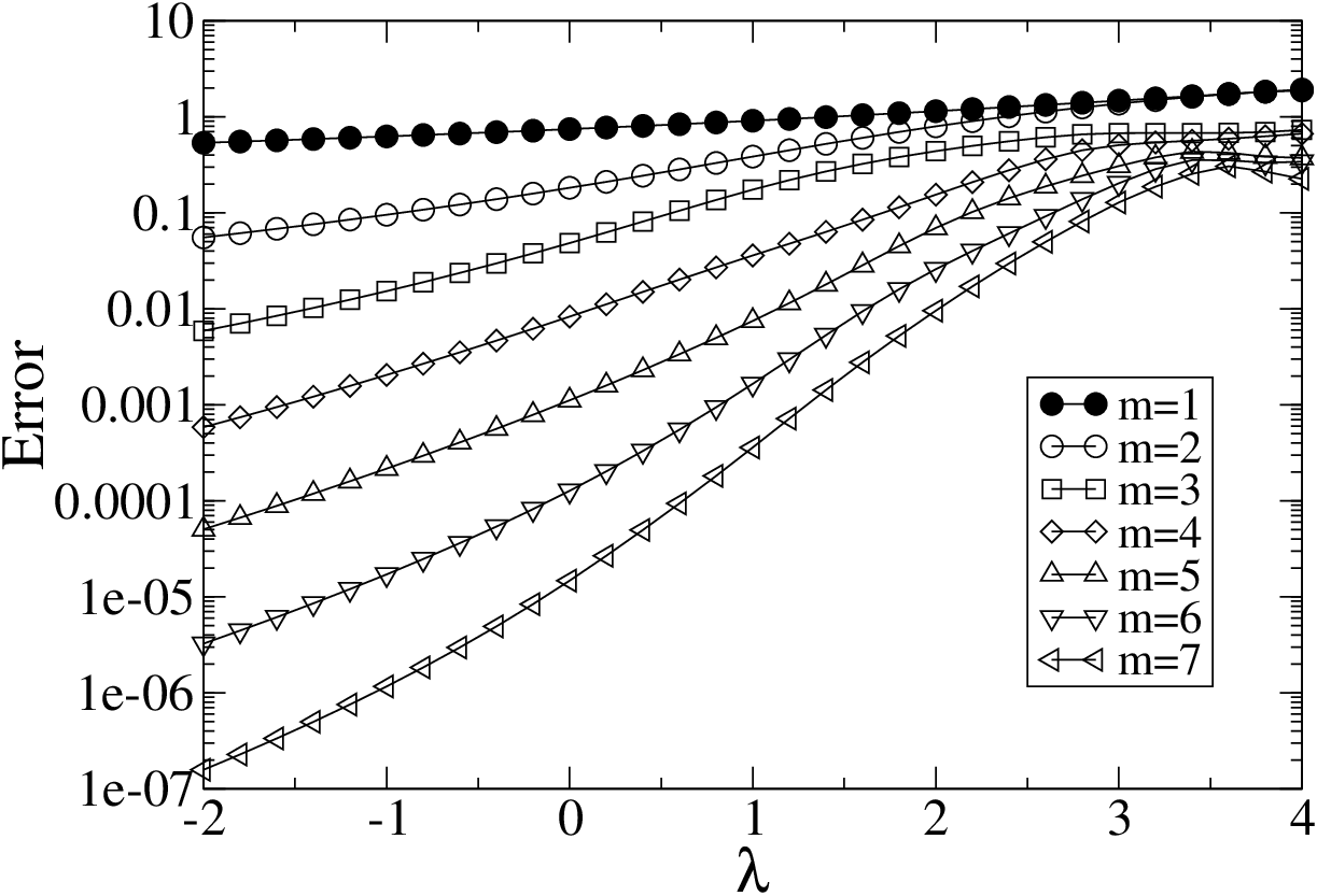

We next try the method on the more interesting case, though only the range needs to be tested as the matrix for can be mapped to with a diagonal scaling. The converged error norm for multiple values of and are plotted in Fig. 5. The condition number of the row normalized is less than twelve for all calculations performed. The decay of off the diagonal is exponential in geometric distance for , but this qualitative change in behavior from doesn’t cause any kinks in the error at . We observe that the exponential decay rate of error with is approximately proportional to . Near the point, the exponential error decay appears to break down leaving an error with an -dependence proportional to the logarithmic decay of off-diagonal elements of . The most obvious matrix property to attribute to the loss of decay near is the vanishing of the diagonal elements of .
The inverse proportionality between the condition number of the non-null subspace of Eq. (7) and the minimum error norm continues to hold as a function of as shown in Fig. 6. The condition number plotted is calculated at the converged value, but the condition number varies very little between iterations and it is within a factor of two of the condition number calculated from the initial guess.
The loss of exponential error decay as signifies the disappearance of locally removable degrees of freedom from a model restricted in form by the restriction on the sparsity pattern. As the wavelength of oscillations in the Helmholtz equation approaches four times the grid spacing, a high frequency limit where multigrid also fails. For the multigrid approach to continue into this limit, the solution must be decomposed into a sum of envelope functions times oscillatory solutions with wavevectors in various directions [9]. This is a transformation from a scalar differential equation to a vector differential equation, which can’t be represented by unless the sparsity pattern of is allowed to fill in somewhat. Error decay is restored for only because the discretization of the Helmholtz equation breaks down and the correct high frequency oscillations are no longer present in the matrix problem.
4 Choice of Sparsity Pattern
For all the tests performed in Section 3 we strictly prevented fill-in in transforming from to , but it is only really necessary to control fill-in enough to preserve the scalability of the factorization. It can be beneficial to add nonzero matrix elements to because that increases the number of degrees of freedom in the error minimization, Eq. (4), and can reduce the minimum error norm.
An important reason for filling in is to prevent the removal of a node from breaking the global connectivity of a problem. The simplest case of this is a tridiagonal matrix, which can be associated with a problem on a 1D grid. If a node is removed from the grid without filling in the matrix, then the grid will be split in half. The associated transformation would have to contain all the response of each half of the grid on the other and cannot in general be accurately made local.
One simple way to avoid changing the connectivity of a problem is to aggregate nodes together into supernodes where all the member nodes share all the connections of other member nodes. Once a supernode is formed, the decoupling of a node in the supernode won’t break any connectivity as long as one node remains within the supernode. The supernode concept has been used before in sparse Gaussian elimination for efficiency reasons [13] to allow for the use of dense matrix operations in inner loops, but here it serves a more fundamental purpose. The larger the supernodes are made, the more filled in the matrix will be, and the error norm will have a decreasing minimum with fixed local region size. If the supernodes are made large enough, then Gaussian elimination steps can be performed without additional matrix filling before the more expensive algebraic coarsening procedure in a possibly more efficient hybrid approach. For our example on a 2D grid, the grid of nodes can be made a grid of supernodes, which can be interpreted as a discretization of a vector differential equation where the number of vector components is the size of the supernode.
We again return to the test problem, now with a 2D grid of supernodes constructed by merging rectangles of neighboring nodes. A local transformation is performed to remove one node from one supernode and the local region is chosen to include all supernodes within hops of the removed node. The converged error norm for , is plotted in Fig. 7 and the important difference with Fig. 5 is the error seems to continue to decay exponentially in near rather than stagnate at . A comparison between three different supernode sizes is plotted in Fig. 8. For similar all errors are roughly the same in the non-oscillatory regime, , and at the maximally oscillatory point, , while the larger supernodes’ errors are smaller in the intermediate oscillatory regime, . This result suggests that supernodes are useful for increasing the rate of error decay, but if the case can indeed be improved, larger supernodes are required.


The arguments made in Ref. [9] suggest that at least an eight wave expansion is required for an efficient solution of the case, which might be properly captured by or . However, both cost and conditioning are a barrier to the current approach to calculating these transformations. The cost of solving the normal equation version of Eq. (7) for fixed local region size scales as . The conditioning of Eq. (7) remains inversely proportional to the minimum error norm, but the constant of proportionality is observed to change substantially with and , causing calculations to be more ill-conditioned with the same minimum error norms.
5 Conclusions
We have studied the possibility of factoring sparse matrices by means of local sparsity-preserving transformations with numerical tests of a single transformation. Intermediate stages of such a factorization require transformations to be performed on matrices of similar sparsity but with different values of their matrix elements, which was examined here in a simple, artificial manner by varying the frequency of the Helmholtz equation. Qualitatively, we expect the intermediate, “coarsened” matrices to still represent the Helmholtz equation with the frequency scaled to represent a change of length scale. The absence of local degrees of freedom for the case in Section 3.1 suggests that this interpretation fails when the wavelength becomes proportional to the grid spacing. To continue to remove local degrees of freedom beyond this frequency, it becomes necessary to allow the coarsened matrices to take a more general form.
The sparse linear solver methodology presented in this paper has demonstrated a behavior distinct from both direct and iterative solvers. The success of direct solvers is dependent on the filling in of the matrix in the intermediate stages of factorization, which is a graph theoretic property and is controlled by the order in which nodes are factored. The success of iterative solvers is dependent on the condition number of the matrix and is controlled by preconditioning a problem to reduce the condition number. Here the determining characteristic of how costly it is to solve a matrix is the decay of error of a transformation with respect to local region size and can be controlled by changing the local region or sparsity pattern. Matrix fill is no longer a problem as it is strictly controlled, and the error decay is a local property completely independent of the global spectrum and conditioning of the matrix.
There remain technical difficulties with calculating local sparsity-preserving transformations that must be resolved before a practical linear solver can be implemented with them. The most important problem is determining whether or not a well-conditioned process exists for calculating local transformations. The ill-conditioning is associated with minimizing an error norm, and a method based on additional criteria might precondition the process. Another important problem is understanding what properties of a matrix and sparsity pattern determine the rate of decay of error. This is needed to determine precisely when sparsity patterns should be changed and how they should be changed to make calculations most efficient. Once the issues associated with single transformations are resolved, there is the additional problem of choosing the ordering of transformations. The ordering can determine error decay rates of successive transformations, error propagation during factorization, and the amount to which the process can be parallelized. The simple answer at least for the purpose of parallelization is to choose as many transformations as possible on disjoint local regions to maximize the number of concurrent calculations of local transformations.
Acknowledgements
This work was supported by National Science Foundation Grant No. DMR04-39768 and by the Director, Office of Science, Office of Basic Energy Sciences, Division of Materials Sciences and Engineering, U.S. Department of Energy under Contract No. DE-AC03-76SF00098.
I would like to thank Professor Marvin Cohen for guidance and support.
I also thank Jay Deep Sau, David Bindel, Oren Livne, and Raim Tavisseur for numerous useful discussions.
References
- [1] G. H. Golub and C. F. Van Loan, Matrix Computations, 3rd ed. (John Hopkins University Press, Baltimore, 1996).
- [2] R. Barrett, M. Berry, T. F. Chan, J. Demmel, J. Donato, J. Dongarra, V. Eijkhout, R. Pozo, C. Romine, and H. Van der Vorst, Templates for the Solution of Linear Systems: Building Blocks for Iterative Methods, 2nd ed. (SIAM, Philadelphia, PA, 1994).
- [3] W. L. Briggs, V. E. Henson, and S. F. McCormick, A Multigrid Tutorial, 2nd ed. (SIAM, Philadelphia, PA, 2000).
- [4] W. Dahmen and A. Kunoth, Multilevel preconditioning, Numer. Math. 63, 315 (1992).
- [5] R. D. Falgout and P. S. Vassilevski, On generalizing the AMG framework, SIAM J. Numer. Anal. 42, 1669 (2004).
- [6] A. Brandt, General highly accurate algebraic coarsening, Electron. Trans. Numer. Anal. 10, 1 (2000).
- [7] J. W. Cooley and O. W. Tukey, An algorithm for the machine calculation of complex fourier series, Math. Comput. 19, 297 (1965).
- [8] R. Coifman, V. Rokhlin, and S. Wandzura, The fast multipole method for the wave equation: a pedestrian prescription, IEEE Antennas Propag. 35, 7 (1993).
- [9] A. Brandt and I. Livshits, Wave-ray multigrid method for standing wave equations, Electron. Trans. Numer. Anal. 6, 162 (1997).
- [10] A. George, Nested dissection of a regular finite element mesh, SIAM J. Numer. Anal. 10, 345 (1973).
- [11] H. C. Elman, O. G. Ernst, and D. P. O’Leary, A multigrid method enhanced by Krylov supspace iteration for discrete Helmholtz equations, SIAM J. Sci. Comput. 23, 1291 (2001).
- [12] M. Bebendorf and W. Hackbusch, Existence of -matrix approximants to the inverse FE-matrix of elliptic operators with -coefficients, Numer. Math. 95, 1 (2003).
- [13] J. W. Demmel, S. C. Eisenstat, J. R. Gilbert, X. S. Li, and J. W. H. Liu, A supernodal approach to sparse partial pivoting, SIAM J. Matrix Anal. A. 20, 720 (1999).