T-homotopy and refinement of observation (I) : Introduction

The main feature of the two algebraic topological models of higher dimensional automata (or HDA) introduced in [GG03] and in [Gau03] is to provide a framework for modelling continuous deformations of HDA corresponding to subdivision or refinement of observation. Globular complexes and flows are specially designed to model the weak S-homotopy equivalences (the spatial deformations) and the T-homotopy equivalences (the temporal deformations). The first descriptions of spatial deformation and of temporal deformation dates back from the informal and conjectural paper [Gau00].

Let us now explain a little bit what the spatial and temporal deformations consist of before presenting the results. The computer-scientific and geometric explanations of [GG03] must of course be preferred for a deeper understanding.

In dihomotopy theory, processes running concurrently cannot be distinguished by any observation. For instance in Figure 1, each axis of coordinates represents one process and the two processes are running concurrently. The corresponding geometric shape is a full $2$-cube. This example corresponds to the flow $\overrightarrow{C}_{2}$ defined as follows:

• •

  Let us introduce the flow $\partial\overrightarrow{C}_{2}$ defined by $(\partial\overrightarrow{C}_{2})^{0}=\{0,1,2,3\}$, $\mathbb{P}_{0,1}\partial\overrightarrow{C}_{2}=\{U\}$, $\mathbb{P}_{1,2}\partial\overrightarrow{C}_{2}=\{V\}$, $\mathbb{P}_{0,3}\partial\overrightarrow{C}_{2}=\{W\}$, $\mathbb{P}_{3,2}\partial\overrightarrow{C}_{2}=\{X\}$. The flow $\partial\overrightarrow{C}_{2}$ corresponds to an empty square, where the execution paths $U*V$ and $W*X$ are not running concurrently.

• •

  Then consider the pushout diagram

  with $q(\mathbf{S}^{0})=\{U*V,W*X\}$ (the globe functor ${\rm{Glob}}(-)$ is defined below). The presence of ${\rm{Glob}}(\mathbf{D}^{1})$ creates a S-homotopy between the execution paths $U*V$ and $W*X$, modelling this way the concurrency.

It does not matter for $\mathbb{P}_{0,2}\overrightarrow{C}_{2}$ to be homeomorphic to $\mathbf{D}^{1}$ or only homotopy equivalent to $\mathbf{D}^{1}$, or even only weakly homotopy equivalent to $\mathbf{D}^{1}$. The only fact that matters is that the topological space $\mathbb{P}_{0,2}\overrightarrow{C}_{2}$ be weakly contractible. Indeed, a hole like in the flow $\partial\overrightarrow{C}_{2}$ (the space $\mathbb{P}_{0,2}\partial\overrightarrow{C}_{2}$ is the discrete space $\{U*V,W*X\}$ ) means that the execution paths $U*V$ and $W*X$ are not running concurrently, and therefore that they are distinguishable by observation. This kind of identification is well taken into account by the notion of weak S-homotopy equivalence. This notion is introduced in [GG03] in the framework of globular complexes, in [Gau03] in the framework of flows and it is proved that these two notions are equivalent in [Gau05a].

In dihomotopy theory, it is also required to obtain descriptions of HDA which are invariant by refinement of observation. The simplest example of refinement of observation is represented in Figure 2, in which the directed segment $U$ is divided in two directed segments $U^{\prime}$ and $U^{\prime\prime}$. This kind of identification is well taken into account by the notion of T-homotopy equivalence. This notion is introduced in [GG03] in the framework of globular complexes, and in [Gau05a] in the framework of flows. The latter paper also proves that the two notions are equivalent. In the case of Figure 2, the T-homotopy equivalence is the unique morphism of flows sending $U$ to $U^{\prime}*U^{\prime\prime}$.

Each weak S-homotopy equivalence as well as each T-homotopy equivalence preserves as above the initial states and the final states of a flow. More generally, any good notion of dihomotopy equivalence must preserve the branching and merging homology theories introduced in [Gau05c]. This paradigm dates from the beginning of dihomotopy theory: a dihomotopy equivalence must not change the topological configuration of branching and merging areas of execution paths [Gou03]. It is also clear that any good notion of dihomotopy equivalence must preserve the underlying homotopy type, that is the topological space, defined only up to weak homotopy equivalence, obtained after removing the time flow. In the case of Figure 1 and Figure 2, this underlying homotopy type is the one of the point.

The initial object (resp. the terminal object) of a category $\mathcal{C}$, if it exists, is denoted by $\varnothing$ (resp. $\mathbf{1}$).

Let $\mathcal{C}$ be a cocomplete category. If $I$ is a set of morphisms of $\mathcal{C}$, then the class of morphisms of $\mathcal{C}$ that satisfy the RLP (right lifting property) with respect to any morphism of $I$ is denoted by $\inj(I)$ and the class of morphisms of $\mathcal{C}$ that are transfinite compositions of pushouts of elements of $I$ is denoted by $\cell(I)$. Denote by $\cof(I)$ the class of morphisms of $\mathcal{C}$ that satisfy the LLP (left lifting property) with respect to any morphism of $\inj(I)$. It is a purely categorical fact that $\cell(I)\subset\cof(I)$. Moreover, every morphism of $\cof(K)$ is a retract of a morphism of $\cell(K)$ as soon as the domains of $K$ are small relative to $\cell(K)$ ([Hov99] Corollary 2.1.15). An element of $\cell(I)$ is called a relative $I$-cell complex. If $X$ is an object of $\mathcal{C}$, and if the canonical morphism $\varnothing\longrightarrow X$ is a relative $I$-cell complex, one says that $X$ is a $I$-cell complex.

Let $\mathcal{C}$ be a cocomplete category with a distinguished set of morphisms $I$. Then let $\cell(\mathcal{C},I)$ be the full subcategory of $\mathcal{C}$ consisting of the objects $X$ of $\mathcal{C}$ such that the canonical morphism $\varnothing\longrightarrow X$ is an object of $\cell(I)$. In other terms, $\cell(\mathcal{C},I)=(\varnothing\!\downarrow\!\mathcal{C})\cap\cell(I)$.

Possible references for model categories are [Hov99], [Hir03] and [DS95]. The original reference is [Qui67] but Quillen’s axiomatization is not used in this paper. The axiomatization from Hovey’s book is preferred. If $\mathcal{M}$ is a cofibrantly generated model category with set of generating cofibrations $I$, let $\cell(\mathcal{M}):=\cell(\mathcal{M},I)$. A cofibrantly generated model structure $\mathcal{M}$ comes with a cofibrant replacement functor $Q:\mathcal{M}\longrightarrow\cell(\mathcal{M})$.

A partially ordered set $(P,\leqslant)$ (or poset) is a set equipped with a reflexive antisymmetric and transitive binary relation $\leqslant$. A poset is locally finite if for any $(x,y)\in P\times P$, the set $[x,y]=\{z\in P,x\leqslant z\leqslant y\}$ is finite. A poset $(P,\leqslant)$ is bounded if there exist $\widehat{0}\in P$ and $\widehat{1}\in P$ such that $P\subset[\widehat{0},\widehat{1}]$ and such that $\widehat{0}\neq\widehat{1}$. Let $\widehat{0}=\min P$ (the bottom element) and $\widehat{1}=\max P$ (the top element).

The category ${\rm{\mathbf{Top}}}$ of compactly generated topological spaces (i.e. of weak Hausdorff $k$-spaces) is complete, cocomplete and cartesian closed (more details for this kind of topological spaces in [Bro88, May99], the appendix of [Lew78] and also the preliminaries of [Gau03]). For the sequel, any topological space will be supposed to be compactly generated. A compact space is always Hausdorff.

The time flow of a higher dimensional automaton is encoded in an object called a flow [Gau03]. A flow $X$ consists of a set $X^{0}$ called the $0$-skeleton and whose elements correspond to the states (or constant execution paths) of the higher dimensional automaton. For each pair of states $(\alpha,\beta)\in X^{0}\times X^{0}$, there is a topological space $\mathbb{P}_{\alpha,\beta}X$ whose elements correspond to the (nonconstant) execution paths of the higher dimensional automaton beginning at $\alpha$ and ending at $\beta$. If $x\in\mathbb{P}_{\alpha,\beta}X$ , let $\alpha=s(x)$ and $\beta=t(x)$. For each triple $(\alpha,\beta,\gamma)\in X^{0}\times X^{0}\times X^{0}$, there exists a continuous map $*:\mathbb{P}_{\alpha,\beta}X\times\mathbb{P}_{\beta,\gamma}X\longrightarrow\mathbb{P}_{\alpha,\gamma}X$ called the composition law which is supposed to be associative in an obvious sense. The topological space $\mathbb{P}X=\bigsqcup_{(\alpha,\beta)\in X^{0}\times X^{0}}\mathbb{P}_{\alpha,\beta}X$ is called the path space of $X$. The category of flows is denoted by ${\rm{\mathbf{Flow}}}$. A point $\alpha$ of $X^{0}$ such that there are no non-constant execution paths ending to $\alpha$ (resp. starting from $\alpha$) is called an initial state (resp. a final state). A morphism of flows $f$ from $X$ to $Y$ consists of a set map $f^{0}:X^{0}\longrightarrow Y^{0}$ and a continuous map $\mathbb{P}f:\mathbb{P}X\longrightarrow\mathbb{P}Y$ preserving the structure. A flow is therefore “almost” a small category enriched in ${\rm{\mathbf{Top}}}$.

The category ${\rm{\mathbf{Flow}}}$ is equipped with the unique model structure such that [Gau03]:

• •

  The weak equivalences are the weak S-homotopy equivalences, i.e. the morphisms of flows $f:X\longrightarrow Y$ such that $f^{0}:X^{0}\longrightarrow Y^{0}$ is a bijection and such that $\mathbb{P}f:\mathbb{P}X\longrightarrow\mathbb{P}Y$ is a weak homotopy equivalence.

• •

  The fibrations are the morphisms of flows $f:X\longrightarrow Y$ such that $\mathbb{P}f:\mathbb{P}X\longrightarrow\mathbb{P}Y$ is a Serre fibration.

This model structure is cofibrantly generated. The set of generating cofibrations is the set $I^{gl}_{+}=I^{gl}\cup\{R,C\}$ with

where $\mathbf{D}^{n}$ is the $n$-dimensional disk, where $\mathbf{S}^{n-1}$ is the $(n-1)$-dimensional sphere, where $R$ and $C$ are the set maps $R:\{0,1\}\longrightarrow\{0\}$ and $C:\varnothing\longrightarrow\{0\}$ and where for any topological space $Z$, the flow ${\rm{Glob}}(Z)$ is the flow defined by ${\rm{Glob}}(Z)^{0}=\{\widehat{0},\widehat{1}\}$, $\mathbb{P}{\rm{Glob}}(Z)=Z$, $s=\widehat{0}$ and $t=\widehat{1}$, and a trivial composition law. The set of generating trivial cofibrations is

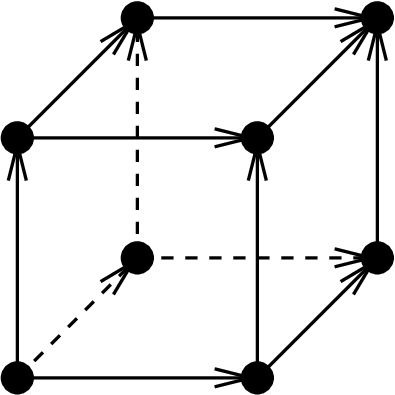
It turns out that the T-homotopy equivalences, as defined in [Gau05a], are the deformations which locally act like in Figure 2 ¹¹ 1 This fact was of course not known when [GG03] was being written down. The definition of T-homotopy equivalence presented in that paper was based on the notion of homeomorphism and it sounded so natural…. So it becomes impossible with this old definition to identify the directed segment of Figure 2 with the full $3$-cube of Figure 4 by a zig-zag sequence of weak S-homotopy and of T-homotopy equivalences preserving the initial state and the final state of the $3$-cube since any point of the $3$-cube is related to three distinct edges (cf. Theorem 3.4). This contradicts the fact that concurrent execution paths cannot be distinguished by observation. More precisely, one has:

Notice that for $n\geqslant 2$, the flow $\overrightarrow{I}^{\otimes n}$ is not cofibrant. Indeed, the composition law contains relations. For instance, with $n=2$, one has $(\widehat{0},u)*(u,\widehat{1})=(u,\widehat{0})*(\widehat{1},u)$

In the statement of Theorem 3.4, we suppose that each flow $X_{i}$ belongs to ${\cell({\rm{\mathbf{Flow}}})}$ because T-homotopy is only defined between this kind of flow.

We need to generalize the notion of subdivision of the directed segment $\overrightarrow{I}$.

A flow $X$ is loopless if and only if the transitive closure of the set $\{(\alpha,\beta)\in X^{0}\times X^{0}\hbox{ such that }\mathbb{P}_{\alpha,\beta}X\neq\varnothing\}$ induces a partial ordering on $X^{0}$.

Let $\overrightarrow{D}$ be a full directed ball. Then the set $\overrightarrow{D}^{0}$ can be viewed as a finite bounded poset. Conversely, if $P$ is a finite bounded poset, let us consider the flow $F(P)$ associated to $P$: it is of course defined as the unique flow (up to isomorphism) $F(P)$ such that $F(P)^{0}=P$ and $\mathbb{P}_{\alpha,\beta}F(P)=\{u\}$ if $\alpha<\beta$ and $\mathbb{P}_{\alpha,\beta}F(P)=\varnothing$ otherwise. Then $F(P)$ is a full directed ball and for any full directed ball $\overrightarrow{D}$, the two flows $\overrightarrow{D}$ and $F(\overrightarrow{D}^{0})$ are weakly S-homotopy equivalent.

Let $\overrightarrow{E}$ be another full directed ball. Let $f:\overrightarrow{D}\longrightarrow\overrightarrow{E}$ be a morphism of flows preserving the initial and final states. Then $f$ induces a morphism of posets from $\overrightarrow{D}^{0}$ to $\overrightarrow{E}^{0}$ such that $f(\min\overrightarrow{D}^{0})=\min\overrightarrow{E}^{0}$ and $f(\max\overrightarrow{D}^{0})=\max\overrightarrow{E}^{0}$. Hence the following definition:

A T-homotopy consists of locally replacing in a flow a full directed ball by a more refined one (cf. Figure 5).

In a HDA, a $n$-transition, that is the concurrent execution of $n$ processes, is represented by the full $n$-cube $\overrightarrow{C}_{n}$. The corresponding poset is the product poset $\{\widehat{0}<\widehat{1}\}^{n}$. In particular, the poset corresponding to the full directed ball of Figure 4 is $\{\widehat{0}<\widehat{1}\}^{3}=\{\widehat{0}<\widehat{1}\}\times\{\widehat{0}<\widehat{1}\}\times\{\widehat{0}<\widehat{1}\}$.

The poset corresponding to Figure 1 is the poset $\{\widehat{0}<\widehat{1}\}^{2}=\{\widehat{0}<\widehat{1}\}\times\{\widehat{0}<\widehat{1}\}$. If for instance $U$ is subdivided in two processes as in Figure 2, the poset of the full directed ball of Figure 1 becomes equal to $\{\widehat{0}<2<\widehat{1}\}\times\{\widehat{0}<\widehat{1}\}$.

One has the isomorphism of flows $\overrightarrow{I}^{\otimes n}\cong F(\{\widehat{0}<\widehat{1}\}^{n})$ for every $n\geqslant 1$. The flow $\overrightarrow{C}_{n}$ ($n\geqslant 1$) is identified to $\overrightarrow{I}$ by the zig-zag sequence of S-homotopy and generalized T-homotopy equivalences

where $g_{n}:\{\widehat{0}<\widehat{1}\}\longrightarrow\{\widehat{0}<\widehat{1}\}^{n}\in\mathcal{T}$.

First of all, we must verify that each old T-homotopy equivalence as defined in [Gau05a] will be a particular case of this new definition. And indeed, one has:

The two other tests consist of verifying that the branching and merging homology theories [Gau05c], as well as the underlying homotopy type functor [Gau05a] are preserved with this new definition of T-homotopy equivalence. And indeed, one has:

This new definition of T-homotopy equivalence seems to be well-behaved. It will hopefully have a longer lifetime than other ones that the author proposed in the past. It is already known after [Gau05b] that it is impossible to construct a model structure on ${\rm{\mathbf{Flow}}}$ such that the weak equivalences are exactly the weak S-homotopy equivalences and the generalized T-homotopy equivalences. So new models of dihomotopy will be probably necessary to understand the T-homotopy equivalences.

References

- [Bro88] R. Brown. Topology. Ellis Horwood Ltd., Chichester, second edition, 1988. A geometric account of general topology, homotopy types and the fundamental groupoid.
- [DS95] W. G. Dwyer and J. Spaliński. Homotopy theories and model categories. In Handbook of algebraic topology, pages 73–126. North-Holland, Amsterdam, 1995.
- [Gau00] P. Gaucher. From concurrency to algebraic topology. In Electronic Notes in Theoretical Computer Science, volume 39, page 19pp, 2000.
- [Gau03] P. Gaucher. A model category for the homotopy theory of concurrency. Homology, Homotopy and Applications, 5(1):p.549–599, 2003.
- [Gau05a] P. Gaucher. Comparing globular complex and flow. New York Journal of Mathematics, 11:p.97–150, 2005.
- [Gau05b] P. Gaucher. Flow does not model flows up to weak dihomotopy. Applied Categorical Structures, 13:371–388, 2005.
- [Gau05c] P. Gaucher. Homological properties of non-deterministic branchings and mergings in higher dimensional automata. Homology, Homotopy and Applications, 7(1):p.51–76, 2005.
- [GG03] P. Gaucher and E. Goubault. Topological deformation of higher dimensional automata. Homology, Homotopy and Applications, 5(2):p.39–82, 2003.
- [Gou03] E. Goubault. Some geometric perspectives in concurrency theory. Homology, Homotopy and Applications, 5(2):p.95–136, 2003.
- [Hir03] P. S. Hirschhorn. Model categories and their localizations, volume 99 of Mathematical Surveys and Monographs. American Mathematical Society, Providence, RI, 2003.
- [Hov99] M. Hovey. Model categories. American Mathematical Society, Providence, RI, 1999.
- [Lew78] L. G. Lewis. The stable category and generalized Thom spectra. PhD thesis, University of Chicago, 1978.
- [May99] J. P. May. A concise course in algebraic topology. University of Chicago Press, Chicago, IL, 1999.
- [Qui67] D. G. Quillen. Homotopical algebra. Springer-Verlag, Berlin, 1967.