跳到论文正文
W Papers独立论文阅读器 arXiv:math/0505121 论文正文 计算阅读时间 · 0%
引用这篇论文根据当前论文元数据生成,正式投稿前建议核对。


License: Assumed arXiv.org perpetual non-exclusive license
arXiv:math/0505121v1 [math.DG] 07 May 2005

Residue Formulation of Chern Character on Smooth ManifoldsThanks:  The author expresses his most sincere gratitude to his thesis advisor, professor Nigel Higson for invaluable guidance, patience and summer support.

Dmitry Gerenrot Address:  Dmitry Gerenrot, Georgia Institute of Technology, School of Mathematics, 686 Cherry Street, Atlanta, GA, 30332-0160, U.S.A. Email address: gerenrot@math.gatech.edu
Date: August 11, 2026
Abstract.

The Chern character of a complex vector bundle is most conveniently defined as the exponential of a curvature of a connection. It is well known that its cohomology class does not depend on the particular connection chosen. It has been shown by Quillen [12] that a connection may be perturbed by an endomorphism of the vector bundle, such as a symbol of some elliptic differential operator. This point of view, as we intend to show, allows one to relate Chern character to a non-commutative sibling formulated by Connes and Moscovici [7]. The general setup for our problem is purely geometric. Let σ\sigma be the symbol of a Dirac-type operator acting on sections of a ℤ2{{\mathbb{Z}}}_{2}-graded vector bundle EE. Let ∇\nabla be a connection on EE, pulled back to T∗​MT^{*}M. Suppose also that ∇\nabla respects the ℤ2{{\mathbb{Z}}}_{2}-grading. The object ∇+σ\nabla+\sigma is a superconnection on T∗​MT^{*}M in the sense of Quillen. We obtain a formula for the H∗​(M)H_{*}(M)-valued Poincare dual of Quillen’s Chern character c​h​(D)=trs⁡e(∇+σ)2ch(D)=\operatorname{tr_{s}}e^{(\nabla+\sigma)^{2}} in terms of residues of Γ⁡(z)​trs⁡(∇+σ)−2​z\Gamma(z)\operatorname{tr_{s}}(\nabla+\sigma)^{-2z}. We also compute two examples.

Key words and phrases: 
Noncommutative Geometry Chern Character Connes Moscovici Quillen Superconnection Residue Cocycle

1. Introduction.

The historical background for noncommutative index theory has two basic parts. The first one dates back to the nineteen fifties, when Israel Gelfand pointed out to Sir Michael Atiyah that the index of a Fredholm operator was stable under small perturbations. The ultimate consequence of this remark is quite famous: the Atiyah-Singer Index Theorem [2, 3, 4]. The second part is development of noncommutative geometry by Alain Connes [6, 8].

In particular, two noncommutative versions of the Chern character were developed. There is one due to Connes [5] and a more recent one due to Connes and Moscovici [7]. We are interested in this more recent version, which is called the residue cocycle. Its individual terms are certain residues which are geometrically interesting, as pointed out by Higson. However, they are not very well understood.

In the present paper, we shall prove a formula which resembles the formula of Connes and Moscovici in [7], albeit in a classical setting. Suppose MM is a compact smooth manifold with no boundary. Let E→ME\rightarrow M be a ℤ2{{\mathbb{Z}}}_{2}-graded complex vector bundle. Let DD be an elliptic, odd, first-order, skew-adjoint differential operator on EE. Finally, let π:T∗​M→M\pi\colon\thinspace T^{*}M\to M be the standard projection map of the cotangent bundle. With this setup, we will establish a formula for the Chern character of the symbol of DD which resembles the Connes-Moscovici Chern character in noncommutative geometry. It is comprised of finitely many residues of zeta functions constructed from the symbol of DD and a connection on EE.

We shall use Quillen’s formalism in which the symbol LL of DD, together with a connection on EE, determines a superconnection on π∗​E\pi^{*}E [12]. Quillen’s superconnection ∇+L\nabla+L encodes all the information necessary to define the Chern character in a single object. We shall denote it by ∇L\nabla_{L}.

The supertrace of exp⁡∇L2\exp\nabla_{L}^{2} is a mixed differential form which enjoys the major properties of the ordinary Chern character: it is closed and its cohomology class depends only on the underlying vector bundle, not on ∇\nabla or LL. But rather than passing to its cohomology class on T∗​MT^{*}M, we take advantage of the fact that this form is rapidly decreasing on the fibers of T∗​MT^{*}M. We get this convenient property by sacrificing the traditional −12​π​i{\frac{-1}{2\pi i}} factor, an error which we shall also address. Thus, we define a current on Ω∗​M\Omega^{*}M by the Poincare Duality formula

P​D:η↦∫T∗​Mπ∗​(η)​trs⁡exp⁡∇L2.PD\colon\thinspace\eta\mapsto\int_{T^{*}M}\pi^{*}(\eta)\operatorname{tr_{s}}\exp\nabla_{L}^{2}.

If we expand this dual “Chern character current” in the Taylor series, we obtain:

P​D​[trs⁡exp⁡∇L2]=P​D​[trs⁡(1+∇L+12!​∇L2+…)]PD\left[\operatorname{tr_{s}}\exp\nabla_{L}^{2}\right]=PD\left[\operatorname{tr_{s}}(1+\nabla_{L}+{\frac{1}{2!}}\nabla_{L}^{2}+\ldots)\right]

The terms on the right are closed forms and their cohomology classes depend on the isomorphism type of π∗​E\pi^{*}E only. However, they are not rapidly decreasing and we cannot form the dual currents by coupling them with the pullback of an arbitrary smooth form on MM.

We resolve this issue through analytic regularization, to be addressed in section 3, and thus obtain a new formula for the dual Chern character. Briefly, our main result can be stated as follows:

Theorem. For R>0R>0, let YRY_{R} be the RR-tubular neighborhood of the zero section of T∗​MT^{*}M. Then:

∫T∗​Mπ∗​(η)\displaystyle\int_{T^{*}M}\pi^{*}(\eta) trs⁡exp⁡∇L2\displaystyle\operatorname{tr_{s}}\exp\nabla_{L}^{2}
=limR→0∑z∈ℂR​e​s|z​[Γ⁡(z)​∫T∗​M\YRπ∗​(η)​trs⁡(−∇L)−2​z].\displaystyle=\lim_{R\to 0}\sum_{z\in{{\mathbb{C}}}}Res|_{z}\Big[\Gamma(z)\int_{T^{*}M\backslash Y_{R}}\pi^{*}(\eta)\operatorname{tr_{s}}(-\nabla_{L})^{-2z}\Big].

The limit arises due to divergence of negative powers of LL near zero.

We now proceed to briefly describe the Connes-Moscovici local Chern character, i.e., the noncommutative Chern character.

The Chern character in [7] is a periodic cyclic cohomology class in H​P​C∗HPC^{*}. This cohomology is constructed from spaces of multilinear functionals on AA. See [8], chapter 10, for construction of H​P​C∗HPC^{*}. The Connes-Moscovici Chern character is represented by a sequence of multilinear functionals on AA which we proceed to describe. The n-th term of the sequence is zero for n=1,3,5,…n=1,3,5,\ldots; for n=0,2,4​…n=0,2,4\ldots, let a0,a1,…​ana_{0},a_{1},\ldots a_{n} be the elements of AA. Let Trs\operatorname{Tr_{s}} be the supertrace and let kk be the variable running through all nn-multiindices with nonnegative integer entries.

ϕ⁡(a0,a1,…​an)=\displaystyle\phi(a_{0},a_{1},\ldots a_{n})= ∑kCn​k​R​e​s|z=0​Γ​(z+|k|+n2)\displaystyle\sum_{k}C_{nk}Res|_{z=0}\Gamma(z+|k|+{\frac{n}{2}})
×Trs⁡(a0​δ(k1)​([D,a1])​…​δ(kn)​([D,an])​D−2​(z+|k|+n2)),\displaystyle\,\,{\scriptstyle\times}\operatorname{Tr_{s}}\left({\scriptstyle a_{0}}\delta^{(k_{1})}({\scriptstyle[D,a_{1}]})\ldots\delta^{(k_{n})}({\scriptstyle[D,a_{n}]})D^{-2(z\!+\!|k|\!+\!{\frac{n}{2}})}\right),

where

Cn​k=(−1)|k|​Γ​(n2+|k|)k!​(k1+1)​(k1+k2+2)​…​(k1+k2+…​kn+n).C_{nk}={\frac{(-1)^{|k|}\Gamma({\frac{n}{2}}+|k|)}{k!(k_{1}+1)(k_{1}+k_{2}+2)\ldots(k_{1}+k_{2}+\ldots k_{n}+n)}}.

Also, note that the trace T​rs​(…​D−2​(z+|k|+n2))Tr_{s}(\ldots\,D^{-2(z+|k|+{\frac{n}{2}})}) must be replaced by its meromorphic continuation in zz, before we take the residues. Existence of such a continuation is also implied by certain axioms and is not trivial at all. Indeed, as it stands, the operators whose trace we are taking typically fail to be bounded, let alone trace class.

To us, the most important fact about the Connes-Moscovici formula is that this Chern character is a sum of residues of T​rs​(…​D−2​(z+|k|+n2))Tr_{s}(\ldots\,D^{-2(z+|k|+{\frac{n}{2}})}) times the gamma function. Our main result expresses the Quillen’s representative of the (classical) Chern character as a sum of very similar quantities. Much like the proof in [7], our argument hinges on the Mellin transform.

2. Superconnections and Chern Classes.

In this section, we give an overview of superconnections according to Quillen [12]. This notion shall be used to define Chern character in the spirit of Chern-Weil theory. Let MM be a smooth manifold with no boundary. Let EE be a smooth complex ℤ2{{\mathbb{Z}}}_{2}-graded vector bundle over MM. We work with the vector bundle Λ∗​M⊗E.\Lambda^{*}M\otimes E.

Definition 2.1.

(Quillen, [12]) Let 𝐚⁡(E){{\mathbf{a}}}(E) be the space of smooth sections of the vector bundle Λ∗​M⊗E​n​d​(E).\Lambda^{*}M\otimes End(E). It naturally inherits the ℤ2{{\mathbb{Z}}}_{2}-grading from the fibers.

Definition 2.2.

Let ω,ν\omega,\,\nu be homogeneous differential forms on MM, let T,S∈Γ∞​E​n​d​(E)T,S\in\Gamma^{\infty}End(E) be homogeneous (purely even or purely odd) endomorphisms of EE and let s∈Γ∞​(Λ∗​M⊗E)s\in\Gamma^{\infty}(\Lambda^{*}M\otimes E) be a homogeneous section. We define the graded multiplication on 𝐚⁡(E){{\mathbf{a}}}(E) by:

(1) (ω⊗T)(ν⊗S)=d​e​f(−1)d​e​g​(ν)​d​e​g​(T)ων⊗TS(\omega\otimes T)\,(\nu\otimes S)=_{def}(-1)^{deg(\nu)deg(T)}\omega\nu\otimes TS

Also, the action of 𝐚⁡(E){{\mathbf{a}}}(E) on Γ∞​(Λ∗​M⊗E)\Gamma^{\infty}(\Lambda^{*}M\otimes E) is defined by:

(2) (ω⊗T)(ν⊗s)=d​e​f(−1)d​e​g​(ν)​d​e​g​(T)Tν⊗Ts(\omega\otimes T)\,(\nu\otimes s)=_{def}(-1)^{deg(\nu)deg(T)}T\nu\otimes Ts
Lemma 2.1.

The equation (1) makes 𝐚⁡(E){{\mathbf{a}}}(E) an associative superalgebra. Also, (2) defines an algebra action of 𝐚⁡(E){{\mathbf{a}}}(E) on Γ∞​(Λ∗​M⊗E).\Gamma^{\infty}(\Lambda^{*}M\otimes E). In fact, this makes 𝐚⁡(E){{\mathbf{a}}}(E) a subalgebra of Γ∞​E​n​d​(Λ∗​M⊗E)\Gamma^{\infty}End(\Lambda^{*}M\otimes E) in the sense that no nonzero element of 𝐚⁡(E){{\mathbf{a}}}(E) kills everything. ∎

The condition (2) is called Ω∗\Omega^{*}-linearity. It turns out that Ω∗\Omega^{*}-linear endomorphisms of Λ∗​M⊗E\Lambda^{*}M\otimes E are precisely the elements of 𝐚⁡(E){{\mathbf{a}}}(E).

Lemma 2.2.

The algebra 𝐚⁡(E){{\mathbf{a}}}(E) is the ℂ{{\mathbb{C}}}-span of homogeneous smooth sections of E​n​d±​((Λ∗​M)⊗E)End^{\pm}(\big(\Lambda^{*}M\big)\otimes E) which are in addition Ω∗\Omega^{*}-linear. ∎

Remark 2.1.

Observe that 𝐚⁡(E){{\mathbf{a}}}(E) is naturally a left Ω∗​M\Omega^{*}M-module.

Remark 2.2.

The definition 2.2 resembles the usual definition of multiplication on a tensor product of two algebras. However, it takes the ℤ2{{\mathbb{Z}}}_{2}-grading into account. Such products of superalgebras are called graded tensor products and are denoted by ⊗^\hat{\otimes}.

Next, observe that the ℤ2{{\mathbb{Z}}}_{2}-grading on EE naturally induces one on the space of sections Γ∞​(Λ∗​M⊗E)\Gamma^{\infty}(\Lambda^{*}M\otimes E), which makes it possible to speak of even and odd linear endomorphisms of this space. The even ones preserve the ℤ2{{\mathbb{Z}}}_{2} grading and the odd ones switch it. We are now ready to define superconnections.

Definition 2.3.

Let EE be a smooth ℤ2{{\mathbb{Z}}}_{2}-graded complex vector bundle. In the spirit of [12], we define a superconnection on EE to be an odd ℂ{{\mathbb{C}}}-linear map

∇:Γ∞​(Λ∗​M⊗E)→Γ∞​(Λ∗​M⊗E),\nabla\colon\thinspace\Gamma^{\infty}(\Lambda^{*}M\otimes E)\to\Gamma^{\infty}(\Lambda^{*}M\otimes E),

which satisfies the so-called graded Leibniz rule:

∇(ωs)=(dω)s+(−1)d​e​g​(ω)ω∇s.\nabla(\omega s)=(d\omega)s+(-1)^{deg(\omega)}\omega\nabla s.

The curvature of ∇\nabla is defined as ∇2.\nabla^{2}.

Lemma 2.3.

The curvature is a globally well-defined, even element of 𝐚⁡(E).{{\mathbf{a}}}(E).∎

Lemma 2.4.

Locally, any superconnection is always of the form
d⊗i​d+θd\otimes id+\theta, where dd is the de Rham differential and θ\theta is a local odd section of Λ∗​M⊗E​n​d​(E).\Lambda^{*}M\otimes End(E). ∎

Corollary 2.5.

Given a superconnection ∇\nabla and an arbitrary odd element LL of 𝐚⁡(E){{\mathbf{a}}}(E), ∇+L\nabla+L is also a superconnection.

Lemma 2.6.

Any connection which respects the ℤ2{{\mathbb{Z}}}_{2}-grading is a superconnection.

Proof: Such a connection can be locally written as d+θd+\theta, where θ=(d​xi​Γi​jk)j​k\theta=(dx_{i}\Gamma^{k}_{ij})_{jk} is a matrix of 1-forms. Since the connection respects the grading, the matrices (Γi​jk)i​k(\Gamma_{ij}^{k})_{ik} define even endomorphisms of EE. Presence of 1-forms, therefore, makes θ\theta odd.∎

Definition 2.4.

We denote the superconnection ∇+L\nabla+L by ∇L\nabla_{L}.

Definition 2.5.

Suppose WW is a finite-dimensional ℤ2{{\mathbb{Z}}}_{2}-graded complex vector space and A=E​n​d​(W)A=End(W). We define the supertrace trsℂ:A→ℂ\operatorname{tr_{s}}^{{\mathbb{C}}}\colon\thinspace A\to{{\mathbb{C}}} by the following equation:

∀f=(f11f12f21f22)∈A,trsℂ(f)=d​e​ftr(f11)−tr(f22),\forall f=\left(\begin{array}[]{cc}f_{11}&f_{12}\\ f_{21}&f_{22}\\ \end{array}\right)\in A,\,\,\operatorname{tr_{s}}^{{\mathbb{C}}}(f)=_{def}\operatorname{tr}(f_{11})-\operatorname{tr}(f_{22}),

where the traces on the right hand side are the usual traces of operators from W+W^{+} and W−W^{-} into themselves. Let RR be another ℤ2{{\mathbb{Z}}}_{2}-graded algebra. A typical simple tensor in R​⊗^​AR\hat{\otimes}A has the form

f=(r11​f11r12​f12r21​f21r22​f22).f=\left(\begin{array}[]{cc}r_{11}f_{11}&r_{12}f_{12}\\ r_{21}f_{21}&r_{22}f_{22}\\ \end{array}\right).

On simple tensors, we define trsR:R​⊗^​A→R\operatorname{tr_{s}}^{R}\colon\thinspace R\hat{\otimes}A\to{R} by

r11​t⁡r⁡(f11)−(−1)d​e​g​(r22)​r22​t⁡r⁡(f22).r_{11}{\operatorname{t}r}(f_{11})-(-1)^{deg(r_{22})}r_{22}{\operatorname{t}r}(f_{22}).

If WW is a fiber of some vector bundle EE, this definition extends naturally to sections.

We proceed toward the definition of Chern character. To that end, we need the graded version of the trace. Being ℤ2{{\mathbb{Z}}}_{2}-graded, E​n​d​(E)End(E) has a supertrace trsℂ:E​n​d​(E)→ℂ\operatorname{tr}^{{\mathbb{C}}}_{s}\colon\thinspace End(E)\to{{\mathbb{C}}} which means that on Λ∗​M​⊗^​E​n​d​(E)\Lambda^{*}M\hat{\otimes}End(E) the Λ∗​V\Lambda^{*}V-valued supertrace trΛ∗​M:Λ∗​M⊗(E)→Λ∗​M\operatorname{tr}^{\Lambda^{*}M}\colon\thinspace\Lambda^{*}M\otimes(E)\to\Lambda^{*}M makes sense.

Definition 2.6.

The 2​k2k-th component of the Chern character form is defined as the following differential form:

c​h2​k​(E)=1k!​trsΛ∗​M⁡(∇2​k)∈Ω2​k​M.ch_{2k}(E)={\frac{1}{k!}}\operatorname{tr_{s}}^{\Lambda^{*}M}(\nabla^{2k})\in\Omega^{2k}M.

The total Chern character form is

c​h​(E)=∑k=0∞c​hk​(E).ch(E)=\sum_{k=0}^{\infty}ch_{k}(E).

We usually write this form as trsΛ∗​M⁡(exp⁡(∇2))\operatorname{tr_{s}}^{\Lambda^{*}M}(\exp(\nabla^{2})).

Theorem 2.7.

(Quillen, [12]). The series defining c​h​(E)ch(E) converges.∎

Theorem 2.8.

([12]) c​hkch_{k} is closed and its cohomology class is independent on a choice of the superconnection. This class is an invariant of isomorphism classes of complex vector bundles.∎

3. Formulation of the Problem.

Here we state the main theorems of the paper. The proofs shall be given in subsequent sections.

The general geometric setup for our problem is the following. Let MM be a compact, nn-dimensional, smooth manifold. Let E→ME\rightarrow M be a smooth, ℤ2{{\mathbb{Z}}}_{2}-graded complex vector bundle. We assume that EE and T​MTM are provided with metrics. Let DD be an elliptic, odd, first-order, selfadjoint differential operator on EE. Finally, let π:T∗​M→M\pi\colon\thinspace T^{*}M\to M be the standard projection map of the cotangent bundle, and let ∇\nabla be a superconnection on π∗​E\pi^{*}E which arises as a pullback of some superconnection ∇′\nabla^{\prime} from EE.

Our result is motivated by the Connes-Moscovici formula. We express the right-hand side of the Atiyah-Singer Index Theorem in a way which resembles their residue cocycle. Namely, we shall sum over all the residues of the expression:

Γ⁡(z)​∫T∗​Mπ∗​(η)​∇L−2​z.\Gamma(z)\int_{T^{*}M}\pi^{*}(\eta)\nabla_{L}^{-2z}.

The Index Theorem using Quillen’s Chern charactrer can be stated as:

I​n​d​(D)=∑κ(−12​π​i)2​n−κ​∫T∗​Mπ∗​(T​o​𝑑d​[T​M⊗ℂ])κ​c​h​(L).Ind(D)=\sum_{\kappa}\big({\frac{-1}{2\pi i}}\big)^{2n-\kappa}\int_{T^{*}M}\pi^{*}(Todd[TM\otimes{{\mathbb{C}}}])_{\kappa}ch(L).

Here we need to prove that the integral (lemma 3.1) converges and that c​h​(L)ch(L) may indeed be used in place of the ordinary chern character (theorem 3.3). The factor of (−12​π​i)2​n−κ({\frac{-1}{2\pi i}})^{2n-\kappa} is to correct for the error introduced by leaving the 2​π​i2\pi i out of Quillen’s definition of Chern chracter.

The right-hand side is really concerned with the Poincare Dual of c​h​(L)ch(L), i.e. with the following linear functional

P​D​[c​h​(L)]:η↦∫T∗​Mπ∗​(η)​c​h​(L).PD[ch(L)]\colon\thinspace\eta\mapsto\int_{T^{*}M}\pi^{*}(\eta)ch(L).
Lemma 3.1.

The quantity ‖c​h​(L)‖=‖trs⁡exp⁡∇L2‖\|ch(L)\|=\|\operatorname{tr_{s}}\exp\nabla_{L}^{2}\| decays exponentially along the fibers of T∗​MT^{*}M. In fact, there are positive constants CC and KK such that

‖c​h​(L)‖≤C​e−K​ρ2,\|ch(L)\|\leq Ce^{-K\rho^{2}},

where ρ\rho is the radial coordinate on the fibers of T∗​MT^{*}M obtained from the Riemanian metric.

Corollary 3.2.

Since MM is compact, the integral ∫T∗​Mπ∗​(η)​c​h​(L)\int_{T^{*}M}\pi^{*}(\eta)ch(L) converges.

The necessary estimates for this lemma are provided in section 3 of [12]. Essentially, it is true because DD is selfadjoint, so that LL is antiselfadjoint and L2L^{2} is negative-definite, which is where the ellipticity of DD comes in. Also, L2L^{2} increases polynomially on the fibers of T∗​MT^{*}M. When we exponentiate ∇L2=∇2+[∇,L]+L2\nabla^{2}_{L}=\nabla^{2}+[\nabla,L]+L^{2}, the resulting expression decreases as e−K​r2e^{-Kr^{2}}.

Next consider the Taylor expansion of c​h​(L)ch(L):

trs⁡exp⁡∇L2=trs⁡(1+∇L+12!​∇L2+…).\operatorname{tr_{s}}\exp\nabla_{L}^{2}=\operatorname{tr_{s}}(1+\nabla_{L}+{\frac{1}{2!}}\nabla_{L}^{2}+\ldots).

Although the Poincare dual of the left-hand side converges, the duals the individual Taylor terms do not, due to polynomial increase of LL along the fibers of T∗​MT^{*}M.

We get around this difficulty by analytic regularization. The general idea is that if we replace the integer power kk of ∇L2\nabla^{2}_{L} by a complex number −z-z, where R​e​(z)≫1Re(z)\gg 1, we also can replace the integral 1k!​∫T∗​Mπ∗​(η)​∇L2​k{\frac{1}{k!}}\int_{T^{*}M}\pi^{*}(\eta)\nabla^{2k}_{L} with the following expression:

(3) R​e​s|z=−k​Γ​(z)​∫T∗​Mπ∗​(η)​∇L−2​z.Res|_{z=-k}\Gamma(z)\int_{T^{*}M}\pi^{*}(\eta)\nabla^{-2z}_{L}.

Before we can take this residue, though, we need to pass to the meromorphic extension of

(4) ∫T∗​Mπ∗​(η)​∇L−2​z.\int_{T^{*}M}\pi^{*}(\eta)\nabla^{-2z}_{L}.

In particular, we need to prove that such an extension exists (theorem 3.4).

However, there is yet another difficulty. Let |⁣||\,\,| denote the fiberwise norm on T∗​MT^{*}M. Define:

YR=d​e​f{ξ∈T∗M:|ξ|<R}.Y_{R}=_{def}\{\xi\in T^{*}M\colon\thinspace|\xi|<R\}.
XR=d​e​fYRc.X_{R}=_{def}Y_{R}^{c}.

The integral in (4) would not really converge, if taken over all of T∗​MT^{*}M, because L2L^{2} is a symbol of a second-order differential operator. Hence, L2L^{2} is a homogeneous quadratic polynomial in the vertical coordinates ξ\xi of the cotangent bundle. It therefore vanishes at the zero section on T∗​MT^{*}M.

The problem with divergence at infinity shall be resolved by taking R​e​(z)>0Re(z)>0, meromorphically extending the integral to the whole complex plane and taking residues.

We deal with divergence at YRY_{R}, in the following way. First, we shall replace the integral over T∗​MT^{*}M by that over XRX_{R}. Second, we shall take the residues in zz. Third, we shall take the limit as R→0R\to 0. That is, we use:

limR→0∑z∈ℂR​e​s|z​Γ​(z)​∫XRπ∗​(η)​trs⁡(−∇L2)−z.\lim_{R\to 0}\sum_{z\in{{\mathbb{C}}}}Res|_{z}\Gamma(z)\int_{X_{R}}\pi^{*}(\eta)\operatorname{tr_{s}}(-\nabla_{L}^{2})^{-z}.

It turns out that this quantity is well-defined and is equal to the value of the current P​D​(trs⁡exp⁡∇L2)PD(\operatorname{tr_{s}}\exp\nabla_{L}^{2}) on η\eta.

We now formally state the main results of the present work. First, we summarize the hypotheses which apply in all the theorems in the sequel: Let MM be a compact, smooth nn-manifold with no boundary. Let π:T∗​M→M\pi\colon\thinspace T^{*}M\to M be the cotangent bundle and let E→ME\to M be a ℤ2{{\mathbb{Z}}}_{2}-graded smooth vector bundle. Suppose also that DD is an odd, elliptic, first order selfadjoint differential operator on EE. Thus, the symbol LL of DD is an odd endomorphism of π∗​E\pi^{*}E which is invertible everywhere but at the zero section M⊆T∗​MM\subseteq T^{*}M and pointwise anti-selfadjoint. Let ∇\nabla be the pullback of some connection ∇′\nabla^{\prime} on EE via π\pi. Assume also that ∇′\nabla^{\prime}, and hence ∇\nabla, respects the ℤ2{{\mathbb{Z}}}_{2}-grading.

Theorem 3.3.

Let η\eta be a closed, smooth differential form on MM. Consider the following integral:

I⁡(η)=∫T∗​Mtrs⁡π∗​(η)​exp⁡∇L2.I(\eta)=\int_{T^{*}M}\operatorname{tr_{s}}\pi^{*}(\eta)\exp{\nabla_{L}^{2}}.
  • a)

    It vanishes if η\eta is exact.

  • b)

    It is independent of the particular choice of ∇′\nabla^{\prime}.

  • c)

    Let β=−∫0∞trsexp∇t​L2Ldt.\beta=-\int_{0}^{\infty}\operatorname{tr_{s}}\exp\nabla_{tL}^{2}Ldt. For any R>0R>0, the following holds on the interior of XRX_{R}:

    d​β=trs⁡exp⁡∇2.d\beta=\operatorname{tr_{s}}\exp\nabla^{2}.

    Thus, the pair (trs⁡exp⁡∇2,β)(\operatorname{tr_{s}}\exp\nabla^{2},\beta) defines a relative cohomology class in H∗​(T∗​M,i​n​t​XR)\scriptstyle H^{*}(T^{*}M,int\,X_{R}).

  • d)

    I(η)=∫T∗​M\XRπ∗(η)trsexp∇2−∫∂(T∗​M\XR)π∗(η)β.I(\eta)=\int_{{}_{T^{*}M\backslash X_{R}}}\pi^{*}(\eta)\operatorname{tr_{s}}\exp\nabla^{2}\,\,-\,\,\int_{{}_{\partial(T^{*}M\backslash X_{R})}}\pi^{*}(\eta)\beta.
    Hence, I⁡(η)I(\eta) yields the same result as pairing of η\eta with the relative cohomology class defined by (trs⁡exp⁡∇2,β).(\operatorname{tr_{s}}\exp\nabla^{2},\beta).

Observe that π∗:H∗​M≅H∗​(T∗​M)\pi^{*}\colon\thinspace H^{*}M\cong H^{*}(T^{*}M) and that trs⁡exp⁡∇2\operatorname{tr_{s}}\exp\nabla^{2} and π∗​(c​h​E+−c​h​E−)\pi^{*}(chE^{+}-chE^{-}) are cohomologous. That is, trs⁡exp⁡∇2\operatorname{tr_{s}}\exp\nabla^{2} determines the same difference Chern class.

Theorem 3.4.

For any R>0R>0 and for any η∈Ω∗​M\eta\in\Omega^{*}M and for any z∈ℂz\in{{\mathbb{C}}} with R​e​(z)≫0Re(z)\gg 0, the following integral converges:

(5) ∫XRπ∗​(η)​trs⁡(−∇L2)−z.\displaystyle\int_{X_{R}}\pi^{*}(\eta)\operatorname{tr_{s}}(-\nabla_{L}^{2})^{-z}.

Further, it has a meromorphic extension to ℂ{{\mathbb{C}}} of the form

∑KRK+1−2​zK+1−2​z​AK,\sum_{K}{\frac{R^{K+1-2z}}{K+1-2z}}A_{K},

where AKA_{K} are constants.

In fact, we do have a classification of the poles. There are finitely many of them and they are located at negative integers or half-integers.

Lemma 3.5.

Let η∈Ωκ​T∗​M\eta\in\Omega^{\kappa}T^{*}M. Then the integral

∫XRπ∗​(η)​trs⁡(−∇L2)−2​z\int_{X_{R}}\pi^{*}(\eta)\operatorname{tr_{s}}(-\nabla_{L}^{2})^{-2z}

can only have a nonzero residue at the point (κ−2​n)/2(\kappa-2n)/2. Further, if nn is even and the residue is nonzero, then (κ−2​n)/2(\kappa-2n)/2 must be an integer. If nn is odd, (κ−2​n)/2(\kappa-2n)/2 must be a half-integer. In either case, nonzero residues occur only for even κ\kappa.

This lemma says that at each particular point z∈ℂz\in{{\mathbb{C}}}, the residue is a homogeneous current. That is, it vanishes on all the forms except possibly for those of some given degree.

Theorem 3.6.

Let ∇\nabla be a superconnection which has been pulled back from EE via π\pi. For any η∈Ω∗​M\eta\in\Omega^{*}M

(6) ∫T∗​Mπ∗​(η)​trs⁡exp⁡∇L2=∑z∈ℂlimR→0R​e​s|z​Γ​(z)​∫XRπ∗​(η)​trs⁡(−∇L2)−z.\int_{T^{*}M}\!\!\!\pi^{*}(\eta)\operatorname{tr_{s}}\exp{\nabla_{L}^{2}}=\sum_{z\in{{\mathbb{C}}}}\lim_{R\to 0}Res|_{z}\Gamma(z)\!\!\int_{X_{R}}\pi^{*}(\eta)\operatorname{tr_{s}}({-\nabla_{L}^{2}})^{-z}.

All but finitely many residues on the right-hand side vanish as R→0R\to 0.

∎

Corollary 3.7.

For each zz, the following defines a closed current on Ω∗​M\Omega^{*}M:

Rz:η↦limR→0R​e​s|z​Γ​(z)​∫XRπ∗​(η)​trs⁡(−∇L2)−z.R_{z}\colon\thinspace\eta\mapsto\lim_{R\to 0}Res|_{z}\Gamma(z)\int_{X_{R}}\pi^{*}(\eta)\operatorname{tr_{s}}({-\nabla_{L}^{2}})^{-z}.

Proof: By theorem 2.8, trs⁡exp⁡∇t​L2\operatorname{tr_{s}}\exp\nabla^{2}_{tL} is a closed form. It is also rapidly decreasing on the fibers of T∗​MT^{*}M, so for an exact form η=d​ω\eta=d\omega on MM, Stokes theorem yields:

∫T∗​Mπ∗dωtrsexp∇2t​L=±∫T∗​Mπ∗ωdtrsexp∇2t​L=0.\int_{T^{*}M}\pi^{*}d\omega\operatorname{tr_{s}}\exp\nabla^{2}_{tL}=\pm\int_{T^{*}M}\pi^{*}\omega d\operatorname{tr_{s}}\exp\nabla^{2}_{tL}=0.

The rapid decay property assures that there is no boundary term. Thus, trs⁡exp⁡∇t​L2\operatorname{tr_{s}}\exp\nabla^{2}_{tL} induces a closed current on Ω∗​M\Omega^{*}M. By lemma 3.5, for each κ\kappa, RzR_{z} either vanishes on or agrees with the current induced by trs⁡exp⁡∇t​L2\operatorname{tr_{s}}\exp\nabla^{2}_{tL}. In either case, RzR_{z} is a closed current on Ωκ​M\Omega^{\kappa}M. ∎

Just as the computation in [7], our proof of theorem 3.6 hinges on Mellin transform. The simplest example of a Mellin transform is the well-known formula, valid for R​e​(σ)>0Re(\sigma)>0:

∫0∞e−σ​t​tz−1​𝑑t=σ−z​Γ​(z).\int_{0}^{\infty}e^{-\sigma t}t^{z-1}dt=\sigma^{-z}\Gamma(z).

It says that σ−z​Γ​(z)\sigma^{-z}\Gamma(z) is the Mellin transform of e−σ​te^{-\sigma t}. (See [1] for details). Connes and Moscovici apply the same transform to the so-called JLO cocycles [11] in order to obtain the residue cocycle. Let Σk\Sigma_{k} be the standard kk-simplex in ℝk+1{{\mathbb{R}}}^{k+1} with coordinates u0,u1​…​uk−1u_{0},u_{1}\ldots\,u_{k-1}. Using the notation of section 1, the JLO cocycles are comprised of multilinear functionals on a *-algebra AA given by

ψJ​L​Ot(a0,a1,…,ak)=Trs∫Σka0e−u0​t​D2a1e−u1​t​D2…ak−1e−uk−1​t​D2akd𝐮.\psi_{JLO}^{t}(a_{0},a_{1},\ldots,a_{k})=\operatorname{Tr_{s}}\int_{\Sigma_{k}}a_{0}e^{-u_{0}tD^{2}}a_{1}e^{-u_{1}tD^{2}}\ldots a_{k-1}e^{-u_{k-1}tD^{2}}a_{k}d{\mathbf{u}}.

We, however, apply Mellin transform to Quillen’s Chern character, which is an exponential, and obtain complex powers of the curvature.

4. Proof of Theorem 3.3.

Theorem 3.3. Let η\eta be a closed differential form on MM. Under the hypotheses outlined in section 3, consider the following integral:

I⁡(η)=∫T∗​Mtrs⁡π∗​(η)​exp⁡∇L2.I(\eta)=\int_{T^{*}M}\operatorname{tr_{s}}\pi^{*}(\eta)\exp{\nabla_{L}^{2}}.
  • a)

    It vanishes if η\eta is exact.

  • b)

    It is independent of the particular choice of ∇′\nabla^{\prime}.

  • c)

    Let β=−∫0∞(exp∇t​L2)Ldt\beta=-\int_{0}^{\infty}(\exp\nabla_{tL}^{2})Ldt. For any R>0R>0, the following equation holds on the interior of XRX_{R}:

    d​β=trs⁡exp⁡∇2.d\beta=\operatorname{tr_{s}}\exp\nabla^{2}.

    Thus, the pair (trs⁡exp⁡∇2,β)(\operatorname{tr_{s}}\exp\nabla^{2},\beta) defines a relative cohomology class in H∗​(T∗​M,i​n​t​XR)\scriptstyle H^{*}(T^{*}M,int\,X_{R}).

  • d)

    I(η)=∫T∗​M\XRπ∗(η)trsexp∇2−∫∂(T∗​M\XR)π∗(η)β.I(\eta)=\int_{{}_{T^{*}M\backslash X_{R}}}\pi^{*}(\eta)\operatorname{tr_{s}}\exp\nabla^{2}\,\,-\,\,\int_{{}_{\partial(T^{*}M\backslash X_{R})}}\pi^{*}(\eta)\beta.
    Hence, I⁡(η)I(\eta) yields the same result as pairing of η\eta with the relative cohomology class defined by (trs⁡exp⁡∇2,β).(\operatorname{tr_{s}}\exp\nabla^{2},\beta).

The content of this theorem is really due to [12]. For part (a), assuming η=d​ω\eta=d\omega, we compute:

∫YRπ∗(dω)trsexp∇L2=∫∂YRπ∗(ω)trsexp∇L2.\int_{{}_{Y_{R}}}\pi^{*}(d\omega)\operatorname{tr_{s}}\exp{\nabla_{L}^{2}}=\int_{{}_{\partial Y_{R}}}\pi^{*}(\omega)\operatorname{tr_{s}}\exp{\nabla_{L}^{2}}.

The right-hand side vanishes as R→∞R\to\infty.

For (b), the fact that the cohomology class of trs⁡exp⁡∇L2\operatorname{tr_{s}}\exp\nabla_{L}^{2} is independent on ∇′\nabla^{\prime} or LL is not enough. We need to prove that if we replace the connection ∇′\nabla^{\prime} on EE with some ∇~′{\tilde{\nabla}}^{\prime} , so that on π∗​E\pi^{*}E we have ∇~=π∗​∇~′\tilde{\nabla}=\pi^{*}\tilde{\nabla}^{\prime}, then there exists a differential form β1\beta_{1}, rapidly decreasing on the fibers of T∗​MT^{*}M and such that

d​β1=trs⁡exp⁡∇L2−trs⁡exp⁡∇~L2.d\beta_{1}=\operatorname{tr_{s}}\exp\nabla_{L}^{2}-\operatorname{tr_{s}}\exp\tilde{\nabla}_{L}^{2}.

We present the so-called ”homotopy” argument.

Suppose first there is some connection ∇t\nabla_{t} on π∗​E\pi^{*}E which depends on a parameter tt in a differentiable way. The example we have in mind is:

∇t=π∗(t∇′+(1−t)∇~′)+L=t∇+(1−t)∇~+L.\nabla_{t}=\pi^{*}(t\nabla^{\prime}+(1-t){\tilde{\nabla}}^{\prime})+L=t\nabla+(1-t){\tilde{\nabla}}+L.

Here, tt is a coordinate on the manifold T∗​M×ℝT^{*}M\times{{\mathbb{R}}}. We take the pullback vector bundle F=p​r1∗​(π∗​E)F=pr_{1}^{*}(\pi^{*}E), on T∗​M×ℝT^{*}M\times{{\mathbb{R}}} and the following defines a connection DtD_{t} on FF:

Dt=d​e​f∇t+dt∂t.D_{t}=_{{}_{def}}\nabla_{t}+dt\partial_{t}.

Then Dt2=∇t2+d​t​∇t˙D_{t}^{2}=\nabla_{t}^{2}+dt\dot{\nabla_{t}} and more generally:

(7) Dt2​k=∇t2​k+∑j=0k−1∇t2​jd​t​∇t˙​∇t2​(k−j−1)=μk+d​t​νk,\displaystyle D_{t}^{2k}=\nabla_{t}^{2k}+\sum_{j=0}^{k-1}\nabla_{t}^{2j}dt\dot{\nabla_{t}}\nabla_{t}^{2(k-j-1)}=\mu_{k}+dt\,\,\nu_{k},

where μk\mu_{k} and νk\nu_{k} are unambiguously defined by the above equation.

Let d′d^{\prime} denote the de Rham differential on T∗​M×ℝT^{*}M\times{{\mathbb{R}}} and denote the one on T∗​MT^{*}M by simply dd. This way, d′=d+dt∂td^{\prime}=d+dt\partial_{t}. By theorem 2.8, trs⁡Dt2​k\operatorname{tr_{s}}D_{t}^{2k} is closed:

d′​trs⁡Dt2​k=d′​μ+d⁡(d​t​ν)=0d^{\prime}\operatorname{tr_{s}}D_{t}^{2k}=d^{\prime}\mu+d(dt\,\,\nu)=0

so that ∂tμk=d​νk\partial_{t}\mu_{k}=d\nu_{k} and μk|t=1−μk|t=0=d​∫01ν​𝑑t\mu_{k}|_{t=1}-\mu_{k}|_{t=0}=d\int_{0}^{1}\nu dt, which means that:

∇12​k−∇02​k=d​∫01∑j=0k−1∇t2​j∇t˙​∇t2​(k−j−1)𝑑t.\nabla_{1}^{2k}-\nabla_{0}^{2k}=d\int_{0}^{1}\sum_{j=0}^{k-1}\nabla_{t}^{2j}\dot{\nabla_{t}}\nabla_{t}^{2(k-j-1)}dt.

Or, taking supertraces and keeping in mind that supertraces kill supercommutators:

trs⁡(∇12​k−∇02​k)=d​trs​∫01k​∇t2​k∇t˙​𝑑t.\operatorname{tr_{s}}(\nabla_{1}^{2k}-\nabla_{0}^{2k})=d\operatorname{tr_{s}}\int_{0}^{1}k\nabla_{t}^{2k}\dot{\nabla_{t}}dt.

This implies that

(8) trs⁡exp⁡∇12−trs⁡exp⁡∇02=d​∫01trs⁡exp​∇t2∇t˙​𝑑t.\displaystyle\operatorname{tr_{s}}\exp\nabla_{1}^{2}-\operatorname{tr_{s}}\exp\nabla_{0}^{2}=d\int_{0}^{1}\operatorname{tr_{s}}\exp\nabla_{t}^{2}\dot{\nabla_{t}}dt.

This equation applies to any ∇t\nabla_{t} which depends on tt differentiably.

In our particular example,

∇t=π∗​(t​∇′+(1−t)​∇~′)+L,\nabla_{t}=\pi^{*}(t\nabla^{\prime}+(1-t){\tilde{\nabla}}^{\prime})+L,

so that ∇0=∇~L\nabla_{0}=\tilde{\nabla}_{L} and ∇1=∇L\nabla_{1}=\nabla_{L}. It follows that

(9) trs⁡exp⁡∇L2−trs⁡exp⁡∇~L2=d​∫01trs⁡exp​∇t2∇t˙​𝑑t,\displaystyle\operatorname{tr_{s}}\exp\nabla^{2}_{L}-\operatorname{tr_{s}}\exp\tilde{\nabla}^{2}_{L}=d\int_{0}^{1}\operatorname{tr_{s}}\exp\nabla_{t}^{2}\dot{\nabla_{t}}dt,

and we may define β1\beta_{1} as ∫01trs⁡exp​∇t2∇t˙​𝑑t.\int_{0}^{1}\operatorname{tr_{s}}\exp\nabla_{t}^{2}\dot{\nabla_{t}}dt.
Because exp⁡∇t2\exp\nabla_{t}^{2} is exponentially decreasing along the fibers of T∗​MT^{*}M for each fixed tt, the rapid decay property of β1\beta_{1} is easy to prove.

To proceed with (c), we change our definition of ∇t\nabla_{t}:

∇t=∇+t​L,\nabla_{t}=\nabla+tL,

and Dt=∇t+dt∂tD_{t}=\nabla_{t}+dt\partial_{t} on T∗​M×ℝ.T^{*}M\times{{\mathbb{R}}}. This does not affect the fact that ∂tμk=d​νk\partial_{t}\mu_{k}=d\nu_{k} and we have:

∂t∇t2​k=d​∑j=0k−1∇t2​j∇t˙​∇t2​k−1,\partial_{t}\nabla_{t}^{2k}=d\sum_{j=0}^{k-1}\nabla_{t}^{2j}\dot{\nabla_{t}}\nabla_{t}^{2{k-1}},

or, taking supertraces:

(10) trs∂t∇t2​k\displaystyle\operatorname{tr_{s}}\partial_{t}\nabla_{t}^{2k} =d​trs⁡k​∇t2​(k−1)∇t˙\displaystyle=d\operatorname{tr_{s}}k\nabla_{t}^{2(k-1)}\dot{\nabla_{t}}

Just as in part (b), we obtain:

(11) ∂ttrs⁡exp⁡∇t2=d​trs⁡exp​∇t2L.\displaystyle\partial_{t}\operatorname{tr_{s}}\exp\nabla_{t}^{2}=d\operatorname{tr_{s}}\exp\nabla_{t}^{2}L.

But as long as LL is invertible, ‖exp⁡∇t2‖→0\|\exp\nabla_{t}^{2}\|\to 0 as t→0t\to 0 (since, there are non-zeroes among the eigenvalues of L2L^{2}). Hence, (integrating (11)) yields:

(12) trs⁡exp⁡∇L2\displaystyle\operatorname{tr_{s}}\exp\nabla_{L}^{2} =trs⁡exp⁡∇12\displaystyle=\operatorname{tr_{s}}\exp\nabla_{1}^{2}
(13) =−d∫1∞trsexp∇t2∇t˙dt.\displaystyle=-d\int_{1}^{\infty}\operatorname{tr_{s}}\exp\nabla_{t}^{2}\dot{\nabla_{t}}dt.

So, the above equation holds on XRX_{R}. Keeping in mind (8), which can be restated here as:

(14) trs⁡exp⁡∇L2−trs⁡exp⁡∇2=d​∫01trs⁡exp​∇t​L2L​𝑑t,\displaystyle\operatorname{tr_{s}}\exp\nabla^{2}_{L}-\operatorname{tr_{s}}\exp\nabla^{2}=d\int_{0}^{1}\operatorname{tr_{s}}\exp\nabla_{tL}^{2}Ldt,

we see that on XRX_{R}:

(15) trsexp∇2=−d∫0∞trsexp∇t​L2Ldt,\displaystyle\operatorname{tr_{s}}\exp\nabla^{2}=-d\int_{0}^{\infty}\operatorname{tr_{s}}\exp\nabla_{tL}^{2}Ldt,

For (d), recall how does one integrate compactly supported cohomology classes defined by pairs. If we have a pair (trs⁡η​exp⁡∇2,η​β)(\operatorname{tr_{s}}\eta\exp\nabla^{2},\eta\beta) as above, β\beta being equal to ∫0∞trs⁡exp​∇t​L2L​𝑑t\int_{0}^{\infty}\operatorname{tr_{s}}\exp\nabla_{tL}^{2}Ldt, and η\eta being closed, then:

(16) ⟨[T∗​M],[(trs⁡η​exp⁡∇2,η​β)]⟩=∫YRd​e​f⁡η​trs⁡exp⁡∇2−∫∂YRη​β.\displaystyle\langle[T^{*}M],[(\operatorname{tr_{s}}\eta\exp\nabla^{2},\eta\beta)]\rangle=_{def}\int_{Y_{R}}\eta\operatorname{tr_{s}}\exp\nabla^{2}-\int_{\partial Y_{R}}\eta\beta.

Similarly, for β2=−∫1∞trsexp∇t​L2Ldt\beta_{2}=-\int_{1}^{\infty}\operatorname{tr_{s}}\exp\nabla_{tL}^{2}Ldt we already have:

(17) ⟨[T∗​M],[(trs⁡η​exp⁡∇L2,η​β2)]⟩=∫YRd​e​f⁡η​trs⁡exp⁡∇L2−∫∂YRη​β2.\displaystyle\langle[T^{*}M],[(\operatorname{tr_{s}}\eta\exp\nabla_{L}^{2},\eta\beta_{2})]\rangle=_{def}\int_{Y_{R}}\eta\operatorname{tr_{s}}\exp\nabla_{L}^{2}-\int_{\partial Y_{R}}\eta\beta_{2}.

Combining (12) and (14) we see that these quantities are equal. Taking R→∞R\to\infty, due to exponential decay, ∫∂YRη​β→0\int_{\partial Y_{R}}\eta\beta\to 0. It follows that

∫T∗​Mη​trs⁡exp⁡∇L2=∫YRη​trs⁡exp⁡∇2−∫∂YRη​β.\int_{T^{*}M}\eta\operatorname{tr_{s}}\exp\nabla_{L}^{2}=\int_{Y_{R}}\eta\operatorname{tr_{s}}\exp\nabla^{2}-\int_{\partial Y_{R}}\eta\beta.

5. Proof of Theorem 3.4.

Theorem 3.4 Under the hypotheses outlined in section 3, for any R>0R>0 and for any η∈Ω∗​M\eta\in\Omega^{*}M and for any z∈ℂz\in{{\mathbb{C}}} with R​e​(z)≫0Re(z)\gg 0, the following integral converges:

(18) ∫XRπ∗​(η)​trs⁡(−∇L2)−z.\displaystyle\int_{X_{R}}\pi^{*}(\eta)\operatorname{tr_{s}}(-\nabla_{L}^{2})^{-z}.

Further, it has a meromorphic extension to ℂ{{\mathbb{C}}} of the form

∑KRK+1−2​zK+1−2​z​AK,\sum_{K}{\frac{R^{K+1-2z}}{K+1-2z}}A_{K},

where AKA_{K} are constants.

First, we set up some notation. Over each coordinate chart UαU_{\alpha} of MM, we may define a pullback chart Vα=π−1​(Uα)V_{\alpha}=\pi^{-1}(U_{\alpha}) of T∗​MT^{*}M. It has horizontal coordinates x=(x1,…,xn)x=(x^{1},\ldots\,,x^{n}), which are just the coordinates of MM, and vertical ones ξ=(ξ1,…,ξn)\xi=(\xi^{1},\ldots\,,\xi^{n}). On the fibers of T∗​MT^{*}M, let ρ\rho and Ξ\Xi be the spherical coordinates. We can take ρ=|ξ|\rho=|\xi| to be the coordinate induced by the metric gg. Let Sρ∗​MS_{\rho}^{*}M denote the sphere bundle of T∗​MT^{*}M of radius ρ\rho. The theorem follows by direct computation from the following proposition.

Proposition 5.1.

Over each chart XR​⋂VαX_{R}\bigcap V_{\alpha}, there exist smooth local sections ΘK​(z,x,ρ,Ξ)\Theta^{K}(z,x,\rho,\Xi) of Λ∗​T∗​M​⊗^​E​n​d​(π∗​E)\Lambda^{*}T^{*}M\hat{\otimes}End(\pi^{*}E) whose coordinate expressions, in fact, do not depend on ρ\rho (i.e., they are pullbacks from the unit sphere bundle via the obvious map XR→S∗​MX_{R}\to S^{*}M), so we write ΘK​(z,x,Ξ)\Theta^{K}(z,x,\Xi). For all zz with R​e​(z)≫0Re(z)\gg 0, for all R>0R>0 and η∈Ω∗​M\eta\in\Omega^{*}M, these sections ΘK​(z,x,Ξ)\Theta^{K}(z,x,\Xi) satisfy:

(19) ∫XR​⋂Vαπ∗(η)trs(−∇L2)−z\displaystyle\int_{{}_{X_{R}\bigcap V_{\alpha}}}\!\!\!\!\!\!\!\!\!\!\!\!\!\!\pi^{*}(\eta)\operatorname{tr_{s}}(-\nabla_{L}^{2})^{-z}\! =\displaystyle=
∫R∞ρ−2​z+Kdρ∫Sρ∗​M​⋂Vαπ∗(η)∑KtrsΘK(z,x,Ξ)dΞ.\displaystyle\!\int_{R}^{\infty}\!\!\!\!\rho^{-2z+K}d\rho\!\!\int_{{}_{S_{\rho}^{*}M\bigcap V_{\alpha}}}\!\!\!\!\!\!\!\!\!\!\!\!\pi^{*}(\eta)\sum_{K}\operatorname{tr_{s}}\Theta^{K}(z,x,\Xi)d\Xi.

The sum in the right-hand side is finite. Further, each ΘK​(z,x,Ξ)\Theta^{K}(z,x,\Xi) extends to an entire function in zz which is also smooth in xx and Ξ\Xi.

This proposition follows, essentially, by separation of powers of ρ\rho in the coordinate expression of ∇L2\nabla_{L}^{2}.

Proof of proposition 5.1. The major steps in the proof are the following. First, for a suitable contour γ\gamma, we express (−∇L2(p))−z(-\nabla_{L}^{2}(p))^{-z} at each p∈XRp\in X_{R} by holomorphic functional calculus:

(20) (−∇L2)−z=12​π​i​∫γλ−z​(λ+∇L2)−1​𝑑λ.\displaystyle(-\nabla_{L}^{2})^{-z}={\frac{1}{2\pi i}}\int_{\gamma}\lambda^{-z}(\lambda+\nabla^{2}_{L})^{-1}d\lambda.

Convergence of the integral is obvious and the fact that γ\gamma may be used instead of the usual counter-clockwise oriented curve follows by standard argument as in figure 1. Note that γ\gamma does not depend on pp.

Refer to caption

Figure 1.

Second, working on a single coordinate chart, Vα​⋂XRV_{\alpha}\bigcap X_{R}, we shall prove that ∇L2\nabla^{2}_{L} is polynomial in ρ\rho. Namely, for certain G0,G1G_{0},G_{1} and G2,G_{2}, which are independent of ρ\rho, we show that

(21) ∇L2=ρ2​G2+ρ​G1+G0.\displaystyle\nabla^{2}_{L}=\rho^{2}G_{2}+\rho G_{1}+G_{0}.

Indeed, if we let ∇=d+θ\nabla=d+\theta, then:

(22) ∇L2\displaystyle\nabla_{L}^{2} =∇2+[∇,L]+L2\displaystyle=\nabla^{2}+[\nabla,L]+L^{2}
=d​θ+θ2+[d+θ,L]+L2\displaystyle=d\theta+\theta^{2}+[d+\theta,L]+L^{2}
=L2⏟ρ2​G2+(dΞ​L+dx​L+[θ,L])⏟ρ​G1+(dx​θ+θ2+d​ρ​L)⏟G0.\displaystyle=\underbrace{L^{2}}_{\rho^{2}G_{2}}+\underbrace{(d_{\Xi}L+d_{x}L+[\theta,L])}_{\rho G_{1}}+\underbrace{(d_{x}\theta+\theta^{2}+d\rho L)}_{G_{0}}.

Observe that G0G_{0} and G1G_{1} are nilpotent of degree at most 2​n2n, while G2G_{2} is just L2/ρ2L^{2}/\rho^{2}, hence invertible on XRX_{R}.

Third, by nilpotence of G0G_{0} and G1G_{1}, the integrand in (20) can be expanded in a terminating geometric series:

(23) (−∇L2)−z\displaystyle(-\nabla_{L}^{2})^{-z} =12​π​i​∫γλ−z​(λ+ρ2​G2+ρ​G1+G0)−1​𝑑λ\displaystyle={\frac{1}{2\pi i}}\int_{\gamma}{\scriptstyle\lambda^{-z}(\lambda+\rho^{2}G_{2}+\rho G_{1}+G_{0})^{-1}}d\lambda
=12​π​i​∫γλ−z​(λ+ρ2​G2)−1​∑k=02​n(−1)k​[(λ+ρ2​G2)−1​(ρ​G1+G0)]k​𝑑λ.\displaystyle={\frac{1}{2\pi i}}\int_{\gamma}{\scriptstyle\lambda^{-z}(\lambda+\rho^{2}G_{2})^{-1}}\sum_{k=0}^{2n}(-1)^{k}{\scriptstyle\big[(\lambda+\rho^{2}G_{2})^{-1}(\rho G_{1}+G_{0})\big]^{k}}d\lambda.

Fourth, we separate the powers in the kk-th term of these series and for certain sections Θlk\Theta_{l}^{k} obtain:

(24) (−1)k​(λ+ρ2​G2)−1​[(λ+ρ2​G2)−1​(ρ​G1+G0)]k=∑l=0kρ−2​k+l​Θlk​(λ/ρ2)​d​ρ​d​Ξ+e​r​r.\displaystyle{\scriptstyle(-1)^{k}(\lambda+\rho^{2}G_{2})^{-1}\big[(\lambda+\rho^{2}G_{2})^{-1}(\rho G_{1}+G_{0})\big]^{k}=\sum_{l=0}^{k}\rho^{-2k+l}\Theta^{k}_{l}(\lambda/\rho^{2})d\rho d\Xi+err}.

The details of this computation are postponed until the end of the proof. Here, the sections Θlk\Theta^{k}_{l} will depend on the quantity λ/ρ2\lambda/\rho^{2}, but otherwise will not depend on ρ\rho explicitly. Also, e​r​rerr represents the terms which may be ignored because they are not multiples of the vertical volume form d​ρ​d​Ξd\rho\,d\Xi and hence do not contribute to the integral over XRX_{R} in (19). Then, ignoring those error terms, (23) becomes:

(25) (−∇L2)−z=∑k,lρ−2​(z+k)+l2​π​i​[∫γ/ρ2(λρ2)−z​Θlk​(λρ2)​d​λρ2]​𝑑ρ​𝑑Ξ.\displaystyle(-\nabla^{2}_{L})^{-z}=\sum_{k,l}{\frac{\rho^{-2(z+k)+l}}{2\pi i}}\left[\int_{\gamma/\rho^{2}}\left({\frac{\lambda}{\rho^{2}}}\right)^{-z}\Theta^{k}_{l}\left({\frac{\lambda}{\rho^{2}}}\right){\frac{d\lambda}{\rho^{2}}}\right]d\rho d\Xi.

Since the integrals can be computed using the substitution σ=λ/ρ2\sigma=\lambda/\rho^{2} we can define ΘK​(z,x,Ξ)\Theta^{K}(z,x,\Xi) as follows:

ΘK​(z,x,Ξ)=∑l−2​k=K12​π​i​∫γ/ρ2σ−z​Θlk​𝑑σ.\Theta^{K}(z,x,\Xi)=\sum_{l-2k=K}{\frac{1}{2\pi i}}\int_{\gamma/\rho^{2}}\sigma^{-z}\Theta^{k}_{l}d\sigma.

Finally, observe that the above integrals do not really depend on ρ\rho because the contour γ/ρ2\gamma/\rho^{2} can be replaced by a certain contour γ′\gamma^{\prime} independent of ρ\rho. This basically finishes the proof, except we need to supply the following details:

  • a)

    The construction of Θlk\Theta^{k}_{l} and the derivation of (25).

  • b)

    The exact choice of γ′\gamma^{\prime}.

For (a), we need to work out the details of (25). Fix ρ>0\rho>0. Consider some multiindex Ik,l=(ι1,ι2,…,ιk)∈{0,1}kI_{k,l}=(\iota_{1},\iota_{2},\ldots,\iota_{k})\in\{0,1\}^{k}, in which 1 appears ll times and 0 appears k−lk-l times. Let G0′=G0G^{\prime}_{0}=G_{0} and G1′=G1​ρG^{\prime}_{1}=G_{1}\rho. Then we define GIk,lG_{I_{k,l}} as

GIk,l=(λ+L2)−1​∏μ=1k((λ+L2)−1​Gιμ′).G_{I_{k,l}}=(\lambda+L^{2})^{-1}\prod_{\mu=1}^{k}\Big((\lambda+L^{2})^{-1}G^{\prime}_{\iota_{\mu}}\Big).

Then, recalling that σ=λ/ρ2\sigma=\lambda/\rho^{2} and G2=L2/ρ2G_{2}=L^{2}/\rho^{2}:

(26) GIk,l\displaystyle G_{I_{k,l}} =(λ+L2)−1​∏μ=1k((λ+L2)−1​Gιμ′)\displaystyle=(\lambda+L^{2})^{-1}\prod_{\mu=1}^{k}\Big((\lambda+L^{2})^{-1}G^{\prime}_{\iota_{\mu}}\Big)
=ρ−2​k+l​(λρ2+G2)−1​∏μ=1k((λρ2+G2)−1​Giμ)\displaystyle=\rho^{-2k+l}\big({\frac{\lambda}{\rho^{2}}}+G_{2}\big)^{-1}\prod_{\mu=1}^{k}\Big(({\frac{\lambda}{\rho^{2}}}+G_{2})^{-1}G_{i_{\mu}}\Big)
=ρ−2​k+l​(σ+G2)−1​∏μ=1k((σ+G2)−1​Giμ).\displaystyle=\rho^{-2k+l}\big(\sigma+G_{2}\big)^{-1}\prod_{\mu=1}^{k}\Big((\sigma+G_{2})^{-1}G_{i_{\mu}}\Big).

We define Θ~lk{\tilde{\Theta}}^{k}_{l} as the sum of those GIk,lG_{I_{k,l}} which are multiples of the vertical volume form d​ρ​d​Ξ1​…​d​Ξn−1=ρn−1​d​ρ​d​Ξd\rho d\Xi^{1}\ldots d\Xi^{n-1}=\rho^{n-1}d\rho d\Xi. (All the others do not contribute to the integral over XRX_{R} in (18) and we ignore them).

Therefore we can pull both ρ−2​k+l\rho^{-2k+l} and d​ρ​d​Ξd\rho d\Xi out of Θ~lk{\tilde{\Theta}}^{k}_{l} and define Θlk\Theta^{k}_{l} through the equation:

Θ~lk=ρ−2​k+l​Θlk​d​ρ​d​Ξ.{\tilde{\Theta}}^{k}_{l}=\rho^{-2k+l}\Theta^{k}_{l}d\rho d\Xi.

Now both (24) and (25) become clear. The only possible issue is that as we change the variable of integration from λ\lambda to σ\sigma in the Cauchy integral, the contour of integration shifts:

(27) ∫γλ−z​GIk,l​𝑑λ\displaystyle\int_{\gamma}\scriptstyle\lambda^{-z}G_{I_{k,l}}d\lambda =∫γλ−z​(λ+L2)−1​∏μ=1k((λ+L2)−1​Gιμ′)​𝑑λ\displaystyle=\int_{\gamma}\scriptstyle\lambda^{-z}(\lambda+L^{2})^{-1}\prod_{\mu=1}^{k}\Big((\lambda+L^{2})^{-1}G^{\prime}_{\iota_{\mu}}\Big)d\lambda
=∫γ/ρ2(ρ)−2​(z+k)+l​(λρ2)−z​(λρ2+G2)−1\displaystyle=\int_{\gamma/\rho^{2}}\scriptstyle(\rho)^{-2(z+k)+l}\big({\frac{\lambda}{\rho^{2}}}\big)^{-z}\big({\frac{\lambda}{\rho^{2}}}+G_{2}\big)^{-1}
×∏μ=1k((λρ2+G2)−1​Giμ)​d​(λρ2)\displaystyle\qquad\qquad\,\,\scriptstyle\times\prod_{\mu=1}^{k}\Big(({\frac{\lambda}{\rho^{2}}}+G_{2})^{-1}G_{i_{\mu}}\Big)d\big({\frac{\lambda}{\rho^{2}}}\big)
=∫γ′(ρ)−2​(z+k)+l​σ−z​(σ+G2)−1​∏μ=1k((σ+G2)−1​Giμ)​𝑑σ.\displaystyle=\int_{\gamma^{\prime}}\scriptstyle(\rho)^{-2(z+k)+l}\sigma^{-z}\big(\sigma+G_{2}\big)^{-1}\prod_{\mu=1}^{k}\Big((\sigma+G_{2})^{-1}G_{i_{\mu}}\Big)d\sigma.

Part (b)takes care of this issue. We choose γ′\gamma^{\prime} to be the vertical contour in ℂ{{\mathbb{C}}}, which is parameterized by T−i​χT-i\chi, (χ∈ℝ\chi\in{{\mathbb{R}}}) for a suitable TT. We are about to show that there exists TT such that

0<T<inf⋃p∈XRs​p​(−∇L2(p)).0<T<\inf\bigcup_{p\in X_{R}}sp(-\nabla_{L}^{2}(p)).

Here, the notation ∇L2(p)\nabla_{L}^{2}(p) reminds us that ∇L2\nabla_{L}^{2} is a section of E​n​d​(π∗​E)End(\pi^{*}E) which depends on p∈T∗​Mp\in T^{*}M, and s​psp denotes the spectrum over each point pp.

Lemma 5.2.

There exists T>0T>0 as above. In fact, there is an open subset UU of {λ|R​e​(λ)>T}\{\lambda|Re(\lambda)>T\}, such that the pointwise spectrum s​p​(−∇L2(p))sp(-\nabla^{2}_{L}(p)) is contained in UU for all p∈XRp\in X_{R}.

Proof: Indeed, ∇L2\nabla^{2}_{L} equals L2L^{2} plus the nilpotent term [∇,L]+∇2[\nabla,L]+\nabla^{2}. So, λ+∇L2\lambda+\nabla_{L}^{2} is invertible whenever λ+L2\lambda+L^{2} is invertible. This is apparent from the geometric series (23). Thus, s​p​(−∇L2)⊆s​p​(−L2)sp(-\nabla^{2}_{L})\subseteq sp(-L^{2}), so it is enough to find TT such that

0<T<inf⋃p∈XRs​p​(−L2).0<T<\inf\bigcup_{p\in X_{R}}sp(-L^{2}).

But by compactness of S∗​MS^{*}M, there exists TT such that:

0<T<inf⋃p∈SR∗​Ms​p​(−L2).0<T<\inf\bigcup_{p\in S_{R}^{*}M}sp(-L^{2}).

Appealing to homogeneity of L2L^{2} in ρ\rho, one sees that TT satisfies the assertion of the lemma. This finishes the proof of the lemma and the proposition.∎

Elaborating on this proof, and retaining the notation therein, we can obtain an estimate which shall be useful later:

Lemma 5.3.

Suppose η\eta is compactly supported in a single chart UαU_{\alpha} of MM. Then there exist constants K,K′K,K^{\prime} such that for every local section Θlk\Theta^{k}_{l} of Λ∗​T∗​M​⊗^​E​n​d​(E)\Lambda^{*}T^{*}M\hat{\otimes}End(E) as in the proof of proposition 5.1, and for all complex zz:

(28) |∫S∗​M​⋂Vαπ∗​(η)​trs​∫γ′σ−z​Θlk​(p)​𝑑σ|≤K​e−K′​R​e​(z)\displaystyle\left|\int_{S^{*}M\bigcap V_{\alpha}}\pi^{*}(\eta)\operatorname{tr_{s}}\int_{\gamma^{\prime}}\sigma^{-z}\Theta^{k}_{l}(p)d\sigma\right|\leq Ke^{-K^{\prime}Re(z)}

Proof: By compactness of S∗​MS^{*}M, there exists a closed loop γ′′\gamma^{\prime\prime} which simultaneously surrounds all the pointwise spectra of −L2​(p)-L^{2}(p) for all p∈S∗​Mp\in S^{*}M. Such a loop may be chosen strictly to the right of the imaginary axis. This loop can be used in place of the contour γ′\gamma^{\prime} in the above integral without affecting its value. The advantage is that γ′′\gamma^{\prime\prime} is compact. Then |σ−z|≤K​e−K′​R​e​(z)|\sigma^{-z}|\leq Ke^{-K^{\prime}Re(z)} for all σ∈γ′′\sigma\in\gamma^{\prime\prime} and some constants K,K′K,K^{\prime}, Also, π∗​(η)​Θlk\pi^{*}(\eta)\Theta^{k}_{l} is bounded on the compact set γ′′×S∗M⋂π−1supp(η)\gamma^{\prime\prime}\times S^{*}M\bigcap\pi^{-1}supp(\eta) by some K′′K^{\prime\prime} (with the appropriate choice of charts UαU_{\alpha} and VαV_{\alpha}, as assumed). Then, integrating out the variables σ\sigma, xx, and Ξ\Xi over this set we see that:

(29) |∫S∗​M​⋂Vαπ∗(η)trs∫γ′σ−z\displaystyle\scriptstyle\Big|\int_{S^{*}M\bigcap V_{\alpha}}\pi^{*}(\eta)\operatorname{tr_{s}}\int_{\gamma^{\prime}}\sigma^{-z} Θlk(p)dλ|\displaystyle\scriptstyle\Theta^{k}_{l}(p)d\lambda\Big|
≤∫S∗​M​⋂Vα∫γ′|trs⁡π∗​(η)​σ−z​Θlk​(p)|​𝑑λ\displaystyle\scriptstyle\leq\int_{S^{*}M\bigcap V_{\alpha}}\int_{\gamma^{\prime}}\Big|\operatorname{tr_{s}}\pi^{*}(\eta)\sigma^{-z}\Theta^{k}_{l}(p)\Big|d\lambda
≤K′′′​K′′​V​o​l​((S∗​M​⋂Vα)×γ′′)​K​e−K′​R​e​(z),\displaystyle\scriptstyle\leq K^{\prime\prime\prime}K^{\prime\prime}Vol\Big((S^{*}M\bigcap V_{\alpha})\times\gamma^{\prime\prime}\Big)Ke^{-K^{\prime}Re(z)},

where K′′′K^{\prime\prime\prime} comes from the supertrace. ∎

Corollary 5.4.

For all η∈Ω∗​M\eta\in\Omega^{*}M, there exist constants KK and K′K^{\prime} such that:

I⁡(z,η)<K​e−K′​R​e​(z).I(z,\eta)<Ke^{-K^{\prime}Re(z)}.

Lemma 3.5.Let η∈Ωκ​(T∗​M)\eta\in\Omega^{\kappa}(T^{*}M). Then I⁡(z,η)I(z,\eta) can only have a nonzero residue at the point (κ−2​n)/2(\kappa-2n)/2. Further, if nn is even and the residue is nonzero, then (κ−n)/2(\kappa-n)/2 must be an integer. If nn is odd, (κ−2​n)/2(\kappa-2n)/2 must be a half-integer. In either case, nonzero residues occur only for even κ\kappa.
Proof: Utilizing the proof of proposition 5.1 we reason out the case of even nn, the odd case being treated similarly.

Let η\eta be a κ\kappa-form. Recall that in in the said proposition,

I⁡(z,η)=∑α,k,l∫XR​⋂Vαπ∗​(η)​trs​∫γσ−z​ρ−2​(z+k)+l​Θlk​𝑑σ.I(z,\eta)=\sum_{\alpha,k,l}\int_{X_{R}\bigcap V_{\alpha}}\pi^{*}(\eta)\operatorname{tr_{s}}\int_{\gamma}\sigma^{-z}\rho^{-2(z+k)+l}\Theta^{k}_{l}d\sigma.

We restrict our attention to a single chart VαV_{\alpha}. We have seen that Θlk\Theta^{k}_{l} is expanded into the sum of terms GIk,lG_{I_{k,l}} using (27). The only such terms that could possibly contribute to I⁡(z,η)I(z,\eta) are the ones of differential-form degree 2​n−κ2n-\kappa, because η\eta multiplied by them must produce a 2​n2n-form on T∗​MT^{*}M. Thus, we need to collect all the appropriate (i.e., contributing) terms of the form:

(30) π∗​(η)​∫γλ−z​GIk,l​𝑑λ.\displaystyle\pi^{*}(\eta)\int_{\gamma}\lambda^{-z}G_{I_{k,l}}d\lambda.

The remainder of the proof is but an exercise in counting the differential form degrees. They are products of ll copies of G1G_{1} (which is locally a matrix of 1-forms), and k−lk-l copies of G0G_{0}, which is ∇2+dρ​L\nabla^{2}+d_{\rho}L. Thus, any contributing term requires k−l≥1k-l\geq 1, because at least one copy of G0G_{0} is needed to supply the differential d​ρd\rho for the 2​n2n-form. Each additional copy of G0G_{0} can only supply the curvature ∇2\nabla^{2}, which is a matrix of 2-forms. Therefore, each additional copy of G0G_{0} may be replaced by two copies of G1G_{1} without changing the total degree of (30). So, all the contributing terms satisfy:

(31) d​e​g​(∇2)​(k−l−1)+d​e​g​(dρ​L)+d​e​g​(G1)​l=2​n−κ,\displaystyle deg(\nabla^{2})(k-l-1)+deg(d_{\rho}L)+deg(G_{1})l=2n-\kappa,

which means that the quantity 2​k−l2k-l is the same for all of them. But one can see from (25) that the location of the residue which arises from each contributing term of (27) depends only on that quantity. It is apparent from (27) that I⁡(z,η)I(z,\eta) can have at most one nonzero residue, whose location must be 12​(l−2​k)=κ−2​n2{\frac{1}{2}}(l-2k)={\frac{\kappa-2n}{2}}. This location does not depend on the topological information about MM (other than its dimension). Neither does it depend on the vector bundle EE, on the curvature, etc.

If κ\kappa is even, then by (31), ll must be odd. Similarly, if κ\kappa odd, then ll must be even. Now, suppose we equip Λ∗​T∗​M​⊗^​E​n​d​(π∗​E)\Lambda^{*}T^{*}M\hat{\otimes}End(\pi^{*}E) with the ℤ2{{\mathbb{Z}}}_{2}-grading inherited from E​n​d​(π∗​E)End(\pi^{*}E), rather than the total one. The supertrace vanishes on the sections of Λ∗​T∗​M​⊗^​E​n​d​(π∗​E)\Lambda^{*}T^{*}M\hat{\otimes}End(\pi^{*}E) which are odd in that inherited grading. We say that such sections are of an odd profile. The term even profile is defined similarly.

Hence, if ll is even, we get a term ∫γλ−z​GIk,l​𝑑λ\int_{\gamma}\lambda^{-z}G_{I_{k,l}}d\lambda which involves some number of the even-profile sections (σ+L2)−1(\sigma+L^{2})^{-1} and ∇2\nabla^{2}. Also, it involves dρ​Ld_{\rho}L and an even number of copies of G1G_{1}. Such a term will be of odd profile and its supertrace is zero. Thus, only if κ\kappa is even can one hope to get a non-zero residue. Combining (31) with the fact that the residue is located at (l−2​k)/2(l-2k)/2, we get l−2​k=−2​n+κl-2k=-2n+\kappa. ∎

6. Proof of Theorem 3.6.

Theorem 3.6 Under the hypotheses outlined in section 3, for any η∈Ω∗​(M)\eta\in\Omega^{*}(M)

∫T∗​Mtrs⁡π∗​(η)​exp⁡∇L2=limR→0∑z∈ℂR​e​s|z​Γ​(z)​∫XRtrs⁡π∗​(η)​(−∇L2)−z.\int_{T^{*}M}\operatorname{tr_{s}}\pi^{*}(\eta)\exp{\nabla_{L}^{2}}=\lim_{R\to 0}\sum_{z\in{{\mathbb{C}}}}Res|_{z}\Gamma(z)\int_{X_{R}}\operatorname{tr_{s}}\pi^{*}(\eta)({-\nabla_{L}^{2}})^{-z}.

Further, all but finitely many residues on the right-hand side vanish as R→0R\to 0.

In fact, we shall prove that for any R>0R>0:

∫XRπ∗​(η)​trs⁡exp⁡∇L2=∑z∈ℂR​e​s|z​[Γ⁡(z)​∫XRπ∗​(η)​trs⁡(−∇L2)−z].\int_{X_{R}}\pi^{*}(\eta)\operatorname{tr_{s}}\exp\nabla^{2}_{L}=\sum_{z\in{{\mathbb{C}}}}Res|_{z}\Big[\Gamma(z)\int_{X_{R}}\pi^{*}(\eta)\operatorname{tr_{s}}(-\nabla_{L}^{2})^{-z}\Big].

Taking limits of both sides as R→0R\to 0, we get theorem 3.6. The outline of our proof is the following.

  • 1)

    We introduce a parameter t≥0t\geq 0 and express exp⁡∇t​L2\exp\nabla_{tL}^{2} using a Cauchy integral. Thus, for a suitable vertical contour γ\gamma in ℂ{{\mathbb{C}}},

    (32) exp⁡∇t​L2=∫γe−λ​(λ+∇t​L2)−1​𝑑λ.\displaystyle\exp\nabla_{tL}^{2}=\int_{\gamma}e^{-\lambda}(\lambda+\nabla_{tL}^{2})^{-1}d\lambda.

    Strictly speaking, (32) is incorrect, because the integral over γ\gamma does not converge. Still, the formula holds in a weak sense. That is, for all R>0R>0 and η∈Ω∗​M,\eta\in\Omega^{*}M,

    (33) ∫XRπ∗​(η)​exp⁡∇t​L2=∫XR∫γπ∗​(η)​e−λ​(λ+∇t​L2)−1​𝑑λ,\displaystyle\int_{X_{R}}\pi^{*}(\eta)\exp\nabla_{tL}^{2}=\int_{X_{R}}\int_{\gamma}\pi^{*}(\eta)e^{-\lambda}(\lambda+\nabla_{tL}^{2})^{-1}d\lambda,

    where the integral over γ\gamma converges. This is proven using the geometric-series expansion of e−λ​(λ+∇t​L2)−1e^{-\lambda}(\lambda+\nabla_{tL}^{2})^{-1} very similar to that in (19). We show that the above integral ∫γ\int_{\gamma} converges at least for those terms of the expansion which do contribute to (33). See lemma 3.5 for discussion of contributing and non-contributing terms. Thus, (33) is an equality of currents on Ω∗​M\Omega^{*}M induced by trs⁡exp⁡∇t​L2\operatorname{tr_{s}}\exp\nabla^{2}_{tL} and by ∫γe−λ​(λ+∇t​L2)−1​𝑑λ\int_{\gamma}e^{-\lambda}(\lambda+\nabla_{tL}^{2})^{-1}d\lambda via Poincare duality, as discussed in section 3.

  • 2)

    Assuming R​e​(z)≫1Re(z)\gg 1, we show that in the same weak sense,

    (34) ∫0∞tz−1​exp⁡∇t​L2𝑑t=Γ⁡(z)​(−∇L2)−z,\displaystyle\int^{\infty}_{0}t^{z-1}\exp\nabla_{tL}^{2}dt=\Gamma(z)\left(-\nabla^{2}_{L}\right)^{-z},

    which means that:

    (35) ∫XRπ∗​(η)​∫0∞tz−1​exp⁡∇t​L2𝑑t=Γ⁡(z)​∫XRπ∗​(η)​(−∇L2)−z.\displaystyle\int_{X_{R}}\pi^{*}(\eta)\int^{\infty}_{0}t^{z-1}\exp\nabla_{tL}^{2}dt=\Gamma(z)\int_{X_{R}}\pi^{*}(\eta)\left(-\nabla^{2}_{L}\right)^{-z}.

    This is an application of the so-called Mellin transform which is is given by f↦∫0∞f⁡(t)​tz−1​𝑑tf\mapsto\int_{0}^{\infty}f(t)t^{z-1}dt. The inverse transform is given by F⁡(z)↦12​π​i​∫Ct−z​F​(z)​𝑑zF(z)\mapsto{\frac{1}{2\pi i}}\int_{C}t^{-z}F(z)dz, where CC is a suitable vertical contour ℂ{{\mathbb{C}}}. See [1] for details. Roughly, the computation for (35) is the following:

    (36) ∫0∞∫XR\displaystyle\int_{0}^{\infty}\int_{X_{R}} π∗​(η)​trs⁡exp​∇t​L2tz−1​d​t\displaystyle\pi^{*}(\eta)\operatorname{tr_{s}}\exp\nabla_{tL}^{2}t^{z-1}dt
    =∫XRπ∗​(η)​trs​∫0∞tz−1​∫γe−λ​(λ+∇t​L2)−1​𝑑λ​𝑑t\displaystyle=\int_{X_{R}}\pi^{*}(\eta)\operatorname{tr_{s}}\int_{0}^{\infty}t^{z-1}\int_{\gamma}e^{-\lambda}(\lambda+\nabla_{tL}^{2})^{-1}d\lambda dt
    =∫XRπ∗​(η)​trs​∫γ∫0∞e−λ​(λ+∇t​L2)−1​tz−1​𝑑t​𝑑λ\displaystyle=\int_{X_{R}}\pi^{*}(\eta)\operatorname{tr_{s}}\int_{\gamma}\int_{0}^{\infty}e^{-\lambda}(\lambda+\nabla_{tL}^{2})^{-1}t^{z-1}dtd\lambda
    =∫XRπ∗​(η)​trs​∫γΓ⁡(z)​λ−z​(λ+∇L2)−1​𝑑λ\displaystyle=\int_{X_{R}}\pi^{*}(\eta)\operatorname{tr_{s}}\int_{\gamma}\Gamma(z)\lambda^{-z}(\lambda+\nabla_{L}^{2})^{-1}d\lambda
    =Γ⁡(z)​∫XRπ∗​(η)​trs⁡(−∇L2)−z.\displaystyle=\Gamma(z)\int_{X_{R}}\pi^{*}(\eta)\operatorname{tr_{s}}(-\nabla_{L}^{2})^{-z}.

    Interchanging the integrals ∫0∞…​𝑑t\int_{0}^{\infty}\ldots dt and ∫XR\int_{X_{R}} is easy, because L2L^{2} is negative definite and invertible, so exp⁡∇t​L2\exp\nabla^{2}_{tL} is rapidly decreasing and absolutely integrable on ℝ×XR{{\mathbb{R}}}\times X_{R}. We will need to prove that we can interchange ∫0∞…​𝑑t\int_{0}^{\infty}\ldots dt and ∫γ…​𝑑λ\int_{\gamma}\ldots d\lambda, at least for R​e​(z)≫1Re(z)\gg 1 and for the relevant terms of the geometric series expansion of e−λ​(λ+∇t​L2)−1e^{-\lambda}(\lambda+\nabla_{tL}^{2})^{-1}. Also, notice that the exponential is e−λe^{-\lambda}, not e−t​λe^{-t\lambda}, as one might expect from the well-known identity:

    λ−z​Γ​(z)=∫0∞e−t​λ​tz−1​𝑑t.\lambda^{-z}\Gamma(z)=\int^{\infty}_{0}e^{-t\lambda}t^{z-1}dt.

    The algebra behind this will be explained. Also, observe that by theorem 3.4 the integral ∫XR…\int_{X_{R}}\ldots in the right-hand side has a meromorphic extension to ℂ{{\mathbb{C}}} with at most simple poles.

  • 3)

    Next, we simply restate (36) in terms of the inverse Mellin transform. For a certain vertical C⊂ℂC\subset{{\mathbb{C}}},

    (37) ∫XRtrs⁡π∗​(η)​exp⁡∇t​L2=12​π​i​∫Ct−z​Γ​(z)​∫XRtrs⁡π∗​(η)​(−∇t​L2)−z​𝑑z.\displaystyle\int_{X_{R}}\!\!\!\!\!\operatorname{tr_{s}}\pi^{*}(\eta)\exp\nabla^{2}_{tL}={\frac{1}{2\pi i}}\int_{C}\!\!t^{-z}\Gamma(z)\int_{X_{R}}\!\!\!\!\operatorname{tr_{s}}\pi^{*}(\eta)(-\nabla_{tL}^{2})^{-z}dz.\!\!\!\!\!

    The integral ∫XRtrs⁡π∗​(η)​(−∇t​L2)−z​𝑑z\int_{X_{R}}\!\!\!\!\operatorname{tr_{s}}\pi^{*}(\eta)(\!-\!\nabla_{tL}^{2})^{-z}\!dz\! will be abbreviated by It​(z,η)I_{t}(z,\eta). Since the meromorphic extension of It​(z,η)I_{t}(z,\eta) is defined for all zz except at a certain discrete set, we can choose CC to pass through the domain where It​(z,η)I_{t}(z,\eta) is defined. We will need to check the convergence of the integral ∫C…​𝑑z\int_{C}\ldots dz. Observe that tt has reappeared in the subscript t​LtL on the right-hand side. This will require clarification.

  • 4)

    After taking the meromorphic extension of It​(z,η)I_{t}(z,\eta) in the right-hand side of (37), we “collect” the residues by translating the contour CC to the left. We will need to prove that as the contour translates,

    ∫CΓ(z)∫XRtrsπ∗(η)(−∇t​L2)−zdz⟶∑z∈ℂRes|zΓ(z)∫XR|!trsπ∗(η)(−∇t​L2)−z.\int_{C}\!\!\Gamma(z)\!\int_{X_{R}}\!\!\!\!\operatorname{tr_{s}}\pi^{*}\!(\eta)(-\nabla_{tL}^{2})^{-z}\!dz\!\!\longrightarrow\!\!\sum_{z\in{{\mathbb{C}}}}Res|_{z}\!\Gamma(z)\int_{X_{R}}|!\!\!\!\operatorname{tr_{s}}\pi^{*}(\eta)(-\nabla_{tL}^{2})^{-z}.

    This is an application of the residue theorem (Fig. 2).

Refer to caption

Figure 2. Collecting the residues.

We proceed with the proof. In order to make the equation (33) in step (1) less bulky, we introduce the following notation.

Definition 6.1.

Let μ,ν\mu,\nu be smooth forms on T∗​MT^{*}M. We say that they are equal in the weak sense and we write μ=wν\mu=_{w}\nu if for all η∈Ω∗​(M)\eta\in\Omega^{*}(M)

∫XRπ∗​(η)​μ=∫XRπ∗​(η)​ν.\int_{X_{R}}\pi^{*}(\eta)\mu=\int_{X_{R}}\pi^{*}(\eta)\nu.

In other words, this means that μ\mu and ν\nu are equal as currents on Ω∗​(M)\Omega^{*}(M).

With this kind of equivalence relation, it is possible to write exp⁡(∇t​L2)\exp(\nabla^{2}_{tL}) as a Cauchy integral, similarly to (20). But first, we introduce some more notation. We expand ∇t​L2\nabla^{2}_{tL}, similarly to (23):

∇t​L2=∇2+t⁡[∇,L]+t2​L2.\nabla^{2}_{tL}=\nabla^{2}+t[\nabla,L]+t^{2}L^{2}.

Now, let Θt=∇2+t⁡[∇,L]\Theta_{t}=\nabla^{2}+t[\nabla,L], and let γτ\gamma_{\tau} denote a vertical line {Re(λ)=τ}\{Re(\lambda)=\tau\}, oriented downward. (E.g., γ0\gamma_{0} is just the imaginary axis). Since locally, Θt\Theta_{t} is a matrix of differential forms of positive degree, and T∗​MT^{*}M is 2​n2n-dimensional, we have the following geometric series:

(38) (λ+∇t​L2)−1=(λ+t2​L2)−1​∑k=02​n(−1)k​[(λ+t2​L2)−1​Θt]k.\displaystyle(\lambda+\nabla_{tL}^{2})^{-1}=(\lambda+t^{2}L^{2})^{-1}\sum^{2n}_{k=0}(-1)^{k}\big[(\lambda+t^{2}L^{2})^{-1}\Theta_{t}\big]^{k}.
Lemma 6.1.

Fix p∈T∗​Mp\in T^{*}M. Choose ϵ≥0\epsilon\geq 0 such that γϵ\gamma_{\epsilon} lies to the left of the pointwise spectrum s​p​(−t2​L2​(p))sp(-t^{2}L^{2}(p)) of −t2​L2​(p)-t^{2}L^{2}(p). Then the following equality holds and the integral on the right-hand side converges:

(39) exp⁡(CLOSE\displaystyle\exp( ∇t​L2(p))=w\displaystyle\nabla_{tL}^{2}(p))\!=_{w}
12​π​i∫γϵe−λ∑k=12​n(λ+t2L2(p))−1(−1)k((λ+t2L2(p))−1Θt)kdλ.\displaystyle{\frac{1}{2\pi i}}\!\!\int_{\gamma_{\epsilon}}\!\!\!\!{e^{-\lambda}\!\sum_{k=1}^{2n}\!(\lambda+t^{2}L^{2}(p))^{\!\!{}^{-1}}\!\!(-1)^{k}\big((\lambda+t^{2}L^{2}(p))^{{}^{-1}}\!\Theta_{t}\big)^{k}}\!d\lambda.

In view of (38), this comes close to

(40) exp⁡(∇t​L2)=12​π​i​∫γϵe−λ​(λ+∇t​L2)−1​𝑑λ.\displaystyle\exp(\nabla_{tL}^{2})={\frac{1}{2\pi i}}\int_{\gamma_{\epsilon}}e^{-\lambda}(\lambda+\nabla^{2}_{tL})^{-1}d\lambda.

Proof: The contributing terms (see the proof of lemma 3.5) have enough negative powers of λ\lambda to assure convergence. Note that we start the series at k=1k=1 which explains the weak equality: the integral of the term with k=0k=0 diverges. Fortunately, that term does not involve vertical differentials d​Ξid\Xi^{i} or d​ρd\rho. Thus, by the proof of lemma 3.5, it does not contribute to any current. ∎

In step (2), we need to prove some version of (35) (it is not true literally). To do this, we shall:

  • a)

    Apply the geometric-series expansion (38) to

    e−λ​(λ+∇t​L2)−1=t2​L2+t⁡[L,∇]+∇2.e^{-\lambda}(\lambda+\nabla_{tL}^{2})^{-1}=t^{2}L^{2}+t[L,\nabla]+\nabla^{2}.
  • b)

    On the kk-th term of that expansion, perform a secondary expansion into terms which will be denoted by Φlk\Phi^{k}_{l}. This will separate the powers of tt:

    (41) (−1)k​(λ+t2​L2)−1​[(λ+t2​L2)−1​Θt]k=∑l=0ktl−2​(k+1)​Φlk.\displaystyle(-1)^{k}(\lambda+t^{2}L^{2})^{-1}\left[(\lambda+t^{2}L^{2})^{-1}\Theta_{t}\right]^{k}=\sum_{l=0}^{k}t^{l-2(k+1)}\Phi^{k}_{l}.
  • c)

    For each term Φlk\Phi^{k}_{l}, take the Mellin transform of the integral ∫γe−λ​tl−2​(k+1)​Φlk​𝑑γ\int_{\gamma}e^{-\lambda}t^{l-2(k+1)}\Phi^{k}_{l}d\gamma. Homogeneity in tt makes this task possible. This will yield a formula much like (35), for each of a collection of separate terms. At a certain later point, we shall reassemble the Mellin transforms of these terms into the quantity Γ⁡(z)​(−∇L2)−z\Gamma(z)(-\nabla^{2}_{L})^{-z}.

We accomplish a), b) and c) in the following proposition. Also, our earlier warning about interchanging the integrals ∫0∞…​𝑑t\int^{\infty}_{0}\ldots dt and ∫γ…​𝑑λ\int_{\gamma}\ldots d\lambda in (35) receives due attention here.

Proposition 6.2.

There exist smooth sections Φlk\Phi^{k}_{l} of
Λ∗​T∗​M​⊗^​E​n​d​(π∗​E)\Lambda^{*}T^{*}M\hat{\otimes}End(\pi^{*}E) such that the following expansion holds for each k>0k>0:

(42) (−1)k​(λ+t2​L2)−1​[(λ+t2​L2)−1​Θt]k=∑l=0ktl−2​(k+1)​Φlk.\displaystyle(-1)^{k}(\lambda+t^{2}L^{2})^{-1}\left[(\lambda+t^{2}L^{2})^{-1}\Theta_{t}\right]^{k}=\sum_{l=0}^{k}t^{l-2(k+1)}\Phi^{k}_{l}.

These sections depend on the quantity λt2{\frac{\lambda}{t^{2}}}, but they do not depend on tt in any other way. Further, there exists τ>0\tau>0 such that for R​e​(z)≫0Re(z)\gg 0,

(43) ∫0∞\displaystyle\int_{0}^{\infty} t2​z−1​trs⁡exp​∇t​L2d​t\displaystyle t^{2z-1}\operatorname{tr_{s}}\exp\nabla_{tL}^{2}dt
=w∫0∞t2​z−1trs[∫γ0∑k=12​ne−λ(−1)k(λ+t2L2)−1\displaystyle=_{w}\int_{0}^{\infty}t^{2z-1}\operatorname{tr_{s}}\Big[\int_{\gamma_{{}_{0}}}\sum_{k=1}^{2n}e^{-\lambda}(-1)^{k}(\lambda+t^{2}L^{2})^{-1}
×[(λ+t2L2)−1Θt]kdλ]dt\displaystyle\qquad\qquad\quad\qquad\qquad\qquad\times\big[(\lambda+t^{2}L^{2})^{-1}\Theta_{t}\big]^{k}d\lambda\Big]dt
=12∫γτtrs∑k=12​n∑l=0kΓ(z+l/2−k)(λt2)−(z+l/2−k)Φlkd​λt2.\displaystyle={\frac{1}{2}}\int_{\gamma_{\tau}}\operatorname{tr_{s}}\sum_{k=1}^{2n}\sum_{l=0}^{k}\Gamma(z+l/2-k)\Big({\frac{\lambda}{t^{2}}}\Big)^{-(z+l/2-k)}\Phi_{l}^{k}{\frac{d\lambda}{t^{2}}}.

Here, γ0\gamma_{{}_{0}} is the imaginary axis. Also, note that we are using 2​z2z instead of zz in the Mellin transform.

Proof: This proof is very similar to that of proposition 5.1. Each term [(λ+t2​L2)−1​Θt]k\big[(\lambda+t^{2}L^{2})^{-1}\Theta_{t}\big]^{k} is a non-commutative polynomial in the quantities ∇2\nabla^{2} and t⁡[L,∇]t[L,\nabla], which are globally well-defined sections of the vector bundle Λ∗​T∗​M​⊗^​E​n​d​(π∗​E)\Lambda^{*}T^{*}M\hat{\otimes}End(\pi^{*}E). Therefore, each term can be further further expanded as follows:

(λ+t2​L2)−1​(−1)k​[(λ+t2​L2)−1​Θt]k=∑lΦ~lk,(\lambda+t^{2}L^{2})^{-1}(-1)^{k}\big[(\lambda+t^{2}L^{2})^{-1}\Theta_{t}\big]^{k}=\sum_{l}{\tilde{\Phi}^{k}_{l}},

where the quantity Φ~lk{\tilde{\Phi}^{k}_{l}} is the sum of all the monomials which are products of ll copies of t⁡[L,∇]t[L,\nabla], k−lk-l copies of ∇2\nabla^{2}, and k+1k+1 copies of (λ+t2​L2)−1(\lambda+t^{2}L^{2})^{-1}. This is similar to the construction of Θlk\Theta^{k}_{l} in the proof of proposition 5.1. But (λ+t2​L2)−1=t−2​(λt2+L2)−1(\lambda+t^{2}L^{2})^{-1}=t^{-2}({\frac{\lambda}{t^{2}}}+L^{2})^{-1}, so, we can pull t−2​(k+1)+lt^{-2(k+1)+l} out of Φ~lk{\tilde{\Phi}^{k}_{l}} to obtain Φlk\Phi^{k}_{l}:

(44) Φ~lk=tl−2​(k+1)​Φlk.\displaystyle\tilde{\Phi}^{k}_{l}=t^{l-2(k+1)}\Phi^{k}_{l}.

So (41) holds and we can prove (43.) Just as in the lemma 6.1, the weak equality is there because we start the geometric series at k=1k=1. In what follows, by s​p​(t2​L2)sp(t^{2}L^{2}) we always mean the pointwise spectrum over a point p∈T∗​Mp\in T^{*}M. Define τ\tau by

τ=12​inf⋃p∈XRs​p​(−L2​(p)).\tau={\frac{1}{2}}\inf\bigcup_{p\in X_{R}}sp(-L^{2}(p)).

Such τ\tau exists by lemma 5.2. Then for each t>0t>0, the pointwise spectrum of t2​L2t^{2}L^{2} is to the right of γτ​t2\gamma_{\tau t^{2}}. Fixing one such tt for the moment, we see that the vertical γτ​t2\gamma_{\tau t^{2}} is a suitable contour for the Cauchy integral expression of exp⁡∇t​L2\exp\nabla^{2}_{tL} (by lemma 6.1) and we can compute, for the kk-th term:

(45) ∫γτ​t2e−λ(−1)k(λ+t2L2)−1[(λ\displaystyle\int_{\gamma_{{\tau t^{2}}}}e^{-\lambda}(-1)^{k}(\lambda+t^{2}L^{2})^{-1}\big[(\lambda +t2L2)−1Θt]kdλ\displaystyle+t^{2}L^{2})^{-1}\Theta_{t}\big]^{k}d\lambda
=∫γτe−t2​σ​∑ltl−2​k​Φlk​𝑑σ,\displaystyle=\int_{\gamma_{\tau}}e^{-t^{2}\sigma}\sum_{l}t^{l-2k}\Phi_{l}^{k}d\sigma,

where σ=λt2\sigma={\frac{\lambda}{t^{2}}}. Thus,

(46) ∫0∞t2​z−1[∫γτ​t2\displaystyle\int_{0}^{\infty}t^{2z-1}\Big[\int_{\gamma_{{\tau t^{2}}}} e−λ(−1)k(λ+t2L2)−1[(λ+t2L2)−1Θt]kdλ]dt\displaystyle e^{-\lambda}(-1)^{k}(\lambda+t^{2}L^{2})^{-1}\big[(\lambda+t^{2}L^{2})^{-1}\Theta_{t}\big]^{k}d\lambda\Big]dt
=∫0∞t2​z−1​[∫γτe−t2​σ​∑ltl−2​k​Φlk​𝑑σ]​𝑑t.\displaystyle=\int_{0}^{\infty}t^{2z-1}\Big[\int_{\gamma_{\tau}}e^{-t^{2}\sigma}\sum_{l}t^{l-2k}\Phi_{l}^{k}d\sigma\Big]dt.

Since k>0k>0, Φlk\Phi^{k}_{l} involves at least 2 factors of (σ+L2)−1(\sigma+L^{2})^{-1}. Therefore it is absolutely integrable with respect to σ\sigma, while t2​(z−k)+l−1​e−t2​σt^{2(z-k)+l-1}e^{-t^{2}\sigma} is absolutely integrable in tt for nonnegative R​e​(z)Re(z). By Fubini’s theorem, we may interchange the integrals and finish the computation:

(47) ∫0∞t2​z−1\displaystyle\int_{0}^{\infty}t^{2z-1} [∫γτ​t2e−λ​(−1)k​(λ+t2​L2)−1​[(λ+t2​L2)−1​Θt]k​𝑑λ]​𝑑t\displaystyle\Big[\int_{\gamma_{{\tau t^{2}}}}e^{-\lambda}(-1)^{k}(\lambda+t^{2}L^{2})^{-1}\left[(\lambda+t^{2}L^{2})^{-1}\Theta_{t}\right]^{k}d\lambda\Big]dt
=∫0∞t2​z−1​[∫γτe−t2​σ​∑ltl−2​k​Φlk​𝑑σ]​𝑑t\displaystyle=\int_{0}^{\infty}t^{2z-1}\Big[\int_{\gamma_{\tau}}e^{-t^{2}\sigma}\sum_{l}t^{l-2k}\Phi_{l}^{k}d\sigma\Big]dt
=∫γτ[∫0∞t2​z−1​e−t2​σ​∑ltl−2​k​Φlk​𝑑t]​𝑑σ\displaystyle=\int_{\gamma_{\tau}}\Big[\int_{0}^{\infty}t^{2z-1}e^{-t^{2}\sigma}\sum_{l}t^{l-2k}\Phi_{l}^{k}dt\Big]d\sigma
=12​∫γτ[∫0∞e−t2​σ​∑lt2​z+l−2​k−2​Φlk​d​t2]​𝑑σ\displaystyle={\frac{1}{2}}\int_{\gamma_{\tau}}\Big[\int_{0}^{\infty}e^{-t^{2}\sigma}\sum_{l}t^{2z+l-2k-2}\Phi_{l}^{k}dt^{2}\Big]d\sigma
=12​∫γτ∑lΓ⁡(z+l/2−k)​σ−(z+l/2−k)​Φlk​𝑑σ.□\displaystyle={\frac{1}{2}}\int_{\gamma_{\tau}}\sum_{l}\Gamma(z+l/2-k)\sigma^{-(z+l/2-k)}\Phi_{l}^{k}d\sigma.\,\,\,\square

This proves that

∫XRπ∗​(η)\displaystyle\int_{X_{R}}\!\!\pi^{*}(\eta) trs∫0∞t2​z−1∫γτ​t2e−λ(−1)k(λ+t2L2)−1[(λ+t2L2)−1Θt]kdλdt\displaystyle\operatorname{tr_{s}}\int_{0}^{\infty}t^{2z-1}\!\!\!\!\int_{\gamma_{{\tau t^{2}}}}\!\!\!\!\!\!{e^{-\lambda}(-1)^{k}(\lambda+t^{2}L^{2})^{-1}\big[(\lambda+t^{2}L^{2})^{-1}\Theta_{t}\big]^{k}}d\lambda dt
(48) =∫XRπ∗​(η)​trs⁡12​∫γτ∑lΓ⁡(z+l/2−k)​σ−(z+l/2−k)​Φlk​𝑑σ,\displaystyle=\int_{X_{R}}\pi^{*}(\eta)\operatorname{tr_{s}}{\frac{1}{2}}\int_{\gamma_{\tau}}\sum_{l}\Gamma(z+l/2-k)\sigma^{-(z+l/2-k)}\Phi_{l}^{k}d\sigma,

and the integrals ∫XR\int_{X_{R}} and ∫0∞…​𝑑t\int_{0}^{\infty}\ldots\,dt in the left-hand side can be interchanged, as remarked in our discussion after (36).

This equation is as close as we get to (36). Our next step is to apply the inverse Mellin transform to the right-hand side. Our estimate from lemma 5.3 comes in here. The inverse Mellin transform of (6) is

(49) 12​π​i∫C\displaystyle{\frac{1}{2\pi i}}\int_{C} t−2​z∫XRπ∗(η)×\displaystyle t^{-2z}\int_{X_{R}}\pi^{*}(\eta)\times
trs⁡12​∫γτ∑lΓ⁡(z+l/2−k)​σ−(z+l/2−k)​Φlk​𝑑σ​𝑑z.\displaystyle\operatorname{tr_{s}}{\frac{1}{2}}\int_{\gamma_{\tau}}\sum_{l}\Gamma(z+l/2-k)\sigma^{-(z+l/2-k)}\Phi_{l}^{k}d\sigma\,dz.

By theorem 3.4, the vertical line CC may be chosen very far to the right so the residues of Γ⁡(z)​It​(z,η)\Gamma(z)I_{t}(z,\eta) are nowhere near. Convergence of the integral over CC is assured by the estimate very similar to lemma 5.3 and by the fact that Γ⁡(z)\Gamma(z) is rapidly decreasing on the vertical lines.

(50) ∫XRπ∗​(η)\displaystyle\int_{X_{R}}\pi^{*}(\eta) trs⁡exp⁡(∇t​L)2\displaystyle\operatorname{tr_{s}}\exp(\nabla_{tL})^{2}
=∑k,l14​π​i​∫Ct−2​z​∫XRπ∗​(η)\displaystyle=\sum_{k,l}{\frac{1}{4\pi i}}\int_{C}t^{-2z}\int_{X_{R}}\pi^{*}(\eta)
×Γ⁡(z+l/2−k)​trs​∫γτσ−(z+l/2−k)​Φlk​𝑑σ​d​(2​z)\displaystyle\qquad\times\Gamma(z+l/2-k)\operatorname{tr_{s}}\int_{\gamma_{\tau}}\sigma^{-(z+l/2-k)}\Phi_{l}^{k}d\sigma\,d(2z)
=12​π​i​∑k,l∫Ct−2​z​Γ​(z+l/2−k)\displaystyle={\frac{1}{2\pi i}}\sum_{k,l}\int_{C}t^{-2z}\Gamma(z+l/2-k)
×∫XRπ∗​(η)​trs​∫γτσ−(z+l/2−k)​Φlk​𝑑σ​𝑑z.\displaystyle\qquad\times\int_{X_{R}}\pi^{*}(\eta)\operatorname{tr_{s}}\int_{\gamma_{\tau}}\sigma^{-(z+l/2-k)}\Phi_{l}^{k}d\sigma\,dz.

Introducing the variables s=z+l/2−ks=z+l/2-k and the verticals Cl,k=C+l/2−kC_{l,k}=C+l/2-k, we may rewrite (50) as:

(51) 12​π​i​∑k,l∫Cl,kt−2​(s−l/2+k)​Γ​(s)​∫γτσ−s​Φlk​𝑑σ​𝑑s.\displaystyle{\frac{1}{2\pi i}}\sum_{k,l}\int_{C_{l,k}}t^{-2(s-l/2+k)}\Gamma(s)\int_{\gamma_{\tau}}\sigma^{-s}\Phi_{l}^{k}d\sigma ds.

In view of the next lemma, we may replace all the contours Ck,lC_{k,l} with CC.

Lemma 6.3.

Fix some p∈T∗​Mp\in T^{*}M. Let CC and C′C^{\prime} be two vertical lines in ℂ{{\mathbb{C}}} with the same orientation. If the expression Γ⁡(s)​∫γσ−s​Φlk​𝑑σ​𝑑s\Gamma(s)\int_{\gamma}\sigma^{-s}\Phi_{l}^{k}d\sigma ds has no singularities between them, then:

(52) ∫Ct−2​(s−l/2+k)\displaystyle\int_{C}t^{-2(s-l/2+k)} Γ⁡(s)​∫γτσ−s​Φlk​(p)​𝑑σ​𝑑s=\displaystyle\Gamma(s)\int_{\gamma_{\tau}}\sigma^{-s}\Phi_{l}^{k}(p)d\sigma ds=
∫C′t−2​(s−l/2+k)​Γ​(s)​∫γτσ−s​Φlk​(p)​𝑑σ​𝑑s.\displaystyle\int_{C^{\prime}}t^{-2(s-l/2+k)}\Gamma(s)\int_{\gamma_{\tau}}\sigma^{-s}\Phi_{l}^{k}(p)d\sigma ds.

Proof: First, we join CC and C′C^{\prime} by horizontal line segments a​bab and c​dcd, located below and above the real axis, as in Fig. 3. Then:

(53) (∫ab+∫bc+∫cd+∫da)t−2​(s−l/2+k)[∫γτΓ(s)σ−sΦlkdσ]ds=0.\displaystyle\left(\int_{a}^{b}\!\!\!+\int_{b}^{c}\!\!\!+\int_{c}^{d}\!\!\!+\int_{d}^{a}\right)t^{-2(s-l/2+k)}\left[\int_{\gamma_{\tau}}\!\!\!\Gamma(s)\sigma^{-s}\Phi_{l}^{k}d\sigma\right]\ ds=0.

Because on the vertical lines Γ⁡(s)\Gamma(s) is rapidly decreasing and the rest of the integrand is bounded in ss, the integrals over a​bab and c​dcd vanish as those line segments move away from the real axis. The result follows. ∎
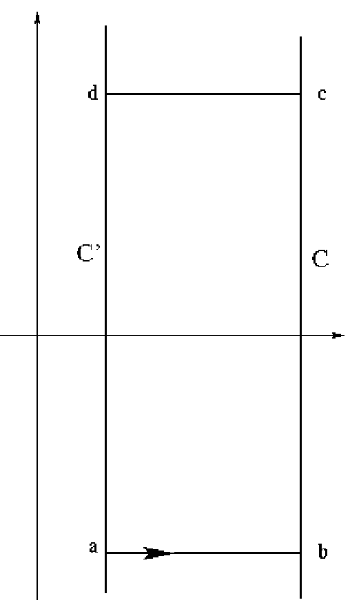
Refer to caption

Figure 3. Proof of lemma 6.3.

This lemma allows us to continue the computation, using CC instead of Ck,lC_{k,l}, provided that CC were originally chosen far enough to the right. We are about to reassemble the individual terms ∫γτσ−s​Φlk​𝑑λ\int_{\gamma_{\tau}}\sigma^{-s}\Phi^{k}_{l}d\lambda into the quantity (−∇L2)−z(-\nabla_{L}^{2})^{-z}, as promised earlier.

(54) 12​π​i∑k,l\displaystyle{\frac{1}{2\pi i}}\sum_{k,l} ∫C∫XRπ∗​(η)​trs⁡t−2​(s−l/2+k)​∫γτΓ⁡(s)​σ−s​Φlk​𝑑σ​𝑑s\displaystyle\int_{C}\int_{X_{R}}\pi^{*}(\eta)\operatorname{tr_{s}}t^{-2(s-l/2+k)}\int_{\gamma_{\tau}}\Gamma(s)\sigma^{-s}\Phi_{l}^{k}d\sigma ds
=12​π​i​∑k,l∫C∫XRπ∗​(η)​trs⁡t−2​s​∫γτΓ⁡(s)​σ−s​tl−2​k​Φlk​𝑑σ​𝑑s.\displaystyle={\frac{1}{2\pi i}}\sum_{k,l}\int_{C}\int_{X_{R}}\pi^{*}(\eta)\operatorname{tr_{s}}t^{-2s}\int_{\gamma_{\tau}}\Gamma(s)\sigma^{-s}t^{l-2k}\Phi_{l}^{k}d\sigma ds.

Recall that Φlk\Phi^{k}_{l} depends on the quantity σ=λt2\sigma={\frac{\lambda}{t^{2}}}. Also, recall (44):

(55) Φ~lk=tl−2​(k+1)​Φlk.\displaystyle\tilde{\Phi}^{k}_{l}=t^{l-2(k+1)}\Phi^{k}_{l}.

So, by (45), summing the right-hand side of (6) over ll we obtain:

(56) 12​π​i\displaystyle{\frac{1}{2\pi i}} ∑l∫C∫XRπ∗​(η)​trs⁡t−2​(s−l/2+k)​∫γτΓ⁡(s)​σ−s​Φlk​𝑑σ​𝑑s\displaystyle\sum_{l}\!\int_{C}\!\!\int_{X_{R}}\!\!\!\!\!\pi^{*}(\eta)\operatorname{tr_{s}}t^{-2(s-l/2+k)}\int_{\gamma_{\tau}}\!\!\!\!\!\Gamma(s)\sigma^{-s}\!\Phi_{l}^{k}d\sigma ds
=12​π​i​∑l∫C∫XRπ∗​(η)​trs​∫γτ​t2Γ⁡(s)​λ−s​Φ~lk​𝑑λ​𝑑s\displaystyle={\frac{1}{2\pi i}}\sum_{l}\int_{C}\int_{X_{R}}\pi^{*}(\eta)\operatorname{tr_{s}}\int_{\gamma_{\tau t^{2}}}\Gamma(s)\lambda^{-s}{\tilde{\Phi}_{l}^{k}}d\lambda ds
=12​π​i∫C∫XRπ∗(η)×trs∫γτ​t2λ−z(−1)k(λ+t2L2)−1\displaystyle=\!\!{\frac{1}{2\pi i}}\int_{C}\!\int_{X_{R}}\!\!\!\!\!\!\!\pi^{*}\!(\eta)\!\times\!\!\operatorname{tr_{s}}\!\!\int_{\gamma_{{\tau t^{2}}}}\!\!\!\!\!\!\!\lambda^{-z}(-1)^{k}(\lambda\!+t^{2}L^{2})^{\!\!{}^{-1}}
×[(λ+t2L2)−1Θt]kdλ.\displaystyle\!\qquad\qquad\qquad\qquad\qquad\qquad\times\big[(\lambda\!+t^{2}L^{2})^{\!\!{}^{-1}}\!\Theta_{t}\big]^{k}\!d\lambda.

Finally, by summing this over all kk, we recover the quantity

(57) 12​π​i​∫C∫XRπ∗​(η)​trs⁡Γ⁡(s)​(−∇t​L)−2​s​𝑑s.\displaystyle{\frac{1}{2\pi i}}\int_{C}\int_{X_{R}}\pi^{*}(\eta)\operatorname{tr_{s}}\Gamma(s)(-\nabla_{tL})^{-2s}ds.

We now invoke theorem 3.4 and lift our standing assumption that R​e​(z)≫0Re(z)\gg 0. Hence, the integral ∫XR…\int_{X_{R}}\ldots in (57) may be replaced by its meromorphic extension. We can now finish the proof, by moving the vertical CC to the left and “picking up” all the residues. The procedure is explained in the following lemma.

Lemma 6.4.

For any r>0r>0 such that (C−r)(C-r) does not intersect the real axis at any of the residues, the following holds:

(58) ∫CΓ⁡(s)​∫XRπ∗​(η)\displaystyle\int_{C}\Gamma(s)\int_{X_{R}}\pi^{*}(\eta) (−∇t​L2)−s​d​s=\displaystyle(-\nabla_{tL}^{2})^{-s}ds=
∫C−rΓ⁡(s)​∫XRπ∗​(η)​(−∇t​L2)−s​𝑑s+\displaystyle\int_{C-r}\Gamma(s)\int_{X_{R}}\pi^{*}(\eta)(-\nabla_{tL}^{2})^{-s}ds\,+
∑R​e​(s)>−rR​e​s|s​Γ​(s)​∫XRπ∗​(η)​(−∇t​L2)−s.\displaystyle\,\,\,\sum_{Re(s)>-r}Res|_{s}\Gamma(s)\int_{X_{R}}\pi^{*}(\eta)(-\nabla_{tL}^{2})^{-s}.

Further, substituting rm=2​m+12r_{m}={\frac{2m+1}{2}} instead of rr in the above expression, the integral on the right-hand side tends to zero as m→∞m\to\infty, so that

(59) ∫CΓ⁡(s)​∫XRπ∗​(η)\displaystyle\int_{C}\Gamma(s)\int_{X_{R}}\pi^{*}(\eta) (−∇t​L2)−s​d​s=\displaystyle(-\nabla_{tL}^{2})^{-s}ds=
∑s∈ℂR​e​s|s​Γ​(s)​∫XRπ∗​(η)​(−∇t​L2)−s.\displaystyle\sum_{s\in{{\mathbb{C}}}}Res|_{s}\Gamma(s)\int_{X_{R}}\pi^{*}(\eta)(-\nabla_{tL}^{2})^{-s}.

Proof: The first equation follows by the argument similar to that in lemma 6.3 (Fig. 4). Next, because of the identity z​Γ​(z)=Γ⁡(z+1)z\Gamma(z)=\Gamma(z+1), the quantity supy∈ℝ|Γ⁡(x+i​y)|\sup_{y\in{{\mathbb{R}}}}|\Gamma(x+iy)| decays superexponentially as x→−∞x\to-\infty. Therefore, by our estimate in corollary (5.4) on the integral
It​(η,z)=∫XRπ∗​(η)​(−∇t​L2)−s​𝑑sI_{t}(\eta,z)=\int_{X_{R}}\pi^{*}(\eta)(-\nabla_{tL}^{2})^{-s}ds, (59) follows. ∎

Refer to caption

Figure 4. As CC is moved to the left, we pick up the residues.

Finally, we need to prove that as R→0R\to 0, only finitely many residues survive. By theorem 3.4, It​(η,z)I_{t}(\eta,z) has only finitely many poles and they are at most simple. Also, Γ⁡(z)\Gamma(z) has at most simple poles, at z=0,−1,−2​…z=0,-1,-2\ldots. So, the residues of Γ⁡(z)​It​(η,z)\Gamma(z)I_{t}(\eta,z) are due to either one of these factors. But the theorem 3.4, provides us with some knowledge of the general algebraic form of It​(η,z)I_{t}(\eta,z). It implies that for m>>0m>>0, the residue at z=−mz=-m will be a multiple of a positive power of RR, so it will vanish as R→0R\to 0. ∎

7. The de Rham operator on Riemanian surfaces.

We consider the complexified vector bundle E⊗ℂ=Λ∗​M⊗ℂE\otimes{{\mathbb{C}}}=\Lambda^{*}M\otimes{{\mathbb{C}}} of exterior forms over a compact manifold MM with no boundary. The grading decomposition is that into differential forms of even and odd degree. Given a Riemanian metric gg on M,M, the associated de Rham operator D=d+d∗D=d+d^{*} has a well-known symbol L=−ρ2L=-\rho^{2}.

In order to apply the theorem 3.6, we need to compute:

(−(∇+L)2)−z=(−(L2+∇2+[∇,L]))−z.(-(\nabla+L)^{2})^{-z}=(-(L^{2}+\nabla^{2}+[\nabla,L]))^{-z}.

The argument of the function ν↦−ν−z\nu\mapsto-\nu^{-z} can be viewed as −ρ2-\rho^{2} plus some commuting perturbation which is nilpotent. It follows that we may just use the Taylor series expansion instead of the Cauchy integrals:

(−(∇+L)2)−z=∑k=02​n(ρ2)−(z+k)(k−(z+k))(∇2+[∇,L])k,(-(\nabla+L)^{2})^{-z}=\sum_{k=0}^{2n}(\rho^{2})^{-(z+k)}\big(_{\,\,\,\,\,\,\,\,k}^{-(z+k)}\big)(\nabla^{2}+[\nabla,L])^{k},

where (kz)\big(^{z}_{k}\big) means −z⁡(−z−1)​…​(−z−k+1)k!{\frac{-z(-z-1)\ldots(-z-k+1)}{k!}}.

For example, we consider the case when MM is a 2-manifold and η≡1\eta\equiv 1. Since that is exactly the todd class for any 2-surface, by the Atiyah-Singer index theorem both sides of theorem 3.6 should give us the euler characteristic. The left-hand side of theorem 3.6 yields:

(60) ∫T∗​Mexp⁡((CLOSECLOSE\displaystyle\int_{T^{*}M}\exp(( OPENOPEN∇+L)2)=\displaystyle\nabla+L)^{2})=
=∫T∗​Mexp⁡(−ρ2)​exp⁡(∇2+[L,∇])\displaystyle=\int_{T^{*}M}\exp(-\rho^{2})\exp(\nabla^{2}+[L,\nabla])
=∫T∗​Mexp⁡(−ρ2)​(1+(∇2+[L,∇])+12​(∇2+[L,∇])2+…)\displaystyle=\int_{T^{*}M}\exp(-\rho^{2}){\scriptstyle(1+(\nabla^{2}+[L,\nabla])+{\frac{1}{2}}(\nabla^{2}+[L,\nabla])^{2}+\ldots)}
=∫T∗​Mexp⁡(−ρ2)​(13!​(∇2+[L,∇])3+14!​(∇2+[L,∇])4)\displaystyle=\int_{T^{*}M}\exp(-\rho^{2}){\scriptstyle({\frac{1}{3!}}(\nabla^{2}+[L,\nabla])^{3}+{\frac{1}{4!}}(\nabla^{2}+[L,\nabla])^{4})}

We keep only these two terms because they are the only ones that can possibly contain a 44-form which can be integrated over T∗​M.T^{*}M. In fact, when we expand (∇2+[L,∇])3(\nabla^{2}+[L,\nabla])^{3} we see that only three terms really enter the picture, namely ∇2[L,∇]2,\nabla^{2}[L,\nabla]^{2}\,\,, [L,∇]2​∇2,[L,\nabla]^{2}\nabla^{2}, and [L,∇]​∇2[L,∇][L,\nabla]\nabla^{2}[L,\nabla]. From (∇2+[L,∇])4,(\nabla^{2}+[L,\nabla])^{4}, the relevant term is [L,∇]4.[L,\nabla]^{4}.

Lemma 7.1.

The term [L,∇]4[L,\nabla]^{4} vanishes as a section of Λ∗​T∗​M⊗E​n​d​(π∗​E)\Lambda^{*}T^{*}M\otimes End(\pi^{*}E), i.e., pointwise.
Proof: From section 5,

[L,∇]=dx​L+dξ​L+[θ,L],[L,\nabla]=d_{x}L+d_{\xi}L+[\theta,L],

If one uses normal coordinates on MM near some point xx, then θ\theta, being comprised of Christoffel symbols is zero on the fiber of T∗​MT^{*}M over xx. The horizontal differential dx​Ld_{x}L is also zero there. Hence on that fiber, [L,∇]=dξ​L[L,\nabla]=d_{\xi}L which is a matrix of “vertical” forms on T∗​MT^{*}M. Any power of it which is larger than d​i​m​(M)dim(M) must vanish.∎

Thus, the left-hand side of theorem 3.6 reads:

(61) ∫T∗​Mexp⁡(−ρ2)​16​(∇2[L,∇]2+[L,∇]2​∇2+[L,∇]​∇2[L,∇]).\int_{T^{*}M}\exp(-\rho^{2}){\frac{1}{6}}{(\nabla^{2}[L,\nabla]^{2}+[L,\nabla]^{2}\nabla^{2}+[L,\nabla]\nabla^{2}[L,\nabla])}.

Similar remarks apply on the right-hand side and we obtain:

(62) limR→0∑R​e​s|z​Γ​(z)​∫XR−z​(z+1)​(z+2)6​ρ−2​(z+3)\displaystyle\lim_{R\to 0}\sum Res|_{z}\Gamma(z)\int_{X_{R}}{\frac{-z(z+1)(z+2)}{6}}\rho^{-2(z+3)}
(∇2[L,∇]2+[L,∇]2​∇2+[L,∇]​∇2[L,∇]).\displaystyle(\nabla^{2}[L,\nabla]^{2}+[L,\nabla]^{2}\nabla^{2}+[L,\nabla]\nabla^{2}[L,\nabla]).

Since t⁡rs​(∇2[L,∇]2+[L,∇]2​∇2+[L,∇]​∇2[L,∇])=ω​ρ​d​ρ{\operatorname{t}r_{s}}{\scriptstyle(\nabla^{2}[L,\nabla]^{2}+[L,\nabla]^{2}\nabla^{2}+[L,\nabla]\nabla^{2}[L,\nabla])}=\omega\rho d\rho for some differential form ω\omega, it is enough to see that:

(63) ∫0∞e​x​p​(CLOSE\displaystyle\int_{0}^{\infty}\!\!\!\!exp( OPEN−ρ2)​ρ​d​ρ=\displaystyle-\rho^{2})\rho d\rho\!=
=limR→0∑R​e​s|z​Γ​(z)​∫R∞(−z)​(z+1)​(z+2)​ρ−2​(z+3)​ρ​𝑑ρ\displaystyle=\lim_{R\to 0}\sum Res|_{z}\Gamma(z)\int_{R}^{\infty}\!\!\!\!\!{(-z)(z+1)(z+2)}\rho^{-2(z+3)}\rho d\rho
=12​limR→0∑R​e​s|z​Γ​(z+2)​R−2​(z+2)\displaystyle={\frac{1}{2}}\lim_{R\to 0}\sum Res|_{z}\Gamma(z+2)R^{-2(z+2)}
=12​limR→0∑m=0∞(−1)mm!​R2​m.\displaystyle={\frac{1}{2}}\lim_{R\to 0}\sum_{m=0}^{\infty}{\frac{(-1)^{m}}{m!}}R^{2m}.

8. The Chern character for a general spinor bundle.

We apply our results to the Chern character of a spinor bundle S→MS\to M associated to a vector bundle π:F→M\pi\colon\thinspace F\to M, as computed by Mathai and Quillen [10]. The role of the cotangent bundle π:T∗​M→M\pi\colon\thinspace T^{*}M\to M is played by FF in this example, and the role of E→ME\to M is played by SS. So, theorem 3.6, strictly speaking does not apply, though we could have proven it in a more general setting. The reason we stated our theorem for T∗​MT^{*}M is that we have the Atiyah-Singer index theorem in mind, for future applications. Rather than applying theorem 3.6, we will go through its proof. Namely, we shall repeat steps (2) and (3) in a simpler way.

We proceed to outline the result of [10]. Some familiarity with spin structures is assumed here. The reader can consult, e.g., Spin Geometry by Lawson and Michelsohn for details [9]. We also warn that the notation of [10] is quite a bit different from our own. We will briefly explain the differences in the end of this section.

Let π:F→M\pi\colon\thinspace F\to M be a complex even-dimensional vector bundle with a spin structure. In particular, this means that there is a fiberwise metric μ\mu on FF. Let S→MS\to M be the associated spinor bundle. The assumption of spin structure implies that SS can be split into a direct sum of even and odd subbundles: S=S+⊕S−S=S^{+}\oplus S^{-}, where the fibers Sx+S_{x}^{+} and Sx−S_{x}^{-} of S+S^{+} and S−S^{-} are the only two irreducible representations for the spin group of the fiber FxF_{x}. Thus, the spin structure induces a ℤ2{{\mathbb{Z}}}_{2}-grading of SS.

In order to form a Chern character we need a connection ∇′\nabla^{\prime} on SS which respects that ℤ2{{\mathbb{Z}}}_{2}-grading. We also need an odd antiselfadjoint endomorphism LL of π∗​S\pi^{*}S. The spinor bundle setup in [10] requires, among other things, that:

  • •

    LL be homogeneous of degree 1 in the radial coordinate ρ\rho of the fibers of FF. Much as in the proof of theorems 3.4 and 3.6, ρ\rho is induced by the metric μ\mu and is given by ρ⁡(p)=μ⁡(p,p)\rho(p)=\sqrt{\mu(p,p)} for all pp in FF.

  • •

    ∇′\nabla^{\prime} preserve the fiberwise metric (⋅,⋅)(\cdot,\cdot) which is induced on SS by the metric μ\mu of FF. This means that for any two sections α\alpha and β\beta of SS,

    d⁡(α,β)=(∇′α,β)+(α,∇′β).d(\alpha,\beta)=(\nabla^{\prime}\alpha,\beta)+(\alpha,\nabla^{\prime}\beta).

The coordinate notation is the same as in the proof of theorem 3.4. The local coordinates on FF are the vertical (fiberwise) cartesian coordinates are ξ1,…,ξm\xi^{1},\ldots,\xi^{m}, and the horizontal coordinates x1,…​xnx_{1},\ldots x_{n}, which are also coordinates of MM. In fact, it makes sense to choose the μ\mu-orthonormal local frame e1,…​eme_{1},\ldots e_{m} of FF and to choose coordinates ξj\xi^{j} associated to that frame. They may be replaced by spherical coordinates ρ\rho and Ξ1,…,Ξm−1\Xi^{1},\ldots,\Xi^{m-1} at our convenience.

To describe LL we recall that the spin structure of FF stems from the fiberwise metric μ\mu. To begin with, we have the Clifford action of FF on SS which is a fiberwise ℝ{{\mathbb{R}}}-linear bundle map c:F→E​n​d​(S),c\colon\thinspace F\to End(S), such that for any (x,ξ)(x,\xi) in FxF_{x}, c​(x,ξ)2=−μx​(ξ,ξ)c(x,\xi)^{2}=-\mu_{x}(\xi,\xi). It is one of the standard axioms for a Clifford actions that c⁡(x,ξ)c(x,\xi) be fiberwise anti-selfadjoint endomorphism. Thus, each fiber FxF_{x} is contained in a clifford algebra C​l​i​f​f​(Fx,μx)Cliff(F_{x},\mu_{x}), which is a fiber of the bundle C​l​i​f​f​(F,μ)Cliff(F,\mu). Also, there is a map

C​l​i​f​f​(F,μ)→E​n​d​(S),Cliff(F,\mu)\to End(S),

which is an isomorphism of bundles and fiberwise an isomorphism of algebras. Now, the pullback π∗​F\pi^{*}F to the total space of FF is equipped with the Clifford action on π∗​S\pi^{*}S which we shall also denote cc instead of π∗​c\pi^{*}c. Let τ:F→π∗​F\tau\colon\thinspace F\to\pi^{*}F be the tautological section. Then the endomorphism L=c⁡(τ⁡(x,ξ))L=c(\tau(x,\xi)) has all the required properties. Its homogeneity in ρ\rho is obvious and it is antiselfadjoint by hypothesis.

Abbreviating c⁡(τ⁡(ej))c(\tau(e_{j})) by γj\gamma_{j}, we may write L=∑jξj​γjL=\sum_{j}\xi^{j}\gamma_{j}. Since the construction of the clifford action on spinors using an orthonormal basis is completely canonical, the coordinate expression for LL does not involve the xx-variables. Since,

12​(γi​γj+γj​γi)=−δi​j,{\frac{1}{2}}(\gamma_{i}\gamma_{j}+\gamma_{j}\gamma_{i})=-\delta_{ij},

it follows that L2=μ⁡(ξ,ξ)=−ρ2L^{2}=\mu(\xi,\xi)=-\rho^{2}.

Next, to pick a connection on ∇′\nabla^{\prime}, we start with a connection on FF which is locally given by d+θd+\theta. The connection ∇′\nabla^{\prime} on SS is constructed from it (see [10] and [9]). In order to describe the construction, we adopt the summation notation: we reserve the right to write any index as an upper or a lower index. (Since we have chosen an orthonormal local frame, there is no difference at all). Repetition of the same index on the top and on the bottom implies summation. Repetition on the top only or on the bottom only does not. The connection on π∗​S\pi^{*}S is given by

∇′=d+14​θi​j​γi​γj,\nabla^{\prime}=d+{\frac{1}{4}}\theta^{ij}\gamma_{i}\gamma_{j},

where θi​j\theta^{ij} are just the matrix entries of the endomorphism-valued11-form θ\theta. The connection ∇=π∗​∇′\nabla=\pi^{*}\nabla^{\prime} on π∗​S\pi^{*}S therefore makes sense. Observe that since γj\gamma_{j} are odd, the local endomorphism θi​j​γi​γj\theta^{ij}\gamma_{i}\gamma_{j} of π∗​S\pi^{*}S is even. Moreover, it only depends on the variables xix_{i} and horizontal differentials d​xidx_{i}, just as before. Therefore, the curvature of the connection ∇L\nabla_{L} may be written as:

(64) ∇L2\displaystyle\nabla_{L}^{2} =∇2+[∇,L]−ρ2\displaystyle=\nabla^{2}+[\nabla,L]-\rho^{2}
=∇2+d​ξj​γj+ξk4​[θi​j​γi​γj,γk]−ρ2\displaystyle=\nabla^{2}+d\xi^{j}\gamma_{j}+{\frac{\xi^{k}}{4}}[\theta^{ij}\gamma_{i}\gamma_{j},\gamma_{k}]-\rho^{2}
=∇2+(d​ξj)​γj+ξj4​θi​j​γi−ρ2\displaystyle=\nabla^{2}+(d\xi^{j})\gamma_{j}+{\frac{\xi^{j}}{4}}\theta^{ij}\gamma_{i}-\rho^{2}

Here, just as in the previous example, the fact that L2L^{2} is a scalar is a tremendous simplification. We may use Taylor series instead of Cauchy integrals and we have the rule ea+b=ea​eb.e^{a+b}=e^{a}e^{b}.

Now, the result from [10] reads:

(65) trs⁡exp⁡∇L2\displaystyle\operatorname{tr_{s}}\exp\nabla^{2}_{L} =(−1)m/2(i2​π)−m/2det(sinh⁡(∇2/2)(∇2/2))12\displaystyle=(-1)^{m/2}\Big({\frac{i}{2\pi}}\Big)^{-m/2}\det\left({\frac{\sinh(\nabla^{2}/2)}{(\nabla^{2}/2)}}\right)^{\frac{1}{2}}
×trs(π−m/2e−ρ2∑Iε(I,I′)Pf(∇2/2)I∏j∈I′((dξj)γj+ξj4θjiγi)),\displaystyle\,\,\qquad\times\operatorname{tr_{s}}({\scriptstyle\pi^{-m/2}e^{-\rho^{2}}\sum_{I}\varepsilon(I,I^{\prime})Pf(\nabla^{2}/2)_{I}\prod_{j\in I^{\prime}}((d\xi_{j})\gamma_{j}+{\frac{\xi^{j}}{4}}\theta^{i}_{j}\gamma_{i})}),

where:

  • •

    I,I′I,I^{\prime} are complementary (strictly increasing) multiindices over the set {1,2,…​m}\{1,2,\ldots\,m\} and ε⁡(I,I′)\varepsilon(I,I^{\prime}) is a certain combinatorial ±1\pm 1-valued function of them, which shall not be relevant here.

  • •

    P​f​(∇2/2)IPf(\nabla^{2}/2)_{I} is the Pfaffian of the submatrix of ∇2/2\nabla^{2}/2 determined by the multiindex II. For an unfamiliar reader, it suffices to know that it is a certain polynomial in the matrix entries of ∇2\nabla^{2} which is just 11 if II is the empty multiindex.

For us, (65) is greatly simplified by the fact that we are only interested in the currents induced by this Chern character on Ω∗​M\Omega^{*}M. Therefore, as observed in theorem 3.4 and lemma 3.5, we need only those terms of (65) which involve all the differentials d​ξjd\xi^{j}, so the only relevant multiindex is I′=(1,2,…,m)I^{\prime}=(1,2,\ldots,m), II being empty and P​f​(∇2/2)IPf(\nabla^{2}/2)_{I} being 11. The only term of interest is therefore

π−m/2e−ρ2dξ1…dξm.\pi^{-m/2}e^{-\rho^{2}}d\xi^{1}\ldots d\xi^{m}.

If we replace LL by t​LtL, as in theorem 3.6, (65) becomes

(66) trs⁡exp⁡∇L2\displaystyle\operatorname{tr_{s}}\exp\nabla^{2}_{L} =(−1)m/2(i2​π)−m/2det(sinh⁡(∇2/2)(∇2/2))12\displaystyle=(-1)^{m/2}\Big({\frac{i}{2\pi}}\Big)^{-m/2}\det\left({\frac{\sinh(\nabla^{2}/2)}{(\nabla^{2}/2)}}\right)^{\frac{1}{2}}
×trstmπ−m/2e−t2​ρ2dξ1…dξm.\displaystyle\qquad\qquad\qquad\times\operatorname{tr_{s}}t^{m}\pi^{-m/2}e^{-t^{2}\rho^{2}}d\xi^{1}\ldots d\xi^{m}.

Integrating this over any fiber of FF, we see that for any η∈Ω∗​M\eta\in\Omega^{*}M,

(67) ∫Fπ∗​(η)​trs\displaystyle\int_{F}\pi^{*}(\eta)\operatorname{tr_{s}} exp⁡∇L2=\displaystyle\exp\nabla^{2}_{L}=
∫Fπ∗(η)(−1)m/2(i2​π)−m/2det(sinh⁡(∇2/2)(∇2/2))12.\displaystyle\int_{F}\pi^{*}(\eta)(-1)^{m/2}\Big({\frac{i}{2\pi}}\Big)^{-m/2}\det\left({\frac{\sinh(\nabla^{2}/2)}{(\nabla^{2}/2)}}\right)^{\frac{1}{2}}.

This allows us to understand the residue formulation of this Chern character.

A computation similar to the one in the previous example yields:

(68) exp⁡∇L2\displaystyle\exp\nabla^{2}_{L} =∑k,l12​π​i∫C(kz)Γ(z)ρ−2​(z+k)Pk−l,l(∇2,[∇,L])dz,\displaystyle=\sum_{k,l}{\frac{1}{2\pi i}}\int_{C}\!\!\!\!\big(^{z}_{k}\big)\Gamma(z)\rho^{-2(z+k)}{P_{k-l,l}(\nabla^{2},[\nabla,L])}dz,

where by Pμ,ν​(A,B)P_{\mu,\nu}(A,B) we denote the homogeneous non-commutative polynomial in AA and BB obtained by summing all the words comprised of μ\mu copies of AA and ν\nu copies of BB.

We now recall (65). It involves the sum over multiindices I′I^{\prime} and the only relevant multiindex was determined to be I′=(1,2​…,m)I^{\prime}=(1,2\ldots\,,m), where mm is the fiberwise dimension of FF. This means that in (68) only the terms with l=ml=m contribute to the current induced by Chern character on Ω∗​M\Omega^{*}M. We have seen a special case of this in the previous example, where a normal coordinates argument was used to show that only the terms which involve two copies of [∇,L][\nabla,L] are relevant. (Recall from lemma 3.5 that such terms were called contributing.) In particular, it means that [∇,L][\nabla,L] contributes the vertical differentials and no other differentials.

Coming back to our computation, the right-hand side of (68) is readily seen to be the Taylor series for Γ⁡(z)​(−∇L2)−2​z\Gamma(z)(-\nabla^{2}_{L})^{-2z}. The discussion in the previous paragraph implies that the contributing part of Pk−l,l​(∇2,[∇,L])P_{k-l,l}(\nabla^{2},[\nabla,L]) is a multiple of the vertical volume form:

d​ξ1​…​d​ξm=ρm−1​d​ρ​d​Ξ1​…​d​ξm−1.d\xi^{1}\ldots d\xi^{m}=\rho^{m-1}d\rho d\Xi^{1}\ldots d\xi^{m-1}.

Thus, it supplies m−1m-1 powers of ρ\rho. It remains to determine the residues, using the procedure from theorem 3.4. Just as in that theorem, we set

XR=d​e​f{p∈F:ρ(p)≥R},X_{R}=_{{}_{def}}\{p\in F\colon\thinspace\rho(p)\geq R\},

and integrate from RR to ∞\infty with respect to ρ\rho. This, as we shall see, produces the residue at (m−2​k)/2(m-2k)/2. Let η∈Ωκ​M\eta\in\Omega^{\kappa}M, and express (−∇L2)−z(-\nabla^{2}_{L})^{-z} as a sum of two differential forms:

(−∇L2)−z=νz+ωz​d​ρ,(-\nabla^{2}_{L})^{-z}=\nu_{z}+\omega_{z}d\rho,

where neither νz\nu_{z} nor ωz\omega_{z} involve d​ρd\rho. We obtain:

(69) Γ⁡(z)​∫XRπ∗​(η)​(−∇L2)−z\displaystyle\Gamma(z)\int_{X_{R}}\pi^{*}(\eta)(-\nabla^{2}_{L})^{-z} =∫R∞ρ−2​(z+k)+m−1​𝑑ρ​∫S∗​Mπ∗​(η)​ωz\displaystyle=\int_{R}^{\infty}\rho^{-2(z+k)+m-1}d\rho\int_{S^{*}M}\pi^{*}(\eta)\omega_{z}
=R−2​(z+k)+m2​(z+k)+m​∫S∗​Mπ∗​(η)​ωz.\displaystyle={\frac{R^{-2(z+k)+m}}{2(z+k)+m}}\int_{S^{*}M}\pi^{*}(\eta)\omega_{z}.

Counting the differential form degrees, we see that if deg⁡(η)=κ\deg(\eta)=\kappa, then the only contributing term of (68) is the (k,m)(k,m)-th term. Here kk satisfies 2​k−m=m+n−κ2k-m=m+n-\kappa. This term produces a residue at m/2−km/2-k which is a current on κ\kappa- forms. But according to (67), the same current is induced by the (n−κ)(n-\kappa)-component of the differential form det(sinh⁡(∇2/2)(∇2/2))12\det\left({\frac{\sinh(\nabla^{2}/2)}{(\nabla^{2}/2)}}\right)^{\frac{1}{2}}, so that:

∫Mηdet\displaystyle\int_{M}\eta\det (sinh⁡(∇2/2)(∇2/2))n−κ12=\displaystyle\left({\frac{\sinh(\nabla^{2}/2)}{(\nabla^{2}/2)}}\right)^{\frac{1}{2}}_{n-\kappa}=
limR→0R​e​s|κ−m−n2​(Γ⁡(z)​∫XRπ∗​(η)​trs⁡(−∇L2)−z),\displaystyle\lim_{R\to 0}Res|_{\frac{\kappa-m-n}{2}}\left(\Gamma(z)\int_{X_{R}}\pi^{*}(\eta)\operatorname{tr_{s}}(-\nabla_{L}^{2})^{-z}\right),

which agrees with lemma 3.5 if m=nm=n.

Remark 8.1.

The condition 2​k−m=m+n−κ2k-m=m+n-\kappa implies that we only have nonzero currents on κ\kappa forms if κ\kappa is of the same parity as nn. Thus, the location of the residue is an integer if mm is even and a half-integer if mm is odd.

Warning: In [10], the relevant computation is in section 4, where FF is denoted by EE, ∇2\nabla^{2} is denoted by Ω\Omega and the fiberwise coordinates ξj\xi^{j} are denoted by xjx^{j}.

References

  • [1] G. Arfken. Mathematical Methods for Physicists, 3rd ed. Academic Press, 1985.
  • [2] M. F. Atiyah and I. M. Singer. The index of elliptic operators on compact manifolds. Bull. Amer. Math. Soc., 69:322–433, 1963.
  • [3] M. F. Atiyah and I. M. Singer. The index of elliptic operators i, ii, iii. Ann. Math., 87:484–604, 1968.
  • [4] M. F. Atiyah and I. M. Singer. The index of elliptic operators iv. Ann. Math., 93:119–138, 1971.
  • [5] A. Connes. Noncommutative differential geometry. IHES Publ. Math., (62), 1985.
  • [6] A. Connes. Noncommutative geometry. Academic Press, 1994.
  • [7] A. Connes and H. Moscovici. The local index formula in noncommutative geometry. Geometric and Functional Analysis, 5(2):174–243, 1995.
  • [8] J. M. Gracia-Bondia; J. C. Varilly; H. E. Figueroa. Elements of noncommutative geometry. Birkha̋user Advanced Texts: Basler Lehrbűcher, 2001.
  • [9] H. B. Lawson and M. Michelsohn. Spin Geometry. Princeton University Press, 1990.
  • [10] V. Mathai and D. Quillen. Superconnections thom classes and equvariant differential forms. Topology, 25(1):85–110, 1986.
  • [11] D. Quillen. Algebra cochains and cyclic cohomology. Publ. Math. I.H.E.S., 68:139–174, 1984.
  • [12] D. Quillen. Superconnections and the chern character. Topology, 24(1):89–95, 1985.