Painlevé formulas of the limiting distributions for non-null complex sample covariance matrices

Jinho Baik Note: Department of Mathematics, University of Michigan, Ann Arbor, MI, 48109, baik@umich.edu Note: 2000 Mathematics Subject Classification: 33E17, 60E99, 62E99

July 20, 2005

Abstract

In a recent study of large non-null sample covariance matrices, a new sequence of functions generalizing the GUE Tracy-Widom distribution of random matrix theory was obtained. This paper derives Painlevé formulas of these functions and use them to prove that they are indeed distribution functions. Applications of these new distribution functions to last passage percolation, queues in tandem and totally asymmetric simple exclusion process are also discussed. As a part of the proof, a representation of orthogonal polynomials on the unit circle in terms of an operator on a discrete set is presented.

1 Introduction

Let $\Ai(u)$ denote the Airy function. It has an integral representation

\Ai(u)=\frac{1}{2\pi}\int e^{i(ua+\frac{1}{3}a^{3})}da

(1.1)

where the integral is over a curve from $\infty e^{5i\pi/6}$ to $\infty e^{i\pi/6}$ . The Airy kernel (see, e.g. [13, 27]) is defined as

\mathbf{A}(u,v):=\frac{\Ai(u)\Ai^{\prime}(v)-\Ai(u)\Ai^{\prime}(v)}{u-v}=\int_{0}^{\infty}\Ai(u+z)\Ai(z+v)dz.

(1.2)

Let $\mathbf{A}_{x}$ be the Airy operator acting on $L^{2}((x,\infty))$ whose kernel is given by $\mathbf{A}(u,v)$ . Define

F_{0}(x):=\det\bigl(1-\mathbf{A}_{x}\bigr).

(1.3)

The ‘GUE Tracy-Widom distribution function’ $F_{0}(x)$ is the limiting distribution function of various models in mathematical physics, probability and statistics (see e.g. [28] and references in it).¹¹ 1 In many literatures, $F_{0}$ is denoted by $F_{2}$ . In this paper, we reserve $F_{2}$ for a different function. Especially in statistics, the largest eigenvalue of the sample covariance matrix of complex Gaussian samples with the identity covariance (the so-called null case) is known to have the limiting distribution given by $F_{0}(x)$ . An intriguing result by Tracy and Widom [27] is that the Fredholm determinant has an alternative expression:

F_{0}(x)=\det\bigl(1-\mathbf{A}_{x}\bigr)=\exp\biggl(-\int_{x}^{\infty}(s-x)u^{2}(s)ds\biggr),

(1.4)

where $u(x)$ is the solution to the Painlevé II equation

u^{\prime\prime}=2u^{3}+xu,

(1.5)

subject to the condition

u(x)\sim-\Ai(x)\qquad\text{as $x\to+\infty$}.

(1.6)

It is known [17] that there is a unique global solution to the equation (1.5) with the condition (1.6), and the solution satisfies (see, e.g. [17, 10])

	$\displaystyle u(x)$	$\displaystyle=$	$\displaystyle-\Ai(x)+O\biggl(\frac{e^{-\frac{1}{4}x^{3/2}}}{x^{1/4}}\biggr),\qquad x\to+\infty$		(1.7)
	$\displaystyle u(x)$	$\displaystyle=$	$\displaystyle-\sqrt{\frac{-x}{2}}\biggl(1+O\biggl(\frac{1}{x^{2}}\biggr)\biggr),\qquad x\to-\infty.$		(1.8)

Recall that $\Ai(x)\sim e^{-\frac{2}{3}x^{3/2}}/(2\sqrt{\pi}x^{1/4})$ as $x\to+\infty$ . The right-hand-side of (1.4) provides a practical formula to plot the graph of $F_{0}$ numerically.

For $m=1,2,3,\dots$ and for complex numbers $w_{1},w_{2},\dots$ , define

s^{(m)}(u;w_{1},\dots,w_{m})=s^{(m)}(w_{1},\dots,w_{m}):=\frac{1}{2\pi}\int e^{\frac{1}{3}ia^{3}+iua}\prod_{j=1}^{m}\frac{1}{w_{j}+ia}da

(1.9)

where the contour is from $\infty e^{5i\pi/6}$ to $\infty e^{i\pi/6}$ such that the poles $a=iw_{1},\dots,iw_{m}$ lie above the contour. Also define

t^{(m)}(v;w_{1},\dots,w_{m-1})=t^{(m)}(w_{1},\dots,w_{m-1}):=\frac{1}{2\pi}\int e^{\frac{1}{3}ib^{3}+ivb}\prod_{j=1}^{m-1}(w_{j}-ib)db

(1.10)

where the contour is from $\infty e^{5i\pi/6}$ to $\infty e^{i\pi/6}$ . Comparing with (1.1), $t^{(m)}$ is a sum of derivatives of the Airy function. On the other hand, when $w_{1}=\dots=w_{m}=0$ , $s^{(m)}$ is a sum of anti-derivatives of the Airy function. However for general $w_{j}$ ’s, $s^{(m)}$ is a Cauchy-type transform of the integrand of the Airy function. Define

\begin{split}&F_{k}(x;w_{1},\dots,w_{k})\\ &\quad:=F_{0}(x)\cdot\det\biggl(\delta_{mn}-<\frac{1}{1-\mathbf{A}_{x}}s^{(m)}(w_{1},\dots,w_{m}),t^{(n)}(w_{1},\dots,w_{n-1})>_{L^{2}((x,\infty))}\biggr)_{1\leq m,n\leq k}\end{split}

(1.11)

where $<,>_{(x,\infty)}$ denotes the real inner product in $L^{2}((x,\infty))$ ;

\begin{split}&<\frac{1}{1-\mathbf{A}_{x}}s^{(m)}(w_{1},\dots,w_{m}),t^{(n)}(w_{1},\dots,w_{n-1})>_{L^{2}((x,\infty))}\\ &\qquad=\int_{x}^{\infty}\biggl(\frac{1}{1-\mathbf{A}_{x}}s^{(m)}(w_{1},\dots,w_{m})\biggr)(u)t^{(n)}(u;w_{1},\dots,w_{n-1})du.\end{split}

(1.12)

(It is well-known that $1-\mathbf{A}_{x}$ is invertible.) Set

F_{k}(x):=F_{k}(x;0,0\dots,0),\qquad k=1,2,\dots.

(1.13)

The functions $F_{k}(x;w_{1},\dots,w_{k})$ were introduced recently in [1] as limits of the distribution functions of the largest eigenvalues of certain non-null complex sample covariance matrices and also other probability models. See Section 2 below for more details on the motivations. The purpose of this paper is to find a Painlevé type formula for $F_{k}(x;w_{1},\cdots,w_{k})$ analogous to (1.4). Such formula is used to prove that $F_{k}(x;w_{1},\cdots,w_{k})$ is indeed a distribution. It also allows us to be able to plot the graph of $F_{k}(x)$ .

1.1 Results

1.1.1 Alternative determinantal formula

We first obtain an alternative determinantal formula of $F_{k}(x;w_{1},\dots,w_{k})$ . The definition (1.11) involves the functions $s^{(m)}$ and $t^{(m)}$ and it is not transparent that the formula is symmetric in $w_{1},\dots,w_{k}$ , which should be the case from its origin in the sample covariance matrix [1] (see also Section 2 below). This symmetry is clear in the following theorem.

For a complex number $w$ , set

C_{w}(u):=\frac{1}{2\pi}\int e^{i(\frac{1}{3}a^{3}+ua)}\frac{1}{w+ia}da

(1.14)

where the contour is, as in the definition (1.9) of $s^{(m)}$ , from $\infty e^{5i\pi/6}$ to $\infty e^{i\pi/6}$ such that the pole $a=iw$ lies above the contour. Hence $s^{(1)}(u;w_{1})=C_{w_{1}}(u)$ . Also note that $t^{(1)}(v)=\Ai(v)$ .

Theorem 1.1.

With above notations, for real $x$ and complex $w$ set

f(x,w):=1-<\frac{1}{1-\mathbf{A}_{x}}C_{w},\Ai>_{L^{2}((x,\infty))}=1-\int_{x}^{\infty}\biggl(\frac{1}{1-\mathbf{A}_{x}}C_{w}\biggr)(u)\Ai(u)du.

(1.15)

For distinct complex numbers $w_{1},\dots,w_{k}$ ,

\begin{split}F_{k}(x;w_{1},\dots,w_{k})=F_{0}(x)\cdot\frac{\det\begin{pmatrix}(w_{m}+D_{x})^{n-1}f(x,w_{m})\end{pmatrix}_{1\leq m,n\leq k}}{\displaystyle\prod_{1\leq m<n\leq k}(w_{n}-w_{m})}\end{split}

(1.16)

where $D_{x}=\frac{\partial}{\partial x}$ denotes the derivative with respect to $x$ . When some of $w_{j}$ ’s coincide, the above formula still holds by using the l’Hosptial’s rule for the right-hand-side of (3.1).

Remark.

P. Deift and A. Its pointed out that this formula resembles the Darboux transformation in the theory of integrable systems (see e.g., [23]). It would be interesting to identify the above formula in terms of a Darboux transformation of an integrable system.

This theorem follows from row and column operations of (1.11) exploiting the fact that $t^{(n)}$ is a sum of derivatives of $\Ai$ and that $s^{(m)}$ is a linear combination of $C_{w_{j}}$ . The proof is given in Section 3.

1.1.2 Painlevé formula

In the next theorem, we show that the function $f(x,w)$ defined in (1.15) is related to the Painlevé II equation.

First we need a definition. Let $M(z;x)=\biggl(\begin{smallmatrix}M_{11}(z)&M_{12}(z)\\ M_{21}(z)&M_{22}(z)\end{smallmatrix}\biggr)$ be the $2\times 2$ matrix-valued solution to the following Riemann-Hilbert problem:

•

$M(z;x)$ is analytic for $z\in\mathbb{C}\setminus\mathbb{R}$ and is continuous for $z\in\overline{\mathbb{C}\setminus\mathbb{R}}$

•

For $z\in\mathbb{R}$ ,

M_{+}(z;x)=M_{-}(z;x)\begin{pmatrix}1&-e^{-2i(\frac{4}{3}z^{3}+xz)}\\ e^{2i(\frac{4}{3}z^{3}+xz)}&0\end{pmatrix}

(1.17)

where $M_{+}(z;x)$ (resp. $M_{-}(z;x)$ ) denotes the limit of $M(z^{\prime};x)$ as $z^{\prime}\to z$ from the bottom (resp. top) of the contour $\mathbb{R}$ .

•

$M(z;x)\to I$ as $z\to\infty$ .

The precise statement of the last condition is the following: there is $\epsilon>0$ such that $M(z;x)=I+O(z^{-1})$ uniformly as $z\to\infty$ for $z$ in sectors $\epsilon<Arg(z)<\pi-\epsilon$ and $\pi+\epsilon<Arg(z)<2\pi-\epsilon$ , and $M(z;x)$ is bounded for all $z\in\mathbb{C}\setminus\mathbb{R}$ .

This is the Riemann-Hilbert problem for the Painlevé II equation when the so-called monodromy data satisfies $p=-q=1$ and $r=0$ [18, 11, 10]. It is known that there is a unique solution to this Riemann-Hilbert problem. Moreover, as $z\to\infty$ , there is an expansion of form

M(z;x)=I+\frac{M_{1}(x)}{z}+O\biggl(\frac{1}{z^{2}}\biggr),\qquad M_{1}(x)=\frac{1}{2i}\begin{pmatrix}-v(x)&u(x)\\ -u(x)&v(x)\end{pmatrix}

(1.18)

where $u(x)$ is the solution of the Painlevé II equation (1.5) satisfying (1.6), and

v(x)=\int_{\infty}^{x}u(s)^{2}ds.

(1.19)

The following theorem shows that $f(x,w)$ is expressible in terms of the Riemann-Hilbert problem for Painlevé II equation.

Theorem 1.2.

The function $f(x,w)$ defined in (1.15) satisfies the following:

f(x,w)=\begin{cases}M_{22}(-\frac{1}{2}iw;x),\qquad&Re(w)>0\\ -M_{21}(-\frac{1}{2}iw;x)e^{\frac{1}{3}w^{3}-xw},\qquad&Re(w)<0.\end{cases}

(1.20)

Note that from the jump condition (1.17), $f(x,w)$ is continuous for $w\in\mathbb{R}$ , and hence is an entire function in $w$ .

Together with Theorem 1.1, Theorem 1.2 yields the desired Painlevé II formula of $F_{k}(x;w_{1},\dots,w_{k})$ , which is the main result of this paper.

Corollary 1.3.

The function $F_{k}(x;w_{1},\dots,w_{k})$ defined by (1.11) is equal to (1.16) with $f(x,w)$ given by (1.20).

The function given in the right-hand-side of (1.20) had previously appeared in [4] (equation (2.22)) and [3] (equation (3.5)) as a limiting function for a last passage site percolation model. In the context of symmetrized random permutations and last passage percolation models, [4, 3] showed, among other things, the $k=1$ case of Corollary 1.3;

F_{1}(x,w_{1})=F_{0}(x)f(x,w_{1})

(1.21)

where $f(x,w)$ given by the right-hand-side of (1.20). This paper proves that the general case is expressible in terms of derivatives of the same function $f(x,w)$ .

1.1.3 Properties of $f(x.w)$

The papers [4, 3] proved several properties of the function defined by the right-hand-side of (1.20). By setting $w\mapsto\frac{1}{2}w$ in Lemma 2.1 of [4] or Lemma 3.1 of [3], we find the following properties of $f(x,w)$ . The following complementary function is useful: set

g(x,w):=\begin{cases}M_{12}(-\frac{1}{2}iw;x),\qquad&Re(w)>0\\ -M_{11}(-\frac{1}{2}iw;x)e^{\frac{1}{3}w^{3}-xw},\qquad&Re(w)<0.\end{cases}

(1.22)

Lemma 1.4 ([4, 3]).

The following holds.

(i).

$f(x,w),g(x,w)$ are real for $w\in\mathbb{R}$ .

(ii).

For each fixed $w\in\mathbb{C}$ , as $x\to+\infty$

	$\displaystyle f(x,w)$	$\displaystyle=$	$\displaystyle 1+O(e^{-cx^{3/2}}),$		(1.23)
	$\displaystyle g(x,w)$	$\displaystyle=$	$\displaystyle-e^{\frac{1}{3}w^{3}-xw}\bigl(1+O(e^{-cx^{3/2}})\bigr)$		(1.24)

and as $x\to-\infty$ ,

	$\displaystyle f(x,w)$	$\displaystyle\sim$	$\displaystyle\frac{1}{\sqrt{2}}e^{\frac{1}{6}w^{3}-\frac{1}{6}\|x\|^{3/2}+\frac{1}{2}\|x\|w-w^{2}\|x\|^{1/2}}$		(1.25)
	$\displaystyle g(x,w)$	$\displaystyle\sim$	$\displaystyle-\frac{1}{\sqrt{2}}e^{\frac{1}{6}w^{3}-\frac{1}{6}\|x\|^{3/2}+\frac{1}{2}\|x\|w-w^{2}\|x\|^{1/2}}.$		(1.26)

(iii).

$\displaystyle\lim_{w\to+\infty}f(x,w)=1,$	$\displaystyle\lim_{w\to+\infty}g(x,w)=0,$	(1.27)
$\displaystyle\lim_{w\to-\infty}f(x,w)=0,$	$\displaystyle\lim_{w\to-\infty}g(x,w)=0,$	(1.28)
$\displaystyle f(x,0)=\mathcal{E}(x),$	$\displaystyle g(x,0)=-\mathcal{E}(x),$	(1.29)

where

\mathcal{E}(x):=\exp\biggl\{\int_{x}^{\infty}u(s)ds\biggr\}.

(1.30)

( $\mathcal{E}(x)$ was denoted by $E(x)^{2}$ in [4, 3].)

(iv).

For all $x\in\mathbb{R}$ and $w\in\mathbb{C}$ ,

	$\displaystyle\frac{\partial}{\partial x}\binom{f(x,w)}{g(x,w)}$	$\displaystyle=$	$\displaystyle\begin{pmatrix}0&u(x)\\ u(x)&-w\end{pmatrix}\binom{f(x,w)}{g(x,w))},$		(1.31)
	$\displaystyle\frac{\partial}{\partial w}\binom{f(x,w)}{g(x,w)}$	$\displaystyle=$	$\displaystyle\begin{pmatrix}(u(x))^{2}&-wu(x)-u^{\prime}(x)\\ -wu(x)+u^{\prime}(x)&w^{2}-x-(u(x))^{2}\end{pmatrix}\binom{f(x,w)}{g(x,w)}.$		(1.32)

(v).

	$\displaystyle f(x,w)$	$\displaystyle=$	$\displaystyle-g(x,-w)e^{\frac{1}{3}w^{3}-xw},$		(1.33)
	$\displaystyle g(x,w)$	$\displaystyle=$	$\displaystyle-f(x,-w)e^{\frac{1}{3}w^{3}-xw}.$		(1.34)

(vi).

For each fixed $y\in\mathbb{R}$ , as $w\to-\infty$ ,

	$\displaystyle f(y\sqrt{\|w\|}+w^{2},w)$	$\displaystyle\to$	$\displaystyle\erf(y)=\frac{1}{\sqrt{2\pi}}\int_{-\infty}^{y}e^{-\frac{1}{2}s^{2}}ds,$		(1.35)
	$\displaystyle g(y\sqrt{\|w\|}+w^{2},w)$	$\displaystyle\sim$	$\displaystyle-e^{\frac{2}{3}\|w\|^{3}+\sqrt{2}y\|w\|^{3/2}}.$		(1.36)

Note that (1.31) and (1.32) are the Lax pair equations for the Painlevé II equation. Hence Theorem 1.1, Theorem 1.2 and Lemma 1.4 yields that $F_{k}(x;w_{1},\dots,w_{k})$ is expressible in terms of the Lax pair equations of the Painlevé II equation.

Remark.

After this paper was completed, Harold Widom found a different proof of (1.31) and (1.32) for $f(x,w)$ defined by (1.15) and $g(x,w)$ defined by $g(x,w)=-\bigl(\frac{1}{1-\mathbf{A}_{x}}C_{w}\bigr)(x)$ using the method of [27]. The proof of Widom is algebraic and is more direct. On the other hand, the current paper proves a general identity and then takes a limit as outlined in subsection 1.2 below.

From (1.31) and (1.32), $f(x,w)$ itself satisfies a second order linear differential equations in $x$ and $w$ with coefficients involving $u(x)$ .

Corollary 1.5.

Denoting $\frac{\partial}{\partial x}f(x,w)=f^{\prime}(x,w)$ and $\frac{\partial}{\partial w}f(x,w)=\dot{f}(x,w)$ , $f$ satisfies

-f^{\prime\prime}+\biggl(\frac{u^{\prime}}{u}-w\biggr)f^{\prime}+u^{2}f=0

(1.37)

and

-\ddot{f}+\biggl(\frac{u}{wu+u^{\prime}}+w^{2}-x\biggr)\dot{f}+\biggl(-\frac{u^{3}}{wu+u^{\prime}}+u^{4}+xu^{2}-(u^{\prime})^{2}\biggr)f=0.

(1.38)

Together with the initial conditions $f(x,0)=\mathcal{E}(x)$ and $\dot{f}(x,0)=(u^{2}(x)+u^{\prime}(x))\mathcal{E}(x)$ , (1.38) may provide a numerical way to compute the function $f(x,w)$ , and hence $F_{k}(x;w_{1},\dots,w_{k})$ .

1.1.4 Formula of $F_{k}(x)$

When $w_{1}=\dots=w_{k}=0$ , using the l’Hospitals’ rule in (1.16),

F_{k}(x)=F_{k}(x;0,0,\dots,0)=\frac{1}{\prod_{j=0}^{k-1}j!}F_{0}(x)\cdot\det\biggl(D_{w}^{m-1}\bigl\{(w+D_{x})^{n-1}f(x,w)\bigr\}\bigr|_{w=0}\biggr)_{1\leq m,n\leq k}.

(1.39)

By using (1.31), (1.32) and (1.29), one can in principle compute the determinant. The first three functions are

\begin{split}F_{1}(x)&=F_{0}(x)\mathcal{E}(x),\\ F_{2}(x)&=F_{0}(x)\mathcal{E}(x)^{2}\bigl\{1+u(x+2u^{2}+2u^{\prime})\bigr\},\\ F_{3}(x)&=F_{0}(x)\mathcal{E}(x)^{3}\bigl\{1+2u(x+2u^{2}+2u^{\prime})+\frac{1}{2}(u^{2}-u^{\prime})(x+2u^{2}+2u^{\prime})^{2}\bigr\}.\end{split}

(1.40)

Using the numerical evaluation of the Painlevé solution $u(x)$ which is available at the website of M. Prähofer (http://www-m5.ma.tum.de/KPZ), these formulas provide a convenient way to plot the graphs of $F_{k}$ . Figure 1 is the graphs of the density function $\frac{d}{dx}F_{j}(x)$ for $j=0,1,2,3$ .

Refer to caption — Figure 1: Graph of $\frac{d}{dx}F_{j}(x)$ , $j=0,1,2,3$ from the left to the right

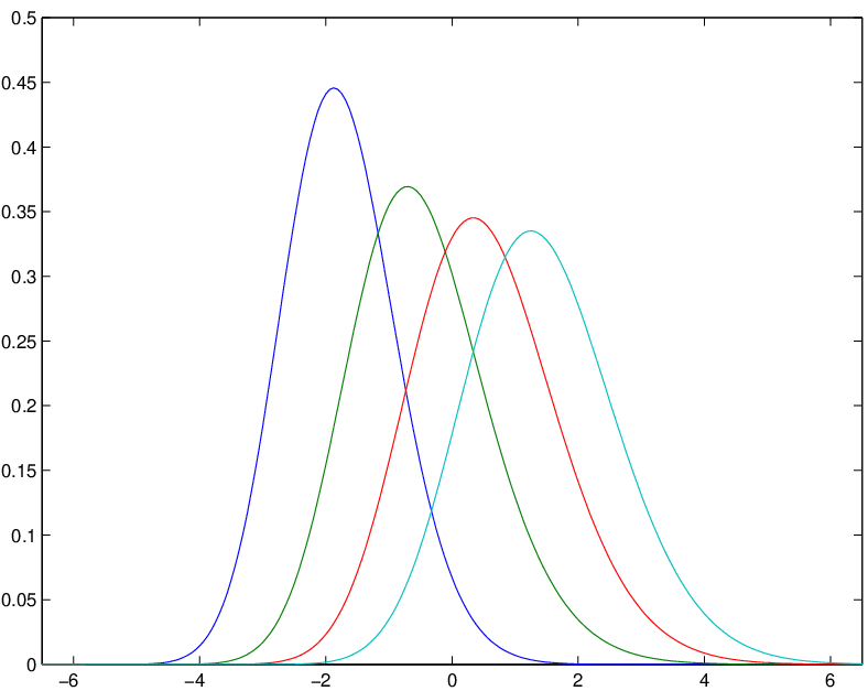
Note that the function moves to the right as the index $k$ increases. The numerical means and the standard deviations of $F_{k}(x)$ are the following:

mean standard deviation $F_{0}$ -1.771… 0.90… $F_{1}$ -0.494… 1.11… $F_{2}$ 0.543… 1.18… $F_{3}$ 1.445… 1.21…

1.1.5 $F_{k}$ are distribution functions

The Painlev’e formula obtained above can be used to prove that $F_{k}(x;w_{1},\dots,w_{k})$ is indeed a distribution function.

Corollary 1.6.

The function $F_{k}(x;w_{1},\dots,w_{k})$ is a distribution for real $w_{1},\dots,w_{k}$ .

Proof.

In [1], the function $F_{k}(x;w_{1},\dots,w_{k})$ are shown to be continuous, non-decreasing and converges to $1$ as $x\to+\infty$ (see the paragraph after (25)). We need to show that $F_{k}(x;w_{1},\dots,w_{k})\to 0$ as $x\to-\infty$ . From (1.25), all entries of the determinant in both (1.16) and (1.39) are in absolute value less than or equal to $Ce^{-c|x|^{3/2}}$ for some constants $C,c>0$ as $x\to-\infty$ . Also $F_{0}(x)\leq Ce^{-c|x|^{3}}$ for some other constants $C,c>0$ (see e.g. (2.13) of [4]). Hence $F_{k}(x;w_{1},\dots,w_{k})=O(e^{-c|x|^{3}})$ for some constant $c>0$ as $x\to-\infty$ . ∎

1.2 Outline of the proof and orthogonal polynomials on the unit circle

Theorem 1.1 is obtained by applying a sequence of row and column operations to the determinant (1.11). This part is the main bulk of the paper and the proof is given in Section 3.

The proof of Theorem 1.2 is indirect. We use a representation of orthogonal polynomials on the unit circle in terms of an operator on a discrete set. Since such a representation may be interesting in itself, we state it here. This formula follows from a general identity (see (4.1) below) between Toeplitz determinants and Fredholm determinants on integer lattice obtained by Geronimo and Case [14], and also independently by Borodin and Okounkov [7] (see also [6, 9] for shorter proofs).

Set $\mathbb{N}_{0}:=\mathbb{N}\cup\{0\}$ . Let $\phi(z)$ be a function which is positive on the unit circle. For simplicity of argument, we assume that $\phi(z)$ is analytic in neighborhood of the unit circle. Let $\phi=\phi_{+}\phi_{-}$ be a Wiener-Hopf factorization of $\phi$ where $\phi_{+}$ extends to a non-vanishing analytic function interior of the circle and $\phi_{-}$ extends to a non-vanishing analytic function exterior of the circle. Set

\psi(z):=\frac{\phi_{+}(z)}{\phi_{-}(z)}.

(1.41)

For a function $f(z)$ on the unit circle, $f_{k}$ denotes its $k^{th}$ Fourier coefficient:

f_{k}:=\int_{|z|=1}z^{-k}f(z)\frac{dz}{2\pi iz}.

(1.42)

Proposition 1.7.

Let $\pi_{n}(z)$ be the monic orthogonal polynomial on the unit circle with respect to the measure $\phi(z)\frac{dz}{2\pi iz}$ , and let $\pi_{n}^{*}(z)=z^{n}\overline{\pi}_{n}(\frac{1}{z})$ be its $*$ -transform. For $\phi$ satisfying above conditions,

\pi_{n}^{*}(z)=e^{-\sum_{k=1}^{\infty}(\log\phi)_{k}z^{k}}\biggl\{1-<\frac{1}{1-P_{n}ABP_{n}}P_{n}Q,P_{n}R>_{\ell^{2}(\mathbb{N}_{0})}\biggr\},\qquad|z|<1,

(1.43)

where $<,>_{\ell^{2}(\mathbb{N}_{0})}$ is the real inner product on $\ell^{2}(\mathbb{N}_{0})$ , $P_{n}$ is the projection on the set $\{n,n+1,n+2,\dots\}$ , the operators $A,B:\ell^{2}(\mathbb{N}_{0})\to\ell^{2}(\mathbb{N}_{0})$ are defined by the kernels

A(j,m)=(\psi^{-1})_{j+m+1},\qquad B(m,k)=\psi_{-m-k-1}

(1.44)

and the functions $Q,R\in\ell^{2}(\mathbb{N}_{0})$ are given by

Q(j)=(\psi^{-1})_{j+1},\qquad R(k)=\biggl(\frac{z}{\cdot-z}\psi(\cdot)\biggr)_{-k-1}=\int_{|b|=1}b^{k+1}\frac{z}{b-z}\psi(b)\frac{db}{2\pi ib}.

(1.45)

On the other hand,

\pi_{n}(z)=z^{n}e^{-\sum_{k=1}^{\infty}(\log\phi)_{-k}z^{-k}}\biggl\{1-<\frac{1}{1-P_{n}ABP_{n}}P_{n}U,P_{n}V>_{\ell^{2}(\mathbb{N}_{0})}\biggr\},\qquad|z|>1,

(1.46)

where

U(j)=\biggl(\frac{\cdot}{z-\cdot}\psi^{-1}(\cdot)\biggr)_{j+1}=\int_{|a|=1}a^{-j-1}\frac{a}{z-a}\frac{1}{\psi(a)}\frac{da}{2\pi ia},\qquad V(k)=\psi_{-k-1},

(1.47)

Remark.

(i) As $\pi_{n}^{*}(z)$ is an entire function, the formula (1.43) also holds for a region of $|z|\geq 1$ to which the right-hand-side of (1.43) is analytically continued. (ii) The conditions for $\phi$ above can be weakened, but we do not discuss such an issue in this paper. (iii) Recall that Wiener-Hopf factorizations of $\phi$ are different by a factor of a multiplicative constant. However, since $A$ and $B$ have both factors $\psi^{-1}$ and $\psi$ , respectively, the operator $AB$ is unaffected by a different choice of $\phi_{+}$ and $\phi_{-}$ . The inner products in (1.43) and (1.46) also remain the same even if $\psi$ is multiplied by a constant. Therefore, (1.43) and (1.46) does not depend on the choice of a Wiener-Hopf factorization of $\phi$ .

Remark.

After this paper was completed, it turned out during a conversation with Andrei Martínez-Finkelstein that (1.46) appeared in [22] in a very different form. In the first formula of the equation (32) of [22], the authors found a series expansion for $\pi(z)$ . However one can check that the series is precisely what one would obtain once the Neuman series of the operator $P_{n}ABP_{n}$ is taken in (1.46). The proof of [22] is based on a Riemann-Hilbert method. By turning the argument backward, it is also possible to prove the identity of Geromino-Case and Borodin-Okounkov using a Riemann-Hilbert method. This will appear in a future work.

We regard (1.43) as an identity. We take a special choice of $\phi$ and then take a limit of both sides of the identity (1.43). A steepest-descent analysis shows that the right-hand-side converges to the formula (1.15). On the other hand, a Riemann-Hilbert asymptotic analysis to the left-hand-side yields the Painlevé formula (1.20). Hence the identity (1.20) follows from the identity between the orthogonal polynomials and their operator representation.

This paper is organized as follows. In Section 2, we present the statistical and probabilistic models in which the distributions $F_{k}(x;w_{1},\dots,w_{k})$ appear. The proof of Theorem 1.1 is given in Section 3. Section 4 proves Proposition 1.7 and Section 5 proves Theorem 1.2.

Acknowledgments. The authors would like to thank P. Deift, A. Its, A. Martínez-Finkelshtein, B. Simon and H. Widom for useful conversations and communications. This work was supported in part by NSF Grant #DMS-0350729 and the AMS Centennial Fellowship.

2 Models

We discuss several statistics and probability models in which $F_{k}$ ’s appear.

2.1 Non-null complex sample covariance matrices

Let $M\geq N\geq 1$ be integers. Let $\vec{y}_{1},\dots,\vec{y}_{M}$ be independent complex Gaussian $N\times 1$ column vectors with mean $\vec{\mu}$ and population covariance $\Sigma$ : the density of $\vec{y}_{1}$ is

p(\vec{y}_{1})=\frac{1}{(2\pi)^{N/2}(\det\Sigma)^{1/2}}e^{-\frac{1}{2}(\vec{y}_{1}-\vec{\mu})^{*}\Sigma^{-1}(\vec{y}_{1}-\vec{\mu})}

(2.1)

where $*$ denotes the complex transpose. Denote by $\bar{Y}$ the sample mean $\bar{Y}:=\frac{1}{M}(\vec{y}_{1}+\dots+\vec{y}_{M})$ and by $X=[\vec{y}_{1}-\bar{Y},\dots,\vec{y}_{M}-\bar{Y}]$ the (centered) $M\times N$ sample matrix. Define the sample covariance matrix by

S=\frac{1}{M}XX^{*}.

(2.2)

When the covariance matrix $\Sigma$ is the identity matrix, the distribution of the eigenvalues of $S$ is sometimes called the Laguerre unitary ensemble and is well-studied in the random matrix theory (see e.g. [12]). In particular, as $M,N\to\infty$ while $M/N=\gamma^{2}$ is in a compact subset of $[1,\infty)$ , the largest eigenvalue $\lambda_{\max}$ satisfies the limit law (see e.g. [13, 19])

\Prob\biggl(\bigl(\lambda_{\max}-(1+\gamma^{-1})^{2})\bigr)\cdot\frac{\gamma}{(1+\gamma)^{4/3}}M^{2/3}\leq x\biggr)\to F_{0}(x),

(2.3)

where $F_{0}(x)$ is the Tracy-Widom distribution (1.3).

Johnstone [21] proposed the study of the so-called the ‘spiked population model’ where the covariance matrix $\Sigma$ is a finite rank perturbation of the identity matrix. For possible applications of the spiked population model in statistics, finance and telecommunications, see the references in [21] and [1]. For spiked population models, it is interesting to determine the effect of non-unit eigenvalues of the covariance matrix on the largest eigenvalue of the sample covariance matrix. For complex Gaussian samples, [1] determined the critical value of the non-unit covariance eigenvalue. When some of the non-unit eigenvalues of the covariance matrix are above the critical value, $\lambda_{\max}$ behaves differently from (2.3). The function $F_{k}(x)$ is the limiting distribution of the $\lambda_{\max}$ when the largest eigenvalue of the covariance matrix is of multiplicity $k$ and is equal to the critical value.

Let $\ell_{1}\geq\dots\geq\ell_{r}>0$ be the non-unit eigenvalues of $\Sigma$ where $r$ is independent of $M$ and $N$ .

Theorem 2.1 (Theorem 1.1 of [1]).

As $M,N\to\infty$ such that $M/N=\gamma^{2}$ lies in a compact subset of $[1,\infty)$ , the following holds.

(a)

When

\ell_{1}=\dots=\ell_{k}=1+\gamma^{-1}

(2.4)

for some $0\leq k\leq r$ , and $\ell_{k+1},\dots,\ell_{r}$ are in a compact subset of $(0,1+\gamma^{-1})$ ,

\Prob\biggl(\bigl(\lambda_{\max}-(1+\gamma^{-1})^{2})\bigr)\cdot\frac{\gamma}{(1+\gamma)^{4/3}}M^{2/3}\leq x\biggr)\to F_{k}(x)

(2.5)

where $F_{k}(x)$ is defined in (1.13).

(b)

When

\ell_{1}=\dots=\ell_{k}

are in a compact subset of

(1+\gamma^{-1},\infty)

(2.6)

for some $1\leq k\leq r$ , and $\ell_{k+1},\dots,\ell_{r}$ are in a compact subset of $(0,\ell_{1})$ ,

\Prob\biggl(\bigl(\lambda_{\max}-(\ell_{1}+\frac{\ell_{1}\gamma^{-2}}{\ell_{1}-1})\bigr)\cdot\sqrt{M}\sqrt{\ell_{1}^{2}-\frac{\ell_{1}^{2}\gamma^{-2}}{(\ell_{1}-1)^{2}}}\leq x\biggr)\to G_{k}(x)

(2.7)

where $G_{k}(x)$ is the distribution of the largest eigenvalue of $k\times k$ Gaussian unitary ensemble.

More detailed nature of the phase transition around the critical value $1+\gamma^{-1}$ was also studied in the same paper.

Theorem 2.2 (Theorem 1.2 of [1]).

For some $1\leq k\leq r$ , set

\ell_{j}=1+\gamma^{-1}-\frac{(1+\gamma)^{3/2}w_{j}}{\gamma M^{1/3}},\qquad j=1,2,\dots,k.

(2.8)

When $w_{1},\dots,w_{k}$ are in a compact subset of $\mathbb{R}$ and $\ell_{k+1},\dots,\ell_{r}$ are in a compact subset of $(0,1+\gamma^{-1})$ , as $M,N\to\infty$ while $M/N=\gamma^{2}$ is in a compact subset of $[1,\infty)$ ,

\Prob\biggl(\bigl(\lambda_{\max}-(1+\gamma^{-1})^{2})\bigr)\cdot\frac{\gamma}{(1+\gamma)^{4/3}}M^{2/3}\leq x\biggr)\to F_{k}(x;w_{1},\dots,w_{k})

(2.9)

where $F_{k}(x;w_{1},\dots,w_{k})$ is defined in (1.11).

It is transparent from this theorem that $F_{k}(x;w_{1},\dots,w_{k})$ should be symmetric in $w_{1},\dots,w_{k}$ since re-labelling the eigenvalues does not change the limit law. Further work on the eigenvalues of the spiked model can be found in [24, 5].

2.2 Last passage percolation and queues in tandem

Suppose that to each lattice points $(i,j)\in\mathbb{Z}^{2}$ , an independent random variable $X(i,j)$ is associated. Let $(1,1)\nearrow(N,M)$ denote the set of ‘up/right paths’ $\pi=\{(i_{k},j_{k})\}_{k=1}^{N+M-1}$ where $(i_{k+1},j_{k+1})-(i_{k},j_{k})$ is either $(1,0)$ or $(0,1)$ , and $(i_{1},j_{1})=(1,1)$ and $(i_{N+M-1},j_{N+M-1})=(N,M)$ . Note that the cardinality of $(1,1)\nearrow(N,M)$ is $\binom{N+M-2}{N-1}$ . Set

L(N,M):=\max_{\pi\in(1,1)\nearrow(N,M)}\sum_{(i,j)\in\pi}X(i,j).

(2.10)

By interpreting $X(i,j)$ as the (random) time spent to pass the site $(i,j)$ , $L(N,M)$ is the last passage time to travel from $(1,1)$ to $(N,M)$ along an admissible up/right path.

Recall that the exponential random variable of mean $m$ has the density function $\frac{1}{m}e^{-x/m}$ , $x\geq 0$ . It is known that (see e.g. Proposition 6.1 of [1]; we here scale $X(i,j)$ of [1] by $M$ ) when $X(i,j)$ is an exponential random variable of mean $\ell_{i}$ (independent of $j$ ), $\frac{L(N,M)}{M}$ has the same distribution as the largest sample eigenvalue $\lambda_{\max}$ of complex Gaussian samples when the eigenvalues of the population covariance matrix $\Sigma$ are $\ell_{1},\dots,\ell_{N}$ . Therefore for the last passage percolation model which have the identically distributed passage time for all but finitely many columns, Theorems 2.1 and Theorem 2.2 also hold with $\lambda_{\max}$ replaced by $\frac{L(N,M)}{M}$ . In particular, Theorem 2.1 shows that as long as the site passage time on the distinguished columns have mean less than $1+\gamma^{-1}$ , the last passage time has the same limit behavior as the case when all the sites are identically distributed.

2.3 Queues in tandem

Suppose that there are $N$ servers and $M$ customers. Initially all the customers are at the first server in a queue. Once a customer is served at a server, then (s)he moves to the queue of the next server and waits for his/her turn. The service time for the $j$ th customer at the $i$ th server is assumed to be a random variable $X(i,j)$ and let $D(N,M)$ be the departure time of all the customers from all the queues. It is well-known that $D(N,M)$ has the same distribution as $L(N,M)$ of the last passage percolation model (see e.g. [15]).

In the queueing theory context, Theorem 2.1 determines the effect of a few slow servers to the total departure time. Suppose that $X(i,j)$ is an exponential random variable of mean $1$ for $i=r+1,\dots,N$ (independent of $i$ ) and of mean $\ell_{i}$ for $i=1,\dots,r$ . In other words, the service times at the first $r$ servers are distributed differently from those at the rest of the servers. When all of $\ell_{i}$ are not so large, the departure time has the same limiting law as when all the service times are identically distributed, but the whole process slows down when some of the servers are sufficiently slow. Theorem 2.1 shows that the critical value is $\ell_{i}=1+\gamma^{-1}$ . Note that due to a symmetry between servers and customers, the theorem also applies to slow customers.

2.4 Totally asymmetric simple exclusion process

The last passage percolation can also be interpreted as an interacting particle systems (see e.g. [25, 19]). We will consider the totally asymmetric simple exclusion process. Let $x_{j}(t)\in\mathbb{Z}$ , $x_{j}(t)$ , $j=1,2,\dots$ , $t\in[0,\infty)$ , denote the location of the $j$ th particle at time $t$ . A particle can jump only to its right neighboring site after random time if the site is not occupied. Let $X(i,j)$ be independent random variables which represent the $i$ th jumping time of the $j$ th particle. We take the initial condition as $x_{j}(0)=1-j$ , $j=1,2,\dots$ . Then $X(i,j)$ is the time it takes for the $j$ th particle $x_{j}$ to jump from the site $i-j$ to $i-j+1$ .

Let $T(i,j)$ be the time it takes for the $j$ th particle to arrive at the location $i-j+1$ . Equivalently, $T(i,j)$ is the time it takes for the $j$ th particle to perform the first $i$ jumps. Note that in order for the $j$ th particle to jump from the site $i-j$ to $i-j+1$ , the $(j-1)$ th particle should be to the right of the site $i-j+1$ . Hence we find that

T(i,j)=\max\{T(i-1,j),T(i,j-1)\}+X(i,j),\qquad i,j\geq 1,

(2.11)

where $T(0,j)=T(i,0)=0$ , $i,j\geq 1$ , by definition. A simple geometric consideration shows that last passage time $L(i,j)$ satisfies exactly the same recurrence relation. Therefore $T(i,j)$ is same as the last passage time in the sense of distribution.

Let $\#(m,t)$ denote the number of particles to the right of the site $m$ at time $t$ . The flux $F(m,t)$ , the number of particles that have jumped cross the interval $(m,m+1)$ up to time $t$ , is then $F(m,t)=\#(m,t)$ for $m>0$ , and $F(m,t)=\#(m,t)+m$ for $m\leq 0$ . The event that $\#(m,t)\geq M$ is same as the event that the $M$ th particle is to the right of the site $m$ at time $t$ . This is again equal to the event that $T(m+M,M)\leq t$ , and hence we find that $\mathbb{P}(\#(m,t)\geq M)=\mathbb{P}(T(m+M,M)\leq t)=\mathbb{P}(L(m+M,M)\leq t)$ . Therefore, Theorem 2.1 and Theorem 2.2 again apply to $\#([ut],t)$ , and hence to $F([ut],t)$ . We state the results for $\#([ut],t)$ here.

Traffic of slow start from stop

Suppose that $X(i,j)$ is an independent exponential random variable of mean $\ell_{i}$ for $i=1,\dots,r$ and of mean $1$ for $i>r$ (independent of $j$ ). In other words, each particle jumps at rate $\frac{1}{\ell_{i}}$ for its first $r$ jumps and then jumps at rate $1$ afterwards. When $\ell_{1}\geq\dots\geq\ell_{r}$ , one can view it as a toy model for the following traffic situation: (infinite) cars in one lane, which were fully stopped at the red signal, speed up at the green signal until they finally reach the steady speed (after $r$ ‘jumps’). Set $\ell=\max\{\ell_{1},\dots,\ell_{r}\}$ and let $k\geq 1$ be the number of $\ell_{i}$ ’s equal to $\ell$ . By re-interpreting Theorem 2.1, a tedious but straightforward calculation shows the following results for $-1<u\leq 0$ :

\lim_{t\to\infty}\mathbb{P}\biggl(\#([ut],t)\geq\frac{1}{4}(1-u)^{2}t+x\biggl(\frac{1-u^{2}}{4}\biggr)^{2/3}t^{1/3}\biggr)=\begin{cases}F_{0}(-x),\qquad&u\in\bigl(1-\frac{2}{\ell},0]\cap(-1,0]\\ F_{k}(-x),\qquad&u=1-\frac{2}{\ell}\in(-1,0],\end{cases}

(2.12)

and for $u\in\bigl(\frac{1}{-\ell},1-\frac{2}{\ell}\bigr)\cap(-1,0]$ ,

\lim_{t\to\infty}\mathbb{P}\biggl(\#([ut],t)\geq\frac{\ell-1-\ell u}{\ell^{2}}t+x\frac{(\ell-1)^{3/2}(\ell-1-\ell u)}{\ell^{9/2}(\ell-2-\ell u)^{1/2}}t^{1/2}\biggr)=G_{k}(-x).

(2.13)

This shows that fast jumps do not affect the flux but slow jumps may change the flux. When $r=0$ (all cars jumping at the same rate), (2.12) was first obtained in [19] for $0\leq u<1$ .

Traffic with a few slow cars

The exclusion process of the particles yields a dual process of the holes. As the particles jump to the right, the holes, the unoccupied sites, jump to the left. The leftmost hole jumps at rate $\frac{1}{\ell_{1}}$ since each particle jump at that rate at its first jump. Likewise, the second leftmost hole jumps at rate $\frac{1}{\ell_{2}}$ and so on. Hence this model can be thought of traffic model where there are a few cars of distinguished jump rates. Initially the holes are at the sites $\{1,2,3,\dots\}$ . As the number of holes $\mathcal{H}(m,t)$ on the left of the site $m+1$ at time $t$ satisfies $\mathcal{H}(m,t)=\#(m,t)+m$ , (2.12) and (2.13) imply the following results for $-1<u\leq 0$ :

\lim_{t\to\infty}\mathbb{P}\biggl(\mathcal{H}([ut],t)\geq\frac{1}{4}(1+u)^{2}t+x\biggl(\frac{1-u^{2}}{4}\biggr)^{2/3}t^{1/3}\biggr)=\begin{cases}F_{0}(-x),\qquad&u\in\bigl(1-\frac{2}{\ell},0]\cap(-1,0]\\ F_{k}(-x),\qquad&u=1-\frac{2}{\ell}\in(-1,0],\end{cases}

(2.14)

and for $u\in\bigl(\frac{1}{-\ell},1-\frac{2}{\ell}\bigr)\cap(-1,0]$ ,

\lim_{t\to\infty}\mathbb{P}\biggl(\mathcal{H}([ut],t)\geq\frac{\ell-1-\ell u+\ell^{2}u}{\ell^{2}}t+x\frac{(\ell-1)^{3/2}(\ell-1-\ell u)}{\ell^{9/2}(\ell-2-\ell u)^{1/2}}t^{1/2}\biggr)=G_{k}(-x).

(2.15)

The full case of $-1<u<1$ and also correlation functions of various locations for both of the above traffic models will be discussed in a forthcoming paper.

3 Proof of Theorem 1.1

We prove Theorem 1.1 in this section.

Since both sides of (1.16) are analytic in each $w_{j}$ , the case when some of $w_{j}$ ’s coincide follows from analytic continuation of the case when all $w_{j}$ ’s are distinct. Hence we assume in this section that all $w_{j}$ ’s are distinct. We need to prove that

\begin{split}&\det\biggl(\delta_{mn}-<\frac{1}{1-\mathbf{A}_{x}}s^{(m)}(w_{1},\dots,w_{m}),t^{(n)}(w_{1},\dots,w_{n-1})>_{(x,\infty)}\biggr)_{1\leq m,n\leq k}\\ &=\frac{1}{\displaystyle\prod_{1\leq m<n\leq k}(w_{n}-w_{m})}\det\begin{pmatrix}(w_{m}+D_{x})^{n-1}f(x,w_{m})\end{pmatrix}_{1\leq m,n\leq k}.\end{split}

(3.1)

Notational Remark.

In the below, we sometimes have a product of empty indices. For instance when $n=1$ , the product $\displaystyle\prod_{a=1}^{n-1}(w_{a}-w_{i})$ in (3.11) has no indices. In such cases, we interpret the product as $1$ .

Let $\mathbb{A}_{x}:L^{2}((0,\infty))\to L^{2}((0,\infty))$ be the operator with kernel

\mathbb{A}_{x}(u,v)=\mathbf{A}(u+x,v+x).

(3.2)

Set

S_{m}(u)=s^{(m)}(u+x)=s^{(m)}(u+x;w_{1},\dots,w_{m})

(3.3)

and set

T_{m}(v)=t^{(m)}(v+x)=t^{(m)}(v+x;w_{1},\dots,w_{m-1}).

(3.4)

Then

\biggl(\frac{1}{1-\mathbf{A}_{x}}s^{(m)}\biggr)(u+x)=\biggl(\frac{1}{1-\mathbb{A}_{x}}S_{m}\biggr)(u)

(3.5)

and the matrix on the left-hand-side of (3.1) is

\bigl(\delta_{ij}-<\frac{1}{1-\mathbb{A}_{x}}S_{i},T_{j}>\bigr)_{1\leq i,j\leq k}

(3.6)

where $<,>=<,>_{(0,\infty)}$ is the real inner product in $L^{2}((0,\infty))$ .

Since

\prod_{j=1}^{m}\frac{1}{w_{j}+ia}=\sum_{j=1}^{m}\frac{1}{w_{j}+ia}\displaystyle\prod_{\begin{subarray}{c}\ell=1\\ \ell\neq j\end{subarray}}^{m}\frac{1}{w_{\ell}-w_{j}},

(3.7)

we find

\biggl(\frac{1}{1-\mathbb{A}_{x}}S_{m}\biggr)(u)=\sum_{j=1}^{m}\biggl[\displaystyle\prod_{\begin{subarray}{c}\ell=1\\ \ell\neq j\end{subarray}}^{m}\frac{1}{w_{\ell}-w_{j}}\biggr]E_{w_{j}}(u).

(3.8)

where

E_{w}(u)=E_{w}(u;x):=\biggl(\frac{1}{1-\mathbb{A}_{x}}\widetilde{C}_{w}\biggr)(u),\qquad\widetilde{C}_{w}(u):=C_{w}(u+x)

(3.9)

(recall (1.14) for the definition of $C_{w}$ ). For later use, we note that $f(x,w)$ defined in (1.15) satisfies that

f(x,w)=1-<E_{w},T_{1}>.

(3.10)

Now we invert the relation (3.8). For $1\leq m\leq k$ , (3.8) is a system of $k$ linear equations for $E_{w_{j}}$ , $1\leq j\leq k$ .

Lemma 3.1.

The equation (3.8) for $E_{w_{j}}$ has the solution given by

E_{w_{j}}(u)=\sum_{n=1}^{j}\biggl[\prod_{a=1}^{n-1}(w_{a}-w_{j})\biggr]\biggl(\frac{1}{1-\mathbb{A}_{x}}S_{n}\biggr)(u).

(3.11)

Proof.

Consider the function

F(z):=-\prod_{\ell=n}^{m}\frac{1}{w_{\ell}-z}.

(3.12)

Integrating over a circle of radius $R$ , and then taking $R\to\infty$ , we find that the sum of residues of $F$ is equal to $0$ when $m-n\geq 1$ and is equal to $1$ when $m=n$ . On the other hand, by directly computation, the residue of $F$ at $z=w_{j}$ is

\prod_{\begin{subarray}{c}\ell=n\\ \ell\neq j\end{subarray}}^{m}\frac{1}{w_{\ell}-w_{j}}.

(3.13)

Hence we obtain the identity

\sum_{j=n}^{m}\prod_{\begin{subarray}{c}\ell=n\\ \ell\neq j\end{subarray}}^{m}\frac{1}{w_{\ell}-w_{j}}=\delta_{mn},\qquad m\geq n.

(3.14)

Now as all $w_{i}$ ’s are distinct, the determinant of the matrix for the linear equation (3.8) is $\prod_{1\leq\ell<m\leq k}(w_{\ell}-w_{m})^{-1}$ , which is non-zero. Hence there is a unique solution $E_{w_{j}}$ for (3.8). We should check that (3.11) solves (3.8). But this follows by inserting (3.11) into the right-hand-side of (3.8), changing the order of summations, and then using (3.14). ∎

From (3.11), we obtain for each $1\leq i,j\leq k$ ,

\sum_{n=1}^{i}\prod_{a=1}^{n-1}(w_{a}-w_{i})\cdot\bigl(\delta_{nj}-<\frac{1}{1-\mathbb{A}_{x}}S_{n},T_{j}>\bigr)=F_{ij}-<E_{w_{i}},T_{j}>

(3.15)

where

F_{ij}:=\prod_{a=1}^{j-1}(w_{a}-w_{i}).

(3.16)

Note that $F_{ij}=0$ when $i<j$ . Now we perform row operations of the matrix $\bigl(\delta_{ij}-<\frac{1}{1-\mathbb{A}_{x}}S_{i},T_{j}>\bigr)_{1\leq i,j\leq k}$ using (3.15) that replaces the $i$ th row by a linear combination of the first $i$ rows to find that

\begin{split}\det\bigl(\delta_{ij}-<\frac{1}{1-\mathbb{A}_{x}}S_{i},T_{j}>\bigr)_{k\times k}&=\prod_{i=1}^{k}\prod_{a=1}^{i-1}\frac{1}{w_{a}-w_{i}}\cdot\det\bigl(F_{ij}-<E_{w_{i}},T_{j}>\bigr)_{k\times k}\\ &=\frac{1}{\displaystyle\prod_{1\leq i<j\leq k}(w_{i}-w_{j})}\cdot\det\bigl(F_{ij}-<E_{w_{i}},T_{j}>\bigr)_{k\times k}.\end{split}

(3.17)

Note that the when $j=1$ , $F_{ij}=1$ , (see the Notational Remark above) and hence the first column of the matrix $\bigl(F_{ij}-<E_{w_{i}},T_{j}>\bigr)_{k\times k}$ consists of the functions (see (3.10))

1-<E_{w_{i}},T_{1}>=f(x,w_{i}).

(3.18)

For example, when $k=3$ , the determinant on the right-hand-side of (3.17) is

\det\begin{pmatrix}f(x,w_{1})&-<E_{w_{1}},T_{2}>&-<E_{w_{1}},T_{3}>\\ f(x,w_{2})&(w_{1}-w_{2})-<E_{w_{2}},T_{2}>&-<E_{w_{2}},T_{3}>\\ f(x,w_{3})&(w_{1}-w_{3})-<E_{w_{3}},T_{2}>&(w_{1}-w_{3})(w_{2}-w_{3})-<E_{w_{3}},T_{3}>\end{pmatrix}.

(3.19)

From the definition (3.4) of $T_{j}$ and the definition (1.10) of $t_{j}$ , we have

T_{j}=w_{j-1}T_{j-1}-D_{x}T_{j-1},\qquad j\geq 2.

(3.20)

Set $M^{(0)}$ be the matrix

M^{(0)}:=\bigl(F_{ij}-<E_{w_{i}},T_{j}>\bigr)_{1\leq i,j\leq k}.

(3.21)

Let $M^{(1)}$ be the matrix defined by

M^{(1)}:=M^{(0)}\begin{pmatrix}1&-w_{1}&0\\ 0&1&-w_{2}&0\\ &0&1&-w_{3}&0\\ &&&\ddots&\ddots&\\ &&&&\ddots&\ddots&\\ &&&&0&1&-w_{k-1}\\ &&&&&0&1\end{pmatrix},

(3.22)

whose determinant is same as the determinant of $M^{(0)}$ . Using the relation (3.20), the entries of $M^{(1)}=\bigl(M^{(1)}_{ij}\bigr)_{1\leq i,j\leq k}$ are given by

M^{(1)}_{ij}=\begin{cases}f(x,w_{i}),\qquad&j=1\\ -\bigl(F_{ij}^{(1)}-<E_{w_{i}},D_{x}T_{j-1}>),\qquad&2\leq j\leq k,\end{cases}

(3.23)

where

F_{ij}^{(1)}:=w_{j-1}F_{i,j-1}-F_{ij}.

(3.24)

Now define a new matrix $M^{(2)}=\bigl(M^{(2)}_{ij}\bigr)_{1\leq i,j\leq k}$ by

M^{(2)}:=M^{(1)}\begin{pmatrix}1&0&0\\ 0&1&-w_{1}&0\\ &0&1&-w_{2}&0\\ &&&\ddots&\ddots&\\ &&&&\ddots&\ddots&\\ &&&&0&1&-w_{k-2}\\ &&&&&0&1\end{pmatrix}.

(3.25)

Using the relation

D_{x}T_{j-1}=w_{j-2}D_{x}T_{j-2}-D_{x}^{2}T_{j-2}

(3.26)

that follows from (3.20) for $3\leq j\leq k$ , we find that

M^{(2)}_{ij}=\begin{cases}f(x,w_{i}),\qquad&j=1\\ -\bigl(F_{i2}^{(1)}-<E_{w_{i}},D_{x}T_{1}>),\qquad&j=2\\ F_{ij}^{(2)}-<E_{w_{i}},D_{x}^{2}T_{j-2}>,\qquad&3\leq j\leq k,\end{cases}

(3.27)

where

F_{ij}^{(2)}:=w_{j-2}F_{i,j-1}^{(1)}-F_{ij}^{(1)}.

(3.28)

Continuing in a similar way, we eventually define

\begin{split}M^{(k-1)}:=M^{(0)}&\begin{pmatrix}1&-w_{1}&0\\ 0&1&-w_{2}&0\\ &0&1&-w_{3}&0\\ &&&\ddots&\ddots&\\ &&&&\ddots&\ddots&\\ &&&&0&1&-w_{k-1}\\ &&&&&0&1\end{pmatrix}\times\begin{pmatrix}1&0&0\\ 0&1&-w_{1}&0\\ &0&1&-w_{2}&0\\ &&&\ddots&\ddots&\\ &&&&\ddots&\ddots&\\ &&&&0&1&-w_{k-2}\\ &&&&&0&1\end{pmatrix}\\ &\times\cdots\times\begin{pmatrix}1&0&0\\ 0&1&0&0\\ &0&1&0&0\\ &&&\ddots&\ddots&\\ &&&&\ddots&\ddots&\\ &&&&0&1&-w_{1}\\ &&&&&0&1\end{pmatrix}.\end{split}

(3.29)

Using the fact that for all $\ell\geq 1$ , $j\geq 2$ ,

D_{x}^{\ell}T_{j}=w_{j-1}D_{x}^{\ell}T_{j-1}-D_{x}^{\ell+1}T_{j-1},

(3.30)

we find that

M^{(k-1)}_{ij}=(-1)^{j-1}\bigl(F_{ij}^{(j-1)}-<E_{w_{i}},D_{x}^{j-1}T_{1}>\bigr),\qquad 1\leq i,j\leq k,

(3.31)

where for each $1\leq i\leq k$ , $F_{ij}^{(\ell)}$ is inductively defined by the relation

F_{ij}^{(\ell)}:=w_{j-\ell}F_{i,j-1}^{(\ell-1)}-F_{ij}^{(\ell-1)},\qquad 1\leq\ell<j\leq k

(3.32)

and (see (3.16))

F_{ij}^{(0)}:=F_{ij}=\prod_{a=1}^{j-1}(w_{a}-w_{i}),\qquad 1\leq j\leq k.

(3.33)

Recall that $F_{i1}=1$ , and hence $M^{(k-1)}_{i1}=1-<E_{w_{i}},T_{1}>=f(x,w_{i})$ .

Lemma 3.2.

The solution $F_{ij}^{(\ell)}$ to the recurrence relation (3.32) and (3.33) is

F_{ij}^{(\ell)}=w_{i}^{\ell}\prod_{a=1}^{j-\ell-1}(w_{a}-w_{i}),\qquad 1\leq\ell<j\leq k.

(3.34)

Proof.

This follows easily from an induction in $\ell$ . Here, as mentioned in the Notational Remark above, when $j=\ell+1$ , we understand that the product $\prod_{a=1}^{0}(w_{a}-w_{i})=1$ . ∎

Therefore $F^{(j-1)}_{ij}=w_{i}^{j-1}$ , and as $\det(M^{(0)})=\det(M^{(k-1)})$ , we find from (3.17), (3.21) and (3.31) that

\begin{split}\det\bigl(\delta_{ij}-<\frac{1}{1-\mathbb{A}_{x}}S_{i},T_{j}>\bigr)_{1\leq i,j\leq k}=\frac{(-1)^{[k/2]}}{\displaystyle\prod_{1\leq i<j\leq k}(w_{i}-w_{j})}\det\bigl(M\bigr),\end{split}

(3.35)

where $[k/2]$ denotes the largest integer smaller than or equal to $k/2$ , and the $k\times k$ matrix $M=\bigl(M_{ij}\bigr)_{1\leq i,j\leq k}$ is given by

M_{ij}=w_{i}^{j-1}-<E_{w_{i}},D_{x}^{j-1}T_{1}>.

(3.36)

As $\prod_{1\leq m<n\leq k}(-1)=(-1)^{[k/2]}$ , this is equal to

\begin{split}\det\bigl(\delta_{ij}-<\frac{1}{1-\mathbb{A}_{x}}S_{i},T_{j}>\bigr)_{1\leq i,j\leq k}=\frac{1}{\displaystyle\prod_{1\leq i<j\leq k}(w_{j}-w_{i})}\det\bigl(M\bigr),\end{split}

(3.37)

Now we will show that $\det(M)$ is equal to the determinant on the right-hand-side of (3.1). For this purpose, we use the following result.

Lemma 3.3.

For $\ell\geq 0$ , there are smooth functions $F_{\ell,a}(x)$ , $a=0,1,\dots,\ell-1$ , such that

(w+D_{x})^{\ell}f(x,w)=w^{\ell}-<E_{w},D_{x}^{\ell}T_{1}>-\sum_{a=0}^{\ell-1}F_{\ell,a}(x)(w+D_{x})^{a}f(x,w).

(3.38)

Proof.

From the definition of $E_{w}$ ,

D_{x}E_{w}=D_{x}\biggl(\frac{1}{1-\mathbb{A}_{x}}\widetilde{C}_{w}\biggr)=\frac{1}{1-\mathbb{A}_{x}}(D_{x}\mathbb{A}_{x})\frac{1}{1-\mathbb{A}_{x}}\widetilde{C}_{w}+\frac{1}{1-\mathbb{A}_{x}}D_{x}\widetilde{C}_{w}.

(3.39)

It is direct to check that $(D_{x}\mathbb{A}_{x})(u,v)=-\Ai(x+u)\Ai(x+v)$ . Hence $D_{x}\mathbb{A}_{x}=-T_{1}\otimes T_{1}$ . On the other hand, from the definition (1.14) of $C_{w}$ , $D_{x}\widetilde{C}_{w}=T_{1}-w\widetilde{C}_{w}$ . Hence we find

\begin{split}D_{x}E_{w}&=-\frac{1}{1-\mathbb{A}_{x}}T_{1}\otimes T_{1}\frac{1}{1-\mathbb{A}_{x}}\widetilde{C}_{w}+\frac{1}{1-\mathbb{A}_{x}}(T_{1}-w\widetilde{C}_{w})\\ &=-<T_{1},\frac{1}{1-\mathbb{A}_{x}}\widetilde{C}_{w}>\frac{1}{1-\mathbb{A}_{x}}T_{1}+\frac{1}{1-\mathbb{A}_{x}}T_{1}-w\frac{1}{1-\mathbb{A}_{x}}\widetilde{C}_{w},\end{split}

(3.40)

which implies that

(w+D_{w})E_{w}=f(x,w)\frac{1}{1-\mathbb{A}_{x}}T_{1}

(3.41)

Now we use an induction in $\ell$ to prove (3.38). When $\ell=0$ , by definition (1.15) of $f$ , (3.38) holds. Now suppose that (3.38) holds true for some $\ell\geq 0$ . Then using the general identities $(w+D_{x})<h,g>=<(w+D_{x})h,g>+<h,D_{x}g>$ and $(w+D_{x})\bigl(hg)=(D_{x}h)g+h\bigl((w+D_{x})g\bigr)$ ,

\begin{split}&(w+D_{x})^{\ell+1}f(x,w)\\ &\qquad=(w+D_{x})\bigl[(w+D_{x})^{\ell}f(x,w)\bigr]\\ &\qquad=(w+D_{x})\bigl[w^{\ell}-<E_{w},D_{x}^{\ell}T_{1}>-\sum_{a=0}^{\ell-1}F_{\ell,a}(x)(w+D_{x})^{a}f(x,w)\bigr]\\ &\qquad=w^{\ell+1}-<(w+D_{x})E_{w},D_{x}^{\ell}T_{1}>-<E_{w},D_{x}^{\ell+1}T_{1}>\\ &\qquad\quad-\sum_{a=0}^{\ell-1}\biggl\{\bigl(D_{x}F_{\ell,a}(x)\bigr)(w+D_{x})^{a}f(x,w)+F_{\ell,a}(x)(w+D_{x})^{a+1}f(x,w)\biggr\}\\ &\qquad=w^{\ell+1}-f(x,w)<\frac{1}{1-\mathbb{A}_{x}}T_{1},D_{x}^{\ell}T_{1}>-<E_{w},D_{x}^{\ell+1}T_{1}>\\ &\qquad\quad-\sum_{a=0}^{\ell-1}\biggl\{\bigl(D_{x}F_{\ell,a}(x)\bigr)(w+D_{x})^{a}f(x,w)+F_{\ell,a}(x)(w+D_{x})^{a+1}f(x,w)\biggr\},\end{split}

(3.42)

where (3.41) is applied in the last step. Therefore we find that (3.38) holds true for $\ell+1$ with the functions

F_{\ell+1,a}=\begin{cases}D_{x}F_{\ell,0}(x)+<\frac{1}{1-\mathbb{A}_{x}}T_{1},D_{x}^{\ell}T_{1}>,\qquad&a=0,\\ D_{x}F_{\ell,a}(x)+F_{\ell,a-1},\qquad&1\leq a\leq\ell-1,\\ F_{\ell,\ell-1},\qquad&a=\ell,\end{cases}

(3.43)

where $F_{0,0}:=0$ . ∎

By applying (3.38) repeatedly to $(w+D_{x})^{a}f(x;w)$ inside the summation on the right-hand-side of (3.38), for $\ell\geq 0$ , there are smooth functions $G_{\ell,a}$ , $a=0,1,\dots,\ell-1$ such that

w^{\ell}-<E_{w},D_{x}^{\ell}T_{1}>=(w+D_{x})^{\ell}f(x;w)+\sum_{a=0}^{\ell-1}G_{\ell,a}(x)\bigl(w^{a}-<E_{w},D_{x}^{a}T_{1}>\bigr).

(3.44)

Therefore for any $1\leq i\leq k$ ,

M_{ij}=w_{i}^{j-1}-<E_{w_{i}},D_{x}^{j-1}T_{1}>=(w_{i}+D_{x})^{j-1}f(x,w_{i})+\sum_{a=1}^{j-1}G_{j-1,a-1}(x)M_{ia}.

(3.45)

In other words, the $j$ th column vector in the matrix $M$ is equal to a linear combination of the first, second, …, $j-1$ th column vectors plus the vector $\bigl((w_{1}+D_{x})^{j-1}f(x,w_{1}),\cdots,(w_{k}+D_{x})^{j-1}f(x,w_{k})\bigr)^{T}$ . Hence by applying proper column operations, we find

\det(M)=\det\bigl((w_{i}+D_{x})^{j-1}f(x,w_{i})\bigr)_{1\leq i,j\leq k}.

(3.46)

This, together with (3.37), implies that the left-hand-side of (3.1) is equal to

\begin{split}\frac{1}{\displaystyle\prod_{1\leq m<n\leq k}(w_{n}-w_{m})}\det\begin{pmatrix}(w_{m}+D_{x})^{n-1}f(x,w_{m})\end{pmatrix}_{1\leq m,n\leq k}.\end{split}

(3.47)

This is the right-hand-side of (3.1) and Theorem 1.1 is proved.

4 Proof Proposition 1.7

Let $T_{n}(\varphi)=(\varphi_{i-j})_{0\leq i,j\leq n-1}$ be the Toeplitz matrix of the symbol $\varphi$ where $\varphi_{k}$ denotes the Fourier coefficients of $\varphi$ . Let $D_{n}(\varphi)=\det T_{n}(\varphi)$ be the Toeplitz determinant. We will use the following identity [14, 7] between a Toeplitz determinant and the Fredholm determinant of an operator on a discrete set: for all $n\geq 1$ ,

\frac{D_{n}(\varphi)}{G(\varphi)^{n}E(\varphi)}=\det(1-P_{n}ABP_{n})

(4.1)

with

G(\varphi)=e^{(\log\varphi)_{0}},\qquad E(\varphi)=\exp\biggl\{\sum_{k=1}^{\infty}k(\log\varphi)_{k}(\log\varphi)_{-k}\biggr\}

(4.2)

where the operators $A,B$ are defined by the kernels (1.44). This identity holds, for example, for complex-valued analytic functions $\varphi$ with zero winding number which has a Weiner-Hopf factorization. See [9] for the minimal condition on $\varphi$ for which the identity holds.

It is well-known that $\pi_{n}^{*}$ has the multi-integral expression (see e.g. [26])

\pi_{n}^{*}(z)=\frac{1}{D_{n}(\phi)}\int_{|z_{1}|=1}\dots\int_{|z_{n}|=1}\prod_{1\leq j<k\leq n}(1-z_{k}z_{j}^{-1})\prod_{j=1}^{n}(1-zz_{j}^{-1})\prod_{j=1}^{n}\phi(z_{j})\frac{dz_{j}}{2\pi iz_{j}}.

(4.3)

By using the multi-integral formula of a Toeplitz determinant, (4.3) can be written as

\pi_{n}^{*}(z)=\frac{D_{n}(\phi_{z})}{D_{n}(\phi)}

(4.4)

where the new symbol $\phi_{z}$ is

\phi_{z}(w):=\biggl(1-\frac{z}{w}\biggr)\phi(w).

(4.5)

See [2] for a use of the identity (4.4) in random matrix theory. Using (4.1) for $D_{n}(\phi_{z})$ and $D_{n}(\phi)$ , we find that

\begin{split}\pi_{n}^{*}(z)&=\frac{G(\phi_{z})^{n}E(\phi_{z})}{G(\phi)^{n}E(\phi)}\cdot\frac{\det(1-P_{n}A_{z}B_{z}P_{n})}{\det(1-P_{n}ABP_{n})}\\ &=\frac{G(\phi_{z})^{n}E(\phi_{z})}{G(\phi)^{n}E(\phi)}\cdot\det\bigg(1-\frac{1}{1-P_{n}ABP_{n}}P_{n}(A_{z}B_{z}-AB)P_{n}\biggr)\end{split}

(4.6)

where the operators $A_{z},B_{z}:\ell^{2}(\mathbb{N}_{0})\to\ell^{2}(\mathbb{N}_{0})$ are defined by the kernels

A_{z}(j,m)=(\psi_{z}^{-1})_{j+m+1},\qquad B_{z}(m,k)=(\psi_{z})_{-m-k-1}.

(4.7)

where $\psi_{z}=(\phi_{z})_{+}/(\phi_{z})_{-}$ .

When $|z|<1$ , from (4.2), it is easy to check that

\frac{G(\phi_{z})^{n}E(\phi_{z})}{G(\phi)^{n}E(\phi)}=e^{-\sum_{k=1}^{\infty}(\log\phi)_{k}z^{k}}.

(4.8)

Now we consider $A_{z}B_{z}-AB$ . As $\phi_{z}$ has the Wiener-Hopf factorization $\phi_{z}=(\phi_{z})_{+}(\phi_{z})_{-}$ where $(\phi_{z})_{+}(w)=\phi_{+}(w)$ and $(\phi_{z})_{-}(w)=\bigl(1-\frac{z}{w}\bigr)\phi_{-}(w)$ , we find $\psi_{z}(w)=\frac{1}{(1-\frac{z}{w})}\psi(w)$ . Therefore,

\begin{split}(A_{z}B_{z})(j,k)-(AB)(j,k)&=\sum_{m=0}^{\infty}(\psi_{z}^{-1})_{j+m+1}(\psi_{z})_{-m-k-1}-(\psi^{-1})_{j+m+1}\psi_{-m-k-1}\\ &=\sum_{m=0}^{\infty}\int_{|a|=1}\int_{|b|=1}a^{-j-m-1}b^{m+k+1}\biggl(\frac{1-\frac{z}{a}}{1-\frac{z}{b}}-1\biggr)\frac{\psi(b)}{\psi(a)}\frac{da}{2\pi ia}\frac{db}{2\pi ib}.\end{split}

(4.9)

Note that $\phi_{+}(z)=\phi(z)/\phi_{-}(z)$ is analytic in a region outside the unit circle as $\phi(z)$ is assumed to be analytic in a neighborhood of the unit circle and $\phi_{-}(z)$ is analytic outside the unit circle. Hence $\phi_{+}(z)$ is analytic in a neighborhood of the unit circle. Similarly, $\phi_{-}(z)$ is analytic in a neighborhood of the unit circle and so is $\psi(z)$ . Therefore the contours $|a|=1$ and $|b|=1$ can be deformed so that $|a|>|b|$ . Hence,

\begin{split}(A_{z}B_{z})(j,k)-(AB)(j,k)&=\int\int_{|a|>|b|}a^{-j-1}b^{k+1}\biggl[\sum_{m=0}^{\infty}\biggl(\frac{b}{a}\biggr)^{m}\biggr]\frac{z(a-b)}{a(b-z)}\frac{\psi(b)}{\psi(a)}\frac{dadb}{(2\pi i)^{2}ab}\\ &=\int\int_{|a|>|b|}a^{-j-1}b^{k+1}\frac{z}{b-z}\frac{\psi(b)}{\psi(a)}\frac{dadb}{(2\pi i)^{2}ab}=Q(j)R(k)\end{split}

(4.10)

where $Q$ and $R$ are defined by (1.45). This implies that $A_{z}B_{z}$ is a rank 1 perturbation of $AB$ and we find

\begin{split}\pi_{n}^{*}(z)&=e^{-\sum_{k=1}^{\infty}(\log\phi)_{k}z^{k}}\cdot\det\biggl(1-\frac{1}{1-P_{n}ABP_{n}}P_{n}Q\otimes RP_{n}\biggr)\\ &=e^{-\sum_{k=1}^{\infty}(\log\phi)_{k}z^{k}}\biggl\{1-<\frac{1}{1-P_{n}ABP_{n}}P_{n}Q,P_{n}R>\biggr\}\end{split}

(4.11)

which completes the proof of (1.43).

Proof for (1.46) is similar by noting that

\pi_{n}(z)=\frac{D_{n}(\phi^{z})}{D_{n}(\phi)},\qquad\phi^{z}(w):=(z-w)\phi(w).

(4.12)

5 Proof of Theorem 1.2

We apply Proposition 1.7 to the function

\phi(z):=e^{t(z+z^{-1})}

(5.1)

for positive number $t$ . Then (1.43) becomes

e^{tz}\pi_{n}^{*}(z)=1-<\frac{1}{1-P_{n}ABP_{n}}P_{n}Q,P_{n}R>_{\ell^{2}(\mathbb{N}_{0})}

(5.2)

with

\psi(z)=e^{t(z-\frac{1}{z})}.

(5.3)

It is easy to check that the inner product on the right-hand-side is unchanged when the functions $A(j,m)$ , $B(m,k)$ , $Q(j)$ and $R(k)$ are replaced by

(-1)^{j+m}A(j,m),\quad(-1)^{m+k}B(m,k),\quad(-1)^{j}Q(j),\quad(-1)^{k}R(k),

(5.4)

respectively. We will denote these new functions by the same notations $A,B,Q,R$ .

We will take the limit $t\to\infty$ in both sides of the identity (5.2) with the scaling

n=[2t+xt^{1/3}],\qquad z=-1+\frac{w}{t^{1/3}}

(5.5)

for a fixed real number $x$ and a complex number $w$ , where $[a]$ denotes the largest integer smaller than or equal to $a$ . We will see that under this scaling limit, the right-hand-side of the identity (5.2) becomes $f(x,w)$ given in (1.15) and the left-hand-side becomes (1.20), thereby yielding the desired Painlevé formula of $f(x,w)$ .

Indeed, the limit of $e^{tz}\pi_{n}^{*}(z)$ is obtained in [4] and also [3]. The paper [4] studied the asymptotic behavior of the longest increasing subsequences of certain symmetrized versions of permutations and the asymptotic analysis of $e^{tz}\pi_{n}^{*}(z)$ was a technical part of the paper. The paper [3] on the other hand studied a last passage percolation model, which is different from the one discussed in Section 2. From (5.22) and (5.26) of Proposition 5.4 and Corollary 5.5 of [4], we find that

e^{tz}\pi^{*}_{n}(z)\to\begin{cases}M_{22}(-\frac{1}{2}iw;x),\qquad&w>0\\ -M_{21}(-\frac{1}{2}iw;x)e^{\frac{1}{3}w^{3}-xw},\qquad&w<0.\end{cases}

(5.6)

This result actually motivated us to use the function (5.1).

On the other hand, it is known that [8, 20] (see also [29])

P_{n}ABP_{n}\to\mathbf{A}_{x}

(5.7)

in trace norm for any fixed real number $x$ where $\mathbf{A}_{x}$ is the Airy operator defined in (1.2). This limit was studied in the papers [8, 20, 29] in the context of the longest increasing subsequences and the Plancherel measure on partitions. Therefore, the only remaining part is the asymptotic analysis of $Q$ and $R$ . These can be done by a standard steepest-descent analysis. Similar analysis appeared in several places (see e.g. [8, 16, 1]) and we only sketch basic ideas.

We only consider $R$ since the analysis of $Q$ is similar. Note that the integral formula (1.45), which was originally defined for $|z|<1$ , can be analytically continued for all complex numbers $z$ by deforming the contour so that $z$ lies inside the contour. To compute the limit of the right-hand-side of (5.2), we need the limit of $R([2t+yt^{1/3}])$ with certain uniformity for $y\in[x,\infty)$ to ensure the convergence of the inner product. As one can check from the analysis, it is reasonable to think that $R([2t+yt^{1/3}])$ is close to $R(2t+yt^{1/3})$ and we will compute the limit of the later. See [16], for example, for a discussion of this type. Now from (5.3) and (5.5)

R(2t+yt^{1/3})=\frac{1}{2\pi i}\int\frac{-1+wt^{-1/3}}{b-(-1+wt^{-1/3})}(-b)^{2t+yt^{1/3}}e^{t(b-b^{-1})}da

(5.8)

where the contour is modified to go from $\infty+i0$ to $\infty-i0$ enclosing the origin and the point $-1+wt^{-1/3}$ . Here the function $(-b)^{2t+yt^{1/3}}$ denotes the principal branch. Note that the integrand is of the form

\frac{-1+wt^{-1/3}}{b-(-1+wt^{-1/3})}(-b)^{yt^{1/3}}e^{tf(b)}

(5.9)

where

f(b)=2\log(-b)+b-b^{-1}.

(5.10)

The function $f(b)$ has the double critical point at $b=-1$ , and $f(-1)=f^{\prime}(-1)=f^{\prime\prime}(-1)=0$ and $f^{(3)}(-1)=2$ . Approximately the steepest-descent contour passing the critical point $b=-1$ is, in a neighborhood of size, say $\epsilon>0$ , of $b=-1$ , the union of the line from $-1+\epsilon e^{\pi i/3}$ to $-1$ and its complex conjugate. As the pole $-1+w^{1/3}$ lies to the right of $b=-1$ when $w>0$ , one can also check that it is possible to deform the original contour to the steepest-descent contour when $w>0$ . When $w<0$ , we can modify the contour to the union of $\{-1+xe^{\pi i/3}:2|w|t^{-1/3}\leq x\leq\epsilon\}$ , $\{2|w|t^{-1/3}e^{i\theta}:\pi/3\leq\theta\leq\pi\}$ and their complex conjugate so that the pole $-1+wt^{-1/3}$ still lies on the right of the contour but the contour ‘essentially’ passes the point $b=-1$ . See [1] where a similar modification of the contour was used for a steepest-descent analysis. Note that in the neighborhood of $b=-1$ , the contour is oriented from $-1+\epsilon e^{\pi i/3}$ to $-1+\epsilon e^{-\pi i/3}$ .

From the standard steepest-descent method, the integral is asymptotic to the integral over the part of the contour in the $\epsilon$ neighborhood of $a=-1$ . The approximation $f(b)\simeq\frac{1}{3!}f^{(3)}(-1)(b+1)^{3}=-\frac{1}{3}(b+1)^{3}$ suggests the change of variables $it^{1/3}(b+1)=s$ , which implies that

\begin{split}R(2t+yt^{1/3})&\simeq\frac{1}{2\pi i}\int\frac{-1+wt^{-1/3}}{(-1-ist^{-1/3}-(-1+wt^{-1/3})}(1+ist^{-1/3})^{yt^{1/3}}e^{i\frac{1}{3}s^{3}}(-it^{-1/3})ds\\ &\simeq\frac{-1}{2\pi}\int\frac{1}{is+w}e^{iys+i\frac{1}{3}s^{3}}ds\end{split}

(5.11)

where the contour is from $\infty e^{5\pi i/6}$ to $\infty e^{\pi i/6}$ such that the pole $s=iw$ is above the contour. Hence we find that $R(2t+yt^{1/3})\simeq-C_{w}(y)$ . Similar calculation shows that $Q(2t+yt^{1/3})\simeq-\Ai(y)$ . This argument can be made rigorous with uniform error bound for $y$ (see e.g. [1] for a similar calculation). Therefore, by noting that $1-\mathbf{A}_{x}$ is a self-adjoint operator, one finds that the right-hand-side of (5.2) converges to (1.15). Thus we obtain the identity

1-<\frac{1}{1-\mathbf{A}_{x}}C_{w},\Ai>_{L^{2}((x,\infty))}=\begin{cases}M_{22}(-\frac{1}{2}iw;x),\qquad&w>0\\ -M_{21}(-\frac{1}{2}iw;x)e^{\frac{1}{3}w^{3}-xw},\qquad&w<0.\end{cases}

(5.12)

The proof of Theorem 1.2 is complete.

References

[1] J. Baik, G. Ben Arous, and S. Péché. Phase transition of the largest eigenvalue for non-null complex sample covariance matrices. http://xxx.lanl.gov/abs/math.PR/0403022, to appear in Ann. Prob.
[2] J. Baik, P. Deift, and E. Strahov. Products and Ratios of Characteristic Polynomials of Random Hermitian Matrices. J. Math. Phys., 44(8), 2003.
[3] J. Baik and E. M. Rains. Limiting distributions for a polynuclear growth model with external sources. J. Stat. Phys., 100(3/4):523–541, 2000.
[4] J. Baik and E. M. Rains. The asymptotics of monotone subsequences of involutions. Duke Math. J., 109(2):205–281, 2001.
[5] J. Baik and J. W. Silverstein. Eigenvalues of large sample covariance matrices of spiked population models. http://xxx.lanl.gov/abs/math.ST/0408165.
[6] E. Basor and H. Widom. On a Toeplitz determinant identity of Borodin and Okounkov. Integral Equations Operator Theory, 37(4):397–401, 2000.
[7] A. Borodin and A. Okounkov. A Fredholm determinant formula for Toeplitz determinants. Integral Equations Operator Theory, 37(4):386–396, 2000.
[8] A. Borodin, A. Okounkov, and G. Olshanski. On asymptotics of Plancherel measures for symmetric groups. J. Amer. Math. Soc., 13(3):481–515, 2000.
[9] A. Böttcher. On the determinant formulas by Borodin, Okounkov, Baik, Deift and Rains. In A. Böttcher, I. Gohberg, and P. Junghanns, editors, Toeplitz matrices and singular integral equations, volume 135 of Operator Theory: Advances and Applications, pages 91–99. Birkhäuer, 2001.
[10] P. Deift and X. Zhou. Asymptotics for the Painlevé II equation. Comm. Pure Appl. Math., 48:277–337, 1995.
[11] A. Fokas and X. Zhou. On the solvability of Painlevé II and IV. Comm. Math. Phys., 144:601–622, 1992.
[12] P. Forrester. Log-gases and Random matrices. http://www.ms.unimelb.edu.au/~matpjf/matpjf.html, in progress.
[13] P.J. Forrester. The spectrum edge of random matrix ensembles. Nuclear Physics B, 402:709–728, 1993.
[14] J. S. Geronimo and K. M. Case. Scattering theory and polynomials orthogonal on the unit circle. J. Math. Phys., 20(2):299–310, 1979.
[15] P. Glynn and W. Whitt. Departures from many queues in series. The Annals of Applied Probability, 1:546–572, 1991.
[16] J. Gravner, C. Tracy, and H. Widom. Limit theorems for height functions in a class of discrete space and time growth models. J. Statist. Phys., 102(5/6), 2001.
[17] S. Hastings and J. McLeod. A boundary value problem associated with the second Painlevé transcendent and the Korteweg de Vries equation. Arch. Rational Mech. Anal., 73:31–51, 1980.
[18] A. R. Its and V. Yu. Novokshenov. The Isomonodromic Deformation Method in the Theory of Painlevé Equations, volume 1191 of Lecture Notes in Math. Springer-Verlag, 1986.
[19] K. Johansson. Shape fluctuations and random matrices. Comm. Math. Phys., 209(2):437–476, 2000.
[20] K. Johansson. Discrete orthogonal polynomial ensembles and the Plancherel measure. Ann. of Math., 153:259–296, 2001.
[21] I. Johnstone. On the distribution of the largest eigenvalue in principal components analysis. Ann. Statist, 29(2):295–327, 2001.
[22] A. Martínez-Finkelshtein, K. T.-R McLaughlin and E. Saff. Szegö orthogonal polynomials with respect to an analytic weight: canonical representation and strong asymptotics. http://xxx.lanl.gov/abs/math.CA/0502300.
[23] V. B. Matveev and M. A. Salle. Darboux transformations and solitons. Springer Series in Nonlinear Dynamics. Springer-Verlag, Berlin, 1991.
[24] D. Paul. Asymptotic behaviour of the largest eigenvalues of sample covariance matrix when true covariance is a finite perturbation of identity. preprint, 2004.
[25] T. Seppäläinen. A scaling limit for queues in series. Ann. Appl. Probab., 7(4):855–872, 1997.
[26] G. Szegö. Orthogonal Polynomials, volume 23 of American Mathematical Society, Colloquium Publications. AMS, Providence, R.I., fourth edition, 1975.
[27] C. Tracy and H. Widom. Level-spacing distributions and the Airy kernel. Comm. Math. Phys., 159:151–174, 1994.
[28] C. Tracy and H. Widom. Distribution Functions for Largest Eigenvalues and Their Applications. In T. Li, editor, Proceedings of the International Congress of Mathematicians. Vol. I., pages 587–596. Higher Education Press, 2002.
[29] H. Widom. On the Convergence of Moments for Random Young Tableaux and a Random Growth Model. Internat. Math. Res. Notices, 7:455–464, 2002.

Painlevé formulas of the limiting distributions for non-null complex sample covariance matrices

Abstract

1 Introduction

1.1 Results

1.1.1 Alternative determinantal formula

Theorem 1.1.

Remark.

1.1.2 Painlevé formula

Theorem 1.2.

Corollary 1.3.

1.1.3 Properties of f(x.w)f(x.w)

Lemma 1.4 ([4, 3]).

Remark.

Corollary 1.5.

1.1.4 Formula of Fk​(x)F_{k}(x)

1.1.5 FkF_{k} are distribution functions

Corollary 1.6.

Proof.

1.2 Outline of the proof and orthogonal polynomials on the unit circle

Proposition 1.7.

Remark.

Remark.

2 Models

2.1 Non-null complex sample covariance matrices

Theorem 2.1 (Theorem 1.1 of [1]).

Theorem 2.2 (Theorem 1.2 of [1]).

2.2 Last passage percolation and queues in tandem

2.3 Queues in tandem

2.4 Totally asymmetric simple exclusion process

Traffic of slow start from stop

Traffic with a few slow cars

3 Proof of Theorem 1.1

Notational Remark.

Lemma 3.1.

Proof.

Lemma 3.2.

Proof.

Lemma 3.3.

Proof.

4 Proof Proposition 1.7

5 Proof of Theorem 1.2

References

1.1.3 Properties of $f(x.w)$

1.1.4 Formula of $F_{k}(x)$

1.1.5 $F_{k}$ are distribution functions