Quantitative noise sensitivity
and exceptional times for percolation

Oded Schramm Jeffrey E. Steif Thanks: Research supported by the Swedish Natural Science Research Council and the Göran Gustafsson Foundation (KVA).

Abstract

One goal of this paper is to prove that dynamical critical site percolation on the planar triangular lattice has exceptional times at which percolation occurs. In doing so, new quantitative noise sensitivity results for percolation are obtained. The latter is based on a novel method for controlling the “level $k$ ” Fourier coefficients via the construction of a randomized algorithm which looks at random bits, outputs the value of a particular function but looks at any fixed input bit with low probability. We also obtain upper and lower bounds on the Hausdorff dimension of the set of percolating times. We then study the problem of exceptional times for certain “ $k$ -arm” events on wedges and cones. As a corollary of this analysis, we prove, among other things, that there are no times at which there are two infinite “white” clusters, obtain an upper bound on the Hausdorff dimension of the set of times at which there are both an infinite white cluster and an infinite black cluster and prove that for dynamical critical bond percolation on the square grid there are no exceptional times at which $3$ disjoint infinite clusters are present.

1 Introduction

Consider bond percolation on an infinite connected locally finite graph $G$ , where for some $p\in[0,1]$ , each edge (bond) of $G$ is, independently of all others, open with probability $p$ and closed with probability $1-p$ . Write $\pi_{p}$ for this product measure. The main questions in percolation theory (see [12]) deal with the possible existence of infinite connected components (clusters) in the random subgraph of $G$ consisting of all sites and all open edges. Write ${\cal C}$ for the event that there exists such an infinite cluster. By Kolmogorov’s 0-1 law, the probability of ${\cal C}$ is, for fixed $G$ and $p$ , either 0 or 1. Since $\pi_{p}({\cal C})$ is nondecreasing in $p$ , there exists a critical probability $p_{c}=p_{c}(G)\in[0,1]$ such that

\pi_{p}({\cal C})=\left\{\begin{array}[]{ll}0&\mbox{for }p<p_{c}\\ 1&\mbox{for }p>p_{c}.\end{array}\right.

At $p=p_{c}$ we can have either $\pi_{p}({\cal C})=0$ or $\pi_{p}({\cal C})=1$ , depending on $G$ .

Häggström, Peres and Steif [13] initiated the study of dynamical percolation. (The notion of dynamical percolation was invented independently by I. Benjamini. While the present paper was motivated by [13], the question studied here had previously been asked by Benjamini, as we recently became aware.) In this model, with $p$ fixed, the edges of $G$ switch back and forth according to independent 2 state continuous time Markov chains where closed switches to open at rate $p$ and open switches to closed at rate $1-p$ . Clearly $\pi_{p}$ is a stationary distribution for this Markov process. The general question studied in [13] was whether, when we start with distribution $\pi_{p}$ , there could exist atypical times at which the percolation structure looks markedly different than at a fixed time.

Write $\mbox{\boldmath$\Psi$}_{p}$ for the underlying probability measure of this Markov process, and write ${\cal C}_{t}$ for the event that there is an infinite cluster of open edges at time $t$ .

Two results in [13] which are relevant to us are

Proposition 1.1.

For any graph $G$ we have

\left\{\begin{array}[]{ccl}\mbox{\boldmath$\Psi$}_{p}(\,{\cal C}_{t}\,\mbox{ occurs for every }\,t\,)=1&\mbox{ if }&p>p_{c}(G)\\[4.30554pt] \mbox{\boldmath$\Psi$}_{p}\bigl((\neg\,{\cal C}_{t})\mbox{ occurs for every }t\bigr)=1&\mbox{ if }&p<p_{c}(G)\,.\end{array}\right.

Theorem 1.2.

For $d\geq 19,$ the integer lattice $\mathbb{Z}^{d}$ satisfies

\mbox{\boldmath$\Psi$}_{p_{c}}\bigl((\neg{\cal C}_{t})\mbox{ occurs for every }t\bigr)=1.

One important aspect of the proof of the latter result is that it uses the fact, proved in [14], that for $d\geq 19$ ,

\pi_{p}(0\text{ is in an infinite open cluster})=O(|p-p_{c}|).

(1.1)

It is proved in [21] that (1.1) does not hold for $d=2$ . Therefore, the question of whether Theorem 1.2 is true for $d=2$ becomes interesting. At this point, we mention that site percolation is the analogous model where the vertices (rather than the edges) are open or closed independently each with probability $p$ and dynamical percolation is defined in a completely analogous manner. Our main result says that Theorem 1.2 does not hold for site percolation on the planar triangular grid. The triangular grid is the graph whose vertex set is the subset of $\mathbb{C}=\mathbb{R}^{2}$ consisting of the points

\mathbb{Z}+\exp(2\,\pi\,i/3)\,\mathbb{Z}=\bigl\{(k+\ell/2,\sqrt{3}\,\ell/2):k,\ell\in\mathbb{Z}\bigr\}

and two such points have an edge between them if and only if their distance is 1. Explicitly stated, our main result is

Theorem 1.3.

Almost surely, the set of times $t\in[0,1]$ such that dynamical critical site percolation on the triangular lattice has an infinite open cluster is nonempty.

There are no other transitive graphs for which it is known that dynamical critical percolation has such exceptional times. (In [13], it was argued that the event discussed in Theorem 1.3 is measurable. A similar comment applies to our other results below. Thus, measurability issues will not concern us here.)

We are convinced that Theorem 1.3 is true for bond percolation on the square lattice. However, our proof uses the existence and exact values of certain so-called critical exponents, which are only known to hold for site percolation on the triangular lattice. These are believed to be the same for bond percolation on the square lattice, but even their existence has not yet been established in that case. However, the methods of this paper seem to come quite close to a proof for the square grid as well: it seems that there are several ways in which this can perhaps be achieved without determining these critical exponents. These issues will be further discussed in Section 9.

It is interesting to note that by [13, Corollary 4.2], a.s. at every time $t$ the set of vertices that are contained in some infinite cluster has zero density.

On a heuristic level, for Theorem 1.3 to hold, it is necessary that the configuration “changes fast” in order to have “many chances” to percolate so that we will in fact have a percolating time. Mathematically, “changing fast” can be interpreted as having small correlations over short time intervals, which then suggests the use of the second moment method which we indeed will use. In other words, one needs to know that the configuration at a given time tells us almost nothing about how it will look a short time later. The notion of “noise sensitivity” introduced in [2] is the relevant tool which describes this phenomenon. We now briefly explain this.

Given an integer $m$ , a subset $A$ of $\{0,1\}^{m}$ and an $\epsilon>0$ , define

N(A,\epsilon):=\operatorname{var}\Bigl[{{\bf P}\bigl[(Y_{1},\ldots,Y_{m})\in A\bigm|X_{1},\ldots,X_{m}\bigr]}\Bigr]

where $\{X_{i}\}_{1\leq i\leq m}$ are i.i.d. with ${{\bf P}\bigl[X_{i}=1\bigr]}=1/2={{\bf P}\bigl[X_{i}=0\bigr]}$ and conditional on the $\{X_{i}\}$ ’s, $\{Y_{i}\}_{1\leq i\leq m}$ are independent with $Y_{i}=X_{i}$ with probability $1-\epsilon$ and $Y_{i}=1-X_{i}$ with probability $\epsilon$ .

Definition 1.4.

Let $\{n_{m}\}_{m\geq 1}$ be an increasing sequence in $\mathbb{N}$ going to $\infty$ and let $A_{m}$ be a subset of $\{0,1\}^{n_{m}}$ for each $m$ . We say that the sequence $\{A_{m}\}_{m\geq 1}$ is noise sensitive if for every $\epsilon>0$ ,

\lim_{m\to\infty}N(A_{m},\epsilon)=0.

(1.2)

This says that for large $m$ knowing the values of $X_{1},\ldots,X_{n_{m}}$ gives us almost no information concerning whether $(Y_{1},\ldots,Y_{n_{m}})\in A_{m}$ . This is not the exact definition of noise sensitivity given in [2] but is easily shown to be equivalent; see page 14 in that paper. It is also shown in [2] that if (1.2) holds for some $\epsilon\in(0,1/2)$ , then it holds for all such $\epsilon$ and in addition that $N(A,\epsilon)$ is decreasing in $\epsilon$ on $[0,1/2]$ .

Let $n_{m}$ be the number of edges in an $(m+1)\times m$ box in $\mathbb{Z}^{2}$ and let $A_{m}$ be the event of a left to right crossing in such a box. By duality, ${{\bf P}\bigl[A_{m}\bigr]}=1/2$ for every $m$ (see [12]). In [2], the following result is proved.

Theorem 1.5.

The sequence $\{A_{m}\}_{m\geq 1}$ is noise sensitive.

A by-product of the tools needed to prove Theorem 1.3 will imply the following more quantitative version of Theorem 1.5, which was conjectured in [2].

Theorem 1.6.

There exists $\gamma>0$ so that

\lim_{m\to\infty}N(A_{m},m^{-\gamma})=0.

We have the same result for the triangular lattice but with a better $\gamma$ , since critical exponents are known in this case.

Theorem 1.7.

For critical site percolation on the triangular lattice, let $A_{m}^{\prime}$ be the event of the existence of a left-right crossing in a domain $D$ approximating a square of sidelength $m$ . Then for all $\gamma<1/8$ ,

\lim_{m\to\infty}N(A_{m}^{\prime},m^{-\gamma})=0.

In proving our quantitative noise sensitivity results (Theorems 1.6 and 1.7 as well as those later on necessary for obtaining Theorem 1.3), one of two key steps will be Theorem 1.8, which gives estimates of certain quantities involving Fourier coefficients of a function based on the properties of an algorithm calculating the function; the other key step will be the construction of an appropriate algorithm. Precise definitions of undefined terms will be given in Section 2, where the connection with noise sensitivity will also be recalled.

Theorem 1.8.

Let $n\in\mathbb{N}$ and set $\Omega=\Omega_{n}:=\{0,1\}^{n}$ . Let $f:\Omega\to\mathbb{R}$ be a function. Suppose that there is a randomized algorithm $A$ for determining the value of $f$ which examines some of the input bits of $f$ one by one, where the choice of the next bit examined may depend on the bits examined so far. Let ${J}\subseteq[n]:=\{1,2,\dots,n\}$ be the (random) set of bits examined by the algorithm. Set $\delta=\delta_{A}:=\sup\bigl\{{{\bf P}[i\in{J}]}:i\in[n]\bigr\}$ . Then, for every $k=1,2,\dots$ , the Fourier coefficients of $f$ satisfy

\sum_{S\subseteq[n],\,|S|=k}\hat{f}(S)^{2}\leq\delta\,k\,\|f\|^{2},

(1.3)

where $\|f\|$ denotes the $L^{2}$ norm of $f$ with respect to the uniform probability measure on $\Omega$ .

This result might have some applications to theoretical computer science. We will call $\delta_{A}$ the revealment of the algorithm $A$ . The restriction of $x$ to $J$ (the set of bits examined by the algorithm) is a witness for the function $f$ , in the sense that it determines $f(x)$ . As explained in Section 2.2, Theorem 1.8 extends to some other types of witnesses.

In the case $k=1$ , the inequality (1.3) cannot be improved by more than a factor of $O(1/\log n)$ : there is an example showing this with $\delta\leq n^{-1/3}\,\log(n)$ , which appears in [4, §4]. The paper [4] investigates how small the revealment can be for a balanced boolean function on $\{0,1\}^{n}$ . When the function is monotone, it is shown that the revealment cannot be much smaller than $n^{-1/3}$ and in general it cannot be much smaller than $n^{-1/2}$ . Examples are given there which come within logarithmic factors of meeting these bounds.

We don’t know if (1.3) is close to being optimal for $k\gg 1$ . One is tempted to speculate that the inequality can be improved to $\sum_{|S|\leq k}\hat{f}(S)^{2}\leq O(1)\,k\,\delta\,\|f\|^{2}$ . We do not know any counterexample to this inequality. However, the AND function $f(x)=\prod_{j=1}^{n}x_{j}$ gives an example where

O(1)\,\sum_{|S|=k}\hat{f}(S)^{2}\geq\sqrt{k}\,\delta\,\|f\|^{2}

for $k$ satisfying $|k-n/2|=O(n^{1/2})$ . (It is easy to check that the best revealment possible for this $f$ is exactly $(2-2^{1-n})/n$ .)

Once Theorem 1.3 is established, it is natural to ask: how large is the set of “exceptional” times at which percolation occurs? In this direction, we have the following result.

Theorem 1.9.

The Hausdorff dimension of the set of times at which dynamical critical site percolation on the triangular lattice has an infinite cluster is an almost sure constant which lies in $[\frac{1}{6},\frac{31}{36}]$ .

We conjecture that $\frac{31}{36}$ is the correct answer. In a different direction, once we know that there are exceptional times at which percolation occurs, it is natural to ask how many clusters can exist at these exceptional times. The following provides the answer.

Theorem 1.10.

On the triangular lattice, a.s. there are no times at which dynamical critical site percolation has 2 or more infinite open clusters.

For the square grid, we can only prove

Theorem 1.11.

On $\mathbb{Z}^{2}$ , a.s. there are no times at which dynamical critical bond percolation has 3 or more infinite open clusters.

In some of the figures, we will represent open sites by white hexagons on the dual grid, and closed sites by black hexagons. Thus, percolation clusters correspond to connected components of the union of the white hexagons. These will also be called white clusters. Likewise, we may also consider black clusters, which are connected components of black hexagons.

Asking whether 2 infinite white clusters can coexist at some time is very different from asking whether 2 infinite clusters of different colors can coexist at some time. We conjecture that there are in fact exceptional times at which there is both a white and a black infinite cluster and that the Hausdorff dimension of such times is $2/3$ . We can however prove the following.

Theorem 1.12.

On the triangular lattice, a.s. the Hausdorff dimension of the set of times at which there is both an infinite white cluster and an infinite black cluster is at most $2/3$ .

We also have the following two results concerning the upper half plane.

Theorem 1.13.

On the triangular lattice intersected with the upper half plane, a.s. the Hausdorff dimension of the set of times at which there is an infinite cluster is at most $5/9$ .

Theorem 1.14.

On the triangular lattice intersected with the upper half plane, a.s. the set of times at which there is both an infinite white cluster and an infinite black cluster is empty.

Theorems 1.10, 1.12, 1.13 and 1.14 will follow immediately from generalizations presented in the last part of the paper, which are concerned with studying dynamical percolation on two other 2 dimensional objects, namely wedges and cones. For every $\theta\in(0,\infty)$ , we let $W_{\theta}$ denote the wedge of angle $\theta$ and $C_{\theta}$ denote the cone of angle $\theta$ . For $C_{\theta}$ , we will require that $\theta$ is a multiple of $\pi/3$ . The precise definitions of these will be given in Section 3. First, we mention that for all $\theta$ , the critical value for site percolation on $W_{\theta}$ and on $C_{\theta}$ is $1/2$ , as for site percolation on the triangular grid and bond percolation on $\mathbb{Z}^{2}$ .

The following results provide upper and lower bounds on the critical angle for which there are exceptional times for certain $k$ -arm type events as well as provide estimates for the Hausdorff dimension of the set of exception times for a given angle. In these results, if an upper bound on the Hausdorff dimension is negative, this means that the set in question is empty.

We will only do the case where the arms are alternating in color (and hence for the case of cones, there will be one or an even number of arms). We do this partially because it is easier than the general case and because it is all that is needed in order to make statements concerning the number of infinite clusters.

By a $k$ -arm event, we mean an event of the form “there are $k$ disjoint infinite paths having a specified color sequence”; for a wedge, the color sequence is well-defined while for a cone, it is well-defined up to cyclic permutations.

Theorem 1.15.

Fix the wedge $W_{\theta}$ and for integer $k\geq 1$ , let $A_{W_{\theta}}^{k}$ be the event that there are $k$ infinite disjoint paths in $W_{\theta}$ whose colors alternate. Then a.s. the Hausdorff dimension, $H_{W_{\theta}}^{k}$ , of the set of exceptional times at which $A_{W_{\theta}}^{k}$ occurs satisfies

1-\frac{4k(k+1)\pi}{3\theta}\leq H_{W_{\theta}}^{k}\leq 1-\frac{2k(k+1)\pi}{9\theta}.

In particular, for any $k\geq 1$ , there are exceptional times for the event $A_{W_{\theta}}^{k}$ for $\theta>\frac{4k(k+1)\pi}{3}$ and there are no exceptional times for $\theta<\frac{2k(k+1)\pi}{9}$ .

Theorem 1.16.

Fix the cone $C_{\theta}$ with $\theta$ a multiple of $\pi/3$ and let, for $k=1$ or $k>1$ even, $A_{C_{\theta}}^{k}$ be the event that there are $k$ infinite disjoint paths in $C_{\theta}$ whose colors alternate (if $k>1$ ). Then a.s. the Hausdorff dimension, $H_{C_{\theta}}^{k}$ , of the set of exceptional times at which $A_{C_{\theta}}^{k}$ occurs satisfies

1-\frac{5\pi}{3\theta}\leq H_{C_{\theta}}^{1}\leq 1-\frac{5\pi}{18\theta}

and for $k\geq 2$

1-\frac{4(k^{2}-1)\pi}{3\theta}\leq H_{C_{\theta}}^{k}\leq 1-\frac{2(k^{2}-1)\pi}{9\theta}.

In particular, for $k=1$ , there are exceptional times for the event $A_{C_{\theta}}^{1}$ for $\theta>\frac{5\pi}{3}$ and there are no exceptional times for $\theta<\frac{5\pi}{18}$ , while for $k\geq 2$ , there are exceptional times for the event $A_{C_{\theta}}^{k}$ for $\theta>\frac{4(k^{2}-1)\pi}{3}$ and there are no exceptional times for $\theta<\frac{2(k^{2}-1)\pi}{9}$ .

Theorem 1.16 is presumably true for other values of $\theta$ provided that a proper definition of $C_{\theta}$ would be given.

Remark: One should note that the upper bounds on the Hausdorff dimension given in Theorems 1.9,1.12,1.13, 1.15 and 1.16 are all of the form $1-(4/3)\xi$ where $\xi$ is the critical exponent for the given event.

There is an abstract theory of Lévy processes on groups [16, 9], which gives a criterion for a Lévy process (such as $\omega_{t}$ ) to hit a set $A$ (such as the set of configurations which contain an infinite component). Basically, to show that $A$ is hit, one needs to prove that there exists a probability measure $\mu$ on $A$ which has $\|\mu\|_{*}<\infty$ for an appropriate Hilbert norm $\|\cdot\|_{*}$ , based on the Fourier transform. It seems that we could use this framework in the present paper, but that would not essentially simplify the core issues we deal with. Moreover, it seems that our hands-on approach facilitates some generalizations, which the Lévy process theory does not cover, which brings us to our next remark.

The fact that the time between flips has an exponential distribution is not really essential here, and the results apply in greater generality. Let $\omega_{t}(v)$ denote the indicator function for the event that at time $t$ the site $v$ is white. Basically, all of the results concerning existence of exceptional times and lower bounds on Hausdorff dimension go through (with essentially the same proofs) in the more general setting where we assume that

(i)

The processes $t\mapsto\omega_{t}(v)$ are independent (possibly with different distributions depending on $v$ ) as $v$ runs over all sites.
(ii)

${\bf P}[\omega_{t}(v)=1]=1/2$ for all $t$ and $v$ .
(iii)

There is $c>0$ so that

$\bigl|{{\bf E}\bigl[(-1)^{\omega_{t}(v)}(-1)^{\omega_{s}(v)}\bigr]}\bigr|\leq 1-c\,|t-s|$

for all $v$ and all $t$ and $s$ satisfying $|t-s|<c$ .
(iv)

For each $v$ , the process $\omega_{t}(v)$ has right continuous paths a.s.

(Condition (iv) is just a technical condition to insure that the events that we consider are measurable.)

For results concerning upper bounds on Hausdorff dimension, the proofs go through assuming (i), (ii), (iv) and

(v)

There is a $c>0$ so that

${\bf E}[\text{number of flips of }\omega_{t}(v)\text{ during }(t_{1},t_{2})]\leq c(t_{2}-t_{1})$

for all $v$ and all $t_{1},t_{2}\in\mathbb{R}$ satisfying $t_{1}<t_{2}<t_{1}+c$ .

However, for simplicity, we stick to the original setup.

We mention a few other papers where analogous questions to those studied in [13] have been studied for other models. First, the results in [13] were extended and refined in [26]. Next, analogous questions for the Boolean model where the points undergo independent Brownian motions was studied in [5]. Analogous questions for the lattice case for certain interacting particle systems (where updates are not done in an independent fashion) are studied in [6]. Finally in [3], it is shown that there are exceptional two dimensionl slices for the Boolean model in four dimensions.

The rest of the paper is organized as follows. In Section 2, we will first provide background on the Fourier-Walsh expansion of a function defined on $\{0,1\}^{n}$ as well as connections with noise sensitivity and then continue on to give the proof of Theorem 1.8 as well as a generalization to the case where the algorithm is not required to always determine the value of the function $f$ . (This will accomodate readers who are only interested in Theorem 1.8.) In Section 3, we will give necessary background concerning percolation including a discussion of critical site percolation on the triangular lattice as well as a brief discussion of interfaces and critical exponents. In Section 4, we will construct two algorithms determining certain events involving critical site percolation on the triangular lattice and analyze them to obtain upper bounds on the probability that a vertex is looked at during the algorithm. (For readers who only want to read Theorem 1.8 and see how to apply it, they can just glance through Section 3 and then read Section 4.) Section 4 also gives a very detailed discussion of interfaces and completes the proofs of Theorems 1.6 and 1.7 by applying Theorem 1.8. In Section 5, we give the proof of Theorem 1.3, and in Section 6 we give the proof of Theorem 1.9. (Although the upper bound of $31/36$ given in Theorem 1.9 is a special case of Theorem 1.16, we choose to give a different direct proof of this without reference to the work done in Section 8.) In Section 7, we prove the lower bounds on the Hausdorff dimension stated in Theorems 1.15 and 1.16. In Section 8, we prove the upper bounds on the Hausdorff dimension stated in Theorems 1.15 and 1.16. This will be based on a general formula which gives an upper bound on the Hausdorff dimension of various random sets (or proves they are empty) in terms of influences (Theorem 8.1). We conclude the section by showing that Theorems 1.10, 1.12, 1.13 and 1.14 immediately follow from Theorems 1.15 and 1.16. After this, in Section 9, we prove Theorem 1.11 and explain several plausible ways in which the proof of Theorem 1.3 might be extended to bond percolation on the square lattice. In Section 10, we present some open questions.

Finally, the appendix proves some results about (non-dynamical) critical percolation that are needed for Theorems 1.10–1.16. The main result is that if $r<r^{\prime}<r^{\prime\prime}$ , then the probability to have $j$ crossings in a prescribed color sequence between distances $r$ and $r^{\prime\prime}$ from $0$ is equal to the product of the corresponding probabilities between radii $r$ and $r^{\prime}$ and between radii $r^{\prime}$ and $r^{\prime\prime}$ , times an error term (depending on $j$ ) that is bounded away from $0$ and infinity. Another consequence is that one gets good control on the positions of the crossings at the inner and outer radii, as was already demonstrated by Kesten [19, Lemma 2]. The proofs in the appendix also establish the corresponding statements for critical bond percolation in $\mathbb{Z}^{2}$ .

2 Noise sensitivity of algorithmically dilute functions

In this section, we give some background and then prove Theorem 1.8.

2.1 Noise sensitivity background

For a function $f$ from $\Omega=\Omega_{n}:=\{0,1\}^{n}$ to $\mathbb{R}$ , the Fourier-Walsh expansion of $f$ is given by $f=\sum_{S\subseteq[n]}\hat{f}(S)\chi_{S},$ where, $\chi_{S}(T)=(-1)^{|S\cap T|}$ and $\hat{f}(S)=\int f\chi_{S}$ . Here and in the following, $\int$ refers to integration with respect to uniform measure and we identify any vector $x\in\Omega_{n}$ with the subset $\{j\in[n]:x_{j}=1\}$ of $[n]=\{1,2,\dots,n\}$ . Consequently, $|x|$ denotes the cardinality of that set; that is, $|x|=\|x\|_{1}$ for $x\in\Omega_{n}$ . The $\{\chi_{S}\}_{S\subseteq[n]}$ are an orthornormal basis for the $2^{n}$ dimensional vector space of functions from $\Omega_{n}$ to $\mathbb{R}$ . In particular,

\|f\|^{2}=\sum_{S\subseteq[n]}\hat{f}(S)^{2}.

We now generalize the definition of $N(A,\epsilon)$ given in the introduction to any function $f:\Omega\to\mathbb{R}$ by defining

N(f,\epsilon):=\operatorname{var}\Bigl[{{\bf E}\bigl[f(Y_{1},\ldots,Y_{m})|X_{1},\ldots,X_{m}\bigr]}\Bigr].

It is easy to see that (see page 14 in [2])

N(f,\epsilon)=\sum_{\emptyset\neq S\subseteq[n]}\hat{f}(S)^{2}(1-2\epsilon)^{2|S|}.

(2.1)

This explains the importance of the Fourier-Walsh expansion in the study of noise sensitivity.

2.2 Proof of Theorem 1.8

Before giving the proof, we discuss some heuristics. One may first believe that an estimate such as (1.3) would be valid because when the algorithm terminates, the value of $f$ is completely determined, and hence perhaps all the nonzero Fourier coefficients $\hat{f}(S)\neq 0$ , $S\neq\emptyset$ , must satisfy $S\cap{J}\neq\emptyset$ . However, this is easily shown not to be the case. At the $t$ -th step of the algorithm, after $t$ bits have been determined, we may consider a new function $f_{t}$ , which is $f$ with those determined bits substituted. If at the $(t+1)$ -th step, the $i$ -th bit $\omega_{i}$ of the input $\omega\in\Omega$ is examined, then in the passage from $f_{t}$ to $f_{t+1}$ , there is a collapsing of Fourier coefficients: $\hat{f}_{t+1}(S)=\hat{f}_{t}(S)+(-1)^{\omega_{i}}\hat{f}_{t}(S\cup\{i\})$ and $\hat{f}_{t+1}(S\cup\{i\})=0$ for every $S\subseteq[n]\setminus\{i\}$ . Thus, the coefficient $\hat{f}_{t+1}(S)$ may vanish when some bit $i\in S$ is examined by time $t+1$ or when some $i\notin S$ is chosen at time $t+1$ and it happens that $\hat{f}_{t}(S)+(-1)^{\omega_{i}}\hat{f}_{t}(S\cup\{i\})=0$ . The latter, which we call “collapsing from above”, may seem like a highly nongeneric situation. However, we cannot rule it out because we are primarily interested in very non-generic functions, namely, functions with values in $\{0,1\}$ . The proof below uses a simple decomposition argument to handle the possibility of collapsing from above.

In the following, we let $\tilde{\Omega}$ denote the probability space that includes the randomness in the input bits of $f$ and the randomness used to run the algorithm and we let ${\bf E}$ denote the corresponding expectation. Without loss of generality, elements of $\tilde{\Omega}$ can be represented as $\tilde{\omega}=(\omega,\tau)$ where $\omega$ are the random bits and $\tau$ represents the randomness necessary to run the algorithm.

Proof. Fix $k\geq 1$ . Let

g(\omega):=\sum_{|S|=k}\hat{f}(S)\,\chi_{S}(\omega)\,,\qquad\omega\in\Omega.

The left hand side of (1.3) is equal to $\|g\|^{2}$ . Let ${J}\subset[n]$ be the random set of all bits examined by the algorithm. Let ${\mathcal{A}}$ denote the minimal $\sigma$ -field for which ${J}$ is measurable and every $\omega_{i}$ , $i\in{J}$ , is measurable; this can be viewed as the relevant information gathered by the algorithm. For any function $h:\Omega\to\mathbb{R}$ , let $h_{J}:\Omega\to\mathbb{R}$ denote the random function obtained by substituting the values of the bits in ${J}$ . More precisely, if $\tilde{\omega}=(\omega,\tau)$ and $\omega^{\prime}\in\Omega$ , then $h_{J}(\tilde{\omega})(\omega^{\prime})$ is $h(\omega^{\prime\prime})$ where $\omega^{\prime\prime}$ is $\omega$ on ${J}(\tilde{\omega})$ and is $\omega^{\prime}$ on $[n]\backslash{J}(\tilde{\omega})$ . In this way, $h_{J}$ is a random variable on $\tilde{\Omega}$ taking values in the set of mappings from $\Omega$ to $\mathbb{R}$ and it is immediate that this random variable is ${\mathcal{A}}$ -measurable. When the algorithm terminates, the unexamined bits in $\Omega$ are unbiased and hence ${{\bf E}\bigl[h\bigm|{\mathcal{A}}\bigr]}=\int h_{J}(=\hat{h_{J}}(\emptyset))$ where $\int$ is defined, as usual, to be integration with respect to uniform measure on $\Omega$ . It follows that ${{\bf E}[h]}={{\bf E}[\int h_{J}]}$ .

More generally, if $u:\mathbb{R}\to\mathbb{R}$ , then $(u\circ h)_{J}=u\circ h_{J}$ and hence, as above, ${{\bf E}[u(h)]}={{\bf E}\Bigl[\int u(h_{J})\Bigr]}$ . In particular, for all $h$ ,

\|h\|^{2}={{\bf E}\bigl[h^{2}\bigr]}={{\bf E}\Bigl[\int h_{J}^{2}\Bigr]}={{\bf E}\bigl[\|h_{J}\|^{2}\bigr]}.

(2.2)

Since the algorithm determines $f$ , it is ${\mathcal{A}}$ measurable, and we have

\|g\|^{2}={{\bf E}[g\,f]}={{\bf E}\Bigl[{{\bf E}\bigl[g\,f\bigm|{\mathcal{A}}\bigr]}\Bigr]}={{\bf E}\Bigl[f\,{{\bf E}\bigl[g\bigm|{\mathcal{A}}\bigr]}\Bigr]}.

Since ${{\bf E}\bigl[g\bigm|{\mathcal{A}}\bigr]}=\hat{g_{J}}(\emptyset)$ , Cauchy-Schwarz therefore gives

\|g\|^{2}\leq\sqrt{{{\bf E}[\hat{g}_{J}(\emptyset)^{2}]}}\,\|f\|\,.

(2.3)

We may write,

{{\bf E}[\hat{g}_{J}(\emptyset)^{2}]}={{\bf E}\bigl[\|g_{J}\|^{2}\bigr]}-{{\bf E}\Bigl[\sum_{|S|>0}\hat{g}_{J}(S)^{2}\Bigr]}.

This and (2.2) with $h=g$ imply that

{{\bf E}[\hat{g}_{J}(\emptyset)^{2}]}\leq\|g\|^{2}-{{\bf E}\Bigl[\sum_{|S|=k}\hat{g}_{J}(S)^{2}\Bigr]}\\ =\sum_{S\subseteq[n]}\hat{g}(S)^{2}-{{\bf E}\Bigl[\sum_{|S|=k}\hat{g}_{J}(S)^{2}\Bigr]}=\sum_{|S|=k}{{\bf E}\bigl[\hat{g}(S)^{2}-\hat{g}_{J}(S)^{2}\bigr]}\,.

It is easily seen that for any function $h$ , $h_{J}=\sum_{S}\hat{h}(S)\,(\chi_{S})_{J}$ . We apply this with $h=g$ . Since $\hat{g}(S^{\prime})=0$ if $|S^{\prime}|>k$ , it follows that for all $S\subset[n]$ satisfying $|S|=k$

\hat{g}_{J}(S)=\begin{cases}\hat{g}(S),&S\cap{J}=\emptyset,\\ 0,&S\cap{J}\neq\emptyset\,.\end{cases}

The above estimate for ${{\bf E}[\hat{g}_{J}(\emptyset)^{2}]}$ therefore gives

{{\bf E}[\hat{g}_{J}(\emptyset)^{2}]}\leq\sum_{|S|=k}\hat{g}(S)^{2}\,{{\bf P}\bigl[S\cap{J}\neq\emptyset\bigr]}\leq\sum_{|S|=k}\hat{g}(S)^{2}\,\sum_{i\in S}{{\bf P}[i\in{J}]}\leq\|g\|^{2}\,k\,\delta\,.

Substituting this estimate in (2.3) and squaring the resulting inequality completes the proof of the theorem. ∎

The theorem may be easily generalized to situations where the algorithm does not always determine the value of $f$ precisely; that is, $f_{J}(x)$ still depends on $x\in\Omega$ .

Set

\operatorname{var}_{\Omega}(f_{J}):=\int(f_{J})^{2}-\Bigl(\int f_{J}\Bigr)^{2}=\sum_{S\neq\emptyset}\hat{f}_{J}(S)^{2}\,,

where the integrations are with respect to the uniform probability measure on $\Omega$ . Note that ${{\bf E}\bigl[\operatorname{var}_{\Omega}(f_{J})\bigr]}$ is an indicator for how precisely the algorithm can be used to approximate $f$ ; when $\operatorname{var}_{\Omega}(f_{J})$ is small, with high conditional probability, $|\hat{f}_{J}(\emptyset)-f|$ is not too large.

When $\operatorname{var}_{\Omega}(f_{J})\neq 0$ , we have to replace the calculation in the proof of Theorem 1.8 by the following

\|g\|^{2}={{\bf E}\bigl[g_{J}\,f_{J}\bigr]}={{\bf E}\bigl[g_{J}\,\hat{f}_{J}(\emptyset)\bigr]}+{{\bf E}\bigl[g_{J}\,(f_{J}-\hat{f}_{J}(\emptyset))\bigr]}\\ \leq\Bigl({{\bf E}[\hat{g}_{J}(\emptyset)^{2}]}\,{{\bf E}[\hat{f}_{J}(\emptyset)^{2}]}\Bigr)^{1/2}+\Bigl({{\bf E}[g_{J}^{2}]}\,{{\bf E}[\operatorname{var}_{\Omega}(f_{J})]}\Bigr)^{1/2}.

(2.4)

Since ${{\bf E}\bigl[\hat{f}_{J}(\emptyset)^{2}+\operatorname{var}_{\Omega}(f_{J})\bigr]}={{\bf E}[f^{2}]}$ , we have ${{\bf E}[\hat{f}_{J}(\emptyset)^{2}]}\leq\|f\|^{2}$ . Thus, the above gives

\|g\|^{2}\leq\sqrt{{{\bf E}\bigl[\hat{g}_{J}(\emptyset)^{2}\bigr]}}\,\|f\|+\|g\|\,\sqrt{{{\bf E}[\operatorname{var}_{\Omega}(f_{J})]}}\,.

Using the same estimate for ${{\bf E}\bigl[\hat{g}_{J}(\emptyset)^{2}\bigr]}$ as in the proof of Theorem 1.8, we obtain

\|g\|^{2}\leq\|g\|\,\|f\|\sqrt{k\,\delta}+\|g\|\,\sqrt{{{\bf E}[\operatorname{var}_{\Omega}(f_{J})]}}\,.

Consequently, squaring both sides gives the following generalization of (1.3):

\sum_{|S|=k}\hat{f}(S)^{2}\leq\Bigl(\|f\|\sqrt{k\,\delta}+\sqrt{{{\bf E}[\operatorname{var}_{\Omega}(f_{J})]}}\Bigr)^{2}\\ \leq 2\,k\,\delta\,\|f\|^{2}+2\,{{\bf E}[\operatorname{var}_{\Omega}(f_{J})]}\,.

(2.5)

Theorem 1.8 holds more generally than stated. If $W$ is a random subset of $[n]$ , we say that $W$ is a witness for $f:\Omega\to\mathbb{R}$ if the value of $f$ is determined by its restriction to $W$ . We say that $W$ is $\delta$ -dilute if $\max_{i\in[n]}{{\bf P}\bigl[i\in W(\omega)\bigr]}\leq\delta$ . The related notion of short witnesses is of central importance in Talagrand’s epic isoperimetric saga [32]. The proof of Theorem 1.8 holds in the more general setting where the random set $J$ is a witness with the property that for all subsets $A\subseteq[n]$ , conditioned on $J=A$ (assuming this has positive probability) and conditioned on $\omega$ restricted to $A$ , the $\{\omega_{i}\}_{i\not\in A}$ are uniform i.i.d. bits. As pointed out to us by Asaf Nachmias, Theorem 1.8 does not hold for arbitrary witnesses, even if we allow for a multiplicative constant in the right hand side of (1.3): if you take “Recursive Ternary Majority” on $n=3^{h}$ bits, there is a (symmetric) witness having only $2^{h}$ elements, yielding a $\delta$ which is $(2/3)^{h}$ ; however, the sum of the squares of the level 1 Fourier coefficients is $(3/4)^{h}$ .

3 Percolation background and notations

Duality plays a central role in the theory of percolation in two dimensions. A dual-open path on the triangular grid is defined as a path in the grid whose vertices are all closed. For the square grid, a dual-open path is defined as a path in the dual of the square grid that does not intersect any open edge in the primal grid. The basic observation is that for site percolation on the triangular grid at $p=1/2$ the distribution of the collection of dual-open paths is the same as the distribution of the collection of primal open paths. (Sometimes, we use the term “primal open path”, for an open path, to make the distinction with the dual-open path clearer.) For critical bond percolation on the square grid at $p=1/2$ , the distribution of the dual-open paths is the image of the distribution of the open paths under translation by $(1/2,1/2)$ . This simple duality is one of the important ingredients in the proof by Kesten that $p_{c}=1/2$ for these two percolation models [18, pg. 53] and the earlier proof by Harris (see [15]) that there is a.s. no infinite cluster at $p=1/2$ .

For $0\leq r<R<\infty$ , let $A(r,R)$ denote the event that there is an open crossing of the annulus $r\leq|z|\leq R$ , namely, an open path connecting a vertex inside the disk $|z|\leq r$ to a vertex in $|z|\geq R$ . Let $\alpha(r,R)$ denote the probability of ${A(r,R)}$ at percolation parameter $p=p_{c}=1/2$ . Abbreviate $\alpha(0,R)$ by $\alpha(R)$ . For convenience, we adopt the convention $\alpha(r,R)=1$ whenever $r\geq R$ . The function $\alpha(r,R)$ is essentially multiplicative, in the following sense: there is a constant $C>0$ such that for every $0\leq r_{1}\leq r_{2}\leq r_{3}<\infty$ ,

C^{-1}\,\alpha(r_{1},r_{3})\leq\alpha(r_{1},r_{2})\,\alpha(r_{2},r_{3})\leq C\,\alpha(r_{1},r_{3})\,.

(3.1)

In fact, this holds for critical bond percolation on the square grid as well as for critical site percolation on the triangular grid. The (standard) proof of (3.1) is based on the Harris-FKG inequality and the celebrated Russo-Seymour-Welsh (RSW) theorem (see [12, 18]). A proof of a generalization of (3.1) is given in the appendix. Another consequence of RSW that we will use is the existence of a constant $c>0$ such that for every $r>0$ ,

c\leq\alpha(r,2\,r)\,.

(3.2)

The Stochastic Löwner evolution (SLE) introduced in [28] is a one parameter family of random curves indexed by a real positive parameter $\kappa$ . It was conjectured in [28] that the scaling limit of outer boundaries of critical site percolation clusters on the triangular grid as well as bond percolation clusters on $\mathbb{Z}^{2}$ are (chordal) SLE_κ with ${\kappa=6}$ . Smirnov [29, 30] proved the corresponding statement for critical site percolation on the triangular lattice. (See also [7].) We now explain some of this more precisely. We first perform independent site percolation on the upper half of the triangular lattice but declare the sites $\{(k,0):k>0\}$ to all be open and $\{(k,0):k\leq 0\}$ to all be closed. In the hexagonal grid dual to the triangular grid, there will then be a unique path in the upper half plane from $(\frac{1}{2},0)$ to $\infty$ which has white hexagons containing open sites on the right and black hexagons containing closed sites on the left. (See Figure 3.1.) Smirnov’s result is that the limit (in an appropriate toplogy) as the mesh size of the lattice goes to $0$ of the law of this path is chordal SLE₆. This path described above, which has open sites on its right and closed sites on its left, is an example of what is called an interface.

Refer to caption — Figure 3.1: The percolation interface.

The conformal invariance and the SLE description of critical percolation on the triangular lattice allowed researchers to prove a number of conjectures by physicists concerning so-called critical exponents. For example, for critical site percolation on the triangular grid, it was established in [23] that

\alpha(R)=R^{-5/48+o(1)}\text{ as $R\to\infty$}\,.

(3.3)

In fact, the same proof actually gives for $R\geq r\geq 1$ ,

\alpha(r,R)=(R/r)^{-5/48+o(1)}\text{ as $R/r\to\infty$}\,.

(3.4)

For $1\leq r\leq R$ , the two arm function $\alpha_{2}(r,R)$ denotes the probability that there is both an open path from $|z|\leq r$ to $|z|\geq R$ and also a dual-open path from $|z|\leq r$ to $|z|\geq R$ . We abbreviate $\alpha_{2}(1,R)$ by $\alpha_{2}(R)$ .

Next, let $M$ be a half plane in $\mathbb{R}^{2}$ and let $v$ be some vertex in $M$ satisfying $\mathop{\mathrm{dist}}(v,{\partial}M)\leq 2$ . Denote by $\alpha^{+}(R)$ the probability that there is an open path in $M$ from $v$ to distance at least $R$ away from $v$ . This quantity depends on $R$ , $v$ , and $M$ , but the dependence on $v$ and $M$ will usually be suppressed. More generally, for $0\leq r<R$ , let $\alpha^{+}(r,R)$ denote the probability that there is an open path in $M$ from some vertex $u$ satisfying $|u-v|\leq r$ to some vertex $w$ satisfying $|w-v|\geq R$ .

As with $\alpha(r,R)$ , we adopt the convention $\alpha^{+}(r,R)=1$ whenever $r\geq R$ .

It is known that the functions $\alpha^{+}$ and $\alpha_{2}$ also satisfy (3.1), with possibly different constants. (When considering $\alpha^{+}$ , this applies to any fixed choice of $M$ and $v$ .) These inequalities are valid for site percolation on the triangular grid as well as bond percolation on the square grid. A proof can be found in the appendix. For site percolation on the triangular grid, the corresponding exponents were established in [31]:

\alpha^{+}(R)=R^{-1/3+o(1)},\qquad\alpha_{2}(R)=R^{-1/4+o(1)},

(3.5)

as $R\to\infty$ . In fact, the same proofs actually give for $R\geq r\geq 1$

\alpha^{+}(r,R)=(R/r)^{-1/3+o(1)},\qquad\alpha_{2}(r,R)=(R/r)^{-1/4+o(1)},

(3.6)

as $R/r\to\infty$ .

For bond percolation on the square grid, such exact estimates are unavailable, because there is currently no proof that the interface converges to SLE₆. In the case of the square grid, the estimate $\alpha(r,R)\leq C\,(R/r)^{-\epsilon}$ , where $C,\epsilon>0$ are constants, follows easily from the RSW theorem (see [12, 18]). The RSW proofs can give an actual value for $\epsilon$ , but it is rather small. We can also use the obvious estimate $\alpha^{+}(r,R)\leq\alpha(r,R)$ to obtain a similar bound for $\alpha^{+}$ .

We now give the precise definitions for wedges and cones. For this purpose, we first recall the definition of the infinitely branched cover of $\mathbb{R}^{0}$ over $0$ . Let $X=\bigl\{(z,\theta):z\in\mathbb{C}\setminus\{0\},\,\theta\in\mathbb{R},e^{i\theta}|z|=z\bigr\}$ , and set $\psi(z,\theta)=z$ . On the surface $X$ we define the metric $d_{X}$ as the pullback of the Euclidean metric of $\mathbb{R}^{2}$ under $\psi$ , namely, $d_{X}(x,y)$ is the infimum of the length of $\psi\circ\gamma$ for any continuous path $\gamma\subset X$ connecting $x$ and $y$ . Let $C_{\infty}$ denote the completion of $(X,d_{X})$ . Since $\mathbb{R}^{2}$ is complete, it is easy to see that $C_{\infty}\setminus X$ consists of a single point, which we denote by $0$ . We extend the map $\psi$ by setting $\psi(0)=0$ . Let $V$ be the set of points in $C_{\infty}$ that are mapped to vertices of the triangular grid under $\psi$ . The triangular grid on $C_{\infty}$ has vertices $V$ and an edge between any two vertices at distance $1$ apart. Now the wedge $W_{\theta}\subset C_{\infty}$ is defined by $W_{\theta}:=\{0\}\cup\bigl\{(z,\theta^{\prime})\in X:\theta^{\prime}\in[0,\theta)\bigr\}$ . The triangular grid on $W_{\theta}$ is just the intersection of the triangular grid on $C_{\infty}$ with $W_{\theta}$ .

On $C_{\infty}$ we may define the rotation $R_{\theta}$ by $R_{\theta}(0)=0$ and $R_{\theta}(z,\theta^{\prime})=(e^{i\theta}z,\theta+\theta^{\prime})$ . This is clearly an isometry of $C_{\infty}$ . The cone $C_{\theta}$ is defined as the quotient $C_{\infty}/R_{\theta}$ ; that is, the set of equivalence classes of points in $C_{\infty}$ , where two points are considered equivalent if one is mapped to the other by a power of $R_{\theta}$ . Now suppose that $\theta=n\,\pi/3$ where $n\in\mathbb{N}_{+}$ . Then $R_{\theta}$ restricts to an isomorphism of the triangular grid on $C_{\infty}$ . In this case we define the triangular grid on $C_{\theta}$ as the quotient of the grid on $C_{\infty}$ under $R_{\theta}$ . In other words, the vertices are equivalence classes of vertices in $C_{\infty}$ and an edge appears between two equivalence classes if there is an edge connecting representatives of these classes. Note that $C_{2\pi}$ is just the euclidean plane with the triangular lattice.

We end this section with describing the so-called full and half plane exponents for $k$ -arm events that were derived in [31].

For integer $k\geq 1$ , let $A^{k}(r,R)$ be the event that there are $k$ disjoint crossings of the annulus $\{z\in\mathbb{R}^{2}:r\leq|x|\leq R\}$ with a specified color sequence (up to rotations), where we require that both colors appear in the color sequence. For $k\geq 2$ , and $r\geq 10k$ , it was proved in [31] that

\alpha_{k}(r,R):={{\bf P}\bigl[A^{k}(r,R)\bigr]}=(R/r)^{\frac{1-k^{2}}{12}+o(1)},

(3.7)

as $R\to\infty$ while $r$ is fixed. (The result for $\alpha_{2}(R)$ in (3.5) above is a special case of this.) Next, letting $A_{+}^{k}(r,R)$ be the event that there are $k$ disjoint paths in the upper half plane from $|z|\leq r$ to $|z|\geq R$ with any specified color sequence, then for $k\geq 1$ , and $r\geq 10k$ , it was proved in [31] that

\alpha^{+}_{k}(r,R):={{\bf P}\bigl[A_{+}^{k}(r,R)\bigr]}=(R/r)^{\frac{-k(k+1)}{6}+o(1)},

(3.8)

as $R\to\infty$ while $r$ is fixed. (The result for $\alpha_{+}(R)$ in (3.5) is a special case of this.) Just as we said that the proofs of (3.5) actually yield (3.6), it is also the case that the proofs of 3.7 and 3.8 also yield versions when $R/r\to\infty$ while $r\geq 10\,k$ is not necessarily fixed.

4 Noise sensitivity for percolation

4.1 Simply connected case

To apply Theorem 1.8 to percolation, we will need to describe algorithms achieving small revealment. One result of that nature is

Theorem 4.1.

Let $Q=Q_{R}$ be the indicator function for the event that critical site percolation on the standard triangular grid contains a left to right crossing in some grid-approximating domain $D$ to a large square of side length $R$ . (For example, we could take $D$ to be the union of the hexagons in the dual grid that are contained in the square.) Then there is a randomized algorithm $A$ determining $Q$ such that $\delta_{A}\leq R^{-1/4+o(1)}$ as $R\to\infty$ .

For critical bond percolation on the square grid, there is such an algorithm satisfying $\delta\leq C\,R^{-a}$ for some constants $a,C>0$ .

Remark: Theorem 4.1 says that there is an algorithm for the relevant event which exposes on average at most $R^{7/4+o(1)}$ bits. Since the probability of points not too close to the boundary being pivotal is about $R^{-5/4+o(1)}$ (this is the 4 arm event) and for a monotone function $f$ , $\hat{f}(\{i\})$ is the probability that $x_{i}$ is pivotal, the case $k=1$ in Theorem 1.8 implies that the revealment is at least $R^{-1/2+o(1)}$ . As pointed out in Peres, Schramm, Sheffield and Wilson [25], this can also be obtained using an inequality of O’Donnell and Servedio.

Theorems 1.8 and 4.1 immediately give

Corollary 4.2.

For every $\epsilon>0$ there is a constant $C=C(\epsilon)$ such that

\sum_{|S|=k}\hat{Q}_{R}(S)^{2}\leq C\,k\,R^{-1/4+\epsilon}

holds for every $k=1,2,\dots$ and for every $R>0$ . ∎

The basic idea of the proof of Theorem 4.1 is rather simple. First we consider the interface started at the lower right corner and stopped when it hits the upper or left edges. (See Figure 4.1.) This interface is sufficient to determine $Q$ . If we traverse the interface, revealing just the bits necessary for its determination, then with high probability most bits will not be examined. However, this does not yield an algorithm with small revealment because the hexagons near the lower right corner are very likely to be examined. To rectify this problem, we instead start the interface at a different (random) location $p_{0}$ on the right side of $D$ . This determines the existence of a crossing from the right side above $p_{0}$ to the left side. Then another interface started at $p_{0}$ will determine if there is a crossing that starts below $p_{0}$ .

Let us now be a bit more precise regarding the notion of an interface. In the following, we use an equivalent dual version of the site percolation model on the triangular grid. The dual graph is the hexagonal grid, and we color the hexagon white if the site contained in it is open and black if the site in it is closed. Of course, there is no essential difference between these two representations. The advantage of this dual framework is that the figures are clearer and the notion of the interface is slightly more natural.

Note that bond percolation on the square grid also has a similar coloring representation. One such scheme is to color the squares of sidelength $1/2$ centered at the sites of $\mathbb{Z}^{2}$ white, color the squares of sidelength $1/2$ that are concentric with the square faces of $\mathbb{Z}^{2}$ black, and color each square of sidelength $1/2$ whose center is the midpoint of an edge of $\mathbb{Z}^{2}$ white or black if that edge is open or closed, respectively. See Figure 4.2. This scheme has the important property that the boundary between the union of the white clusters is a $1$ -manifold; that is, at every vertex of the grid $(1/2)\,\mathbb{Z}^{2}+(1/4,1/4)$ there are two edges that are on the common boundary.

We now assume that $D$ is a bounded simply connected domain which is the interior of a union of hexagons in the hexagonal grid. Suppose that $p_{0}$ is a point on ${\partial}D$ that is on the boundary of a single hexagon in $D$ , and that $\zeta$ is a closed arc in ${\partial}D\setminus\{p_{0}\}$ . The interface in $\overline{D}$ from $p_{0}$ to $\zeta$ is a random path $\beta$ contained in the $1$ -skeleton of the hexagonal grid starting at $p_{0}$ and ending at a point in $\zeta$ , as indicated in Figure 4.3. We can precisely define $\beta$ as the unique oriented simple path from $p_{0}$ to $\zeta$ that is contained in the union of the boundaries of the hexagons contained in $\overline{D}$ and satisfies (1) $\beta\cap\zeta$ consists of the terminal point of $\beta$ , (2) whenever $\beta$ traverses an arc along the boundary of a black hexagon $H\subset\overline{D}$ , the arc is traversed counterclockwise around ${\partial}H$ , and (3) whenever $\beta$ traverses an arc along the boundary of a white hexagon $H\subset\overline{D}$ , the arc is traversed clockwise around ${\partial}H$ . It is easy to verify that this uniquely defines $\beta$ , as follows. First, the initial arc of $\beta$ is determined by the color of the hexagon in $\overline{D}$ containing $p_{0}$ . When $\beta$ first meets a hexagon contained in $\overline{D}$ , its turn is clearly specified. (If the hexagon is black, then $\beta$ must make a $\pi/3$ turn to the right, and if the hexagon is white, then $\beta$ must make a $\pi/3$ turn to the left.) Now consider the situation in which $\beta$ first meets a hexagon that is not contained in $\overline{D}$ . Let $\beta^{\prime}$ be the arc of $\beta$ from $p_{0}$ up to that point. Then $\beta$ at that point makes the turn into the component of $\overline{D}\setminus\beta^{\prime}$ that contains $\zeta$ , as in the figure.

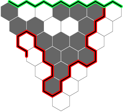
Another way to describe this interface is that we color the counterclockwise arc of ${\partial}D$ from $p_{0}$ to $\zeta$ white and the clockwise arc from $p_{0}$ to $\zeta$ black, and $\beta$ then is the common boundary component between white and black in $\overline{D}$ starting at $p_{0}$ . We will call this type of interface a chordal interface, to differentiate it from the interface that we will later need when discussing the annulus crossing event. (The chordal interface was proved by Smirnov [30] to converge to chordal SLE(6).)

Proof of Theorem 4.1. We mostly concentrate on the case of site percolation on the triangular grid. The details in the case of bond percolation on $\mathbb{Z}^{2}$ are essentially the same.

The algorithm proceeds as follows. (See Figure 4.4.) There are four distinguished boundary arcs of $D$ , which we call “left”, “right”, “up” and “down”. Pick uniformly at random an edge $e_{0}$ on the right hand boundary of $D$ , and let $p_{0}$ be its midpoint. Let $\zeta$ be the union of the top and left boundary segments of $D$ . Explore the interface $\beta$ from $p_{0}$ to $\zeta$ , examining the bits associated to sites in hexagons touching that interface, only as needed to continue with the determination of the interface. Note that the knowledge of $\beta$ suffices to determine if there is an open crossing from the right boundary of $D$ above $p_{0}$ to the left boundary of $D$ : there is such a crossing if and only if $\beta$ terminates on the left boundary of $D$ .

Now let $\zeta^{\prime}$ be the union of the bottom and left boundaries of $D$ , and let $\beta^{\prime}$ be the interface from $p_{0}$ to $\zeta^{\prime}$ that corresponds to the configuration $\omega^{\prime}$ obtained by flipping all the colors of the hexagons in $\overline{D}$ (alternatively, $\beta^{\prime}$ is an interface that has black on the right and white on the left). Then $\beta^{\prime}$ determines the existence of an open crossing from the right boundary below $p_{0}$ to the left boundary. Consequently, after the algorithm examines $\beta$ and $\beta^{\prime}$ , the correct value of $Q$ is determined. We now need to bound the revealment of this algorithm.

Lemma 4.3.

Let ${\partial}_{W}$ denote the counterclockwise arc of ${\partial}D\setminus\zeta$ from $p_{0}$ to $\zeta$ (the white arc), and let ${\partial}_{B}$ denote the clockwise arc of ${\partial}D\setminus\zeta$ from $p_{0}$ to $\zeta$ . Let $H$ be a grid hexagon in $\overline{D}$ . Set $r_{1}:=\min\{\mathop{\mathrm{dist}}(H,{\partial}_{W}),\mathop{\mathrm{dist}}(H,{\partial}_{B})\}$ and $r_{2}:=\max\{\mathop{\mathrm{dist}}(H,{\partial}_{W}),\mathop{\mathrm{dist}}(H,{\partial}_{B})\}$ . Then

{{\bf P}\bigl[{\partial}H\cap\beta\neq\emptyset\bigm|p_{0}\bigr]}\leq\alpha_{2}(r_{1})\,\alpha^{+}\bigl(2\,r_{1}+O(1),r_{2}-r_{1}-O(1)\bigr)\,.

Proof. Suppose that ${\partial}H\cap\beta\neq\emptyset$ . Then there is a path in black hexagons from ${\partial}H$ to ${\partial}_{B}$ and there is a path in white hexagons from ${\partial}H$ to ${\partial}_{W}$ , because the chains of hexagons along the two sides of $\beta$ provide such paths. Suppose, for example, that $r_{1}=\mathop{\mathrm{dist}}(H,{\partial}_{W})$ . Let $w$ be a closest point to $H$ in ${\partial}_{W}$ . Let $M$ be a half space that contains $D$ , which satisfies $\mathop{\mathrm{dist}}({\partial}M,w)\leq C$ where $C=O(1)$ . (Here, we are using the fact that $D$ approximates a convex domain.) Let $w^{\prime}$ be a point closest to $H$ on ${\partial}M$ . Then $\mathop{\mathrm{dist}}(w^{\prime},H)\leq r_{1}+C$ . Set $R_{1}=2\,r_{1}+2\,C+2\mathop{\mathrm{diam}}(H)$ and $R_{2}=r_{2}-r_{1}-C-\mathop{\mathrm{diam}}(H)$ , and assume for now that $R_{2}>R_{1}$ . Consider next the annulus centered at $w^{\prime}$ with inner radius $R_{1}$ and outer radius $R_{2}$ . Now, $M$ intersected with this annulus contains a black crossing between the two boundary circles of this annulus (because there is a black crossing from $H$ to ${\partial}_{B}$ ), and there are black and white crossings between $H$ and the circle of radius $r_{1}$ around the center of $H$ . These events are independent given $p_{0}$ , which implies the lemma in the case $r_{1}=\mathop{\mathrm{dist}}(H,{\partial}_{W})$ , $R_{2}>R_{1}$ . If $R_{2}\leq R_{1}$ and $r_{1}=\mathop{\mathrm{dist}}(H,{\partial}_{W})$ , we only need to consider the crossings between $H$ and the circle of radius $r_{1}$ around its center. The case $r_{1}=\mathop{\mathrm{dist}}(H,{\partial}_{B})$ is treated similarly. ∎

Proof of Theorem 4.1, continued. Fix a hexagon $H\subset\overline{D}$ . Note that the value of $r_{1}$ in the lemma does not depend on $p_{0}$ , since $r_{1}=\mathop{\mathrm{dist}}(H,{\partial}D\setminus\zeta)$ . Let $z_{0}$ be the closest point to $H$ on the right boundary of the square which $D$ approximates. Observe that $r_{2}\geq|p_{0}-z_{0}|-O(1)$ . This implies that for every $r\in[1,R]$ , ${{\bf P}\bigl[r/2\leq r_{2}<r\bigr]}\leq O(r/R)$ . Using the monotonicity of $\alpha^{+}$ , Lemma 4.3 therefore gives

{{\bf P}\bigl[{\partial}H\cap\beta\neq\emptyset\bigr]}\\ \leq O(1)\,\max_{0\leq r_{1}\leq R}\Bigl(\alpha_{2}(r_{1})\sum_{j=0}^{\lceil\log_{2}R\rceil}2^{-j}\alpha^{+}\bigl(2\,r_{1}+O(1),2^{-j}R-r_{1}-O(1)\bigr)\Bigr).

The same estimate also applies to $\beta^{\prime}$ , by symmetry. Consequently, (3.6) gives

{{\bf P}\bigl[H\text{ examined by algorithm}\bigr]}\\ \leq R^{o(1)}\max_{0\leq r_{1}\leq R}\Bigl({r_{1}}^{-1/4}\sum_{j=0}^{\lceil\log_{2}R\rceil}2^{-j}(2^{-j}R/r_{1})^{-1/3}\Bigr)\\ \leq R^{o(1)}\max_{0\leq r_{1}\leq R}\bigl({r_{1}}^{1/12}R^{-1/3}\bigr)=R^{-1/4+o(1)}\,,

as $R\to\infty$ . This proves the theorem in the case of the triangular grid.

The proof for the square grid is essentially the same. Since in that case, we cannot use the values of the critical exponents, we just use the bounds $\alpha^{+}(r,r^{\prime})\leq C\,(r/r^{\prime})^{\epsilon_{0}}$ and $\alpha_{2}(r_{1})\leq C\,r_{1}^{-\epsilon_{0}}$ , which are valid for some constants $C,\epsilon_{0}>0$ . The theorem follows. ∎

We now give the proof of Theorem 1.7. We will not prove Theorem 1.6, but rather simply say that it is proved in a similar way.

Proof of Theorem 1.7. Fix $\gamma<1/8$ . Let $f$ be the indicator function $f(\omega)=1_{A_{m}^{\prime}}(\omega)$ . By (2.1), we have

N(A_{m}^{\prime},m^{-\gamma})=\sum_{\emptyset\neq S\subseteq[n_{m}]}\hat{f}(S)^{2}(1-2\,m^{-\gamma})^{2|S|}

where $n_{m}$ is the number of sites in $D$ . By Corollary 4.2, with $\epsilon>0$ chosen so that $2\,\gamma+\epsilon<1/4$ , this is at most

C\sum_{k=1}^{n_{m}}(1-2m^{-\gamma})^{2k}\,k\,m^{-1/4+\epsilon}\\ \leq C\,{m^{-1/4+\epsilon}}\sum_{k=1}^{\infty}k\,(1-2\,m^{-\gamma})^{\frac{m^{\gamma}}{2}\frac{4k}{m^{\gamma}}}\leq C\,{m^{-1/4+\epsilon}}\sum_{k=1}^{\infty}k\,e^{-4k{m^{-\gamma}}}

It is easy to check that

\sum_{k=1}^{\infty}k\,e^{-4k{m^{-\gamma}}}\leq O(m^{2\gamma})\,,

and so the result follows immediately. ∎

4.2 Annulus case

For the proof of Theorem 1.3, we will need the following variant of Theorem 4.1 regarding the percolation crossings of an annulus.

Theorem 4.4.

Let $2\leq r<R$ . Let $f_{r}^{R}$ be the indicator function for the event that there is a crossing of the annulus $\{z\in\mathbb{R}^{2}:r\leq z\leq R\}$ from the inner circle to the outer circle by a cluster of white hexagons. Then there is a randomized algorithm determining $f_{r}^{R}$ with

\delta\leq r^{o(1)}\,\alpha(r,R)\,\alpha_{2}(r)\,.

(4.1)

We stress that the $r^{o(1)}$ factor depends on $r$ only and not on $R$ . It is possible to replace the factor $r^{o(1)}$ by $O(1)$ , but in order to do this it seems that one would first need to appeal to the analogue of (3.1) for $\alpha_{2}$ , which is proved in the appendix. In order to have a more direct proof of our main theorem, we prefer, at this point, not to rely on the appendix. By (3.4) and (3.5), the right hand side in (4.1) is equal to $R^{-5/48+o(1)}\,r^{-7/48}$ , but its writing in (4.1) is more suggestive and more useful.

Since $\|f_{r}^{R}\|^{2}=\alpha(r,R)$ , Theorems 1.8 and 4.4 give

Corollary 4.5.

\sum_{|S|=k}\hat{f}_{r}^{R}(S)^{2}\leq k\,r^{o(1)}\,\alpha(r,R)^{2}\,\alpha_{2}(r)

holds when $1\leq r<R<\infty$ and $k>0$ . ∎

Before we prove Theorem 4.4, we have to discuss the kind of interface that is used by the algorithm, as it is slightly different from the interface used to determine a possible crossing of a square.

Fix $R>0$ large. Let $\overline{D}=\overline{D}_{R}$ be the union of the hexagons of the hexagonal grid that intersect the disk $|z|\leq R$ . Let $V^{*}=V^{*}_{R}$ denote the set of vertices of the hexagonal grid that are in $\overline{D}$ . Let $p_{0}$ be some point in ${\partial}\overline{D}\setminus V^{*}$ . Let $H_{0}$ denote the hexagon containing the origin, and let $q_{0}$ be some point in ${\partial}H_{0}\setminus V^{*}$ . We define the radial interface $\beta=\beta(R,p_{0},q_{0},\omega)$ , inductively as a simple path from $p_{0}$ to $q_{0}$ . (See Figure 4.5.) The construction is segment by segment, and the concatenation of the first $m$ segments will be denoted $\beta_{m}$ . If the (unique) hexagon in $\overline{D}$ containing $p_{0}$ is white [respectively, black], then the first segment $\beta_{1}$ of $\beta$ traverses the boundary of that hexagon [counter-] clockwise until the first encounter with a point in $V^{*}$ . Suppose inductively $\beta_{m}$ has been constructed, that it is a simple path, that $p_{m}\in V^{*}$ and $p_{0}$ are the two endpoints of $\beta_{m}$ , and that there is a path $\alpha$ in the hexagonal grid in $\overline{D}$ from $p_{m}$ to $q_{0}$ whose only intersection with $\beta_{m}$ is $p_{m}$ . The first step of such a path $\alpha$ is along an edge $\hat{e}$ starting at $p_{m}$ . If there is just one possible $\hat{e}$ among all such $\alpha$ , then $\beta_{m+1}$ also uses that edge $\hat{e}$ . Clearly, there are at most two possible $\hat{e}$ , since the edge terminating at $p_{m}$ and used by $\beta_{m}$ cannot be used. If there are two possible $\hat{e}$ , then $\beta_{m+1}$ chooses between them according to the color of the hexagon containing them both; i.e., the hexagon just encountered by $\beta_{m}$ . If that hexagon is white [respectively, black], then the edge chosen is the one that traverses $H$ [counter-] clockwise. If the edge chosen contains $q_{0}$ , then the path stops at $q_{0}$ and the construction terminates. Otherwise, $\beta_{m+1}$ is defined as the union of $\beta_{m}$ and the chosen continuation edge. This completes the definition of $\beta$ .

It is not hard to verify that for every simple path $\hat{\beta}$ in the hexagonal grid from $p_{0}$ to $q_{0}$ that stays in $\overline{D}$ , the probability that $\beta=\hat{\beta}$ is precisely $2^{-n}$ if $n$ is the number of hexagons in $\overline{D}$ that intersect $\hat{\beta}$ . However, we will not use this fact.

Let $r\in[0,R]$ . We now define a truncated version of $\beta$ , which will suffice, as we will see, to determine $f_{r}^{R}$ . We say that $\beta$ completed a [counter-] clockwise loop at some dual vertex $v\in V^{*}$ if $v$ is visited by $\beta$ and there is a hexagon $H$ containing $v$ and another point $u\in{\partial}H$ , which was visited by $\beta$ prior to $v$ , and the oriented arc of $\beta$ from $u$ to $v$ together with the line segment $[v,u]\subset H$ form a [counter-] clockwise loop surrounding $0$ . Let $\beta^{T}$ denote the initial segment of $\beta$ up to the first time in which $\beta$ completed a counterclockwise loop around $0$ or until it hits $q_{0}$ , if there is no such loop.

Lemma 4.6.

The truncated radial interface $\beta^{T}$ meets the disk $|z|\leq r$ if and only if $f_{r}^{R}=1$ .

Proof. Let $[u,v]$ be an edge in $\beta^{T}$ , with $u$ occuring before $v$ along $\beta$ . We claim that if the hexagon $H$ immediately to the right of $[u,v]$ is contained in $\overline{D}$ , then it is white. Indeed, suppose the contrary. Let $w$ be the first vertex along $\beta$ in which ${\partial}H$ is visited, and let $\beta^{w}$ be the initial segment of $\beta$ from $p_{0}$ to $w$ . Observe that the counterclockwise arc from $w$ to $v$ is a feasible continuation of $\beta^{w}$ , since $\beta$ contains a path from $v$ to $q_{0}$ and there is no other point but $w$ in ${\partial}H\cap\beta^{w}$ . Since we are assuming that $H\subset\overline{D}$ is black, it follows that the immediate continuation of $\beta^{w}$ was along ${\partial}H$ in the counterclockwise direction until some $w^{\prime}\in V^{*}$ is hit.

Consider the directed cycle obtained by joining the line segment $[u,w^{\prime}]$ to the arc of $\beta$ from $w^{\prime}$ to $u$ . This directed cycle surrounds $v$ , because $w$ is connected in $\beta^{w}$ to $p_{0}$ , which is certainly in the unbounded component of this cycle, and the line segment $[v,w]$ intersects the cycle precisely once, crossing the line segment $[u,w^{\prime}]$ inside $H$ . Moreover, if we consider the orientation in which these two line segments cross, we conclude that the cycle surrounds $v$ counterclockwise. Because the arc of $\beta$ from $v$ to $q_{0}$ does not intersect the cycle, we conclude that the cycle also surrounds $0$ counterclockwise. This contradicts the definition of the truncated path $\beta^{T}$ , since we are assuming $v\in\beta^{T}$ . This verifies our claim, that to the right of edges in $\beta^{T}$ are only white hexagons and hexagons that are not contained in $\overline{D}$ .

Note that if $e$ and $e^{\prime}$ are two consecutive segments along $\beta$ , then the hexagon to the right of $e$ is either the same as the one to the right of $e^{\prime}$ , or these hexagons are adjacent. We therefore conclude that every white hexagon visited by $\beta^{T}$ is connected by a chain of white hexagons to ${\partial}D$ . Therefore, if $\beta^{T}$ hits the set $|z|\leq r$ , then clearly $f_{r}^{R}=1$ .

Now suppose that $\beta^{T}$ does not hit $|z|\leq r$ . This implies that $\beta^{T}$ has terminated by completing a counterclockwise loop around the set $|z|\leq r$ . Consider a hexagon $H$ on the inner boundary of this loop. Because the orientation of the loop is counterclockwise, the first time in which $H$ is visited, the path chose to traverse ${\partial}H$ counterclockwise. This implies that the hexagon is black. Thus, there is a loop of black hexagons in $\overline{D}$ that surrounds the set $|z|\leq r$ . This implies that $f_{r}^{R}=0$ . ∎

We can now specify the algorithm promised by Theorem 4.4. The algorithm starts by selecting the point $p_{0}$ uniformly along ${\partial}\overline{D}$ , and selecting $q_{0}$ arbitrarily in ${\partial}H_{0}\setminus V^{*}$ . It then proceeds to inspect the colors of the hexagons necessary to develop the truncated interface $\beta^{T}$ , until it terminates or hits the set $|z|\leq r$ . At that point, the correct value of $f_{r}^{R}$ is determined, by Lemma 4.6.

In order to bound the revealment of this algorithm, it will be convenient to introduce a different interface, which in the end will turn out to be equivalent to $\beta$ .

Let $\hat{D}$ denote the branched double cover of $\overline{D}$ about $0$ , and let $\phi:\hat{D}\to\overline{D}$ denote the projection map. Concretely, define $\hat{D}$ as the preimage of $\overline{D}$ under the map $\phi(z)=z^{2}$ . Let $\hat{p}_{0}$ be one of the preimages of $p_{0}$ under $\phi$ , and let $\hat{q}_{0}$ be one of the preimages of $q_{0}$ . Let $\hat{H}_{0}$ be the closure of one of the connected components of $\phi^{-1}(H_{0})\setminus[\hat{q}_{0},-\hat{q}_{0}]$ . Let $\mathfrak{H}$ denote the set of hexagons $H$ that are contained in $\overline{D}$ . Let $\hat{\mathfrak{H}}$ denote the set of connected components of preimages $\phi^{-1}(H)$ , $H\in\mathfrak{H}$ , except that the single preimage of $H_{0}$ is replaced by the two sets $\hat{H}_{0}$ and $-\hat{H}_{0}$ . Note that if $\hat{H}\in\hat{\mathfrak{H}}$ , then $-\hat{H}\in\hat{\mathfrak{H}}$ and $\phi(\hat{H})=\phi(-\hat{H})\in\mathfrak{H}$ . Let $\hat{\mathfrak{H}}^{\prime}\subset\hat{\mathfrak{H}}$ be a maximal collection of elements of $\hat{\mathfrak{H}}$ with the property that $\hat{\mathfrak{H}}^{\prime}\cap\{-\hat{H}:\hat{H}\in\hat{\mathfrak{H}}^{\prime}\}=\emptyset$ . Now color at random each of the elements of $\hat{\mathfrak{H}}^{\prime}$ white or black independently, with probability $1/2$ . For every $\hat{H}\in\hat{\mathfrak{H}}^{\prime}$ , let $-\hat{H}$ have the opposite color to the color of $\hat{H}$ .

Now let $\hat{\beta}$ denote the chordal interface in $\hat{D}$ from $\hat{p}_{0}$ to $-\hat{p}_{0}$ , with white cells on the right and black cells on the left, as defined in the simply connected setting in Subsection 4.1. That is, we consider the exterior of the counterclockwise arc from $\hat{p}_{0}$ to $-\hat{p}_{0}$ along ${\partial}\hat{D}$ as white, the exterior of the complementary arc as black, and take $\hat{\beta}$ as the interface between white and black passing through $\hat{p}_{0}$ and through $-\hat{p}_{0}$ . Finally, let $\beta^{\dagger}:=\phi(\hat{\beta})\setminus\operatorname{interior}(H_{0})$ .

Lemma 4.7.

Given $p_{0}$ and $q_{0}$ , the laws of $\beta^{\dagger}$ and of $\beta$ are the same.

(In this statement, we consider $\beta$ as a set, and forget about the fact that it has the structure of an oriented path.)

Proof. The map $z\mapsto-z$ preserves $\hat{\beta}$ , by the symmetry of the interface. Consequently, near every point $p\in\beta^{\dagger}\setminus\{p_{0},q_{0}\}$ , $\beta^{\dagger}$ looks like a piecewise linear path. Moreover, $\beta^{\dagger}$ is connected and contains $p_{0}$ . Since a compact simple path has two endpoints, we conclude that $q_{0}\in\beta^{\dagger}$ as well. We now consider building $\beta^{\dagger}$ by adding one segment at a time. When it hits a previously unvisited hexagon $H$ which is contained in $\overline{D}$ , it is equally likely (given its past) to turn right or left. (This is because both preimages of $H$ are unvisited by both preimages of the past of $\beta^{\dagger}$ .) When it hits a previously visited hexagon (or a hexagon that is not contained in $\overline{D}$ ), it turns in such a way that it will eventually be able to reach $q_{0}$ without crossing itself, and this uniquely specifies this turn. Consequently, the lemma follows. ∎

Remark 4.8.

The radial interface converges to radial SLE(6) as the mesh tends to zero.

Proof of Theorem 4.4. Given all of our preparations, the proof is rather easy. We have shown that the above algorithm provides the correct answer. It therefore remains to estimate its revealment. Consider some hexagon $H\subset\overline{D}$ . We want to prove that the right hand side of (4.1) is an upper bound for the probability that $H$ is examined. Let $a:=\mathop{\mathrm{dist}}(0,H)$ , $b:=\mathop{\mathrm{dist}}(H,{\partial}\overline{D})$ and $c:=\mathop{\mathrm{dist}}(p_{0},H)$ . Let $S_{1}$ be the disk of radius $(a\wedge b)/2$ concentric with $H$ , and let $\hat{S}_{1}$ be one of the two connected components of $\phi^{-1}(S_{1})$ . We have to bound the probability that the algorithm inspects $H$ . Clearly, we may assume $a\geq r-O(1)$ . For $H$ to be inspected, $\beta^{T}$ has to get to the circle $|z|=R\wedge(2\,a)$ . This probability is $\alpha(2\,a,R)$ . Given that this has happened, how can we estimate the probability that $\beta$ is adjacent to $H$ ? At this point, we use the equivalence of $\beta$ and $\beta^{\dagger}$ . The information that $\beta^{\dagger}$ reached the circle $|z|=R\wedge(2\,a)$ bears no impact on the distribution of the colors of the cells in $\hat{\mathfrak{H}}$ whose images under $\phi$ intersect $S_{1}$ . (Here, we assume that $a$ is not too small, so that the corresponding sets of cells are disjoint. Certainly $a>10$ suffices. If $a$ is smaller, then the estimate we are now striving for is trivial.) Since there is no hexagon intersecting both $\hat{S}_{1}$ and $-\hat{S}_{1}$ , it follows that the conditional distribution of the colors of the cells meeting $\hat{S}_{1}$ is uniform i.i.d. Consequently, the conditional probability that $\beta^{\dagger}$ hits $H$ is bounded by $\alpha_{2}((a\wedge b)/2)$ . Thus,

{{\bf P}\bigl[H\text{ visited}\bigr]}\leq O(1)\,\alpha(2\,a,R)\,\alpha_{2}((a\wedge b)/2)\,.

In the case $b\geq a\geq 2\,r$ , we may use independence on disjoint sets to conclude that

		$\displaystyle\bf{{\displaystyle P}\bigl[H\text{ visited}\bigr]}$
		$\displaystyle\leq O(1)\,\alpha_{2}(r)\,\alpha_{2}(2\,r,a/2)\,\alpha(2\,a,R)\leq O(1)\,\alpha_{2}(r)\,\alpha(2\,r,a/2)\,\alpha(2\,a,R)$
		$\displaystyle\overset{(\ref{e.rsw})}{\leq}O(1)\,\alpha_{2}(r)\,\alpha(r,2\,r)\,\alpha(2\,r,a/2)\,\alpha(a/2,2\,a)\,\alpha(2\,a,R)$
		$\displaystyle\overset{(\ref{e.multip})}{\leq}O(1)\,\alpha_{2}(r)\,\alpha(r,R)\,.$

On the other hand, if $b\geq a$ and $a\leq 2\,r$ , then we use our assumption $a\geq r-O(1)$ and (3.5) to get $\alpha_{2}(a/2)\leq r^{-1/4+o(1)}\leq\alpha_{2}(r)\,r^{o(1)}$ , which is also sufficient.

In the case $b<a$ , a similar argument (and similar to the proof of Lemma 4.3) shows that

{{\bf P}\bigl[H\text{ visited }\bigm|c\bigr]}\leq O(1)\,\alpha_{2}(b/2)\,\alpha^{+}\bigl(2\,b+O(1),c-b-O(1)\bigr).

Next, picking a constant $q\in(1/4,1/3)$ , we then have by the above and (3.6)

{{\bf P}\bigl[H\text{ visited }\bigm|c\bigr]}\leq O(1)\,\alpha_{2}(b/2)\,(c/b)^{-q}.

As in the proof of Theorem 4.1, we have ${{\bf P}\bigl[2^{j}\leq c<2^{j+1}\bigr]}\leq O(1)\,2^{j}/R$ . It easily follows that

{{\bf P}\bigl[H\text{ visited}\bigr]}\leq O(1)\,\alpha_{2}(b/2)\,(R/b)^{-q}.

If $b/2>r$ , then we may estimate

\alpha_{2}(b/2)\leq\alpha_{2}(r)\,\alpha_{2}(2\,r,b/2)\leq\alpha_{2}(r)\,\alpha(2\,r,b/2)

and

(R/b)^{-q}\overset{(\ref{e.expostrong})}{\leq}O(1)\,\alpha(b/2,R)

and we get from (3.1) and the above

{{\bf P}\bigl[H\text{ visited}\bigr]}\leq O(1)\,\alpha_{2}(r)\,\alpha(r,R)\,.

If $b/2\leq r$ , we use instead

\alpha_{2}(b/2)\,(R/b)^{-q}\leq O(1)\,\alpha_{2}(b/2)\,\alpha_{2}(b/2,r)\,\alpha(r,R)\overset{(\ref{e.expostrong})}{\leq}r^{o(1)}\,\alpha_{2}(r)\,\alpha(r,R)\,.

This completes the proof. ∎

Remark 4.9.

It is easy to see that if we assume the analogue of (3.1) for $\alpha_{2}$ proved in the appendix, then the $r^{o(1)}$ term in (4.1) can be replaced by $O(1)$ .

5 Exceptional times

In this section we prove Theorem 1.3. We point out that the absolute key necessary step is to get a good bound on the correlation for an event occurring at two different but close by times. Once this is done, the rest is fairly standard. Proposition A16 in Lawler [22] indicates this general type of argument.

Proof of Theorem 1.3. By Kolmogorov’s 0-1 law, it suffices to prove that with positive probability there are times in $[0,1]$ when the origin is in an infinite cluster. Fix $R>2$ large and let $V_{t,R}$ be the event that at time $t$ there is an open path from the origin to distance $R$ away. We then let

X=X_{R}:=\int_{0}^{1}1_{V_{t,R}}\,dt

be the Lebesgue measure of the set of times in $[0,1]$ at which $V_{t,R}$ occurs. The first moment of $X$ is given by

{{\bf E}\bigl[X\bigr]}=\int_{0}^{1}{{\bf P}\bigl[V_{t,R}\bigr]}\,dt={{\bf P}\bigl[V_{0,R}\bigr]}=\alpha(R)\,.

The second moment is

{{\bf E}\bigl[X^{2}\bigr]}={{\bf E}\Bigl[\int_{0}^{1}\int_{0}^{1}1_{V_{s,R}}\,1_{V_{s^{\prime},R}}\,ds\,ds^{\prime}\Bigr]}=\int_{0}^{1}\int_{0}^{1}{{\bf P}\bigl[V_{s,R}\cap V_{s^{\prime},R}\bigr]}\,ds\,ds^{\prime}.

(5.1)

For each site $v$ we let

\chi_{v}^{s}:=\begin{cases}-1&v\text{ is open at time }s\\ 1&\text{otherwise},\end{cases}

and for a finite set of sites $S$ set

\chi_{S}^{s}:=\prod_{v\in S}\chi_{v}^{s}\,.

Fix $s,s^{\prime}\in[0,1]$ , and set $t:=|s-s^{\prime}|$ . Recall that the state of a site $v$ flips between closed and open with rate $1/2$ . Equivalently, we may think of the state as being re-randomized with rate $1$ . Consequently, ${{\bf P}\bigl[\chi_{v}^{s^{\prime}}=\chi_{v}^{s}\bigm|\omega_{s}\bigr]}=e^{-t}+(1-e^{-t})/2=(1+e^{-t})/2$ , and hence,

{{\bf E}\bigl[\chi_{v}^{s}\,\chi_{v}^{s^{\prime}}\bigr]}=\exp(-t)\,,\qquad{{\bf E}\bigl[\chi_{S}^{s}\,\chi_{S}^{s^{\prime}}\bigr]}=\prod_{v\in S}{{\bf E}\bigl[\chi_{v}^{s}\,\chi_{v}^{s^{\prime}}\bigr]}=\exp(-t\,|S|)\,.

Moreover, if $S\neq S^{\prime}$ , then ${{\bf E}\bigl[\chi_{S}^{s}\,\chi_{S^{\prime}}^{s^{\prime}}\bigr]}=0$ . Consequently, if $f$ is a function depending on the states of finitely many lattice points and has the expansion $f(\omega)=\sum_{S}\hat{f}(S)\,\chi_{S}(\omega)$ , then

{{\bf E}\bigl[f(\omega_{s})\,f(\omega_{s^{\prime}})\bigr]}=\sum_{S}\hat{f}(S)^{2}\exp(-t\,|S|)\,.

(5.2)

Let $f_{r}^{R}(\omega)$ be as in Theorem 4.4. Fix some $t\in(0,1]$ and let $r\in[2,R)$ . Clearly, $0\leq f_{0}^{R}(\omega)\leq f_{0}^{r}(\omega)\,f_{2r}^{R}(\omega)$ for every $\omega$ . Consequently,

{{\bf P}\bigl[V_{s,R}\cap V_{s^{\prime},R}\bigr]}={{\bf E}\bigl[f_{0}^{R}(\omega_{s})\,f_{0}^{R}(\omega_{s^{\prime}})\bigr]}\leq{{\bf E}\bigl[f_{0}^{r}(\omega_{s})\,f_{2r}^{R}(\omega_{s})\,f_{0}^{r}(\omega_{s^{\prime}})\,f_{2r}^{R}(\omega_{s^{\prime}})\bigr]}\\ ={{\bf E}\bigl[f_{0}^{r}(\omega_{s})\,f_{0}^{r}(\omega_{s^{\prime}})\bigr]}{{\bf E}\bigl[f_{2r}^{R}(\omega_{s})\,f_{2r}^{R}(\omega_{s^{\prime}})\bigr]}\leq{{\bf E}\bigl[f_{0}^{r}(\omega_{s})\bigr]}{{\bf E}\bigl[f_{2r}^{R}(\omega_{s})\,f_{2r}^{R}(\omega_{s^{\prime}})\bigr]}.

(To obtain the second equality, we have used the independence on disjoint sets of sites.) Thus,

{{\bf P}\bigl[V_{s,R}\cap V_{s^{\prime},R}\bigr]}\leq\alpha(r)\,{{\bf E}\bigl[f_{2r}^{R}(\omega_{s})\,f_{2r}^{R}(\omega_{s^{\prime}})\bigr]}=\alpha(r)\,\sum_{S}e^{-t|S|}\hat{f}_{2r}^{R}(S)^{2}.

The latter sum restricted to $S$ with $|S|=k$ for fixed $k\neq 0$ is estimated using Corollary 4.5, while for $k=0$ , we use $\hat{f}_{2r}^{R}(\emptyset)=\alpha(2r,R)$ . This yields

{{\bf P}\bigl[V_{s,R}\cap V_{s^{\prime},R}\bigr]}\leq\alpha(r)\,\Bigl(\alpha(2\,r,R)^{2}+r^{o(1)}\,\sum_{k=1}^{\infty}e^{-kt}k\,\alpha(2\,r,R)^{2}\,\alpha_{2}(r)\Bigr).

It is easy to check that $\sum_{k=1}^{\infty}k\,e^{-kt}\leq O(t^{-2})$ . This and the inequalities (3.1) and (3.2) allow us to write this estimate as

{{\bf P}\bigl[V_{s,R}\cap V_{s^{\prime},R}\bigr]}\leq O(1)\,\alpha(R)^{2}\,\alpha(r)^{-1}\bigl(1+r^{o(1)}\,t^{-2}\,\alpha_{2}(r)\bigr)\,.

(5.3)

We proved the above claim for all $t\in(0,1]$ and $r\in[0,R)$ but now we observe that (5.3) is also trivially true when $r\geq R$ as well. We now choose $r=2\,t^{-8}=2\,|s-s^{\prime}|^{-8}$ . Applying this in (5.3) with (3.3) and (3.5) gives

{{\bf P}\bigl[V_{s,R}\cap V_{s^{\prime},R}\bigr]}\leq O(1)\,\alpha(R)^{2}\,|s-s^{\prime}|^{-5/6+o(1)}.

(5.4)

Hence,

\int_{0}^{1}\int_{0}^{1}{{\bf P}\bigl[V_{s,R}\cap V_{s^{\prime},R}\bigr]}\,ds\,ds^{\prime}\leq O(1)\,\alpha(R)^{2}.

(5.5)

The Cauchy-Schwarz inequality tells us that

{{\bf P}\bigl[X>0\bigr]}\geq\frac{{{\bf E}\bigl[X\bigr]}^{2}}{{{\bf E}\bigl[X^{2}\bigr]}}\,.

Consequently, the above inequality, the fact that ${{\bf E}\bigl[X\bigr]}=\alpha(R)$ , the expression (5.1) for ${{\bf E}\bigl[X^{2}\bigr]}$ and (5.5) show that $\inf_{R>0}{{\bf P}\bigl[X_{R}>0\bigr]}>0$ . Let $T_{R}:=\{t\in[0,1]:V_{t,R}\text{ holds}\}$ . Fatou’s lemma tells us that with positive probability $T_{R}\neq\emptyset$ for infinitely many $R\in\mathbb{N}$ . Since $T_{R}\supset T_{R^{\prime}}$ when $R^{\prime}>R$ , this implies that

{{\bf P}\bigl[\cap_{R>0}\,\,\{T_{R}\neq\emptyset\}\bigr]}>0.

Our goal is to show that ${{\bf P}\bigl[\bigcap_{R}T_{R}\neq\emptyset\bigr]}>0$ . Since the $T_{R}$ ’s are not closed sets, $\cap_{R>0}\,\,\{T_{R}\neq\emptyset\}$ does not immediately imply $\bigcap_{R}T_{R}\neq\emptyset$ . (The reason that $T_{R}$ is not necessarily closed is that the set of times at which an edge is open is not a closed set since we have a right continuous process.) This technicality is taken care of by the following lemma from [13].

Lemma 5.1.

([13]) Let $0<p<1$ and let $G$ be any graph where $\pi_{p}({\cal C})=0$ . Let $\{\omega_{t}\}$ represent our dynamical percolation process in that $\omega_{t}(v)$ is the state of vertex $v$ at time $t$ . Consider the process $\{\bar{\omega}_{t}\}$ obtained from $\{\omega_{t}\}$ by setting, for every vertex $v$ , the set $\{t\,:\,\bar{\omega}_{t}(v)=1\}$ to be the closure of the set $\{t\,:\,\omega_{t}(v)=1\}$ . Then $\mbox{\boldmath$\Psi$}_{p}$ -a.s., for every vertex $v$ we have

\{t\in[0,\infty)\>:\>v\,\mbox{ \rm percolates in }\bar{\omega}_{t}\}\,=\,\{t\in[0,\infty)\>:\>v\,\mbox{ \rm percolates in }\omega_{t}\}\,.

In particular, a.s. this set of times is closed.

Returning to our proof, let $\overline{T_{R}}$ be the closure of $T_{R}$ . It is easily checked that

\bigcap_{R>0}\overline{T_{R}}=\{t\in[0,1]\>:\>0\,\mbox{ \rm percolates in }\bar{\omega}_{t}\},

where $\{\bar{\omega}_{t}\}$ is defined in Lemma 5.1. By compactness, if the $T_{R}$ ’s are all nonempty, it follows that $\bigcap_{R}\overline{T_{R}}$ is nonempty. This implies that there is some time at which $\bar{\omega}_{t}$ percolates and hence by Lemma 5.1, some time at which the original process $\omega_{t}$ percolates. ∎

For future reference, we note that Lemma 5.1 implies that a.s.

{\bigcap_{R>0}\overline{T_{R}}=\bigcap_{R>0}{T_{R}}}.

(5.6)

6 Hausdorff dimension of exceptional times

In this section, we prove Theorem 1.9. This is separated into two theorems, Theorem 6.1 and Theorem 6.3, where lower and upper bounds are given. We point out however that the lower bound is simply a refinement of the argument for proving that there exist exceptional times. First note that the fact that the Hausdorff dimension is an almost sure constant follows immediately from ergodicity.

Theorem 6.1.

A.s., the Hausdorff dimension of the set of exceptional times is at least $1/6$ .

Proof. Fix $\gamma<1/6$ . It suffices by ergodicity and countable additivity to show that with positive probability, the set of exceptional times in $[0,1]$ at which the origin percolates has Hausdorff dimension at least $\gamma$ . For each integer $R$ , let as before $V_{t,R}$ be the event that at time $t$ there is a path from the origin to distance $R$ away and define a random measure $\sigma_{R}$ on $[0,1]$ by

\sigma_{R}(S)=\frac{1}{\alpha(R)}\int_{S}1_{V_{t,R}}dt

for each Borel set $S\subset[0,1]$ .

The results in the previous section immediately give that ${\bf E}[\|\sigma_{R}\|]=1$ and ${\bf E}[\|\sigma_{R}\|^{2}]\leq O(1)$ where $\|\sigma_{R}\|$ denotes the total variation of the measure $\sigma_{R}$ .

Cauchy-Schwarz gives

{{\bf E}\bigl[\|\sigma_{R}\|^{2}\bigr]}^{1/2}\,{{\bf P}\bigl[\|\sigma_{R}\|>1/2\bigr]}^{1/2}\geq{{\bf E}\bigl[\|\sigma_{R}\|1_{\|\sigma_{R}\|>1/2}\bigr]}\geq{{\bf E}[\|\sigma_{R}\|]}-1/2=1/2.

Consequently, ${{\bf P}\bigl[\|\sigma_{R}\|>1/2\bigr]}\geq C_{1}$ for some constant $C_{1}>0$ . Given a measure $m$ on $[0,1]$ and $\gamma>0$ , let

{\cal E}_{\gamma}(m)=\int\!\!\int{|t-s|}^{-\gamma}\,dm(t)\,dm(s).

Note that

{{\bf E}\bigl[{\cal E}_{\gamma}(\sigma_{R})\bigr]}={{\bf E}\Bigl[\int_{0}^{1}\!\int_{0}^{1}\frac{d\sigma_{R}(t)\,d\sigma_{R}(s)}{{|t-s|}^{\gamma}}\Bigr]}=\int_{0}^{1}\!\int_{0}^{1}\frac{{{\bf P}\bigl[{V_{t,R}}\cap{V_{s,R}}\bigr]}}{{\alpha(R)^{2}}\,|t-s|^{\gamma}}\,dt\,ds\,.

Therefore, by (5.4) and $\gamma<1/6$ ,

C_{2}:=\sup_{R}{{\bf E}\bigl[{\cal E}_{\gamma}(\sigma_{R})\bigr]}<\infty\,.

By Markov’s inequality, for all $R$ and for all $T$ ,

{{\bf P}\bigl[{\cal E}_{\gamma}(\sigma_{R})\geq C_{2}T\bigr]}\leq 1/T.

Choose $T$ so that $1/T<C_{1}/2$ . Letting

U_{R}=\{\|\sigma_{R}\|>1/2\}\cap\{{\cal E}_{\gamma}(\sigma_{R})\leq C_{2}T\},

by the choice of $T$ , we have that

{{\bf P}\bigl[U_{R}\bigr]}\geq C_{1}/2.

By Fatou’s lemma,

{{\bf P}\bigl[\limsup_{R\to\infty}U_{R}\bigr]}\geq C_{1}/2.

We now show that on the event $\limsup_{R}U_{R}$ , the Hausdorff dimension of the set of percolating times in $[0,1]$ is at least $\gamma$ . Let $\overline{T_{R}}$ again be the closure of the set of times in $[0,1]$ at which there is a path from the origin to distance $R$ away. Clearly $\sigma_{R}$ is supported on $\overline{T_{R}}$ . By (5.6), it suffices to prove that $\bigcap_{R>0}\overline{T_{R}}$ has Hausdorff dimension at least $\gamma$ on the event $\limsup_{R}U_{R}$ . This is achieved in the following (deterministic) lemma, which completes the proof. ∎

Lemma 6.2.

Let $D_{1}\supseteq D_{2}\supseteq D_{3}\ldots$ be a decreasing sequence of compact subsets of $[0,1]$ , and let $\mu_{1},\mu_{2},\dots$ be a sequence of positive measures with $\mu_{n}$ supported on $D_{n}$ . Suppose that there is a constant $C$ such that for infinitely many values of $n$ , we have

\|\mu_{n}\|>1/C,\quad\text{ and }\quad{\cal E}_{\gamma}(\mu_{n})\leq C.

(6.1)

Then the Hausdorff dimension of $\bigcap_{n}D_{n}$ is at least $\gamma$ .

Proof. Choose a sequence of integers $\{n_{k}\}$ for which (6.1) holds. Note that $\|\mu_{n_{k}}\|^{2}\leq\mathcal{E}_{\gamma}(\mu_{n_{k}})\leq C$ . By compactness, choose a further subsequence $\{n^{\prime}_{k}\}$ of $\{n_{k}\}$ so that $\mu_{n^{\prime}_{k}}$ converges weakly to some positive measure $\mu_{\infty}$ . Clearly $\mu_{\infty}$ is supported on $\bigcap_{n}D_{n}$ and $\|\mu_{\infty}\|\geq 1/C$ . For all $M$ , we have that

\int\!\!\int{|x-y|}^{-\gamma}\wedge M\,d\mu_{\infty}(x)\,d\mu_{\infty}(y)=\\ \lim_{k\to\infty}\int\!\!\int{|x-y|}^{-\gamma}\wedge M\,d\mu_{n^{\prime}_{k}}(x)\,d\mu_{n^{\prime}_{k}}(y)\leq C.

Now let $M\to\infty$ and apply the monotone convergence theorem to conclude that

\int\!\!\int{|x-y|}^{-\gamma}\,d\mu_{\infty}(x)\,d\mu_{\infty}(y)\leq C.

Since $\|\mu_{\infty}\|>0$ , it now follows from Frostman’s theorem (see for example, [17]) that the Hausdorff dimension of $\bigcap_{n}D_{n}$ is at least $\gamma$ . ∎

Theorem 6.3.

A.s., the Hausdorff dimension of the set of exceptional times is at most $31/36$ .

Proof. Let $U_{n}$ be the event that there is a time in $[0,1/n]$ for which the origin percolates. Since the set of vertices which are open for some $t\in[0,1/n]$ is an i.i.d. process with density $1/2+(1-e^{-1/(2n)})/2\leq 1/2+1/n$ , it is immedate that

{{\bf P}\bigl[U_{n}\bigr]}\leq\pi_{\frac{1}{2}+\frac{1}{n}}({\cal C}_{0}),

where ${\cal C}_{0}$ is the event that the origin percolates. By page 3 of [31], for every $\epsilon>0$ , there is a $C$ so that

\pi_{\frac{1}{2}+\frac{1}{n}}({\cal C}_{0})\leq C\,n^{\epsilon-5/36}.

(6.2)

Now let

N_{n}=\sum_{j=1}^{n}1_{U_{j,n}}\,,

where $U_{j,n}$ is the event that there is a time in $[(j-1)/n,j/n]$ for which the origin percolates (so $U_{1,n}=U_{n}$ above). By the above, we have that ${{\bf E}\bigl[N_{n}\bigr]}\leq Cn^{\frac{31}{36}+\epsilon}$ . It follows that

\lim_{n}\frac{{{\bf E}\bigl[N_{n}\bigr]}}{n^{\frac{31}{36}+2\epsilon}}=0

and so from Fatou’s lemma, we get

{{\bf E}\Bigl[\liminf_{n}\frac{N_{n}}{n^{\frac{31}{36}+2\epsilon}}\Bigr]}=0.

Therefore

\liminf_{n}\frac{N_{n}}{n^{\frac{31}{36}+2\epsilon}}=0

a.s. This says that a.s. for infinitely many $n$ , the set of exceptional times in $[0,1]$ at which the origin percolates can be covered by $n^{\frac{31}{36}+2\epsilon}$ intervals of length $1/n$ . Hence, the Hausdorff dimension of the set of these exceptional times is at most $\frac{31}{36}+2\epsilon$ a.s. By countable additivity, we are done. ∎

Remark 6.4.

The upper bound will be proved again by a different argument when we prove Theorem (1.16). The above proof is included here, because it is shorter. One should nonetheless point out that the above argument uses (6.2), while the argument below is more self contained.

7 Exceptional times for $k$ -arm events

In this section, we give the proofs of the lower bounds in Theorems 1.15 and 1.16, but generally omit those details which are the same as in the corresponding proofs of Theorems 1.3 and 6.1.

For $\theta>0$ and integer $k\geq 1$ , let $A_{W_{\theta}}^{k}(r,R)$ be the event that we have $k$ disjoint crossings of alternating colors (with black most clockwise) between distances $r$ and $R$ of the origin in $W_{\theta}$ and let $\alpha_{W_{\theta}}^{k}(r,R)={{\bf P}\bigl[A_{W_{\theta}}^{k}(r,R)\bigr]}$ . If $r$ is suppressed, then it is taken to be $10\,k$ .

We will, of course, need the asymptotics of $\alpha_{W_{\theta}}^{k}(r,R)$ . For this purpose, conformal invariance will be used. Although when $\theta>2\pi$ the surface $W_{\theta}$ is not planar and conformal invariance is usually stated for planar domains, the proof of conformal invariance certainly holds in this setting. The asymptotic decay as $R/r\to\infty$ of the probability of $k$ disjoint crossings between distances $r$ and $R$ in $W_{\theta}$ from the origin in the percolation scaling limit is determined using conformal invariance. Specifically, the map $z\mapsto z^{\pi/\theta}$ maps $W_{\theta}$ to the upper half plane, and we may conclude from (3.8) that the decay (for the percolation scaling limit) is of the form $(R/r)^{\frac{-\pi k(k+1)}{6\theta}+o(1)}$ , as $R/r\to\infty$ while $k$ stays fixed. Then, one can conclude, as for the other exponents we have discussed, that for $R\geq r\geq 10\,k$ ,

\alpha_{W_{\theta}}^{k}(r,R)=(R/r)^{\frac{-\pi k(k+1)}{6\,\theta}+o(1)},

(7.1)

as $R/r\to\infty$ while $k$ is fixed, using the argument given in [31]. We will also use the fact that the quasi-multiplicativity relations (3.1) and (3.2) hold for $\alpha_{W_{\theta}}^{k}$ and for $\alpha_{2}$ . This is proved in the appendix; see Remark A.6.

Proof of lower bound in Theorem 1.15. We first handle the case $k=1$ and therefore abbreviate temporarily $\alpha_{W_{\theta}}^{1}(r,R)$ by $\alpha_{W_{\theta}}(r,R)$ . (A different approach will be needed for $k\geq 2$ .) Let $D$ be the union of the hexagons in $W_{\theta}$ that contain points whose distance from the origin is in $[r,R]$ . Let ${\partial}_{R}D$ and ${\partial}_{r}D$ denote the set of points in ${\partial}D$ that are at distance $\geq R$ [respectively, $\leq r$ ] from the origin. Also, we denote by ${\partial}^{0}D$ and ${\partial}^{\theta}D$ , the components of ${\partial}D\cap{\partial}W_{\theta}$ that are at angle about $0$ [respectively, about $\theta$ ] in radial coordinates on $W_{\theta}$ .

The algorithm we use to determine if there exists a crossing of $D$ is essentially the same as the algorithm determining the existence of a left to right crossing of a square, where ${\partial}_{R}D$ plays the role of the right side of the square and where ${\partial}_{r}D$ plays the role of the left side of the square. (This is of course crucial; if we reversed things, then the hexagons near the inner circle would be revealed with too high of a probability.) It is clear that this algorithm works and so we now need to compute its revealment. We will show that the revealment is

O(1)\,\alpha_{2}(r)\,\alpha_{W_{\theta}}(r,R)\,.

(7.2)

Using (7.1) and (3.6), one can show that this is essentially (i.e., up to some $O(1)$ factor) monotone decreasing in $r$ in the relevant range $\theta>8\,\pi/3$ .

We just look at the first interface arising in the algorithm, the one which terminates when it hits ${\partial}_{r}D\cup{\partial}^{\theta}D$ , since the estimates for the second interface will be essentially the same.

Fix some hexagon $H\subset D$ . Let $s=\mathop{\mathrm{dist}}(H,{\partial}_{R}D\cup{\partial}^{0}D\cup\{0\})$ with $0$ denoting the origin. We also use $|p|$ to denote distance from $0$ in $W_{\theta}$ . We distinguish several different cases.

Case 1: $\mathop{\mathrm{dist}}(H,\{0\})=s$ . For $H$ to be visited, we need our 2 arms event holding within distance $s/2$ of $H$ and a crossing of the desired color between distance $2s$ and distance $R$ from the origin. These are independent and we get that $H$ is visited with probability at most $\alpha_{2}(s/2)\,\alpha_{W_{\theta}}(2s,R)$ . By the analogues of (3.1) and (3.2) for $\alpha_{2}$ and $\alpha_{W_{\theta}}$ , this is compatible with our claimed revealment (7.2).

Case 2: $\mathop{\mathrm{dist}}(H,{\partial}_{R}D)=s$ . As in the proof of Theorem 4.4 with $c:=\mathop{\mathrm{dist}}(p_{0},H)\wedge(R/2)$ , we obtain

{{\bf P}\bigl[H\text{ visited }\bigm|p_{0}\bigr]}\leq O(1)\,\alpha^{+}(2s+O(1),c-s-O(1))\,\alpha_{2}(s/2).

Proceeding as in that proof, this is also compatible with our claimed revealment (7.2).

Case 3: $\mathop{\mathrm{dist}}(H,{\partial}^{0}D)=s$ . Let $w\in{\partial}^{0}D$ so that $\mathop{\mathrm{dist}}(H,w)=s$ . We separate Case 3 into 3 subcases.

Case 3(a): $s\geq|w|/2$ . Then the triangle inequality gives $\mathop{\mathrm{dist}}(H,0)\leq 3s$ . For $H$ to be visited, we need our 2 arms event holding within distance $s/2$ of $H$ and a path of the desired type between distance $4s$ and distance $R$ from the origin. These are independent and we get that $H$ is visited with probability at most $\alpha_{2}(s/2)\,\alpha_{W_{\theta}}(3s,R)$ , which is compatible with our claimed revealment 7.2.

Case 3(b): $s\leq|w|/2\leq R/4$ . For $H$ to be visited, we need our 2 arms event holding within distance $s/2$ of $H$ , a white crossing in the half annulus centered at $w$ with outer radius $|w|$ and inner radius $2s$ (which is identical to a half-annulus in a half-plane; $|w|\leq R/2$ guarantees that the above half-annulus does not intersect ${\partial}_{R}D$ ) and a white crossing between distance $2|w|$ and distance $R$ from the origin. These are independent and we get that $H$ is visited with probability at most

\alpha_{2}(s/2)\,\alpha_{+}(2s,|w|)\,\alpha_{W_{\theta}}(2|w|,R).

Since up to an $O(1)$ factor $\alpha_{2}(s)\,\alpha_{+}(s,|w|)$ is increasing in $s$ , the product of the first two terms is at most $O(1)\,\alpha_{2}(|w|)$ and since $|w|\geq 2\,s\geq r$ , the whole product is at most

O(1)\,\alpha_{2}(r)\,\alpha_{W_{\theta}}(r,R).

Case 3(c): $|w|\geq R/2$ ; $s\leq|w|/2$ . For $H$ to be visited, we need our 2 arms event holding within distance $s/2$ of $H$ and if $2s<d(p_{0},w)$ it is also necessary that a white crossing occurs between distances $2s$ and $d(p_{0},w)\wedge|w|$ from $w$ . (Note that the latter event takes place in the upper half plane.) These are independent and since $|w|\geq R/2$ we get

{{\bf P}\bigl[H\text{ visited }\bigm|p_{0}\bigr]}\leq O(1)\,\alpha^{+}\bigl(2s,d(p_{0},w)\wedge(R/2)\bigr)\,\alpha_{2}(s/2)\,.

As in Case 2, this is compatible with (7.2).

This covers all possible cases, and hence establishes that the revealment is as claimed.

We now proceed to discuss the algorithm and the revealment when $k>1$ . It turns out simplest in fact to modify the event $A_{W_{\theta}}^{k}(r,R)$ as follows. Partition the outer boundary ${\partial}_{R}D$ into $k$ arcs of roughly equal diameter $Y_{1},Y_{2},\ldots,Y_{k}$ (ordered counterclockwise) and let $\tilde{A}_{W_{\theta}}^{k}(r,R)$ be the event that for every odd [respectively, even] $i\in\{1,2,\dots,k\}$ there is a black [respectively, white] crossing in $D$ from ${\partial}_{r}D$ to $Y_{i}$ . Thus, instead of looking at the set of times for which $A_{W_{\theta}}^{k}(r_{0},R)$ occurs (where $r_{0}=10\,k$ , say), we will look at the set of times at which $\tilde{A}_{W_{\theta}}^{k}(r_{0},R)$ occurs. Clearly, $\tilde{A}_{W_{\theta}}^{k}(r,R)\subset A_{W_{\theta}}^{k}(r,R)$ , and therefore this is justified. We will also use the relation

{{\bf P}\bigl[{A}_{W_{\theta}}^{k}(r,R)\bigr]}\leq C^{\theta}_{k}\,{{\bf P}\bigl[\tilde{A}_{W_{\theta}}^{k}(r,R)\bigr]}\,,

(7.3)

for some constant $C_{k}^{\theta}$ , depending only on $k$ and $\theta$ , which holds by Remark A.7.

If $Y\subset{\partial}_{R}D$ is an arc, let $A_{Y}^{1}(r,R)$ [respectively, $A_{Y}^{-1}(r,R)$ ] be the event that there is a white [repectively, black] crossing from $Y$ to ${\partial}_{r}D$ in $D$ . Suppose that each for each $i=1,2,\dots,k$ , we have a partition $Y_{i}=Y_{i,+}\cup Y_{i,-}$ of $Y_{i}$ into two arcs $Y_{i,+}$ and $Y_{i,-}$ . Since $A_{Y_{i}}^{\pm 1}(r,R)=A_{Y_{i,+}}^{\pm 1}(r,R)\cup A_{Y_{i,-}}^{\pm 1}(r,R)$ , we have

\tilde{A}_{W_{\theta}}^{k}(r,R)=\bigcup_{y\in\{-,+\}^{k}}\bigcap_{i=1}^{k}A_{Y_{i,y_{i}}}^{{(-1)}^{i}}(r,R)\,.

(7.4)

The algorithm starts out by picking points $x_{i}\in Y_{i}$ , randomly, uniformly and independently. Then $Y_{i,+}$ and $Y_{i,-}$ are chosen as the two components of $Y_{i}\setminus\{x_{i}\}$ . For each of the $2^{k}$ possible $y\in\{-,+\}^{k}$ , the algorithm then proceeds to determine if the corresponding component

A(y):=\bigcap_{i=1}^{k}A_{Y_{i,y_{i}}}^{{(-1)}^{i}}(r,R)

of (7.4) has occured. For that purpose, interfaces are started at each of the points $x_{i}$ , and are followed until the event has been determined one way or the other. (Of course, the interface will have either white on the left and black on the right or vice versa, depending on the color of crossing it is meant to detect and whether the corresponding arc $Y_{i,\pm}$ is to the left or right of $x_{i}$ .) However, the order in which the interfaces are extended is somewhat important. A simple rule that works is that among the hexagons that are necessary to extend the $k$ interfaces one more step, the algorithm chooses the one that is farthest away from $0$ . The event $A(y)$ is decided positively only if all $k$ interfaces reach ${\partial}_{r}D$ .

The revealment of this algorithm is at most $k\,2^{k}$ times the maximum probability that the interface started at $x_{i}$ visits a hexagon $H$ before the determination of the corresponding $A(y)$ is terminated. Here, the maximum is over all hexagons $H\subset D$ and all $i\in\{1,2,\dots,k\}$ . The corresponding bound is attained as in the case $k=1$ , but now $\alpha_{W_{\theta}}^{1}$ is replaced by $\alpha_{W_{\theta}}^{k}$ . Our rule of thumb for selecting which interface to extend guarantees that we never examine a hexagon $H$ unless $\tilde{A}_{W_{\theta}}^{k}\bigl(\mathop{\mathrm{dist}}(0,H)+O(1),R\bigr)$ occurred. As in the case $k=1$ , when estimating the revealment it is important that $\alpha_{2}(r,R)\leq O(1)\,\alpha_{W_{\theta}}^{k}(r,R)$ . In the range $\theta>4\,\pi\,k\,(k+1)/3$ , which is the relevant range for the lower bound in Theorem 1.15, this follows from (7.1).

The remainder of the proof goes through as before. ∎

Proof of lower bound in Theorem 1.16. Here we simply say that the proof for the lower bounds in Theorem 1.15 can be carried out in a similar way. In fact, for $k\geq 2$ , the proof is simpler topologically than the $k=1$ case for the plane, since we do not need to worry about interfaces making complete circuits around the origin (if this ever happens, the event in question cannot occur and we stop the algorithm). ∎

8 Upper bounds for $k$ -arm times

The following result, which will be useful for the proofs of the upper bounds in Theorems 1.15 and 1.16, is abstract: the graph structure does not play any role. Let $A$ be an event involving independent Bernoulli $(1/2,1/2)$ random variables $X_{1},X_{2},\ldots,X_{m}$ . Recall that the influence of the index $i$ on $A$ , denoted $I_{i}(A)$ , is the probability that $X_{i}$ is pivotal; namely, that changing the value of $X_{i}$ changes whether $A$ occurs or not. The sum of the influences is denoted by $I(A)=\sum_{i}I_{i}(A)$ .

Theorem 8.1.

Let $\{A_{n}\}_{n\geq 1}$ be some sequence of events in $\{0,1\}^{V}$ , each depending on only finitely many coordinates. Assume that $\lim_{n\to\infty}{{\bf P}[A_{n}]}=0$ . Let $\omega_{t}$ be the Markov process on $\{0,1\}^{V}$ where independently $0$ ’s go to $1$ at rate $1/2$ , $1$ ’s go to $0$ at rate $1/2$ and started according to its stationary distribution $\pi_{\frac{1}{2}}$ . Let $T$ be the set of exceptional times $t$ at which $\omega_{t}\in\bigcap_{n\geq 1}A_{n}$ . If $\liminf_{n\to\infty}I(A_{n})<\infty$ , then $T=\emptyset$ a.s. Otherwise, the Hausdorff dimension of $T$ is a.s. at most

\liminf_{n\to\infty}\left({{1-\frac{\log{{\bf P}[A_{n}]}}{\log I(A_{n})}}}\right)^{-1}\,.

(8.1)

Proof. Let $T_{n}:=\{t\in[0,1]:\omega_{t}\in A_{n}\}$ , let $\partial T_{n}$ be the boundary points of $T_{n}$ in $(0,1)$ and set $N_{n}:=|\partial T_{n}|$ . We claim that

{{\bf E}\bigl[N_{n}\bigr]}={I(A_{n})}/{2}.

(8.2)

To see this, write $N_{n}=\sum_{v}N^{v}_{n}$ where $N^{v}_{n}$ counts the number of elements in $\partial T_{n}$ at which time the vertex $v$ flipped. We now need to show that, for each vertex $v$ , ${{\bf E}\bigl[N^{v}_{n}\bigr]}$ is $I_{v}(A_{n})/2$ . Given a time interval $[t,t+dt]$ , the probability that there is a time point in the interval which contributes to $N^{v}_{n}$ is equal to $I_{v}(A_{n})\,dt/2+o(dt)$ and the probability of $k\geq 2$ such time points is clearly $O(dt^{k})$ . From this, (8.2) easily follows.

For any $\epsilon>0$ , let $T^{\epsilon}_{n}$ be the $\epsilon$ -neighborhood of $T_{n}$ intersected with $[0,1]$ . Since $T^{\epsilon}_{n}\subseteq T_{n}\cup\bigcup_{x\in{\partial}T_{n}}[x-\epsilon,x+\epsilon]$ ,

\mu(T^{\epsilon}_{n})\leq\mu(T_{n})+2\,N_{n}\,\epsilon\,,

(8.3)

where $\mu$ denotes Lebesgue measure. For any set $U$ and $\epsilon>0$ , let ${\cal N}(U,\epsilon)$ denote the number of $\epsilon$ intervals needed to cover $U$ . From the above, using the fact that the intervals comprising $T^{\epsilon}_{n}$ all have length at least $\epsilon$ , it follows that ${\cal N}(T^{\epsilon}_{n},\epsilon)\leq 2\,\mu(T^{\epsilon}_{n})\,\epsilon^{-1}$ , and so, using 8.3,

{\cal N}(T_{n},\epsilon)\leq{\cal N}(T^{\epsilon}_{n},\epsilon)\leq{2\,\mu(T_{n})\,}{\epsilon^{-1}}+4\,N_{n}\,.

Therefore, by Fubini’s theorem and 8.2,

{{\bf E}\bigl[{\cal N}(T_{n},\epsilon)\bigr]}\leq{2\,{{\bf P}[A_{n}]}}\,{\epsilon^{-1}}+2\,I(A_{n})\,.

(8.4)

We now temporarily assume that $\liminf_{n\to\infty}I(A_{n})=\infty$ . Let $a_{n}={{\bf P}\bigl[A_{n}\bigr]}/I(A_{n})$ , which goes to $0$ as $n\to\infty$ . By (8.4), we have

{{\bf E}\bigl[{\cal N}(T,a_{n})\bigr]}\leq{{\bf E}\bigl[{\cal N}(T_{n},a_{n})\bigr]}\leq 4\,I(A_{n})\,.

(8.5)

By passing to a subsequence if necessary, we assume with no loss of generality that the $\liminf$ in (8.1) is a limit. Let $L$ denote the value of that limit. It is elementary to check that for every $\epsilon>0$ , for all sufficiently large $n$ ,

I(A_{n})\leq\left(\frac{I(A_{n})}{{{\bf P}[A_{n}]}}\right)^{L+\epsilon}.

This together with (8.5) implies that the Hausdorff dimension of $T$ is at most $L+\epsilon$ a.s. As $\epsilon$ is arbitrary, this completes the proof in the case $I(A_{n})\to\infty$ .

Since $T_{n}\neq\emptyset$ implies that $N_{n}\geq 1$ or $T_{n}\supseteq(0,1)$ , it follows by (8.2) and Markov’s inequality that

{{\bf P}\bigl[T_{n}\neq\emptyset\bigr]}\leq{{\bf P}\bigl[A_{n}\bigr]}+I(A_{n})\,.

Thus, $T=\emptyset$ a.s. when $\liminf_{n}I(A_{n})=0$ .

The case $\liminf_{n}I(A_{n})\in(0,\infty)$ requires a different argument. Let $\epsilon_{n}=\sqrt{{{\bf P}[A_{n}]}}$ . By (8.4), we have $\liminf_{n\to\infty}{{\bf E}\bigl[{\cal N}(T_{n},\epsilon_{n})\bigr]}<\infty$ . Since $\epsilon_{n}\to 0$ , the cardinality $|T|$ of $T$ is bounded from above by $\liminf_{n\to\infty}{\cal N}(T_{n},\epsilon_{n})$ . Fatou’s lemma yields ${{\bf E}\bigl[|T|\bigr]}<\infty$ and hence ${{\bf P}\bigl[|T|<\infty\bigr]}=1$ . We finally conclude that ${{\bf P}[T\neq\emptyset]}=0$ by combining [11, Theorem 6.7] and [10, (2.9)]. ∎

Proof of Theorem 1.16. Since the lower bounds have been established in Section 7, it remains to prove the upper bounds. Fix $k=1$ or $k>1$ even. Let $A_{R}$ be the event that there are $k$ disjoint crossings of the annulus $D_{R}:=\{z\in C_{\theta}:10k\leq|z|\leq R\}$ , where we require that the colors be alternating if $k\neq 1$ . Here, $|z|$ denotes the distance to $0$ , which is the apex of the cone $C_{\theta}$ . One can prove that

{{\bf P}\bigl[A_{R}\bigr]}=\begin{cases}R^{-5\pi/(24\theta)+o(1)}&k=1,\\ R^{{(1-k^{2})\pi}/({6\theta})+o(1)}&k>1,\end{cases}

(8.6)

in the very same way that we have justified (7.1). By Theorem 8.1 (and easy algebraic manipulation), it therefore suffices to prove that

I(A_{R})/{{\bf P}[A_{R}]}\leq R^{3/4+o(1)}.

(8.7)

Let $H$ be a hexagon in $C_{\theta}$ , and let $s=s(H)$ be the distance from $H$ to $0$ . For $H$ to be pivotal it is necessary that there would be $k$ disjoint (alternating, if $k>1$ ) crossings from distance $10\,k$ to $s/2$ from the origin (unless $s/2\leq 10\,k$ ) and between distances $2\,s$ and $R$ (unless $2\,s\geq R$ ). Likewise, there should be $4$ alternating crossings between $H$ and distance $(s/2)\wedge\mathop{\mathrm{dist}}(H,{\partial}D_{R})$ from $H$ . These events are independent. Using the quasi-multiplicative property of the $k$ -arm crossing events (Remark A.6) and (3.7) with $k=4$ , this gives when $s<8\,R/9$

I_{H}(A_{R})\leq O(1)\,{{\bf P}[A_{R}]}\,s^{-5/4+o(1)}.

(8.8)

where this $O(1)$ factor (as well as those appearing below) may depend on $k$ and $\theta$ . Since the number of hexagons in $C_{\theta}$ satisfying $s=s(H)<\rho$ is $O(\rho^{2})$ , an easy calculation yields

\sum_{H:s(H)<8R/9}I_{H}(A_{R})\leq O(1)\,{{\bf P}[A_{R}]}\,R^{3/4+o(1)}\,.

Now suppose that $H$ is a hexagon satisfying $s(H)\geq 8\,R/9$ . For $H$ to be pivotal, it is necessary that there would be $k$ (alternating, if $k>1$ ) crossings in $C_{\theta}$ between $\{|z|=10\,k\}$ and $\{|z|=R/2\}$ , there should be $4$ alternating crossings between $H$ and distance $\mathop{\mathrm{dist}}(H,{\partial}D_{R})/2$ from $H$ , and there should be $3$ alternating crossings between distance $2\,\mathop{\mathrm{dist}}(H,{\partial}D_{R})$ and distance $R/2$ from a point on ${\partial}D_{R}$ closest to $H$ . The latter event is governed by the $3$ -arm half plane exponent, whose asymptotic behaviour is described by (3.8). Since $s+\mathop{\mathrm{dist}}(H,{\partial}D_{R})=R+O(1)$ , we get

I_{H}(A_{R})\leq O(1)\,{{\bf P}[A_{R}]}\,(R-s)^{-5/4+o(1)}\,((R-s)/R)^{2+o(1)}\,.

Since for $b\geq 1$ there are $O(b\,R)$ hexagons at distance $\leq b$ from $\{|z|=R\}$ , another easy calculation gives

\sum_{H:s(H)\geq 8R/9}I_{H}(A_{R})\leq O(1)\,{{\bf P}[A_{R}]}\,R^{3/4+o(1)}\,.

Together, this yields (8.7) and the proof is complete. ∎

Proof of Theorem 1.15. The lower bound was proved in Section 7, and so only the upper bound needs to be justified. The proof proceeds like the proof of the upper bound in Theorem 1.16, except that the influence estimates are slightly different.

Let $D_{R}=\{z\in W_{\theta}:10\,k\leq|z|\leq R\}$ , $A_{R}$ be the $k$ -arm event in $W_{\theta}$ between $\{z:|z|=10\,k\}$ and $\{z:|z|=R\}$ , and $H\subset D_{R}$ be a hexagon. Let $s=s(H)=\mathop{\mathrm{dist}}(0,H)$ , and let $b=b(H)=\mathop{\mathrm{dist}}(H,{\partial}D_{R})$ , where we write ${\partial}D_{R}$ for the boundary of $D_{R}$ in $C_{\infty}$ , i.e., the points on ${\partial}W_{\theta}$ are included. For $H$ to be pivotal for $A_{R}$ , it is necessary that the $k$ arm event holds between distance $10\,k$ and $s/2$ from $0$ (unless $s/2\leq 10\,k$ ) as well as between distances $2\,s$ and $R$ (unless $2\,s\geq R$ ), that the alternating $4$ -arm event hold between $H$ and distance $b/2$ away from $H$ , and that the alternating $3$ -arm event must hold between distances $2\,b$ and $s/4$ away from a point in ${\partial}D_{R}$ closest to $H$ (unless $2\,b\geq s/4$ ). There are $O(b^{\prime}s^{\prime})$ hexagons $H$ satisfying $b(H)\leq b^{\prime}$ and $s(H)\leq s^{\prime}$ . The rest of the proof proceeds like that of Theorem 1.16, and is left to the reader. ∎

Proof of Theorems 1.10, 1.12, 1.13 and 1.14. At any time at which there are 2 infinite white clusters in the plane, we must also have the 4-arm event occuring (with alternating colors) but by Theorem 1.16 (with $k=4$ and $\theta=2\pi$ ), there are no such times. This proves Theorem 1.10.

At any time at which there are 2 infinite different colored clusters, we must also have the 2-arm event occuring (with different colors) but by Theorem 1.16 (with $k=2$ and $\theta=2\pi$ ), the set of such times has Hausdorff dimension at most $2/3$ . This proves Theorem 1.12. The other two theorems are similarly proved. ∎

9 The square lattice

We start this section by proving Theorem 1.11. Afterwards, possible ways in which our arguments for Theorem 1.3 may be improved to apply to $\mathbb{Z}^{2}$ as well, will be discussed.

In the proof of Theorem 1.11 we will use the fact that the $6$ alternating arms exponent is larger than $2$ , or, more precisely, that the probability for $6$ alternating arms between radii $r$ and $R$ is bounded above by $O(1)\,(r/R)^{2+\epsilon}$ for some $\epsilon>0$ . This is essentially due to [20, Lemma 5], but a proof is also given in the appendix (Corollary A.8).

Proof of Theorem 1.11. For $0<r<R$ , let $S(r,R)$ be the event that there are $3$ different clusters that connect the circles of radii $r$ and $R$ about $0$ . By the above mentioned bound on the alternating $6$ -arm probabilities, We may choose some fixed $\epsilon>0$ and some function $\rho=\rho(r)>r$ such that for static critical bond percolation on $\mathbb{Z}^{2}$ , for all $r$ ,

{{\bf P}\bigl[S(r,\rho)\bigr]}\leq\rho^{-2-\epsilon}\,.

(9.1)

Consider some bond $e$ , and let $F(e)$ be the event that $e$ is pivotal for $S(r,\rho)$ . Then ${{\bf P}\bigl[F(e)\bigr]}$ is just the influence $I_{e}(S(r,\rho))$ . Assume that ${{\bf P}\bigl[F(e)\bigr]}\neq 0$ . Note that the events $F(e)$ and $\{e\text{ is open}\}$ are independent events. This implies that ${{\bf P}\bigl[S(r,\rho)\bigm|F(e)\bigr]}=1/2$ , which one may write ${{\bf P}\bigl[F(e)\cap S(r,\rho)\bigr]}={{\bf P}\bigl[F(e)\cap\neg S(r,\rho)\bigr]}$ . Since this applies to every bond $e$ , we conclude that the expected number of pivotals on the event $S(r,\rho)$ is half of the total influence $I(S(r,\rho))$ . However the number of pivotals for $S(r,\rho)$ is bounded by the total number of edges intersecting the disk of radius $\rho$ about the origin, which is certainly $O(\rho^{2})$ . Thus,

I(S(r,\rho))\leq 2\,{{\bf P}\bigl[S(r,\rho)\bigr]}\,O(\rho^{2})=O(\rho^{-\epsilon}).

Consequently, by Theorem 8.1, for every $r_{0}>0$ a.s. there are no exceptional times in which $\bigcap_{r>r_{0}}S(r,\rho(r))$ holds. This proves our theorem. ∎

Remark 9.1.

An alternative way to prove the above result is based on using the fact that the 6-arm exponent is strictly larger than 2 together with the fact that the number of different configurations (counting repetitions) that appear in a ball of radius $n$ during the time interval $[0,1]$ has a Poisson distribution with a parameter which is at most $O(1)n^{2}$ .

As we will briefly explain below, the proof of Theorem 1.3 almost works for bond percolation on the square grid. In fact, there are several alternative routes by which the result might perhaps be extended to $\mathbb{Z}^{2}$ :

1.

establishing

$\alpha_{2}(r)\leq O(r^{-\epsilon})\,\alpha(r)^{2}$ (9.2)

for $\mathbb{Z}^{2}$ for some fixed $\epsilon>0$ ,
2.

improving the estimate (1.3),
3.

proving the existence of an algorithm (or a witness which would still permit the use of Theorem 1.8) with smaller revealment,
4.

extending Smirnov’s theorem to $\mathbb{Z}^{2}$ .

Note that the weaker version of (9.2) $\alpha_{2}(r)\leq\alpha(r)^{2}$ follows from either the Harris-FKG inequality or Reimer’s inequality [27]. Kesten and Zhang have proved some related strict inequalities between exponents [21], but it seems that their methods are not sufficient to prove (9.2).

We now explain why (9.2) in the $\mathbb{Z}^{2}$ setting implies exceptional times for $\mathbb{Z}^{2}$ . First we want to have the revealment for the algorithm determining $f_{r}^{R}$ bounded by $O(1)\,\alpha_{2}(r)\,\alpha(r,R)$ . One problem seems to be that the bound on the revealment for the triangular grid involves the summand featuring $\alpha^{+}$ , which is relatively negligible, while on $\mathbb{Z}^{2}$ , we do not know how to prove that the other summand dominates. The fix is to replace the deterministic $R$ by a random $R_{t}^{\prime}\in[R,2R]$ . The random variable $R_{t}^{\prime}$ will depend on some extra random bits, that we add, and these random bits also evolve in time. We construct the dependence of $R^{\prime}$ on these bits so that $R^{\prime}$ can be calculated by an algorithm with very small revealment. This is rather easy to arrange, because we are not limited in the number of bits that we may take. If we consider an edge whose distance from the origin $a$ is in the range $[R/2,2R]$ , then the probability that the edge is examined given $R^{\prime}$ is at most $O(1)\,\alpha_{2}(R^{\prime}-a)\,1_{R^{\prime}\geq a-1}$ . By (A.1), this is at most $O(1)\,\alpha_{2}(R)\,\alpha_{2}(R^{\prime}-a,R)^{-1}\,1_{R^{\prime}\geq a-1}$ . The probability that $|R^{\prime}-a|\leq 2^{j}$ is at most $O(1)\,2^{j}/R$ . We also know that $\alpha_{2}(r_{1},r_{2})^{-1}\leq O(1)\,(r_{2}/r_{1})^{1-\epsilon^{\prime}}$ for some $\epsilon^{\prime}>0$ , by Reimer’s inequality [27] and (A.5). It follows that the probability that such an edge is examined is $O(1)\,\alpha_{2}(R)$ . The $r^{o(1)}$ factor in Theorem 4.4 is easily replaced by an $O(1)$ factor, if we use Proposition A.1 in the course of the proof. Then we get (5.3) for the square grid, but without the $r^{o(1)}$ factor. We may then choose the dependence between $r$ and $t$ such that $\alpha(r)\approx t\,r^{\epsilon/2}$ , where $\epsilon$ is the constant in (9.2). The rest is immediate from (5.3), since clearly $r^{-\epsilon/2}\leq O(1)\,t^{\epsilon^{\prime}}$ for some $\epsilon^{\prime}>0$ .

A consequence of this argument, which applies without assuming (9.2), is that for bond percolation on $\mathbb{Z}^{2}$ we have

{{\bf P}\bigl[V_{t,R}\cap V_{0,R}\bigr]}\leq O(t^{-1})\,{{\bf P}\bigl[V_{t,R}\bigr]}^{2}.

This gives yet another illustration as to how close the result for $\mathbb{Z}^{2}$ seems to be — if the $t^{-1}$ term was improved to $t^{-1+\epsilon}$ , that would have been enough. Consequently, significant improvements in the algorithm or in (1.3) would also be sufficient.

10 Some open questions

Following are a few questions and open problems suggested by the present paper.

1.

For the results in Theorems 1.15 and 1.16, what is the Hausdorff dimension of the set of exceptional times in question? We tend to believe that the answer is the upper bound. In particular, is the upper bound of $31/36$ in Theorem 1.9 the correct answer?
2.

Prove that there exist exceptional times for percolation on the square lattice. (See Section 9 for a discussion.)
3.

What is the best $\gamma$ for which Theorems 1.6 and 1.7 hold?
4.

What is the best revealment of an algorithm determining the event $Q_{R}$ in Theorem 4.1?
5.

What is the sharp form of Theorem 1.8?
6.

What are the properties of the infinite cluster at an exceptional time at which it exists? For example, what is the growth rate of the number of vertices in the Euclidean disk of radius $r$ around the origin which belong to the cluster of the origin at the first time $t\geq 0$ in which the cluster is infinite? Is the growth rate the same at all exceptional times?
7.

What is the relationship between the exceptional infinite cluster and the incipient infinite cluster?

Appendix A Appendix: Quasi-multiplicativity

In this appendix, we discuss the $k$ -arm probabilities and prove that they satisfy the corresponding analogue of the relation (3.1). For $R>0$ , let $H_{R}$ be the union of the hexagons intersecting $B(0,R)$ . For $R>r>0$ let $A_{j}(r,R)$ denote the event that there are at least $j$ crossings from ${\partial}H_{r}$ to ${\partial}H_{R}$ , of alternating colors. The following result refers to critical site percolation on the triangular grid and critical bond percolation on the square grid.

Proposition A.1.

Let $j>0$ be even. There is a constant $C$ , depending only on $j$ , such that for all $r<r^{\prime}<r^{\prime\prime}$

C^{-1}\,{{\bf P}\bigl[A_{j}(r,r^{\prime\prime})\bigr]}\leq{{\bf P}\bigl[A_{j}(r,r^{\prime})\bigr]}\,{{\bf P}\bigl[A_{j}(r^{\prime},r^{\prime\prime})\bigr]}\leq C\,{{\bf P}\bigl[A_{j}(r,r^{\prime\prime})\bigr]},

(A.1)

and ${{\bf P}\bigl[A_{j}(r,2\,r)\bigr]}>1/C$ if ${{\bf P}\bigl[A_{j}(r,2\,r)\bigr]}>0$ (i.e., if $r$ is large enough to allow $j$ crossings). Moreover, a corresponding statement holds for critical bond percolation on the square grid which alternate between primal and dual crossings.

This theorem would have been a useful tool in [31], had it been available. Instead, the authors of that paper proved a weaker form of this which was good enough for their purposes. Our proof below uses techniques from [19],[24] and [31]. Indeed, the entire results of the appendix do follow from the ideas of [19]. We include them here for completeness, and for ease of reference. Additionally, though the basic ideas are the same, in several respects our treatment is a bit different from [19].

Below, we will work in the setting of the triangular grid. The proof for the square grid is essentially the same. In the setting of the triangular grid, there is the color exchange trick [20, 1], which shows that the probability for having alternating crossings is comparable to the probability of any color sequence as long as both colors are present. In the setting of the square grid, as far as we know, such a trick does not exist. At the end of the appendix we will explain how the proof of Proposition A.1 can be generalized to any color sequence.

In the following, an interface from ${\partial}H_{r}$ to ${\partial}H_{R}$ is an oriented simple path in the hexagonal grid that has one color of hexagons adjacent to it on the right, and the opposite color adjacent to it on the left. Thus, it is the common boundary of a black crossing and a white crossing.

For $R>r>1$ , consider all the interfaces crossing from ${\partial}H_{r}$ to ${\partial}H_{R}$ , and define $s(r,R)$ to be the least distance between any pair of endpoints of two interfaces on ${\partial}H_{R}$ . If there are no interfaces, we take $s(r,R)=\infty$ . Note that $s(r,R)$ is monotone non-increasing in $r$ . This quantity will roughly measure the “quality” of the interfaces; when $s(r,R)$ is comparable to $R$ , the interfaces are well separated, and, as we will see, easier to extend.

Lemma A.2.

For all $a\in(0,1)$ , $R>0$ , $\delta>0$

{{\bf P}\bigl[s(a\,R,R)<\delta\,R\bigr]}\leq C\,\delta^{\epsilon},

where $C=C(a)$ is a constant depending only on $a$ and $\epsilon>0$ is an absolute constant.

The lemma probably follows from [19, Lemma 2], but since the proof is rather short, we include a proof for completeness.

Proof. We prove this in the case $a=1/2$ . The general case is essentially the same. Let $\alpha\subset{\partial}H_{R}$ be an arc of diameter $R/3$ , and let $Y$ be the set of points in $H_{R}$ at distance at most $R/3$ from $\alpha$ . Let $\alpha_{1}$ be one of the two arcs in ${\partial}Y\cap{\partial}H_{R}\setminus\alpha$ . Let $\beta_{1},\beta_{2},\dots,\beta_{k}$ be the interfaces crossing from ${\partial}Y\setminus{\partial}H_{R}$ to $\alpha$ , ordered so that for $i_{1}<i_{2}\leq k$ , the interface $\beta_{i_{1}}$ separates $\alpha_{1}$ from $\beta_{i_{2}}$ in $\overline{Y}$ . Fix a positive integer $i$ and condition on $i\leq k$ and on $\beta_{i}$ . Let $\hat{\beta}_{i}$ denote the union of the hexagons adjacent with $\beta_{i}$ . Then the percolation in the connected component $Y_{i}$ of $Y\setminus\hat{\beta}_{i}$ separated from $\alpha_{1}$ by $\beta_{i}$ remains unbiased. Suppose that the hexagons in $\hat{\beta}_{i}$ adjacent to $Y_{i}$ are white, say. Let $z_{i}$ denote the endpoint of $\beta_{i}$ on $\alpha$ . The RSW theorem implies that there is some constant $\epsilon>0$ such that with conditioned probability $1-O(1)\,\delta^{\epsilon}$ there is a white crossing in $Y_{i}\setminus B(z_{i},\delta\,R)$ from ${\partial}\hat{\beta}_{i}$ to ${\partial}H_{R}$ . On that event, it is clear that if $k\geq i+1$ , then $|z_{i}-z_{i+1}|\geq\delta\,R$ . We conclude that

{{\bf P}\Bigl[k\geq i+1,\,|z_{i}-z_{i+1}|\leq\delta\,R\Bigm|k\geq i,\,\beta_{i}\Bigr]}\leq O(1)\,\delta^{\epsilon}.

The RSW theorem also implies that there is conditioned probability bounded away from zero that $k=i$ given $k\geq i$ and $\beta_{i}$ (this would be guaranteed by an appropriate crossing in $Y_{i}$ from ${\partial}\hat{\beta}_{i}$ to ${\partial}H_{R}\setminus\alpha$ ). Therefore, ${{\bf P}\bigl[k\geq i\bigr]}\leq c^{i}$ for some constant $c<1$ . Thus,

{{\bf P}\Bigl[k\geq i+1,\,|z_{i}-z_{i+1}|\leq\delta\,R\Bigr]}\\ ={{\bf P}\Bigl[k\geq i+1,\,|z_{i}-z_{i+1}|\leq\delta\,R\Bigm|k\geq i\Bigr]}\,{{\bf P}\bigl[k\geq i\bigr]}=O(1)\,c^{i}\,\delta^{\epsilon}\,.

We sum this over all $i=1,2,\dots$ , and over an appropriate covering of ${\partial}H_{R}$ by $O(1)$ arcs $\alpha$ of diameter $R/3$ . The lemma follows. ∎

Next, we prove a statement saying, roughly, that if the crossings are “reasonably good”, then there is a conditioned probability bounded away from zero that they extend and the extensions are “very good”.

Lemma A.3.

For every $j>0$ even, there is a constant $\bar{\delta}=\bar{\delta}(j)>0$ such that for every $\delta>0$ there is some constant $c(\delta)>0$ , depending only on $\delta$ , such that when $R>r$ ,

{{\bf P}\Bigl[A_{j}(r,4\,R)\cap\{s(r,4R)>4\,\bar{\delta}\,R\}\Bigm|A_{j}(r,R)\cap\{s(r,R)>\delta\,R\}\Bigr]}>c(\delta)\,.

Proof. Set $S=\overline{H_{R}\setminus H_{r}}$ . We assume that $A_{j}(r,R)$ holds and that $s(r,R)>\delta\,R$ . Let $\gamma_{0},\dots,\gamma_{k-1}$ ( $k\geq j$ ) be the collection of all interfaces crossing from ${\partial}H_{r}$ to ${\partial}H_{R}$ , in counterclockwise order, where we choose the indexes so that $\gamma_{0}$ has white hexagons on the right hand side. (The interfaces are oriented from ${\partial}H_{r}$ to ${\partial}H_{R}$ .) In the following, we set $\gamma_{i}:=\gamma_{i^{\prime}}$ when $i\notin\{0,1,\dots,k-1\}$ and $i^{\prime}=i\mod k$ . Set $\Gamma=\bigcup_{i\in\mathbb{N}}\gamma_{i}$ . How does conditioning on the interfaces $\gamma_{0},\dots,\gamma_{k-1}$ affect the percolation process? Note that the fact that there are no more than $k$ interfaces means that for each $i\in\mathbb{N}$ there is a white crossing in $S\setminus\Gamma$ from the right hand side of $\gamma_{2i}$ to the left side of $\gamma_{2i-1}$ and a black crossing in $S\setminus\Gamma$ from the left side of $\gamma_{2i}$ to the right side of $\gamma_{2i+1}$ . Otherwise, the configuration is unbiased on hexagons that are not adjacent to these interfaces.

Let $z_{i}$ be the endpoint of $\gamma_{i}$ on ${\partial}H_{R}$ , $i\in\mathbb{N}$ . For $i=0,1,\dots,{j-1}$ , let $w_{i}$ be a point ${\partial}H_{R}$ that is roughly in the center of the counterclockwise arc from $z_{i}$ to $z_{i+1}$ . Then $|w_{i}-z_{i}|\geq\delta\,R/5$ , and the same is true for $|w_{i}-z_{i+1}|$ . It is easy to see that there exist disjoint simple paths $\beta_{0},\dots,\beta_{j-1}$ satisfying the following. (See Figure A.1.) (1) Each $\beta_{i}$ is a path in $\overline{H_{4R}\setminus H_{R}}$ from $w_{i}$ to a point $w_{i}^{\prime}\in{\partial}H_{4R}$ . (2) The points $w_{i}^{\prime}$ are roughly equally spaced on ${\partial}H_{4R}$ . (3) Each $\beta_{i}\cap H_{2R}$ is contained in the line through the origin containing $w_{i}$ , and each $\beta_{i}\setminus H_{3R}$ is contained in the line through the origin containing $w_{i}^{\prime}$ . (4) The distance from each of these paths to any other path is at least $c_{1}\,\delta\,R$ , where $c_{1}\in(0,1/5)$ is some universal constant. (5) Each $\beta_{i}$ has length at most constant times $R$ , where the constant may depend on $j$ . For each $i\in\{0,1,\dots,j-1\}$ let $\alpha_{i}$ be the arc of a circle whose center is $z_{i}$ , that has $w_{i}$ as endpoint, that has the other endpoint on $\gamma_{i}\cup\gamma_{i+1}$ , that is otherwise disjoint from $\gamma_{i}\cup\gamma_{i+1}$ and is contained in $S$ .

Let $\hat{\beta}_{i}$ be the connected component containing $w_{i}^{\prime}$ of the complement of $\Gamma$ in the $c_{1}\,\delta\,R/20$ neighborhood of $\beta_{i}\cup\alpha_{i}$ . If $i\in\{0,1,\dots,j-1\}$ is odd, let $F_{i}$ denote the event that there is a white crossing in $\hat{\beta}_{i}$ from $\Gamma$ to ${\partial}H_{4R}$ . Similarly, if $i$ is even, let $F_{i}$ denote the event that there is a black crossing in $\hat{\beta}_{i}$ from $\Gamma$ to ${\partial}H_{4R}$ . It is easy to see that if $\bigcap_{i=0}^{j-1}F_{i}$ holds, then $A_{j}(r,4R)$ holds as well. The RSW theorem implies that ${{\bf P}\bigl[F_{i}\bigr]}$ is bounded from below (depending on $\delta$ ) for a percolation process that is unbiased. But, as we have seen, the percolation on $S$ between $\gamma_{i}$ and $\gamma_{i+1}$ is only conditioned on having a crossing of the appropriate color. By the Harris-FKG inequality, this is positively correlated with $F_{i}$ . By independence on disjoint sets, the different $F_{i}$ are independent given $\Gamma$ (assuming, as we may, that the distance between the different sets $\hat{\beta}_{i}$ is significantly larger than the scale of the lattice). We conclude that for some $c(\delta)>0$ ,

{{\bf P}\Bigl[A_{j}(r,4\,R)\Bigm|A_{j}(r,R)\cap\{s(r,R)>\delta\,R\}\Bigr]}>c(\delta)\,.

Taking care of the condition $s(r,4R)\geq 4\,\bar{\delta}\,R$ is not too hard. Suppose that in the above we truncate the paths $\beta_{i}$ and the neighborhoods $\hat{\beta}_{i}$ by intersecting them with $H_{3.5\,R}$ . We then condition on the “leftmost” crossing in $\hat{\beta}_{i}$ . See Figure A.2. All this takes place within $H_{3.5\,R}$ . The conditional probability that these crossings in the $\hat{\beta}_{i}$ ’s connect to ${\partial}H_{4\,R}$ is bounded away from zero by a function of $j$ only (specifically, not $\delta$ ). Thus, Lemma A.2 and the monotonicity of $s(r,R)$ in $r$ shows that if $\bar{\delta}=\bar{\delta}(j)>0$ is chosen small, with conditional probability at least $1/2$ we are also likely to have $s(r,4R)\geq 4\,\bar{\delta}\,R$ , as required. ∎

Set

f(r,R):={{\bf P}\bigl[A_{j}(r,R)\bigr]},\qquad g_{\delta}(r,R):={{\bf P}\bigl[A_{j}(r,R)\cap\{s(r,R)>\delta\,R\}\bigr]}.

Lemma A.4.

There is a constant $C_{1}(j)>0$ , depending only on $j$ , such that for $R\geq 4\,r$

C_{1}(j)\,g_{\bar{\delta}}(r,R)\geq f(r,R)\,,

where $\bar{\delta}=\bar{\delta}(j)$ is the constant introduced in Lemma A.3.

Proof. We assume that $f(r,R)>0$ . Let $\delta>0$ be small. Set $N=\log_{4}(R/r)$ and let $m=m_{\delta}$ be the largest integer in the range $0\leq m\leq N-1$ such that $g_{\delta}(r,4^{-i}R)\leq f(r,4^{-i}R)/2$ holds for every integer $i$ in the range $0\leq i<m$ . Lemma A.2 and independence on disjoint sets imply

f(r,R)-g_{\delta}(r,R)\leq C\,\delta^{\epsilon}\,f(r,R/4),

and repeated applications of this inequality give

f(r,R)\leq(2C)^{m}\,\delta^{\epsilon\,m}f\bigl(r,4^{-m}R\bigr)\,.

(A.2)

We claim that if $\delta$ is a sufficiently small positive constant, then

f(r,4^{-m}R)\leq C_{2}(j)\,g_{\delta}(r,4^{-m}R)

(A.3)

for some constant $C_{2}(j)$ depending only on $j$ . If $m\leq N-2$ , this follows with $C_{2}(j)=2$ from the definition of $m$ . If $N-2<m\leq N-1$ , then RSW easily implies $f(r,4^{-m}R)\geq C_{3}(j)$ for some constant $C_{3}(j)>0$ , and $f(r,4^{-m}R)-g_{\delta}(r,4^{-m}R)\leq C\,\delta^{\epsilon}$ by Lemma A.2, which gives (A.3). On the other hand, repeated application of Lemma A.3 gives

c(\delta)\,c(\bar{\delta})^{m-1}\,g_{\delta}(r,4^{-m}R)\leq g_{\bar{\delta}}(r,R)\leq f(r,R)\,.

(A.4)

On combining this with (A.2) and (A.3), one obtains

c(\bar{\delta})\,C_{2}(j)\,\bigl(2\,C\,\delta^{\epsilon}/c(\bar{\delta})\bigr)^{m}\geq c(\delta)\,.

We choose $\delta$ sufficiently small so that $\delta^{\epsilon}<c(\bar{\delta})/(4\,C)$ . Then the above shows that $m$ is bounded by a function of $\delta$ and $j$ . The proof is now completed by combining (A.2), (A.3) and (A.4). ∎

Proof of Proposition A.1. The proof will be given only for the triangular grid, since the proof in the setting of bond percolation on the square grid is essentially the same. As we remarked above, when ${{\bf P}\bigl[A_{j}(r,2\,r)\bigr]}>0$ , the RSW theorem easily gives ${{\bf P}\bigl[A_{j}(r,2\,r)\bigr]}>1/C(j)$ , for some $C(j)>0$ .

We now assume that $r^{\prime}>8\,r$ and $r^{\prime\prime}>8\,r^{\prime}$ . Suppose that $A_{j}(r,r^{\prime}/2)\cap\{s(r,r^{\prime}/2)>\bar{\delta}\,r^{\prime}/2\}$ holds. We also assume that the corresponding event occurs between ${\partial}H_{2r^{\prime}}$ and ${\partial}H_{r^{\prime\prime}}$ , but now we require that the interfaces be well separated on the inner boundary ${\partial}H_{2r^{\prime}}$ , instead of on the outer boundary. As in the proof of Lemma A.3, it is not too hard to see that conditioned on these events there is probability bounded away from zero (by a function of $j$ ) that the crossings between ${\partial}H_{r}$ and ${\partial}H_{r^{\prime}/2}$ will hook up nicely with the crossings between ${\partial}H_{2r^{\prime}}$ and ${\partial}H_{r^{\prime\prime}}$ . Basically, we only need to arrange that the channels $\hat{\beta}_{i}$ for the inner crossings will cross the corresponding channels of the outer crossings. The proof of the right hand inequality in (A.1) now follows from Lemma A.4 and the corresponding statement for crossings with interfaces well-separated in the inner boundary, which is proved in the same way. If $r^{\prime\prime}\leq 8\,r^{\prime}$ , then the right hand inequality in (A.1) is a consequence of Lemmas A.3 and A.4. A similar proof applies when $r^{\prime}\leq 8\,r$ .

It now remains to prove the left hand inequality in (A.1). If $r^{\prime\prime}<2\,r^{\prime}$ , then ${{\bf P}\bigl[A_{j}(r^{\prime},r^{\prime\prime})\bigr]}$ is bounded away from zero (if we assume ${{\bf P}\bigl[A_{j}(r,r^{\prime\prime})\bigr]}>0$ ) and we are done since ${{\bf P}\bigl[A_{j}(r,r^{\prime\prime})\bigr]}\leq{{\bf P}\bigl[A_{j}(r,r^{\prime})\bigr]}$ . Otherwise, we argue that ${{\bf P}\bigl[A_{j}(r,r^{\prime\prime})\bigr]}\leq{{\bf P}\bigl[A_{j}(r,r^{\prime})\bigr]}\,{{\bf P}\bigl[A_{j}(2\,r^{\prime},r^{\prime\prime})\bigr]}$ , by independence on disjoint subsets, and ${{\bf P}\bigl[A_{j}(r^{\prime},2\,r^{\prime})\bigr]}\,{{\bf P}\bigl[A_{j}(2\,r^{\prime},r^{\prime\prime})\bigr]}\leq C\,{{\bf P}\bigl[A_{j}(r^{\prime},r^{\prime\prime})\bigr]}$ , by the right hand inequality in (A.1). Since ${{\bf P}\bigl[A_{j}(r^{\prime},2\,r^{\prime})\bigr]}$ is bounded away from zero, the left hand inequality now follows. ∎

We now generalize Proposition A.1 to arbitrary sequences of crossings.

Proposition A.5.

Let $j\geq 1$ be an integer, and fix a color sequence $X\in\{\mathrm{black},\mathrm{white}\}^{j}$ . The probabilities for the existence of $j$ disjoint crossings whose colors match this sequence in counterclockwise order also satisfy the inequalities in Proposition A.1. The corresponding statement also holds in the setting of critical bond percolation on the square grid.

Proof. We start with the easier case where all the colors in the sequence $X$ are the same, say black. Suppose that $r^{\prime}>2\,r$ and $r^{\prime\prime}>2\,r^{\prime}$ . Consider the event that (a) there are $j$ disjoint black crossings from ${\partial}H_{r}$ to ${\partial}H_{r^{\prime}}$ and (b) there are $j$ disjoint black crossings from ${\partial}H_{r^{\prime}}$ to ${\partial}H_{r^{\prime\prime}}$ and (c) there are $j$ disjoint black circuits separating ${\partial}H_{r^{\prime}/2}$ from ${\partial}H_{r^{\prime}}$ and (d) there are $j$ disjoint black circuits separating ${\partial}H_{r^{\prime}}$ from ${\partial}H_{2\,r^{\prime}}$ and (e) there are $j$ disjoint crossings from ${\partial}H_{r^{\prime}/2}$ to ${\partial}H_{2\,r^{\prime}}$ . Note that if we choose any one path in each of (a)–(e), we can extract from the union a crossing from ${\partial}H_{r}$ to ${\partial}H_{r^{\prime\prime}}$ . To see that we actually have $j$ disjoint crossings from ${\partial}H_{r}$ to ${\partial}H_{r^{\prime\prime}}$ , note that if we remove any $j-1$ hexagons, then there is still one path remaining in each of (a)–(e), and consequently, there is still a crossing from ${\partial}H_{r}$ to ${\partial}H_{r^{\prime\prime}}$ . Thus, Menger’s theorem (see [8]) implies that when (a)–(e) all hold there are $j$ disjoint crossings from ${\partial}H_{r}$ to ${\partial}H_{r^{\prime\prime}}$ . By the Harris-FKG inequality, the events (a)–(e) are all positively correlated. By RSW, events (c)–(e) have probabilities bounded away from zero (assuming that (a) has positive probability). The inequality corresponding to the right hand inequality in (A.1) now follows. The corresponding left hand inequality, as well as the cases where $r^{\prime}\leq 2\,r$ or $r^{\prime\prime}\leq 2\,r^{\prime}$ are now proved as in the proof of Proposition A.1.

We now assume that both colors appear in $X$ , and indicate the adaptations necessary in the proof of Proposition A.1 to generalize to the present setting. The quantity $s(r,R)$ needs to be defined slightly differently. In the modified definition of $s(r,R)$ , still only interfaces between crossings of opposite colors are considered. Suppose that $\gamma_{1}$ and $\gamma_{2}$ are two adjacent interfaces from ${\partial}H_{r}$ to ${\partial}H_{R}$ , and that $Q$ is the component of $H_{R}\setminus(H_{r}\cup\gamma_{1}\cup\gamma_{2})$ between them. Let $\mathop{\mathrm{dist}}(z,Z;Q)$ denote the infimal length of a path from $z$ to $Z$ in $\overline{Q}$ . For $s>0$ set $W(s):=\{z\in Q:\mathop{\mathrm{dist}}(z,{\partial}H_{R};Q)\leq s\}$ . The margin between $\gamma_{1}$ and $\gamma_{2}$ is defined as the supremum of the set of $s>0$ such that any path connecting $\gamma_{1}$ and $\gamma_{2}$ in $W(s)$ has length at least $s$ . Now $s(r,R)$ is redefined as the smallest margin among any two consecutive interfaces.

Lemma A.2 is still valid with this new definition of $s(r,R)$ . In fact, the only change needed in the proof is that instead of looking for a white crossing in $Y_{i}\setminus B(z_{i},\delta\,R)$ from ${\partial}\hat{\beta}_{i}$ to ${\partial}H_{R}$ , one looks for a crossing in $Y_{i}\setminus B(z_{i}^{\prime},2\,\delta\,R)$ , where $z_{i}^{\prime}$ is the last point on the arc ${\partial}Y\cap{\partial}H_{R}$ , directed away from $\alpha_{1}$ , that has distance at most $\delta\,R$ from $\beta_{i}$ . (Here, we assume that $\delta<1/100$ , say.)

We now explain how this new definition facilitates the obvious analogue of Lemma A.3. Indeed, suppose that $\gamma_{1}$ and $\gamma_{2}$ are two adjacent interfaces, there are at least $j_{1}\leq j$ disjoint black crossings in the sector $Q$ of $H_{R}\setminus H_{r}$ between $\gamma_{1}$ and $\gamma_{2}$ , and the margin between $\gamma_{1}$ and $\gamma_{2}$ is at least $s$ . Let

	$\displaystyle Q_{i}$	$\displaystyle:=\{z\in W(s):2\,i\,s/(2\,j_{1})\leq\mathop{\mathrm{dist}}(z,{\partial}H_{R};Q)\leq(2\,i+1)\,s/(2\,j_{1})\}\,,$
	$\displaystyle Q_{i}^{*}$	$\displaystyle:=\{z\in W(s):2\,i\,s/(2\,j_{1})\leq\mathop{\mathrm{dist}}(z,\gamma_{1};Q)\leq(2\,i+1)\,s/(2\,j_{1})\}\,,$

where $W(s)$ is as above. We may then consider the event that in each $Q_{i}$ , $i=0,1,\dots,j_{1}-1$ , there is a black crossing from $\gamma_{1}$ to $\gamma_{2}$ , and in each $Q_{i}^{*}$ , $i=0,1,\dots,j_{1}-1$ there is a black crossing from ${\partial}H_{R}$ to ${\partial}W(s)\setminus(\gamma_{1}\cup\gamma_{2}\cup{\partial}H_{R})$ , and moreover, the latter crossings continue through well directed channels all the way to ${\partial}H_{4R}$ , as in the proof of Lemma A.3. An application of Menger’s theorem, as in the monochromatic case above, will then guarantee that at the end $j_{1}$ disjoint black crossings between $\gamma_{1}$ and $\gamma_{2}$ will extend all the way to $H_{4R}$ . A compatible construction is applied to each of the other pairs of adjacent interfaces.

Of course, when we condition on the interfaces $\gamma_{0},\gamma_{1},\dots,\gamma_{k-1}$ , we do not know how many crossings we will have between each pair of adjacent interfaces. But $k=O(R/s(r,R))$ , and so the number of distinct patterns in which crossings with color sequence type $X$ can occur is bounded by a function of $\delta$ and $j$ . (Specifically, a pattern for $X$ is a specification of how many crossings are selected between each pair of adjacent interfaces to make up the sequence of crossings compatible with $X$ . There may very well be additional crossings that are ignored.) Thus, the most likely pattern given the interfaces occurs with probability bounded away from zero given that there are crossings of color sequence $X$ and the construction may be based on this most likely pattern. The occurrence of this pattern given the interfaces and the information about the color of hexagons adjacent to the right hand sides of the interfaces will be a monotone function in the collection of white hexagons in the regions between interfaces that have white hexagons on their boundary, and monotone in black hexagons in the other regions. Thus, again, the Harris-FKG inequality is applicable. (We do not want to condition on the exact number of crossings between two adjacent interfaces, as this is not a monotone function of the configuration.)

Similarly, when we attempt to glue crossings between two different annuli, we condition on the interfaces, and then aim for the most likely pattern in each annulus. These are essentially the only modifications needed in the proof. ∎

Remark A.6.

The analogous statements for critical percolation in cones and wedges also holds, with similar proofs. The wedge case is, in fact, easier.

Remark A.7.

It is also clear that the above proof shows that if we prescribe $j$ specific disjoint arcs on ${\partial}H_{R}$ and require the crossings from ${\partial}H_{r}$ to land on these arcs, with a prescribed color for every arc, the probability for this event is at least a positive constant times the probability to have $j$ crossings with this sequential color pattern, where the constant only depends on the smallest angle at $0$ subtended by any of the $j$ arcs (provided that $R$ is not too small, so that each of the arcs has at least one hexagon unshared with any other arc, say).

As a further application, we prove the following result about $5$ -arm and $6$ -arm exponents in $\mathbb{Z}^{2}$ .

Corollary A.8.

Consider critical bond percolation on $\mathbb{Z}^{2}$ . For $R>r\geq 1$ let $F(r,R)$ denote the event that there are five open crossings between distances $r$ and $R$ from $0$ of types primal, primal, dual, primal, dual, in circular order. Then

C^{-1}(r/R)^{2}\leq{{\bf P}\bigl[F(r,R)\bigr]}\leq C\,(r/R)^{2},

(A.5)

where $C>0$ is a universal constant. Moreover, the probability that there are $6$ alternating crossings: primal, dual, primal, dual, primal, dual, between distances $r$ and $R$ is at most $C\,(r/R)^{2+\epsilon}$ , for some constant $\epsilon>0$ . The same statement applies to any sequence obtained by inserting one additional primal or dual entry to the list (primal, primal, dual, primal, dual).

This result is essentially due to [20, Lemma 5] (in the context of site percolation on the triangular grid, though the proof is equally applicable to $\mathbb{Z}^{2}$ ). They omit some of the details, because the proof is long and the argument is similar to the proof of [19, Lemma 4]. Now, we can easily present an essentially complete and relatively short argument.

Proof. We begin with the basic argument from [20]. Divide the boundary of the circle ${\partial}B(0,R)$ into $5$ equal arcs, $A_{1},\dots,A_{5}$ , in counterclockwise order. For concreteness, let’s take each $A_{j}$ as the arc between angles $(2\,j-1)\,\pi/5$ and $(2\,j+1)\,\pi/5$ . For a vertex $v\in B(0,R)$ , let $F_{v}$ be the event that there are primal (open) crossings from $v$ to $A_{1},A_{3}$ and $A_{4}$ and dual crossings from dual vertices adjacent to $v$ to $A_{2}$ and to $A_{5}$ , and the primal crossings are disjoint, except at $v$ . (By planarity, it follows that the dual crossings are disjoint.) We claim that $F_{v}$ can happen for at most one vertex in $B(0,R/2)$ . Indeed, suppose that $F_{v}\cap F_{u}$ holds, where $v,u$ are vertices in $B(0,R/2)$ . Let $\alpha_{i}$ , $i=1,3,4$ denote some simple primal crossings from $v$ to the arcs $A_{i}$ , which are disjoint, except at $v$ . Similarly, let $\alpha_{i}^{\prime}$ , $i=1,3,4$ , be the corresponding paths for $u$ . Since $\alpha_{1}\cup\alpha_{3}$ separates $A_{2}$ from $A_{5}$ in $B(0,R)$ , it is clear that $u\in\alpha_{1}\cup\alpha_{3}$ . Similarly, $u\in\alpha_{1}\cup\alpha_{4}$ . Since $\alpha_{3}\cap\alpha_{4}=\{v\}\subset\alpha_{1}$ , it follows that $u\in\alpha_{1}$ . Let $\beta_{1}$ be the arc of $\alpha_{1}$ from $u$ to $A_{1}$ . Since $\beta_{1}\cup\alpha_{3}^{\prime}$ is a path from $A_{1}$ to $A_{3}$ , it contains $v$ or separates $v$ from $A_{2}$ or from $A_{5}$ . The latter two possibilities are ruled out by the dual crossings to $A_{2}$ and $A_{5}$ starting at dual vertices adjacent to $v$ . Thus, $v\in\beta_{1}\cup\alpha_{3}^{\prime}$ , and similarly, $v\in\beta_{1}\cup\alpha_{4}^{\prime}$ . But since $\alpha_{3}^{\prime}\cap\alpha_{4}^{\prime}=\{u\}\subset\beta_{1}$ , we conclude that $v\in\beta_{1}$ , which implies $u=v$ .

We now claim that $F:=\bigcup_{v\in B(0,R/2)}F_{v}$ has probability bounded away from $0$ . Consider the event that there is a crossing from $A_{1}$ to $A_{4}$ , and consider the rightmost such crossing $\ell$ (in the sense that it separates any other crossing from $A_{5}$ ). If there is an open path from $A_{3}$ to $\ell$ , but there is no open path from $A_{3}$ to $A_{1}$ disjoint from $\ell$ , then $F_{w}$ will hold, where $w$ is the first vertex $v$ along $\ell$ (when $\ell$ goes from $A_{1}$ to $A_{4}$ ) that connects to $A_{3}$ in the complement of $\ell$ . Thus, we need to show that there is probability bounded away from zero that this happens with $w\in B(0,R/2)$ . Let $L_{1}$ be the line passing through the origin and the midpoint of $A_{1}$ . Let $L_{2}$ and $L_{3}$ be lines parallel with $L_{1}$ at distance $R/20$ and $R/10$ from $L_{1}$ , on the side of $L_{1}$ that contains $A_{5}$ . By RSW, there is probability bounded away from zero for the existence of a dual-open crossing from $A_{1}$ to $A_{4}$ in the strip between $L_{2}$ and $L_{3}$ . By conditioning on the leftmost such crossing (the one closest to $L_{1}$ ), it is easy to see that there is probability bounded away from zero that such a dual crossing exists and is also connected to $A_{5}$ by a dual-open path. If moreover we have a primal crossing from $A_{1}$ to $A_{4}$ in the strip between $L_{1}$ and $L_{2}$ , which happens with probability bounded away from zero, then the rightmost primal crossing between $A_{1}$ and $A_{4}$ will be contained in the strip between $L_{1}$ and $L_{3}$ . Conditioned on the latter event and on the latter crossing $\ell$ , it happens with probability bounded away from zero that there is a primal crossing from $A_{3}$ to $\ell$ whose endpoint on $\ell$ (which is its only point on $\ell$ ) is within distance $R/5$ of the origin and there is a dual crossing from $A_{2}$ to a dual vertex adjacent to $\ell$ that is within distance $R/5$ of the origin. On that event, $F$ holds. Thus, ${{\bf P}\bigl[F\bigr]}$ is bounded away from zero.

It is easy to see that the proof of Proposition A.5 implies that ${{\bf P}\bigl[F_{v}\bigr]}\leq O(1)\,{{\bf P}\bigl[F_{w}\bigr]}$ for $v,w\in B(0,R/2)$ . Since the events $F_{v}$ are disjoint, and since their sum is of order $1$ , it follows that each $F_{v}$ , $v\in B(0,R/2)$ has probability of order $R^{-2}$ . In particular $R^{2}\,{{\bf P}\bigl[F_{0}\bigr]}$ is bounded away from zero and $\infty$ . Now (A.5) follows from Remark A.7.

The statements regarding the $6$ -arm exponent now follow from Reimer’s inequality [27]. Alternatively, we may also deduce them from Remark A.7, as follows. If we fix arcs $A_{1},\dots,A_{6}$ in counterclockwise order on the radius $R$ circle, where the crossings are required to land, and we require a primal crossing to $A_{1}$ and a dual crossing to $A_{2}$ , then we may condition on the most counterclockwise primal crossing $\gamma$ connecting to $A_{1}$ , then sequentially on the most clockwise crossings to $A_{2},A_{3},\dots,A_{5}$ of the required type. The conditional probability for having yet another crossing to $A_{6}$ is still bounded by $O(1)\,(r/R)^{\epsilon}$ , for some constant $\epsilon>0$ . Now we may apply Remark A.7, to complete the proof. ∎

Acknowledgments. We thank Harry Kesten for useful advice.

References

[1] Aizenman, M., Duplantier, B. and Aharony, A. Path crossing exponents and the external perimeter in 2D percolation. Phys. Rev. Let. 83, (1999), 1359–1362.
[2] Benjamini, I., Kalai, G. and Schramm, O. Noise sensitivity of Boolean functions and applications to percolation. Inst. Hautes Études Sci. Publ. Math. 90, (1999), 5–43.
[3] Benjamini, I. and Schramm, O. Exceptional planes of percolation. Probab. Theory Related Fields, 111, (1998), 551–564.
[4] Benjamini, I., Schramm, O. and Wilson, D. B. Balanced Boolean functions that can be evaluated so that every input bit is unlikely to be read. STOC ’05: Proceedings of the thirty-seventh annual ACM symposium on Theory of computing, (2005), 244–250.
[5] Berg, J. van den, Meester, R. and White, D. G. Dynamic Boolean models. Stochastic Process. Appl. 69, (1997), 247–257.
[6] Broman, E. I. and Steif J. E. Dynamical Stability of Percolation for Some Interacting Particle Systems and $\epsilon$ -Movability, Ann. Probab., 34, (2006), 539–576.
[7] Camia, F. and Newman, C. M. Two-dimensional critical percolation: the full scaling limit, Comm. Math. Phys., 268, (2006), 1–38.
[8] Diestel, R. Graph theory. Springer-Verlag, (1997), New York.
[9] Evans, S. N. Local properties of Levy processes on a totally disconnected group, J. Theoret. Probab. 2 (1989), 209–259.
[10] Fitzsimmons P.J. and Getoor R.K. On the potential theory of symmetric Markov processes. Math. Ann. 281, (1988), 495–512.
[11] Getoor, R.K. and Sharp, M.J. Naturality, standardness, and weak duality for Markov processes. Zeits. Wahr. verw. Gebiete 67, (1984), 1–62.
[12] Grimmett, G. Percolation. Second edition, Springer-Verlag, (1999), New York.
[13] Häggström, O., Peres, Y. and Steif, J. Dynamical percolation. Ann. Inst. Henri Poincarè, Probab. et Stat. 33, (1997), 497–528.
[14] Hara, T. and Slade, G. Mean field behavior and the lace expansion, in Probability Theory and Phase Transitions (ed. G. Grimmett), Proceedings of the NATO ASI meeting in Cambridge 1993, (1994), Kluwer.
[15] Harris, T. E. A lower bound on the critical probability in a certain percolation process. Proc. Cambridge Phil. Soc. 56, (1960), 13–20.
[16] Hawkes, J. Stochastic analysis and applications (Swansea, 1983), 130–154, Lecture Notes in Math., 1095, Springer, Berlin, 1984.
[17] Kahane, J. P. Some random series of functions. Second edition, Cambridge University Press: (1985), Cambridge.
[18] Kesten, H. Percolation theory for mathematicians, Birkhauser, (1982), New York.
[19] Kesten, H. Scaling relations for 2D-percolation. Commun. Math. Phys. 109, (1987), 109–156.
[20] Kesten, H., Sidoravicius, V. and Zhang, Y. Almost all words are seen in critical site percolation on the triangular lattice. Electron. J. Probab. 3, (1998), no. 10, 75 pp. (electronic).
[21] Kesten, H. and Zhang, Y. Strict inequalites for some critical exponents in 2D-percolation. J. Statist. Phys. 46, (1987), 1031–1055.
[22] Lawler, G. F. Conformally invariant processes in the plane. Mathematical Surveys and Monographs, 114. American Mathematical Society, (2005), Providence, RI.
[23] Lawler, G., Schramm, O. and Werner, W. One-arm exponent for critical 2D percolation Electron. J. Probab. 7, (2002), no. 2, 13 pp. (electronic).
[24] Lawler, G., Schramm, O. and Werner, W. Sharp estimates for Brownian non-intersection probabilities. In and out of equilibrium (Mambucaba, 2000), 113–131, Progr. Probab., 51, (2002), Birkhäuser.
[25] Peres, Y., Schramm, O., Sheffield, S. and Wilson,D. B. Random-turn Hex and other selection games, Amer. Math. Monthly, May, 2007, to appear.
[26] Peres, Y. and Steif, J. E. The number of infinite clusters in dynamical percolation, Probab. Theory Related Fields, 111, (1998), 141–165.
[27] Reimer, D. Proof of the van den Berg-Kesten conjecture, Combin. Probab. Comput., 9, (2000), 27–32.
[28] Schramm, O. Scaling limits of loop-erased random walks and uniform spanning trees. Israel J. Math. 118, (2000), 221–288.
[29] Smirnov, S. Critical percolation in the plane: conformal invariance, Cardy’s formula, scaling limits. C. R. Acad. Sci. Paris Sér. I Math. 333, (2001), 239–244.
[30] Smirnov, S. Critical percolation in the plane. I. conformal invariance and Cardy’s formula. II. continuum scaling limit. (long version), preprint.
[31] Smirnov, S. and Werner, W. Critical exponents for two-dimensional percolation. Math. Res. Lett. 8, (2001), 729–744
[32] Talagrand, M. Concentration of measure and isoperimetric inequalities in product spaces, Publ. I.H.E.S., 81 (1995), 73–205.

Microsoft Corporation
One Microsoft Way
Redmond, WA 98052, USA
http://research.microsoft.com/~schramm/

Department of Mathematics
Chalmers University of Technology and Göteborg University
Gothenburg, Sweden
steif@math.chalmers.se
http://www.math.chalmers.se/ $\sim$ steif/

Quantitative noise sensitivity and exceptional times for percolation