The expected area of the filled planar
Brownian loop is $\frac{\pi}{5}$

In the abundant literature about planar Brownian motion, there are certainly results dealing with the question of area. Paul Lévy’s stochastic area formula describing the algebraic area “swept” by a Brownian motion will likely come to the mind of many readers. Our result, however, is very different from this classical theorem, firstly because Levy’s area is a signed area, but mainly because of the following : in order to apprehend Lévy’s area it is enough to follow the Brownian curve locally without paying attention to the rest of the curve. In our case, one needs to consider the curve globally.

Aside from the fact that the question we address is a very natural one for Brownian motion, we have been motivated by related results in the Physics literature. In [1], using methods of conformal field theory, Cardy has shown that the ratio of the expected area enclosed by a self-avoiding polygon of perimeter $2n$ to the expected squared radius of gyration for a polygon of perimeter $2n$ converges as $n$ goes to infinity to $4\pi/5$. We note that self-avoiding polygons are supposed to have the same asymptotic shape as filled Brownian loops (see, for example, [8] and references therein). However, studying this relationship is hard basically for the following reason. The boundary of the Brownian loop is of $SLE_{8/3}$-type, but, unfortunately, there does not exist a good way of “talking about the length” of $SLE$ curves at this moment.

Our result gives interesting information regarding the Brownian loop soups introduced in [4]. This conformally invariant object plays an important role in the understanding and description of $SLE$ curves (see, e.g. [4, 14, 5]). It can be viewed as a Poissonian cloud (of intensity $c$) of filled Brownian loops in subdomains of the plane. Among other things, it is announced in [15] that the dimension of the set of points in the complement of the loop soup (i.e. the points that are in the inside of no loop) can be shown to be equal to $2-c/5$, using consequences of the restriction property. A detailed proof of this statement has never been published, and in fact, our result implies the corresponding first moment estimate (i.e. the mean number of balls of radius $\varepsilon$ needed to cover the set). The other arguments needed to derive the result announced in [15] will be detailed in [9].

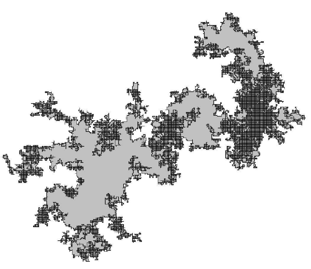
Let us make precise what we mean by area enclosed by a Brownian loop. Let $B$ denote a Brownian bridge in ${\mathbb{C}}$ of time duration 1. I.e. the law of $B_{t},\,0\leq t\leq 1$ is the same as the law of $W_{t}-tW_{1},\,0\leq t\leq 1$, where $W$ is just a standard Brownian motion in ${\mathbb{C}}$. ${\mathbb{C}}\setminus B[0,1]$, i.e. the complement of the path, has a unique infinite connected component $H$. The hull $T$ generated by the Brownian loop is by definition ${\mathbb{C}}\setminus H$. Let $\cal{A}$ be the random variable whose value is the area of $T$. In this paper, we will prove

We would like to explain now how this result is related to the problem of windings of a Brownian loop. In [16], Yor gave an explicit formula for the law of the index of a Brownian loop around a fixed point $z$. A point with a non-zero index has to be inside the loop. Using this fact, it is almost possible to describe the probability that a point is inside the loop, modulo the problem of the zero index; indeed, there are some regions inside the Brownian loop which are of index zero. It seems hard to control the influence of these zero-index points inside the curve. In the last section, using our main result, theorem 1.1, combined with the law of the index given by Yor, we find that the expected area of the set of points inside the loop that have index zero is $\frac{\pi}{30}$. We also compute the expected areas of the regions of index $n\in{\mathbb{Z}}\setminus\{0\}$.

In [2], using physics methods, Contet, Desbois and Ouvry obtained the values of the expected areas for the non-zero regions. In their paper, they noted the different nature of the $n=0$ sector (the points in the plane of zero index) and emphasized that “it would be interesting to distinguish in the $n=0$ sector, curves which do not enclose the origin from curves which do enclose the origin but an equal number of times clockwise and anticlockwise”. Their values in the case $n\neq 0$ agree with our results; they argue that the 0-case cannot be treated within the scope of their analysis.

From a probabilistic viewpoint, it also appears that usual techniques for Brownian motion are not strong enough to obtain the expected area of the Brownian loop or the expected area of the 0-index region inside the Brownian loop. However, the computation of the expected area of the $n$-index region for $n\neq 0$ was within reach using the result of Yor. To our knowledge this computation had not been carried out in a mathematical way before.

Let us briefly explain why usual techniques for Brownian motion seem unable to tackle the problem of the expected area of the Brownian loop. Basically, the enclosed area depends only on the boundary of the hull generated by the Brownian loop. The frontier of the Brownian loop concerns only a small subset of the time duration $[0,1]$. In some sense, on certain time-intervals, the enclosed area does not depend much on the behavior of the Brownian motion. So, this problem needs a good description of the frontier of a Brownian loop. Recently, Lawler, Schramm and Werner proved a conjecture of Mandelbrot that the Hausdorff dimension of the Brownian frontier is $4/3$. For this purpose they used the value of intersection exponents computed with the help of $SLE$ curves, see for instance [6] and references therein. The description of the Brownian frontier via $SLE$ can be done in a slightly different way using the conformal-restriction point of view, see [5]. We will use this approach, and so will present to the reader the facts needed about conformal restriction measures in the next section.

The paper gives another striking example of a simple result concerning planar Brownian motion that seemed out of reach using the usual stochastic calculus approach, but that can be derived using conformal invariance and $SLE$. For a thorough account on $SLE$ processes, see [3, 13].

Conformal restriction measures in ${\mathbb{H}}$ are measures supported on the set of closed subsets $K$ of ${\mathbb{H}}$ such that $\overline{K}\cap{\mathbb{R}}=\{0\}$, $K$ is unbounded and ${\mathbb{H}}\setminus K$ has two infinite connected components, that satisfy the conformal restriction property : for all simply connected domains $H\subset{\mathbb{H}}$ such that ${\mathbb{H}}\setminus H$ is bounded and bounded away from the origin, the law of $K$ conditioned on $K\subset H$ is the law of $\Phi(K)$, where $\Phi$ is any conformal transformation from $H$ to ${\mathbb{H}}$ preserving $0$ and $\infty$ (this law doesn’t depend of the choice of $\Phi$). It is proved in [5] that there is only one real parameter family of such restriction measures, ${\bf P}_{\alpha}$ where $\alpha\geq 5/8$. These measures are uniquely described by the following property : for all closed $A$ in ${\mathbb{H}}$ bounded and bounded away from $0$,

where $\Phi_{A}$ is a conformal transformation from ${\mathbb{H}}\setminus A$ into ${\mathbb{H}}$ such that $\Phi_{A}(z)/z\rightarrow 1$, when $z\rightarrow\infty$. To aid with the notation for the rest of the paper whenever we write $\Phi_{A}$ we will be assuming that we have chosen the translate with the additional property $\Phi_{A}(0)=0$. ${\bf P}_{5/8}$ is the law of chordal $SLE_{8/3}$, and ${\bf P}_{1}$ can be constructed by filling the closed loops of a Brownian excursion in ${\mathbb{H}}$ (Brownian motion started at $0$ conditioned to stay in ${\mathbb{H}}$). An important property of these conformal restriction measures is that using two independent restriction measures ${\bf P}_{\alpha_{1}}$ and ${\bf P}_{\alpha_{2}}$, we can construct ${\bf P}_{\alpha_{1}+\alpha_{2}}$ by filling the “inside” of the union of $K_{1}$ and $K_{2}$. This “additivity” property and the construction of ${\bf P}_{5/8}$ and ${\bf P}_{1}$ give the good description of the Brownian motion in terms of $SLE$ curves, namely, 8 $SLE_{8/3}$ give the same hull as 5 Brownian excursions.

Since, we want to describe the boundary of loops of time duration 1, we will first create loops with the use of the infinite hulls described above. Restriction measures are conformally invariant (Brownian excursion, $SLE_{8/3}$,..), so we had better use conformal maps. There is obviously no conformal map which sends both $\infty$ and 0 to 0, so the natural idea is to consider a Möbius transformation preserving ${\mathbb{H}}$ which maps 0 to 0, and $\infty$ to $\varepsilon$. We can choose

The limit when $\varepsilon$ goes to zero of the measures $\text{m}_{\varepsilon}({\bf P}_{1})$ is the dirac measure at $\{0\}$. The good renormalization to keep something interesting is in $\varepsilon^{2}$. Hence, we define the Brownian bubble measure in ${\mathbb{H}}$ as :

This measure was introduced in [5], and it is an important tool for studying the link between $SLE$ curves and the Brownian loop soup (see [4]). It was already noted in [5, 7], as an easy consequence of the “additivity” property described above, that

The last measure can be seen as an infinite measure on “$SLE_{8/3}$ loops”, let us call this measure $\mu^{\text{sle}}$. Recall, that we are interested in a Brownian loop of time duration 1. We have the following time decomposition for $\mu^{\text{bub}}$, (see [4],[3])

where ${\bf P}_{t}^{\text{br}}$ is the law of a one-dimensional Brownian bridge of time duration $t$, and ${\bf P}_{t}^{\text{exc}}$ is the law of an Itô Brownian excursion re-normalized to have time $t$. ${\bf P}_{t}^{\text{br}}\times\,{\bf P}_{t}^{\text{exc}}$ is the law of an ${\mathbb{H}}$-Brownian bridge of time duration $t$, by considering the one dimensional bridge as the $x$ coordinate of the curve, and the excursion as the $y$ coordinate. Unfortunately, it is hard to compute fixed-time quantities with $SLE$ techniques. Thus, we will compute a “geometric quantity” using $SLE_{8/3}$, and then extract ${\bf E}(\mathcal{A})$ from this geometric value by using the relation $\mu^{\text{bub}}=8/5\mu^{\text{sle}}$ and the decomposition  2.2.

Let us explain in a few words why we need to deal with Brownian bridges in ${\mathbb{H}}$ and cannot work directly with bridges in ${\mathbb{C}}$. The underlying idea is the fact that one needs to choose a starting point on the boundary of the Brownian loop for the $SLE$ loop representation. A natural choice is the (almost surely) unique lower point, this is why we are interested in ${\mathbb{H}}$ quantities. So let $\mathcal{A}^{\mathbb{H}}$ be the random variable giving the area of an ${\mathbb{H}}-$Brownian bridge of time duration one. Working with $\mathcal{A}^{\mathbb{H}}$ will turn out not to be a problem since, as the reader might already suspect, the random variables $\mathcal{A}$ and $\mathcal{A}^{\mathbb{H}}$ have the same law.

For the geometric quantity, we could choose to compute $\int A(\gamma)d\mu^{\text{sle}}$, where $A(\gamma)$ is the area enclosed in ${\mathbb{H}}$ by the “curve” $\gamma$, but this integral is infinite. Let $\gamma^{*}$ be the radius of the curve $\gamma$, that is, $\gamma^{*}=\sup_{0\leq t\leq t_{\gamma}}|\gamma(t)|$. We may consider the “expected” area under the law $\mu^{\text{sle}}$ “conditioned” on $\gamma^{*}=1$. Here, $\mu^{\text{sle}}$ is not a probability measure so the term “expected value” is not correct, and the conditioning is on a set of $\mu^{\text{sle}}-$measure equal to 0. But we have the following rigorous definition :

Using $\mu^{\text{sle}}=5/8\mu^{\text{bub}}$, we can write in the same way :

Thus, $\mu^{\text{sle}}(A|\gamma^{*}=1)$ represents at the same time the “expected” area of an $SLE_{8/3}$ loop conditioned to touch the half circle of radius one and the expected area of a Brownian bubble with the same conditioning. With the use of the restriction property for $SLE_{8/3}$, we will be able to compute in the last section $\mu^{\text{sle}}(A|\gamma^{*}=1)$. Before, in the coming section, we will find the relationship between ${\bf E}(\mathcal{A})$ and $\mu^{\text{sle}}(A|\gamma^{*}=1)$.

In this section we will prove the following

In this section we prove lemma 4.1, the proof provides a good example of the use of standard techniques for $SLE_{8/3}$. We have chosen to leave out some algebraic details in order to allow the reader to focus on the main ideas.

Note that theorem 1.1 follows immediately from this lemma and lemma 3.1.

Below we state a result that we have used extensively in our proof; for the reader’s sake we will sketch a proof. This lemma gives an equivalent expression to the one given by Schramm, in [10].

Remark : We would like to point out that the 1/5 in the final result, comes from the 8/5 in the restriction formula 2.1.

Let $z\in{\mathbb{C}}\setminus\{0\}$ be fixed, and $(B_{t})_{0\leq t\leq 1}$ a Brownian loop in ${\mathbb{C}}$ starting at 0. Almost surely $z\not\in\{B_{s}:0\leq s\leq 1\}$, and therefore we can define its index $n_{z}$. More precisely, $\forall s\in[0,1],B_{s}-z=R_{s}^{z}\exp(i\theta_{s}^{z})$, where $R_{s}^{z}=|B_{s}-z|$ and $\theta_{s}^{z}$ is any continuous representative of the argument. The index $n_{z}$ is by definition $\frac{\theta_{1}^{z}-\theta_{0}^{z}}{2\pi}$ ; this is the number of times that the Brownian particle winds around $z$. For each $n\in{\mathbb{Z}}$, $n\neq 0$, let $\mathcal{W}_{n}$ denote the area of the open set of points of index $n_{z}=n$. This random variable can be written as :

Let $\mathcal{W}_{0}$ be the area of the open set of points inside the loop that have index zero :

Since the Brownian curve is of Lebesgue measure zero, we have the following decomposition of the area $\mathcal{A}$ inside the Brownian loop (basically, the Brownian path does not take much place inside its hull)

Hence :

Using results of Yor [16], it will be straightforward to compute ${\bf E}(\mathcal{W}_{n})$ for $n\neq 0$. And, hence, by subtracting from $\pi/5$, one can obtain the value of ${\bf E}(\mathcal{W}_{0})$.

Remark : This result is consistent with the asymptotic result obtained by Werner in [12], about the area $A_{n}^{t}$ of the set of points around which the planar Brownian motion (not the loop) winds around $n$ times on $[0,t]$. It is indeed proved that $A_{n}^{t}$ is equivalent (in the $L^{2}$-sense) to $\frac{t}{2\pi n^{2}}$ as $n$ goes to infinity. Very roughly the area of the $n$-sector for large $n$ comes from local contributions along the path, hence the global picture of the hull is not relevant; that is why, both Brownian motion and Brownian bridge should have the same asymptotics. Werner’s proof requires to compute the asymptotics of the first and second moments. This present paper gives exact computations for the first moments in the case of the loop, but it does not provide any information about the second moments.

References

- [1] John Cardy, Mean area of self-avoiding loops, Phys. Rev. Letters 72 (1994), 1580–1583.
- [2] A. Comtet, J. Desbois, S. Ouvry, Winding of planar Brownian curves, J. Phys. A: Math. Gen. 23 (1990) 3563-3572.
- [3] Gregory F. Lawler, Conformally Invariant Processes in the Plane, AMS (2005).
- [4] Gregory F. Lawler and Wendelin Werner, The Brownian loop soup, Probab. Theory Related Fields 128 (2004), 565–588.
- [5] Gregory F. Lawler, Oded Schramm and Wendelin Werner, Conformal restriction. The chordal case, J. Amer. Math. Soc. 16 (2003), 917–955.
- [6] Gregory F. Lawler, Oded Schramm and Wendelin Werner, The dimension of the planar Brownian frontier is 4/3, Math. Res. Lett. 8 (2001), 401–411.
- [7] Gregory F. Lawler, Oded Schramm and Wendelin Werner, On the scaling limit of planar self-avoiding walk, to appear in Fractal geometry and applications, A jubilee of Benoit Mandelbrot, AMS Proc. Symp. Pure Math.
- [8] Christoph Richard, Area distribution of the planar random loop boundary, J. Phys. A. 37 (2004), 4493–4500.
- [9] John Thacker, Hausdorff Dimension of the Brownian Loop Soup, in preparation (2005).
- [10] Oded Schramm, A percolation formula, Electron. J. Probab. vol. 7, paper no. 2 (2001), 1–13.
- [11] Wim Vervaat, A relation between Brownian bridge and Brownian excursion, Ann. Probab. 7 (1979), 143–149.
- [12] Wendelin Werner, Sur l’ensemble des points autour desquels le mouvement brownien plan tourne beaucoup, Probability Theory and Related Fields, 99 (1994), 111-142.
- [13] Wendelin Werner, Random planar curves and Schramm-Loewner evolutions, Lecture notes from the 2002 Saint-Flour summer school, Springer, L.N. Math. 1840 (2004), 107–195.
- [14] Wendelin Werner, Conformal restriction and related questions, 2003, math.PR/0307353.
- [15] Wendelin Werner, SLEs as boundaries of clusters of Brownian loops, C. R. Acad. Sci. Paris Ser. I Math. 337 (2003), 481–486.
- [16] Marc Yor, Loi de l’indice du lacet brownien, et distribution de Hartman-Watson , Z. Wahrsch. Verw. Gebiete 53 (1980), 71–95.