Fermionic characters and arbitrary highest-weight integrable $\widehat{{\mathfrak{sl}}}_{r+1}$ -modules

Eddy Ardonne, Rinat Kedem, Michael Stone Address: EA: Department of Physics, University of Illinois, 1110 W. Green St., Urbana, IL 61801. ardonne@uiuc.edu Address: RK: Department of Mathematics, University of Illinois, 1409 W. Green Street, Urbana, IL 61801. rinat@uiuc.edu Address: MS: Department of Physics, University of Illinois, 1110 W. Green St., Urbana, IL 61801. m-stone5@uiuc.edu

Date: August 11, 2026

Abstract.

This paper contains the generalization of the Feigin-Stoyanovsky construction to all integrable $\widehat{{\mathfrak{sl}}}_{r+1}$ -modules. We give formulas for the $q$ -characters of any highest-weight integrable module of $\widehat{{\mathfrak{sl}}}_{r+1}$ as a linear combination of the fermionic $q$ -characters of the fusion products of a special set of integrable modules. The coefficients in the sum are the entries of the inverse matrix of generalized Kostka polynomials in $q^{-1}$ . We prove the conjecture of Feigin and Loktev regarding the $q$ -multiplicities of irreducible modules in the graded tensor product of rectangular highest weight-modules in the case of ${\mathfrak{sl}}_{r+1}$ . We also give the fermionic formulas for the $q$ -characters of the (non-level-restricted) fusion products of rectangular highest-weight integrable $\widehat{{\mathfrak{sl}}}_{r+1}$ -modules.

1. Introduction

Fermionic formulæ for characters of highest-weight modules of affine algebras or vertex algebras first appeared in a purely algebraic context [17]. They were later shown [13, 12] to be related to the partition functions of certain statistical mechanical systems at their critical points. These character formulæ have desirable combinatorial properties, such as the manifest positivity of the coefficients that represent weight-space multiplicities. They also have a physical significance because they reflect the quasi-particle content of the statistical mechanical system. Consequently, algebraic constructions of bases for representations which reveal this combinatorial structure are important, and have been studied using several methods in the past dozen years.

One such method is that of Feigin and Stoyanovskiĭ [23]. These authors used a theorem of Primc [21] to give an interesting construction of the vacuum integrable modules of the affine algebra $\widehat{{\mathfrak{g}}}$ associated to any simple Lie algebra ${\mathfrak{g}}$ . Their construction relies on the loop generators of the affine algebra. Physical systems associated with such integrable $\widehat{{\mathfrak{g}}}$ -modules are generalizations of the Heisenberg spin chain in statistical mechanics, or the WZW model in conformal field theory.

The formulæ of Feigin-Stoyanovskiĭ [23] have an attractive interpretation in terms of (a bosonic version of) non-abelian quantum Hall states [19, 2]. In these states there are $r$ “types” of particles that obey a generalized exclusion principle: the wave function vanishes if any $k+1$ particles occupy the same state. Here $r$ is the rank of the algebra and $k$ is the level of the integrable $\widehat{{\mathfrak{g}}}$ -module. In the presence of quasi-particle excitations, the wave functions can also vanish if fewer than $k+1$ particles occupy the same state. The statistics of the quasi-particles is ‘dual’ to the statistics of the fundamental particles [1].

The original construction of Feigin-Stoyanovskiĭ can be used to compute [23] characters of vacuum (with highest weight $k\Lambda_{0}$ ) representations of affine algebras. Later, Georgiev [10, 9] generalized it to some modules in the ADE series, with particularly simple highest weights, of the form $l\omega_{j}+k\Lambda_{0}$ , corresponding to special rectangular Young diagrams. (Here $\omega_{j}$ are certain fundamental ${\mathfrak{g}}$ -weights, and $l\in{\mathbb{Z}}_{\geq 0}$ .)

In general, no fermionic formulæ are available for arbitrary highest-weight, integrable $\widehat{{\mathfrak{g}}}$ -modules. In this paper, we resolve this problem for the case of ${\mathfrak{sl}}_{r+1}$ .

We explain, in terms of the functional realization of Feigin and Stoyanovskĭ, why such ‘rectangular highest weight’ modules are very special, and why there is no direct fermionic construction for other modules. However, we prove that it is possible to compute the character of any module as a finite sum of fermionic characters of the ‘rectangular’ highest-weight modules. The coefficients in this sum are the entries of the inverse matrix of generalized Kostka polynomials. These coefficients are, however, not manifestly positive (or even of positive degree).

In our construction we are naturally led to the graded tensor product of Feigin and Loktev [8] of finite-dimensional ${\mathfrak{g}}$ -modules. In the case of irreducible ${\mathfrak{sl}}_{r+1}$ -modules with highest weights of the form $l\omega_{j}$ (where $\omega_{j}$ is any fundamental weight), we compute the explicit fermionic form of the graded multiplicities of irreducible modules in the the Feigin-Loktev tensor product, thus proving two of the conjectures of [8]: That the graded tensor product in this case is independent of the evaluation parameters, and that it is related to the generalized Kostka polynomials of [22, 16].

The plan of the paper is as follows. In Section 2 we give the basic definitions of the algebra and its modules. In Sections 3 and 4, we supply the details of the generalized construction of [23] for integrable modules of $\widehat{{\mathfrak{sl}}}_{r+1}$ , with highest weights corresponding to rectangular Young diagrams. In Section 5, we explain a similar calculation of graded characters of conformal blocks or coinvariants (the fusion product of [8]), which turn out to be related to the generalized Kostka polynomials of [22, 16]. We then use this calculation in Section 6 to compute the characters of arbitrary highest-weight representations. See theorem 6.3 for the main result.

Although, for the sake of clarity, we concentrate in this paper on the case of $\widehat{\mathfrak{g}}=\widehat{\mathfrak{sl}}_{r+1}$ , the generalization to affine algebras associated with other simple Lie algebras is possible, but in that case one should replace the notion of integrable $\widehat{{\mathfrak{g}}}$ -modules with irreducible ${\mathfrak{g}}$ -modules as their top component with those which have (the degeneration to the classical case of) Kirillov-Reshetikhin modules as their top component. We will give this construction in a future publication.

Acknowledgements: The work of E.A. is supported by NSF grants numbers DMR-04-42537 and DMR-01-32990; that of M.S. by NSF grant DMR-01-32990. R.K. would like to thank B. Feigin and S. Loktev for many useful discussions.

2. Notation

2.1. Current generators of affine algebras

Let ${\mathfrak{g}}={\mathfrak{sl}}_{r+1}$ and let $\Pi=\{\alpha_{i}\ |\ i=1,\ldots,r\}$ denote its simple roots, and $\{\omega_{i}\ |\ i=1,\ldots,r\}$ the fundamental weights. Let $\{e_{\alpha_{i}}=e_{i}\ |\ i=1,\ldots,r\}$ denote the corresponding generators of ${\mathfrak{n}}_{+}$ , and $\{f_{\alpha_{i}}=f_{i}\ |\ i=1,\ldots,r\}$ those of ${\mathfrak{n}}_{-}$ . We have the Cartan decomposition ${\mathfrak{sl}}_{r+1}\simeq{\mathfrak{n}}_{+}\oplus{\mathfrak{h}}\oplus{\mathfrak{n}}_{-}$ , where ${\mathfrak{h}}$ is the Cartan subalgebra.

Irreducible, finite-dimensional highest-weight ${\mathfrak{g}}$ -modules $\pi_{\lambda}$ are parametrized by weights $\lambda\in P^{+}$ , that is, $\lambda=l_{1}\omega_{1}+\cdots+l_{r}\omega_{r}$ with $l_{i}\in{\mathbb{Z}}_{\geq 0}$ . The subset of $P^{+}$ consisting of weights $\lambda$ such that $\sum_{i=1}^{r}l_{i}\leq k$ is called the set of level- $k$ restricted weights, $P^{+}_{k}$ .

The affine Lie algebra associated with ${\mathfrak{g}}$ is $\widehat{{\mathfrak{g}}}$ , where

\widehat{{\mathfrak{g}}}\simeq{\mathfrak{g}}\otimes{\mathbb{C}}[t,t^{-1}]\oplus{\mathbb{C}}c\oplus{\mathbb{C}}d,

where $c$ is central and

(2.1)

[d,x\otimes t^{n}]=-nx\otimes t^{n}\ .

We denote the current generators by $x[n]\overset{\rm def}{=}x\otimes t^{n}$ , $x\in{\mathfrak{sl}}_{r+1}$ . Let $\langle x,y\rangle$ be the symmetric bilinear form on ${{\mathfrak{sl}}_{r+1}}$ . Then the relations between the currents are

[x\otimes f(t),y\otimes g(t)]_{\widehat{{\mathfrak{g}}}}=[x,y]_{{\mathfrak{g}}}f(t)g(t)+c\ \langle x,y\rangle\oint_{t=0}f^{\prime}(t)g(t)dt,

where $[\cdot,\cdot]_{{\mathfrak{g}}}$ is the corresponding commutator in ${\mathfrak{g}}$ .

The Cartan decomposition is $\widehat{{\mathfrak{g}}}\simeq\widehat{{\mathfrak{n}}}_{+}\oplus\widehat{{\mathfrak{h}}}\oplus\widehat{{\mathfrak{n}}}_{-}$ with $\widehat{{\mathfrak{n}}}_{\pm}={\mathfrak{n}}_{\pm}\oplus({\mathfrak{sl}}_{r+1}\otimes t^{\pm 1}{\mathbb{C}}[t^{\pm 1}])$ and $\widehat{{\mathfrak{h}}}={\mathfrak{h}}\oplus{\mathbb{C}}c\oplus{\mathbb{C}}d$ . The algebra $\widehat{{\mathfrak{g}}}^{\prime}$ is the algebra obtained by dropping the generator $d$ .

We will frequently use generating functions for current generators of the affine algebra, which we define by

(2.2)

x(z)=\sum_{n\in{\mathbb{Z}}}x[n]z^{-n-1},\ x\in{\mathfrak{sl}}_{r+1}.

Note that the convention for the current generators in (2.2) is different from that used by [23, 4].

2.2. Affine algebra modules

On any irreducible $\widehat{{\mathfrak{sl}}}_{r+1}$ -module, $c$ acts by a constant $k$ called the level of the representation. A cyclic highest-weight ${\widehat{{\mathfrak{g}}}}$ -module with highest weight $\Lambda=\lambda+k\Lambda_{0}+m\delta$ is a cyclic module generated by the action of ${\widehat{{\mathfrak{g}}}}$ on a highest-weight vector $v_{\lambda}$ , such that

(2.3)		$\displaystyle\widehat{{\mathfrak{n}}}_{+}v_{\lambda}=0,$
(2.4)		$\displaystyle hv_{\lambda}=\lambda(h)v_{\lambda},\ {\rm for}\ h\in{\mathfrak{h}}\subset{\mathfrak{g}},\quad cv_{\lambda}=kv_{\lambda},\quad dv_{\lambda}=mv_{\lambda}.$

The universal such module is the Verma module $M(\Lambda)\simeq U(\widehat{{\mathfrak{n}}}_{-})$ . If $k\in{\mathbb{N}}$ and $\lambda\in P_{k}^{+}$ , the quotient of the Verma module by its maximal submodule is an irreducible, highest-weight integrable ${\widehat{{\mathfrak{g}}}}$ -module, which we denote by $V_{\lambda}$ (we assume $k$ is fixed in this notation). The structure of the cyclic module generated by a highest-weight vector $v_{\lambda}$ is independent of $m$ , so it is generally convenient to set $m=0$ .

Definition 2.1.

Let $M$ be an irreducible cyclic highest-weight module with highest weight $\Lambda=\lambda+k\Lambda_{0}$ , generated by the highest-weight vector $v_{\lambda}$ . The subspace generated by the action of the subalgebra ${\mathfrak{g}}\otimes 1\simeq{\mathfrak{g}}$ on $v_{\lambda}$ is called the top component of $M$ . It is isomorphic as a ${\mathfrak{g}}$ -module to $\pi_{\lambda}$ .

The irreducible, finite-dimensional ${\mathfrak{g}}$ -module $\pi_{\lambda}$ is characterized as the quotient of the Verma module of ${\mathfrak{g}}$ by the left ideal in ${\mathfrak{g}}$ generated by $f_{i}^{l_{i}+1}$ . Similarly, the integrable module $V_{\lambda}$ is the quotient of the Verma module $M(\Lambda)$ of $\widehat{{\mathfrak{g}}}$ by the left ideal in ${\widehat{{\mathfrak{g}}}}$ generated by $f_{i}[0]^{l_{i}+1}$ , plus one additional generator, $e_{\theta}[-1]^{k-\theta(\lambda)+1}$ where $\theta=\alpha_{1}+\cdots+\alpha_{r}$ .

A characterization of the maximal proper submodule $M^{\prime}(\Lambda)$ of $M(\Lambda)$ in the case of integrable modules was given in [21] in terms of the algebra of current generators.

Note that on any highest-weight module, the current (2.2) acts as a Laurent series in $z$ . Therefore, products of currents make sense when acting on a highest-weight module, and one can consider the associative algebra of currents. Formally, the coefficients of $z^{n}$ in products of currents of the form $x(z)y(z)$ exist only in a completion $\overline{U}$ of $U(\widehat{{\mathfrak{g}}})$ .

Theorem 2.2.

[21] Let $M(\Lambda)$ be a Verma module with highest weight $\Lambda=\lambda+k\Lambda_{0}$ , with $\lambda\in P^{+}_{k}$ and $k\in{\mathbb{N}}$ . Denote its maximal proper submodule by $M^{\prime}(\Lambda)$ , such that $V_{\lambda}\simeq M(\Lambda)/M^{\prime}(\Lambda)$ . Let $R$ be the subspace in $\overline{U}$ generated by the adjoint action of $U({\mathfrak{sl}}_{r+1})$ on the coefficients of $e_{\theta}(z)^{k+1}$ . Then $M^{\prime}(\Lambda)=RM(\Lambda)$ .

Again, the elements in $R$ act as well-defined elements of $U(\widehat{{\mathfrak{g}}})$ on $M(\Lambda)$ . We call the set of currents which result from the adjoint action of ${\mathfrak{sl}}_{r+1}$ on the current $e_{\theta}(z)^{k+1}$ the integrability conditions. For example, for any root $\alpha$ , the coefficients of $e_{\alpha}(z)^{k+1}$ are in $R$ .

3. The semi-infinite construction of Feigin and Stoyanovskiĭ

Theorem 2.2 was used by Feigin and Stoyanovskiĭ [23] to give a construction of the integrable modules in the case where $\Lambda=k\Lambda_{0}$ . The construction naturally gives rise to fermionic formulæ for the characters of integrable modules. We will explain the details of the construction of [23] below.

3.1. Principal subspaces

For arbitrary integrable highest weight $\Lambda=\lambda+k\Lambda_{0}$ , let $v_{\lambda}$ be the highest-weight vector of $V_{\lambda}$ . Consider the subalgebra

\widetilde{{\mathfrak{n}}}_{-}\overset{\rm def}{=}{\mathfrak{n}}_{-}\otimes{\mathbb{C}}[t,t^{-1}]

acting on $v_{\lambda}$ .

Definition 3.1.

Define the principal subspace $W_{\lambda}=W_{\lambda}^{(0)}=U({\widetilde{{\mathfrak{n}}}_{-}})v_{\lambda}\subset V_{\lambda}$ . Similarly, define the principal subspaces $W_{\lambda}^{(N)}=U({\widetilde{{\mathfrak{n}}}_{-}})T_{N}v_{\lambda}$ , where where $T_{N}=t_{\alpha(N)}$ is the affine Weyl translation corresponding to the root $\alpha(N)=\sum_{i}N_{i}\alpha_{i}$ (in the notation of [11] (6.5.2)), where $N_{i}$ are positive integers such that $(C_{r}{\mathbf{N}})_{\alpha}=2N$ for all ${\alpha}$ , and $C_{r}$ is the Cartan matrix of ${\mathfrak{sl}}_{r+1}$ .

Lemma 3.2.

This choice of $\alpha(N)$ gives a sequence of inclusions

(3.1)

W_{\lambda}^{(0)}\subset W_{\lambda}^{(1)}\subset\cdots\subset W_{\lambda}^{(N)}\subset\cdots,

such that the inductive limit of the sequence (3.1) as $N\to\infty$ is the integrable module $V_{\lambda}$ .

The inclusions follow from the fact that $v_{\lambda}\in W^{(N)}_{\lambda}$ . The fact that the inductive limit indeed gives the full module is not obvious (see [20, 5]) but follows from the fact that the module is integrable.

In fact, this Theorem was proven in [23] for the following cases: $\widehat{{\mathfrak{sl}}}_{2}$ for arbitrary highest weight, and $\widehat{{\mathfrak{sl}}}_{3}$ with $\Lambda=k\Lambda_{0}$ . This was done by computing the characters in the limit $N\to\infty$ , and comparing them with the known character formulæ for $V_{\lambda}$ of [17].

In [10, 9], certain combinatorial proofs were provided using ideas related to those of [23] (with differently defined principal subspaces) for rectangular highest weights, for all simply laced algebras. The principal subspaces of that paper are different from those used here, as [10] uses what amounts to a different subalgebra to generate the subspace.

In this paper, we will continue this program by giving the character formulæ for arbitrary highest-weight modules of ${\mathfrak{sl}}_{r+1}$ . It turns out that the methods of [23] are not sufficient for the case of non-rectangular representations, and instead we must resort to computing the characters of certain fusion products of representations, and decomposing them in terms of irreducible modules. The result is a formula which is a sum of fermionic formulas of the form found in [23, 10, 9], where the coefficients in the sum are elements of ${\mathbb{Z}}[q^{-1}]$ .

3.2. Relations in the principal subspace

Let us characterize the ideal $I_{\lambda}$ , where $W_{\lambda}\simeq U({\widetilde{{\mathfrak{n}}}_{-}})/I_{\lambda}$ . Using a PBW-type argument, it is easy to see that $W_{\lambda}=U({\mathfrak{n}}_{-}\otimes{\mathbb{C}}[t^{-1}])v_{\lambda}$ , because the highest-weight vector $v_{\lambda}$ is annihilated by ${\mathfrak{n}}_{-}\otimes t{\mathbb{C}}[t]$ . Thus, $I_{\lambda}$ includes the left ideal generated by $\{f_{\alpha}[n]\ |\ n>0,\alpha\in\Pi\}$ .

The ideal contains the two-sided ideal generated by relations in the Lie algebra. In terms of generating functions, these relations are

	$\displaystyle[f_{\alpha_{i}}(z),f_{\alpha_{j}}(w)]$	$\displaystyle=$	$\displaystyle\left\{\begin{array}[]{ll}0,&\|i-j\|\neq 1\\ w^{-1}\delta(w/z)f_{\alpha_{i}+\alpha_{j}}(z),&\|i-j\|=1\end{array}\right.$
(3.5)		$\displaystyle\left[f_{\alpha_{i}}(z),{[f_{\alpha_{i}}(w),f_{\alpha_{i\pm 1}}(u)]}\right]$	$\displaystyle=$	$\displaystyle 0,$

where $\delta(z)=\sum_{n\in{\mathbb{Z}}}z^{n}$ . These two relations together mean that matrix elements involving the product $f_{i}(z)f_{{i\pm 1}}(w)$ have a simple pole whenever $z=w$ , and that the residue of this pole commutes with $f_{i}(u)$ .

The integrability condition

(3.6)

f_{i}(z)^{k+1}v=0,\quad v\in V_{\lambda},\ 1\leq i\leq r,

for any implies that $I_{\lambda}$ contains the two-sided ideal generated by the coefficients of $z^{n}$ of $f_{i}(z)^{k+1}$ (in the appropriate completion of the universal enveloping algebra).

Finally there are the relations which follow from the integrability of the top component $\pi_{\lambda}$ of $V_{\lambda}$ , which is a subspace of $W_{\lambda}$ also. Therefore, $I_{\lambda}$ contains the left ideal generated by $f_{i}[0]^{l_{i}+1}$ . The integrability condition involving $e_{\theta}[-1]$ does not play a role, because it is not an element of $U({\widetilde{{\mathfrak{n}}}_{-}})$ .

3.3. Construction of the dual space

In order to compute the characters of the principal subspace $W_{\lambda}$ , we describe its dual space. This will enable us to calculate the character for sufficiently simple $\lambda$ . The dual space is spanned by the coefficients of monomials of the form $x_{1}^{n_{1}}\cdots x_{m}^{n_{m}}$ of matrix elements in the set

\mathcal{F}_{\lambda}=\left\{\langle w|f_{{i_{1}}}(x_{1})\cdots f_{{i_{m}}}(x_{m})|v_{\lambda}\rangle\ |\ \quad w\in V_{\lambda}^{*},\ m\geq 0,\ 1\leq i_{a}\leq r\right\},

where $V^{*}_{\lambda}$ is the restricted dual module. Given an ordering of the generators, the function above is defined in the region $|x_{i}|>|x_{i+1}|$ , and therefore the coefficient of $x_{1}^{n_{1}}\cdots x_{m}^{n_{m}}$ for given integers $n_{j}$ is given by the expansion in this regime. Below, we shall refer to the function space $\mathcal{F}_{\lambda}$ itself as the dual space, and specify an appropriate pairing. This space can be characterized by its pole structure and vanishing conditions.

3.3.1. The dual space to $U({\widetilde{{\mathfrak{n}}}_{-}})$

Let us first consider the larger function space $\mathcal{G}$ , dual to the universal enveloping algebra $U=U({\widetilde{{\mathfrak{n}}}_{-}})$ . The algebra $U$ is spanned by words in the letters $\{f_{\alpha_{i}}[n]\ |\ i=1,\ldots,r,\ n\in{\mathbb{Z}}\}$ , and it is ${\mathfrak{h}}$ and $d$ -graded. The graded component $U[\mathbf{m}]_{d}$ , where ${\mathbf{m}}=(m^{(1)},\ldots,m^{(r)})^{T}$ , is spanned by the elements $f_{i_{1}}[n_{1}]\cdots f_{i_{m}}[n_{m}]$ , of ${\mathfrak{h}}$ -weight $\sum_{\alpha}m^{(\alpha)}\alpha=\sum_{j}\alpha_{i_{j}}$ and $-\sum_{i}n_{i}=d$ .

The dual space to $U$ is also ${\mathfrak{h}}$ - and $d$ -graded. Denote by $U[{\mathbf{m}}]$ the ${\mathfrak{h}}$ -graded component, and by ${\mathcal{G}}[\mathbf{m}]$ the dual to it. This is a space of functions in the variables

\mathbf{x}=\{x_{i}^{(\alpha)}\ |\ i=1,\ldots,m^{(\alpha)},\alpha=1,\ldots,r\},

where $x_{i}^{(\alpha)}$ is the variable corresponding to a generator of the form $f_{\alpha}(x_{i}^{(\alpha)})$ . We define the pairing $(\cdot,\cdot)$ between $U$ and $\mathcal{G}$ inductively, as follows:

	$\displaystyle(1,1)=1$
(3.7)		$\displaystyle(g(\mathbf{x}),Mf_{\alpha}[n])=\left(\frac{1}{2\pi i}\oint_{x^{(\alpha)}_{1}=0}(x_{1}^{(\alpha)})^{n}g(\mathbf{x})dx_{1}^{(\alpha)},M\right),\quad M\in U,$

where the contour of integration is taken counter-clockwise around the point $x^{(\alpha)}_{1}=0$ , in such a way that all other points are excluded, $|x_{1}^{(\alpha)}|<|x_{j}^{(\alpha^{\prime})}|$ . Similarly,

\displaystyle(g(\mathbf{x}),f_{\alpha}[n]M)=\left(\frac{1}{2\pi i}\oint_{x^{(\alpha)}_{1}=0}(x_{1}^{(\alpha)})^{n}g(\mathbf{x})dx_{1}^{(\alpha)},M\right),

the contour is taken clockwise.

The commutation relations between the currents are equivalent to the operator product expansion (OPE)

f_{i}(z)f_{i\pm 1}(w)=\frac{f_{\alpha_{i}+\alpha_{i\pm 1}}(w)}{z-w}+\hbox{regular terms}

where “regular terms” refers to terms which have no pole at $z=w$ , and the expansion of the denominator is taken in the region $|z|>|w|$ . Due to the OPE’s, it is clear that functions in $\mathcal{G}[\mathbf{m}]$ will have at most a simple pole whenever $x_{j}^{(\alpha)}=x_{k}^{(\alpha\pm 1)}$ . Thus, functions in $\mathcal{G}[\mathbf{m}]$ are rational functions of the form

(3.8)

g(\mathbf{x})=\frac{g_{1}(\mathbf{x})}{\prod_{i,j,\alpha}(x_{i}^{(\alpha)}-x_{j}^{(\alpha+1)})},

where $g_{1}(\mathbf{x})$ are polynomials in $(x_{i}^{(\alpha)})^{\pm 1}$ .

Again using the OPE’s, we can construct the pairing between all other elements of $U$ and $\mathcal{G}$ . For example,

\displaystyle(g(\mathbf{x}),Mf_{\alpha+\alpha\pm 1}[n])=\left(\frac{1}{2\pi i}\oint_{x_{1}^{(\alpha)}=0}\left.(x_{1}^{(\alpha)})^{n}(x_{1}^{(\alpha)}-x_{1}^{(\alpha\pm 1)})g(\mathbf{x})\right|_{x_{1}^{(\alpha)}=x_{1}^{(\alpha\pm 1)}}dx_{1}^{(\alpha)},M\right)

where the contour excludes all other points, and

\begin{split}&(g(\mathbf{x}),Mf_{\alpha+\cdots+\alpha+h}[n])=\\ &\left(\frac{1}{2\pi i}\oint_{x_{1}^{({\alpha})}=0}\left.(x_{1}^{({\alpha})})^{n}(x_{1}^{({\alpha})}-x_{1}^{({\alpha}+1)})\cdots(x_{1}^{({\alpha}+h-1)}-x_{1}^{({\alpha}+h)})g(\mathbf{x})\right|_{x_{1}^{({\alpha})}=\cdots=x_{1}^{({\alpha}+h)}}dx_{1}^{({\alpha})},M\right).\end{split}

The function $g_{1}(\mathbf{x})$ is not completely arbitrary, due to the Serre relation (3.5). The Serre relation implies that the function

\left.(x_{1}^{({\alpha})}-x_{1}^{({\alpha}+1)})g(\mathbf{x})\right|_{x_{1}^{({\alpha})}=x_{1}^{({\alpha}+1)}}

has no poles at the points $x_{j}^{({\alpha}+1)}=x_{1}^{({\alpha})}$ and $x_{j}^{({\alpha})}=x_{1}^{({\alpha}+1)}$ , where $j>1$ . This implies that the function $g_{1}(\mathbf{x})$ has the property that

(3.9)

\left.g_{1}(\mathbf{x})\right|_{x_{i}^{({\alpha})}=x_{j}^{({\alpha})}=x_{k}^{({\alpha}\pm 1)}}=0.

Finally, it is clear that since $[f_{i}(z),f_{i}(w)]=0$ , $g_{1}(\mathbf{x})$ is symmetric under the exchange of variables $x_{i}^{({\alpha})}\leftrightarrow x_{j}^{({\alpha})}$ . In summary, we have

Theorem 3.3.

The space of functions $\mathcal{G}[\mathbf{m}]$ dual to the graded component $U[\mathbf{m}]$ of the universal enveloping algebra of ${\widetilde{{\mathfrak{n}}}_{-}}$ , with the pairing defined inductively by (3.7), is the space of functions in the variables $\{x_{j}^{({\alpha})}\}$ with $j=1,\ldots,m^{({\alpha})}$ and ${\alpha}=1,\ldots,r$ , of the form (3.8), where $g_{1}(\mathbf{x})$ is a polynomial in $(x_{j}^{({\alpha})})^{\pm 1}$ , symmetric under the exchange of variables with the same superscript, and which vanishes whenever $x_{1}^{({\alpha})}=x_{2}^{({\alpha})}=x_{1}^{({\alpha}\pm 1)}$ .

3.3.2. Dual to the principal subspace $W_{\lambda}$

Next, we consider the space $\mathcal{F}_{\lambda}[\mathbf{m}]$ , which is defined as the graded component of the space $\mathcal{F}_{\lambda}$ , the subset of matrix elements of $U[\mathbf{m}]$ in ${\mathcal{F}}_{\lambda}$ . The space ${\mathcal{F}}_{\lambda}[{\mathbf{m}}]$ is the dual space to $W_{\lambda}[{\mathbf{m}}]$ (the weight subspace of $W_{\lambda}$ of ${\mathfrak{h}}$ -weight $\lambda-{\mathbf{m}}^{T}{\boldsymbol{\alpha}}$ ) with the pairing defined as in (3.7), where $1\in U$ is replaced by $v_{\lambda}$ .

The dual space $\mathcal{F}_{\lambda}[\mathbf{m}]$ is the subspace of $\mathcal{G}[\mathbf{m}]$ , which couples trivially via the pairing (3.7) to the ideal $I_{\lambda}\subset U$ . Apart from the two-sided ideal coming from the relations in the algebra, which we have already accounted for in constructing ${\mathcal{G}}[{\mathbf{m}}]$ , the ideal $I_{\lambda}$ contains the relations coming from the highest-weight conditions (2.4), and from the integrability conditions (3.6).

The integrability conditions mean that $Uf_{i}(x)^{k+1}U\subset I_{\lambda}$ , which means that

(3.10)

g_{1}(\mathbf{x})|_{x_{1}^{({\alpha})}=\cdots=x_{k+1}^{({\alpha})}}=0,

for all $g(\mathbf{x})\in\mathcal{F}_{\lambda}[\mathbf{m}]$ and for all ${\alpha}$ .

The ideal $I_{\lambda}$ contains the left ideal generated by $f_{\alpha}[n],n>0$ for any ${\alpha}$ . We see from (3.7) that for functions in $\mathcal{F}_{\lambda}[\mathbf{m}]$ , $g_{1}(\mathbf{x})$ can have at most a simple pole at $x_{1}^{({\alpha})}=0$ . Let us define the function $g_{2}(\mathbf{x})$ by

(3.11)

g(\mathbf{x})=\frac{g_{2}(\mathbf{x})}{\prod_{{\alpha},i}(x_{i}^{({\alpha})})\prod_{{\alpha},i,j}(x_{i}^{({\alpha})}-x_{j}^{({\alpha}+1)})}\ ,

where $g_{2}(\mathbf{x})$ is a polynomial in $x_{i}^{({\alpha})}$ for all $i,{\alpha}$ .

In order to account for the relation $Uf_{\beta}[n]\subset I_{\lambda}$ for $\beta=\alpha_{i}+\cdots+\alpha_{i+h}$ , where $n>0$ , we need to impose an additional restriction on $g_{2}(\mathbf{x})$ , because of the prefactor $(x_{1}^{({\alpha})}x_{1}^{({\alpha}+1)}\cdots x_{1}^{({\alpha}+h)})^{-1}$ in (3.11). The function $g_{1}(\mathbf{x})$ , after evaluation at the point $u=x_{1}^{({\alpha})}=x_{1}^{({\alpha}+1)}=\cdots=x_{1}^{({\alpha}+h)}$ , must be of degree greater than or equal to $-1$ in the variable $u$ if it is to couple trivially to $f_{\beta}[n]$ for $n>0$ . Therefore, we see that $g_{2}(\mathbf{x})$ satisfies:

(3.12)

g_{2}(\mathbf{x})|_{x_{1}^{({\alpha})}=x_{1}^{({\alpha}+1)}=\cdots=x_{1}^{({\alpha}+h)}=u}\quad\hbox{vanishes as $u^{h}$ as $u\to 0$}.

Finally we need to take into account the integrability conditions for the top component: $Uf_{\beta}[0]^{\lambda(\beta)+1}\subset I_{\lambda}$ for each positive root $\beta$ . For simple roots, this means that

(3.13)

g_{2}(\mathbf{x})|_{x_{1}^{({\alpha})}=\cdots=x_{l_{\alpha}+1}^{({\alpha})}=0}=0.

When $\beta$ is not a simple root, then the relations are more complicated, involving variables corresponding to different roots. These are sufficiently complicated that we do not know how to compute the character of the space in this case.

However, at this point let us note that for the special case of rectangular representations, the situation is much simpler. The relation (3.12) is automatically satisfied for such representations. For suppose we consider the representation with $l_{\beta}\neq 0$ for at most one index $\beta$ . Then since $Uf_{\beta}[0]\not\subset I_{\lambda}$ , whereas $Uf_{\alpha}[0]\subset I_{\lambda}$ for ${\alpha}\neq\beta$ , we have that in this special case,

(3.14)

g_{1}(\mathbf{x})=\prod_{j}(x_{j}^{(\beta)})^{-1}g_{2}(\mathbf{x})

where $g_{2}(\mathbf{x})$ is a polynomial in all the variables, satisfying (3.13) for the index $\beta$ only, as well as the integrability conditions and the Serre relation. The relation (3.12) is not an extra condition in this case.

Let us summarize the result for rectangular representations, therefore.

Theorem 3.4.

Let $\Lambda_{\beta}=l\omega_{\beta}+k\Lambda_{0}$ for some $1\leq\beta\leq r$ . Then the dual space of functions to the graded component of the principal subspace $W_{l\omega_{\beta}}[\mathbf{m}]$ is the space of rational functions of the form (3.8), where $g_{1}(\mathbf{x})$ is a function of the form (3.14), where $g_{2}(\mathbf{x})$ is a polynomial in the variables $x_{i}^{({\alpha})}$ satisfying the Serre relation (3.9), symmetric under the exchange of variables $x_{i}^{({\alpha})}\leftrightarrow x_{j}^{({\alpha})}$ for all ${\alpha}$ , vanishing when $x_{1}^{(\beta)}=\cdots=x_{l+1}^{(\beta)}=0$ , or when any $k+1$ variables of the same superscript coincide, $x_{1}^{({\alpha})}=\cdots=x_{k+1}^{({\alpha})}$ for any ${\alpha}$ .

In the next section, we will show how to compute the character of this space using a filtration on the space.

For non-rectangular representations there is no such simple description of the space. The purpose of this paper is to explain how to compute the character for non-rectangular representations as a linear combination of characters of rectangular representations.

3.4. Filtration of the dual space $\mathcal{F}_{\lambda}$

In this subsection, we will assume that $\Lambda=\Lambda_{\beta}=\lambda+k\Lambda_{0}$ , $\lambda=\lambda_{\beta}=l\omega_{\beta}$ for some fixed $1\leq\beta\leq r$ . This corresponds to a Young diagram of rectangular form (with $l$ columns and $\beta$ rows).

As explained above, the space ${\mathcal{F}}_{\lambda}$ is ${\mathfrak{h}}$ -graded, ${\mathcal{F}}_{\lambda}=\bigoplus_{\mathbf{m}}{\mathcal{F}}_{\lambda}[{\mathbf{m}}]$ , where $\mathcal{F}_{\lambda}[{\mathbf{m}}]$ is a subspace of the space of rational functions in the variables ${\mathbf{x}}=\{x^{(\alpha)}_{i}\ |\ \alpha=1,\ldots,r\ ;\ i=1,\ldots,m^{(\alpha)}\}$ of the form

(3.15)

G({\mathbf{x}})=\frac{g({\mathbf{x}})}{\prod_{i}(x^{(\beta)}_{i})\prod_{\alpha=1}^{r-1}\prod_{j,k}(x^{(\alpha)}_{j}-x^{(\alpha+1)}_{k})}\ ,

where $g({\mathbf{x}})$ is polynomial, symmetric under exchange of variables with the same value of $\alpha$ (which we will refer to as the color index), $x^{(\alpha)}_{i}\leftrightarrow x^{(\alpha)}_{j}$ . The index $\beta$ corresponds to the to the fundamental weight $w_{\beta}$ , where $\lambda_{\beta}=lw_{\beta}$ . In addition, $g({\mathbf{x}})$ vanishes when any of the following conditions is met

(3.16)			$\displaystyle x^{(\alpha)}_{1}=\cdots=x^{(\alpha)}_{k+1}$
(3.17)			$\displaystyle x^{(\alpha)}_{1}=x^{(\alpha)}_{2}=x_{1}^{(\alpha\pm 1)},$
(3.18)			$\displaystyle x^{(\beta)}_{1}=\cdots=x^{(\beta)}_{l+1}=0\ .$

Our goal is to compute the character of this space, for which purpose we will introduce a filtration and an associated graded space. We will be able to compute the characters of the graded pieces easily.

To simplify the calculations below, let us define the closely related space $\overline{{\mathcal{F}}}_{\lambda}[{\mathbf{m}}]$ . This space is a subspace the space of all rational functions in the variables ${\mathbf{x}}$ , which are given by

(3.19)

\overline{G}({\mathbf{x}})=\frac{{g}({\mathbf{x}})}{\prod_{\alpha=1}^{r-1}\prod_{i,j}(x^{(\alpha)}_{i}-x^{(\alpha+1)}_{j})}\ ,

where ${g}({\mathbf{x}})$ is as in (3.15), so $\overline{G}({\mathbf{x}})=\prod_{i}x^{(\beta)}_{i}G({\mathbf{x}})$ . In the following, we will fix ${\mathbf{m}}$ and $l$ , and study a filtration of this space $\overline{{\mathcal{F}}}_{\lambda}[{\mathbf{m}}]$ (which we will refer to by $\overline{{\mathcal{F}}})$ , which can be described as follows.

Let $\boldsymbol{\mu}=(\mu^{(1)},\ldots,\mu^{(r)})$ be a collection of partitions, where each $\mu^{(\alpha)}$ is a partition of $m^{(\alpha)}$ and has $m^{(\alpha)}_{a}$ rows of length $a$ .

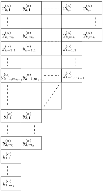
We can now rename the variables $x^{(\alpha)}_{i}$ by associating each of them to a box of the Young diagram associated with the partitions ${\mu^{(\alpha)}}$ . As a result of this renaming, we have variables $x^{(\alpha)}_{a,i,j}$ , which corresponds to the Young diagram of partition ${\mu^{(\alpha)}}$ , namely to column $j$ of the $i^{th}$ row (counted from top to bottom) of length $a$ . See the left part of figure 1 for an explicit example. In the proofs which follow, we will simplify this notation as much as possible. Note that, due to the symmetry properties of $g({\mathbf{x}})$ , how we rename the variables is irrelevant.

Let ${\mathcal{H}}$ be the space of rational functions in the variables ${\mathbf{y}}=\{y^{(\alpha)}_{a,i}\ |\ \alpha=1,\ldots,r;a\geq 1;i=1,\ldots,m^{(\alpha)}_{a}\}$ . Define the evaluation map $\varphi_{\mu^{(\alpha)}}$ , which sets all the variables in the same row of the (Young diagram associated to the) partition ${\mu^{(\alpha)}}$ to the same value, $x^{(\alpha)}_{a,i,j}\mapsto y^{(\alpha)}_{a,i}$ . The effect of the evaluation map on the variables corresponding to the partition ${\mu^{(\alpha)}}$ is shown in figure 1. We define the evaluation map $\varphi_{\boldsymbol{\mu}}:\overline{{\mathcal{F}}}\rightarrow{\mathcal{H}}$ to be $\varphi_{\boldsymbol{\mu}}=\prod_{\alpha=1}^{r}\varphi_{\mu^{(\alpha)}}$ .

Refer to caption — Figure 1. The evaluation map for the variables $x^{(\alpha)}$ . Note that we dropped the superscripts $(\alpha)$ in $m^{(\alpha)}_{a}$ .

By (3.16), $\varphi_{\boldsymbol{\mu}}(g({\mathbf{x}}))=0$ (where $g({\mathbf{x}})$ is as in (3.15) with $\overline{G}({\mathbf{x}})\in\overline{{\mathcal{F}}}$ ), if any of the partitions ${\mu^{(\alpha)}}$ has a part which is greater than $k$ . Hence, in the following, we will assume that none of the partitions has a part greater than $k$ , and refer to these (multi)-partitions as $k$ -restricted.

Our strategy will be to study the image of $\overline{{\mathcal{F}}}$ under the evaluation map.

Definition 3.5.

Let ${\mathcal{H}}_{\boldsymbol{\mu}}$ be the space of functions in the variables ${\mathbf{y}}$ , and let $\overline{{\mathcal{H}}}_{\boldsymbol{\mu}}\subset{\mathcal{H}}_{\boldsymbol{\mu}}$ be the subspace spanned by functions of the form

(3.20)

H({\mathbf{y}})=H_{\boldsymbol{\mu}}({\mathbf{y}})h({\mathbf{y}})\ ,

where $h({\mathbf{y}})$ is an arbitrary polynomial in ${\mathbf{y}}$ , symmetric under the exchange $y_{a,i}^{({\alpha})}\leftrightarrow y_{a,j}^{({\alpha})}$ , and

(3.21)

\begin{split}&H_{\boldsymbol{\mu}}({\mathbf{y}})=\\ &\prod_{\begin{subarray}{c}\alpha=1,\ldots,r\\ (a,i)>(b,j)\end{subarray}}(y^{(\alpha)}_{a,i}-y^{(\alpha)}_{b,j})^{2A_{ab}}\prod_{\begin{subarray}{c}\alpha=1,\ldots,r-1\\ (a,i);(b,j)\end{subarray}}(y^{(\alpha)}_{a,i}-y^{(\alpha+1)}_{b,j})^{-A_{ab}}\prod_{(a,i)}(y^{(\beta)}_{a,i})^{\max(0,a-l)}\ .\end{split}

Here, $A_{ab}=\min(a,b)$ and $(a,i)\in I_{k}\times I_{m_{\alpha}}$ (where $I_{m}=\{1,\ldots,m\}$ ). The ordering $(a,i)>(b,j)$ is defined as follows. The index $i$ increases downwards, and we say that $(a,i)>(b,j)$ if $a>b$ , or, if $a=b$ , when $i<j$ .

Let us define a lexicographic ordering on multi-partitions. That is, the usual lexicographic ordering is taken on partitions $\mu^{(\alpha)}$ , and ${\boldsymbol{\nu}}>{\boldsymbol{\mu}}$ if ${\nu^{(\alpha)}}={\mu^{(\alpha)}}$ for all $\alpha<\gamma$ and $\nu^{(\gamma)}>\mu^{(\gamma)}$ .

Let $\ker\varphi_{\boldsymbol{\mu}}$ be the kernel of the evaluation map $\varphi_{\boldsymbol{\mu}}$ acting on $\overline{{\mathcal{F}}}$ . We can now define the subspaces

(3.22)

\Gamma_{\boldsymbol{\mu}}=\bigcap_{\boldsymbol{\nu}>\boldsymbol{\mu}}\ker{\varphi_{\boldsymbol{\nu}}}\quad,\quad\Gamma^{\prime}_{\boldsymbol{\mu}}=\bigcap_{\boldsymbol{\nu}\geq\boldsymbol{\mu}}\ker{\varphi_{\boldsymbol{\nu}}}\ .

Thus, $\Gamma_{{\boldsymbol{\mu}}}$ is the space of rational functions which are annihilated by every evaluation map with ${\boldsymbol{\nu}}>{\boldsymbol{\mu}}$ .

By definition, $\Gamma_{{\boldsymbol{\nu}}}\subset\Gamma_{{\boldsymbol{\mu}}}$ if ${\boldsymbol{\nu}}<{\boldsymbol{\mu}}$ , and $\Gamma^{\prime}_{{\boldsymbol{\mu}}}\subset\Gamma_{{\boldsymbol{\mu}}}$ . In addition, $\Gamma^{\prime}_{(1^{m^{(1)}},\ldots,1^{m^{(r)}})}=\{0\}$ . Therefore, $\Gamma_{\boldsymbol{\mu}}$ defines a filtration on $\overline{{\mathcal{F}}}$ . Define the associated graded space

(3.23)

\Gr\Gamma=\bigoplus_{{\boldsymbol{\mu}}}\Gr_{{\boldsymbol{\mu}}}\Gamma\ ,

where $\Gr_{{\boldsymbol{\mu}}}\Gamma=\Gamma_{{\boldsymbol{\mu}}}/\Gamma^{\prime}_{{\boldsymbol{\mu}}}$ and the sum is over multi-partitions of ${\mathbf{m}}$ . The main purpose of this section is to prove

Theorem 3.6.

The induced map

(3.24)

\overline{\varphi}_{{\boldsymbol{\mu}}}:\Gr_{{\boldsymbol{\mu}}}\Gamma\rightarrow\overline{{\mathcal{H}}}_{\boldsymbol{\mu}}

is an isomorphism of graded vector spaces.

This is very similar to the proof found in [7] for the case which corresponds to $\widehat{{\mathfrak{sl}}}_{3}$ , and we use the same ideas here.

To prove the theorem, we need to show three things. First, the evaluation map

(3.25)

{\varphi}_{\boldsymbol{\mu}}:\Gamma_{\boldsymbol{\mu}}\rightarrow\overline{{\mathcal{H}}}_{\boldsymbol{\mu}}

is well-defined. Second, it is surjective, and third, the induced map (3.24) is well defined and injective.

3.4.1. The evaluation map is well-defined

To prove that the map $\varphi_{\boldsymbol{\mu}}:\Gamma_{\boldsymbol{\mu}}\rightarrow\overline{{\mathcal{H}}}_{\boldsymbol{\mu}}$ , is well defined, we must show that the rational functions obtained after the evaluation are indeed of the form (3.20) and (3.21). We will do this by showing that the structure of the poles and zeros of the image of the functions (3.19) in $\overline{{\mathcal{F}}}_{\mathbf{m}}$ under the evaluation map is precisely of the form (3.21).

Lemma 3.7.

Let $\overline{G}({\mathbf{x}})\in\Gamma_{\boldsymbol{\mu}}$ . Then, the function $\varphi_{\boldsymbol{\mu}}(\overline{G}({\mathbf{x}}))$ has a zero of order at least $2\min(a,a^{\prime})$ when $y^{(\alpha)}_{a,i}=y^{(\alpha)}_{a^{\prime},i^{\prime}}\ ,\ \forall\alpha$ .

Proof.

The proof is independent of $\alpha$ , and so we can use the argument used in the case of $\widehat{{\mathfrak{sl}}}_{2}$ in [2]. We will repeat that argument here for completeness.

It is sufficient to consider the dependence of $\overline{G}({\mathbf{x}})$ on the two sets of variables of the same color $\alpha$ , which we denote by $\{x_{a,i}\ |\ i=1,\ldots,a\}$ and $\{x_{a^{\prime},i^{\prime}}\ |\ i^{\prime}=1,\ldots,a^{\prime}\}$ . We can assume that $a\geq a^{\prime}$ without loss of generality.

We can carry out the evaluation map in two steps: $\varphi_{{\boldsymbol{\mu}}}=\varphi^{2}\circ\varphi^{1}$ . Here $\varphi^{1}$ consists of evaluating all the variables except the set $\{x_{a^{\prime},i^{\prime}}\ |\ i^{\prime}=1,\ldots,a^{\prime}\}$ and $\varphi^{2}$ consists of setting $x_{a^{\prime},1}=\cdots=x_{a^{\prime},a^{\prime}}=y_{a^{\prime}}$ (note that under $\varphi^{1}$ , the variables $x_{a,1},\ldots,x_{a,a}$ are all set to $y_{a}$ ).

Let

(3.26)

g_{1}(y_{a};x_{a^{\prime},1},\ldots,x_{a^{\prime},a^{\prime}})=\varphi^{1}(\overline{G}({\mathbf{x}}))\ .

Because $\overline{G}({\mathbf{x}})\in\Gamma_{\boldsymbol{\mu}}$ , $\overline{G}({\mathbf{x}})$ is annihilated by all $\varphi_{{\boldsymbol{\nu}}}$ with ${\boldsymbol{\nu}}>{\boldsymbol{\mu}}$ . Therefore

(3.27)

\left.g_{1}(y_{a};x_{a^{\prime},1},\ldots,x_{a^{\prime},a^{\prime}})\right|_{x_{a^{\prime},i^{\prime}}=y_{a}}=0\ \hbox{for all $i^{\prime}$},

because this corresponds to an evaluation corresponding to a multi-partition greater than ${\boldsymbol{\mu}}$ . Therefore,

(3.28)

g_{1}(y_{a};x_{a^{\prime},1},\ldots,x_{a^{\prime},a^{\prime}})=\prod_{i^{\prime}=1}^{a^{\prime}}(x_{a}-x_{a^{\prime},i^{\prime}})\tilde{g}_{1}(y_{a};x_{a^{\prime},1},\ldots,x_{a^{\prime},a^{\prime}})\ .

Now $g_{1}(y_{a};x_{a^{\prime},1},\ldots,x_{a^{\prime},a^{\prime}})$ was obtained from a symmetric function in $x_{i}^{({\alpha})}$ , and so, for each $i^{\prime}$ ,

(3.29)

\left.\frac{\partial g_{1}}{\partial y_{a}}\right|_{x_{a^{\prime},i^{\prime}}=y_{a}}=a\left.\frac{\partial g_{1}}{\partial x_{a^{\prime},i^{\prime}}}\right|_{x_{a^{\prime},i^{\prime}}=y_{a}}\ .

However (3.28) tells us that, again for each $i^{\prime}$ ,

(3.30)

\left.\frac{\partial g_{1}}{\partial y_{a}}\right|_{x_{a^{\prime},i^{\prime}}=y_{a}}=-\left.\frac{\partial g_{1}}{\partial x_{a^{\prime},i^{\prime}}}\right|_{x_{a^{\prime},i^{\prime}}=y_{a}}=\left.\sideset{}{{}^{\prime}}{\prod}_{i^{\prime\prime}=1}^{a^{\prime}}(y_{a}-x_{a^{\prime},i^{\prime\prime}})\tilde{g}_{1}\right|_{x_{a^{\prime},i^{\prime}}=y_{a}}\ ,

the prime on the product meaning that the term with $i^{\prime\prime}=i^{\prime}$ is to be omitted. The only way to reconcile (3.29) with (3.30) is for $\tilde{g}_{1}|_{x_{a^{\prime},i^{\prime}}=y_{a}}$ to be zero. Thus the zero at $x_{a^{\prime},i^{\prime}}=y_{a}$ is at least of order two

(3.31)

g_{1}(y_{a};x_{a^{\prime},1},\ldots,x_{a^{\prime},a^{\prime}})=\prod_{i^{\prime}=1}^{a^{\prime}}(y_{a}-x_{a^{\prime},i^{\prime}})^{2}\tilde{g}_{2}(u_{a};x_{a^{\prime},1},\ldots,x_{a^{\prime},a^{\prime}})\ .

We now evaluate the right-hand-side of (3.31) at $x_{a^{\prime},1}=\cdots=x_{a^{\prime},a^{\prime}}=y_{a^{\prime}}$ and, recalling the condition that $a\geq a^{\prime}$ , we have

(3.32)

\varphi_{\boldsymbol{\mu}}(G({\mathbf{x}}))=\prod(y_{a}-y_{a^{\prime}})^{2A_{a,a^{\prime}}}\widetilde{G}\ .

∎

Lemma 3.8.

The image under the evaluation map $\varphi_{\boldsymbol{\mu}}$ of any function in $\overline{{\mathcal{F}}}$ (and hence $\Gamma_{\boldsymbol{\mu}}$ ) has a pole of maximal order $\min(a,a^{\prime})$ whenever $y^{(\alpha)}_{a,i}=y^{(\alpha+1)}_{a^{\prime},i^{\prime}}$ .

Proof.

We will prove this lemma by looking at the zeros of ${g}({\mathbf{x}})$ , which arise because we need to satisfy the Serre relations, ${g}|_{x^{(\alpha)}_{1}=x^{(\alpha)}_{2}=x^{(\alpha+1)}_{1}}=0$ and ${g}|_{x^{(\alpha)}_{1}=x^{(\alpha+1)}_{1}=x^{(\alpha+1)}_{2}}=0$ for $\alpha=1,\ldots,r-1$ . These relations depend on two sets of variables only.

Consider the dependence of ${g}$ on the two sets of variables $x_{i}=x^{(\alpha)}_{i}$ , with $i=1,\ldots,a$ and $\bar{x}_{j}=x^{({\alpha}\pm 1)}_{j}$ , with $j=1,\ldots,a^{\prime}$ . Under the evaluation map, these variables map to $\varphi_{\boldsymbol{\mu}}(x_{i})=y$ and $\varphi_{\boldsymbol{\mu}}(\bar{x}_{i})=\bar{y}$ respectively.

Note that $x$ and $\bar{x}$ are variables corresponding to two adjacent roots. Again without loss of generality, assume that $a\geq a^{\prime}$ .

When $x_{1}=\bar{x}_{1}=\bar{x}_{j}$ or $x_{1}=x_{j}=\bar{x}_{1}$ , ${g}$ vanishes, so we find

(3.33)

\begin{split}&{g}(x_{1},\ldots,x_{a};\bar{x}_{1},\ldots,\bar{x}_{a^{\prime}};\ldots)|_{x_{1}=\bar{x}_{1}=z_{1}}=\\ &\prod_{i=2}^{a}(x_{i}-z_{1})\prod_{j=2}^{a^{\prime}}(\bar{x}_{i}-z_{1}){g}^{\prime}(z_{1};x_{2},\ldots,x_{a};\bar{x}_{2},\ldots,\bar{x}_{a^{\prime}};\ldots)\end{split}

Repeating the argument for ${g}^{\prime}$ we find

(3.34)

\begin{split}&{g}^{\prime}(x_{2},\ldots,x_{a};\bar{x}_{2},\ldots,\bar{x}_{a^{\prime}};\ldots)|_{x_{2}=\bar{x}_{2}=z_{2}}=\\ &\prod_{i=3}^{a}(x_{i}-z_{2})\prod_{j=3}^{a^{\prime}}(\bar{x}_{i}-z_{2}){g}^{\prime\prime}(z_{1},z_{2};x_{3},\ldots,x_{a};\bar{x}_{3},\ldots,\bar{x}_{a^{\prime}};\ldots)\end{split}

We can repeat this argument $a^{\prime}$ times with the result

(3.35)

\begin{split}&{g}(x_{1},\ldots,x_{a};\bar{x}_{1},\ldots,\bar{x}_{a^{\prime}};\ldots)|_{\{x_{i}=\bar{x}_{i}=z_{i}\}_{i=1}^{a^{\prime}}}=\\ &\prod_{i=1}^{a^{\prime}}\prod_{j=i+1}^{a}(x_{j}-z_{i})\prod_{i=1}^{a^{\prime}}\prod_{j^{\prime}=i+1}^{a^{\prime}}(\bar{x}_{j^{\prime}}-z_{i})\tilde{g}(z_{1},\ldots,z_{a^{\prime}};x_{a^{\prime}+1},\ldots,x_{a};\ldots)\ .\end{split}

We find that $\varphi_{\boldsymbol{\mu}}({g})$ has a zero of order at least $aa^{\prime}-\min(a,a^{\prime})$ when $y=\bar{y}$ , by counting the number of zeros in (3.35) and using that $a^{\prime}\leq a$ . Taking into account the poles of (3.19), which after applying the evaluation map becomes a pole of order $aa^{\prime}$ when $y=\bar{y}$ , we find that the image of $\overline{{\mathcal{F}}}_{\mathbf{m}}$ has a pole or order at most $\min(a,a^{\prime})$ , when $x^{(\alpha)}_{a,j}=x^{({\alpha}\pm 1)}_{a^{\prime},j^{\prime}}$ . ∎

Lemma 3.9.

The image of $\varphi_{{\boldsymbol{\mu}}}$ acting on a function $\overline{G}\in\Gamma_{\boldsymbol{\mu}}$ has a zero of order at least $\max(0,a-l)$ when $y^{(\beta)}_{a,i}=0$ .

Proof.

To prove this lemma, we will study the effect of the evaluation map on ${g}({\mathbf{x}})$ in eq. (3.15). We focus on the variables of a row of length $a$ (where we assume that $a>l$ ), $\{x^{(\beta)}_{j}\ |\ j=1,\ldots,a\}$ . Under the evaluation map, these variables map to $\varphi_{\boldsymbol{\mu}}(x^{(\beta)}_{j})=y^{(\beta)}$ .

We know that the function

(3.36)

g_{1}(x^{(\beta)}_{1},\ldots,x^{(\beta)}_{a})=g({\mathbf{x}})|_{x^{(\beta)}_{1}=\cdots=x^{(\beta)}_{l}=0}

contains a factor $\prod_{j=l+1}^{a}x^{(\beta)}_{j}$ , because it vanishes if any of the remaining variables $x^{(\beta)}_{j}$ is set to zero (because of the condition (3.18) on ${g}({\mathbf{x}})$ ). Thus, the image of $g_{1}$ under the evaluation map has a zero of order at least $\max(0,a-l)$ whenever $y^{(\beta)}_{a,i}=0$ . ∎

Lemma 3.10.

The map $\varphi_{\boldsymbol{\mu}}:\Gamma_{\boldsymbol{\mu}}\rightarrow\overline{{\mathcal{H}}}_{\boldsymbol{\mu}}$ is well defined.

Proof.

This follows from the lemmas 3.7, 3.8, 3.9 and the definition of the space $\overline{{\mathcal{H}}}_{\boldsymbol{\mu}}$ . ∎

3.4.2. Proof of surjectivity

We will continue with the proof that the map (3.25) is surjective. We have to prove that for each function of the form defined by (3.20) and (3.21), there is at least one function in the pre-image in $\Gamma_{\boldsymbol{\mu}}$ . We do this by explicitly giving the form of these pre-images, showing that they are elements of $\overline{{\mathcal{F}}}$ and finally, proving that these pre-images are indeed in the kernel of $\varphi_{\boldsymbol{\nu}}$ for each ${\boldsymbol{\nu}}>{\boldsymbol{\mu}}$ , which shows that they are in $\Gamma_{\boldsymbol{\mu}}$ .

For each ( $k$ -restricted) multi-partition ${\boldsymbol{\mu}}$ , we consider the function

(3.37)

F({\mathbf{x}})=\frac{\sym f({\mathbf{x}})}{p({\mathbf{x}})}\ ,

where $f({\mathbf{x}})$ and $p({\mathbf{x}})$ are a polynomials of the form (we identify the variables $x^{(\alpha)}_{a,i,a+1}=x^{(\alpha)}_{a,i,1}$ )

(3.38)		$\displaystyle f({\mathbf{x}})$	$\displaystyle=\tilde{f}({\mathbf{x}})\prod_{\begin{subarray}{c}\alpha,a,i\\ j>l\end{subarray}}x^{(\beta)}_{a,i,j}\prod_{\begin{subarray}{c}\alpha\\ a,i,j\\ a^{\prime},i^{\prime};j^{\prime}\neq j\end{subarray}}(x^{(\alpha)}_{a,i,j}-x^{(\alpha+1)}_{a^{\prime},i^{\prime},j^{\prime}})\prod_{\begin{subarray}{c}\alpha\\ (a,i)>(a^{\prime},i^{\prime})\\ j=1,\ldots,m^{(\alpha)}_{a^{\prime}}\end{subarray}}(x^{(\alpha)}_{a,i,j}-x^{(\alpha)}_{a^{\prime},i^{\prime},j})(x^{(\alpha)}_{a,i,j+1}-x^{(\alpha)}_{a^{\prime},i^{\prime},j})$
(3.39)		$\displaystyle p({\mathbf{x}})$	$\displaystyle=\prod_{\begin{subarray}{c}\alpha=1,\ldots,r-1\\ a,i,j\\ a^{\prime},i^{\prime},j^{\prime}\end{subarray}}(x^{(\alpha)}_{a,i,j}-x^{(\alpha+1)}_{a^{\prime},i^{\prime},j^{\prime}})\ ,$

where $\tilde{f}({\mathbf{x}})$ is an arbitrary polynomial. The symmetrization is over each of the $r$ sets of variables $\{x^{(\alpha)}_{i}\}$ with the same value of $\alpha$ . As we did before, we will drop as many indices as possible in the following lemmas.

Lemma 3.11.

The functions $F({\mathbf{x}})$ of (3.37) are elements of $\overline{{\mathcal{F}}}$

Proof.

We have to show that $f({\mathbf{x}})$ satisfies the vanishing conditions (3.16), (3.17) and (3.18). First of all, we easily see that $f({\mathbf{x}})$ is zero when any $k+1$ variables of the same color are set to the same value. Because the partitions have rows of maximum length $k$ , these $k+1$ variables can not all be placed in the same row, which implies that the factor $\prod(x^{(\alpha)}_{a,i,j}-x^{(\alpha)}_{a^{\prime},i^{\prime},j^{\prime}})$ evaluates to zero under $\varphi_{\boldsymbol{\mu}}$ .

To show that the Serre relations are satisfied, we have to show that the zeros

(3.40)

\prod_{\begin{subarray}{c}\alpha\\ a,i,j\\ a^{\prime},i^{\prime};j^{\prime}\neq j\end{subarray}}(x^{(\alpha)}_{a,i,j}-x^{(\alpha+1)}_{a^{\prime},i^{\prime},j^{\prime}})

satisfy the Serre relations. Let $x_{a,j}=x^{(\alpha)}_{a,i,j}$ and $\bar{x}_{a^{\prime},j^{\prime}}=x^{(\alpha+1)}_{a^{\prime},i^{\prime},j^{\prime}}$ , for some choice of $\alpha$ , $i$ and $i^{\prime}$ .

For every $x$ , there is a zero with every $\bar{x}$ , except those appearing in the column which has the same number as the $x$ (i.e. for $j=j^{\prime}$ ). Note that if we set two variables $x$ , which belong to the same column, to the same value, $f({\mathbf{x}})$ is zero, because the factor $\prod(x^{(\alpha)}_{a,i,j}-x^{(\alpha)}_{a^{\prime},i^{\prime},j^{\prime}})$ is zero in that case. Hence, we set $x_{a,j}=\bar{x}_{a^{\prime},j^{\prime}}=\tilde{x}\ (j^{\prime}\neq j)$ . Focusing on this variable, we find the following zeros $(\tilde{x}-\bar{x}_{a,i})(\tilde{x}-\bar{x}_{a^{\prime},i^{\prime}})\prod_{a^{\prime\prime};i^{\prime\prime}\neq i,i^{\prime}}(\tilde{x}-\bar{x}_{a^{\prime\prime},i^{\prime\prime}})^{2}$ So, indeed $\tilde{x}$ has zero with every $\bar{x}$ . Similarly, we find that there is at least a zero of order one when we set $x_{1}=\bar{x}_{1}=\bar{x}_{2}$ .

To complete the proof of this lemma, we need to show that $f({\mathbf{x}})$ satisfies the condition (3.18). This easily follows form the factor $\prod_{j>l}x^{(\beta)}_{a,i,j}$ , combined with the zeros which give rise to the condition (3.16). ∎

Remark 3.12.

It is instructive to note that all the zeros in (3.40) are necessary to satisfy the Serre relations. We need to show that if we remove any of these zeros, we will violate a Serre relation.

To show that this is true, it is important that we take the zeros between variables of the same color into account. Let us remove the zero $(x_{a,j}-\bar{x}_{a^{\prime},j^{\prime}})$ , where $j\neq j^{\prime}$ . Without loss of generality, we can assume that $j<j^{\prime}$ . The two variables are indicated in figure 2 by the black boxes. The gray boxes denote the zeros with the variables corresponding to the black box from the same partition.

All we need to do is show that there is at least one variable, of either partition, such that when this variable is set to the same value as the two ‘black variables’, we do not get a zero, and thus violate a Serre relation. This variable is taken to be of color $(\alpha+1)$ , (if $j>j^{\prime}$ , it is of color $(\alpha)$ ). More precisely, it is the variable $\bar{x}_{a^{\prime},j}$ , taken from the same row as $\bar{x}_{a^{\prime},j^{\prime}}$ (denoted by the ‘slanted’ box), which always exists, because $j<j^{\prime}$ .

There is no zero at $\bar{x}_{a^{\prime},j^{\prime}}=\bar{x}_{a^{\prime},j}$ , because both variables are taken from the same row. In addition, there is no zero at $x_{a,j}=\bar{x}_{a^{\prime},j}$ , because it is not present in the factor (3.40) and the zero at $x_{a,j}=\bar{x}_{a^{\prime},j^{\prime}}$ is the one we removed. We conclude that after we remove the (arbitrary) zero at $x_{a,j}=\bar{x}_{a^{\prime},j^{\prime}}$ , we do not have a zero when $x_{a,j}=\bar{x}_{a^{\prime},j^{\prime}}=\bar{x}_{a^{\prime},j}$ . Thus, we have shown that by removing any of the zeros in (3.40), we violate a Serre condition. We conclude that the zeros are indeed necessary.

Lemma 3.13.

The function $F({\mathbf{x}})$ of (3.37) associated to a $k$ -restricted multi-partition ${\boldsymbol{\mu}}$ is an element of the kernel of $\varphi_{\boldsymbol{\nu}}$ for any ${\boldsymbol{\nu}}>{\boldsymbol{\mu}}$ .

Proof.

Let us take a ${\boldsymbol{\nu}}>{\boldsymbol{\mu}}$ , and let ${\nu^{(\alpha)}}$ be the first partition such that ${\nu^{(\alpha)}}>{\mu^{(\alpha)}}$ . We will focus on the variables $x^{(\alpha)}$ and show that the function $F({\mathbf{x}})$ can not be non-zero under the evaluation map $\varphi_{\boldsymbol{\nu}}$ .

Two variables in the same column of ${\mu^{(\alpha)}}$ have a zero, so they can not be placed in the same row in ${\nu^{(\alpha)}}$ , if the result is to be non-zero, because in that case, acting with the evaluation map gives a zero.

However, because ${\nu^{(\alpha)}}>{\mu^{(\alpha)}}$ , we can not avoid placing variables of the same column in ${\mu^{(\alpha)}}$ in the same row of ${\nu^{(\alpha)}}$ . To show this, let us denote the length of the rows of the partitions by $\mu^{(\alpha)}_{i}$ and $\nu^{(\alpha)}_{i}$ , such that the index $i$ is increasing going downwards. The only way to avoid placing variables of the same column of ${\mu^{(\alpha)}}$ in the same row of ${\nu^{(\alpha)}}$ is by placing the variables of ${\mu^{(\alpha)}}$ in a rows of the same length in ${\nu^{(\alpha)}}$ . However, because ${\nu^{(\alpha)}}>{\mu^{(\alpha)}}$ , there will be an $\tilde{\imath}$ such that $\nu^{(\alpha)}_{\tilde{\imath}}>\mu^{(\alpha)}_{\tilde{\imath}}$ . Let us focus on the smallest $\tilde{\imath}$ . We have to place a variable of a row $\mu^{({\alpha})}_{i}$ with $i>\tilde{\imath}$ in the row $\nu^{({\alpha})}_{\tilde{i}}$ . Because $\mu^{(\alpha)}_{i}\leq\mu^{(\alpha)}_{\tilde{\imath}}$ , this variable belongs to the same column of another variable in $\nu^{(\alpha)}_{\tilde{\imath}}$ . We conclude that $F({\mathbf{x}})$ is zero under the evaluation map $\varphi_{\boldsymbol{\nu}}$ with ${\boldsymbol{\nu}}>{\boldsymbol{\mu}}$ . ∎

Lemma 3.14.

The function $F({\mathbf{x}})$ of (3.37) is an element of $\Gamma_{\boldsymbol{\mu}}$ .

Proof.

This follows from the lemmas 3.11 and 3.13 ∎

As a last step in the proof of surjectivity, we have to show that the image of $F({\mathbf{x}})$ under the evaluation map is indeed of the form (3.20) and (3.21). In particular, it contains as a factor the functions $h({\mathbf{y}})$ , which are symmetric under the exchange of variables $y^{(\alpha)}_{a,i}\leftrightarrow y^{(\alpha)}_{a,i^{\prime}}$ .

Lemma 3.15.

The image of $F({\mathbf{x}})$ under the evaluation map $\varphi_{{\boldsymbol{\mu}}}$ is a scalar multiple of the function $H({\mathbf{y}})$ in (3.20).

Proof.

To prove this lemma, we can follow the same approach as we did in our paper on the $\widehat{\mathfrak{sl}}_{2}$ case, because the argument does not depend on the color of the variables. We will focus on the variables $x^{(\alpha)}$ , and determine the permutations $\sigma$ , for which $\varphi_{\boldsymbol{\mu}}(f(\sigma(x^{(\alpha)})))$ is non-zero. So, we consider

(3.41)

\sum_{\sigma\in{\mathcal{S}}_{m^{(\alpha)}}}f(\sigma\{x^{(\alpha)}\})\ .

In the following, we will omit the label $\alpha$ . Recall that the variable $x_{a,i,j}$ corresponds to the $j^{th}$ column in the $i^{th}$ row of length $a$ . Under the evaluation map, $x_{a,i,j}\mapsto y_{a,i}\;\forall j$ .

Suppose that for some $\sigma$ , we have $\sigma(x_{a,i,j})=x_{a^{\prime},i^{\prime},j^{\prime}}$ with $(a^{\prime},i^{\prime})<(a,i)$ and that $(a,i)$ is the largest row for which this is true. This means that all rows above $(a,i)$ undergo only a permutation within the row. Suppose that the pre-factor

(3.42)

\varphi_{\boldsymbol{\mu}}\circ\sigma\left(\prod_{(a,i)>(a^{\prime},i^{\prime})}(x_{a,i,j}-x_{a^{\prime},i^{\prime},j})(x_{a,i,j+1}-x_{a^{\prime},i^{\prime},j})\right)

is to be non-zero. Then $x_{a^{\prime},i^{\prime},j^{\prime}}$ can not be in a column directly below or to the left of the permutation image of any other element from row $(a,i)$ . This means that at least one other element from row $(a,i)$ should be mapped to a row below $(a,i)$ . If it is mapped to the row $(a^{\prime},i^{\prime})$ it can appear in any column other than $j^{\prime}$ . If it mapped to any other row, it can appear in any other column than $j^{\prime}$ and an adjacent column (to the right or left depending on whether it is above or below $(a^{\prime},i^{\prime})$ .) Now we repeat this argument for this new element, concluding that at least one more element of row $(a,i)$ is mapped to a lower row, and so forth, until eventually we find that all elements are permuted to a row below $(a,i)$ . If the elements are permuted to the same row, they can be placed adjacent columns. Elements which are permuted to different rows can not be placed in adjacent columns, this being due to the factor linking adjacent columns in the pre-factor. There are at most $a$ columns in $\mu^{(\alpha)}$ in rows below $(a,i)$ , and hence the elements must all appear in the same row, which is therefore of length $a$ . Thus all the variables in rows of length $a$ are mapped to another row of length $a$ , for the same reason. As a result, the only permutations which give a non-zero contribution to $\varphi_{\boldsymbol{\mu}}(f(\sigma(x^{(\alpha)})))$ are those that permute variables within each row, or those that permute rows of equal length. Under the evaluation map, the former contribute equal terms to the sum, while row interchanges correspond to the symmetrization over the variables $y^{(\alpha)}_{a,i}$ with the same values of $\alpha$ and $a$ in $h({\mathbf{y}})$ . Note that the other factors in the function $F$ are symmetric under the permutation of rows of equal length, so these factors do not interfere with the argument above. ∎

Lemma 3.16.

The map $\varphi_{{\boldsymbol{\mu}}}:\Gamma_{\boldsymbol{\mu}}\rightarrow\overline{{\mathcal{H}}}_{\boldsymbol{\mu}}$ is surjective.

Proof.

This follows from the lemmas 3.14 and 3.15. ∎

3.4.3. Injectivity proof

Lemma 3.17.

The induced map $\overline{\varphi}_{{\boldsymbol{\mu}}}:\Gr_{{\boldsymbol{\mu}}}\Gamma\rightarrow\overline{{\mathcal{H}}}_{\boldsymbol{\mu}}$ (3.24) is well defined and injective.

Proof.

To prove that the map (3.24) is well defined, we use lemma 3.10 and observe that the image of $\Gamma^{\prime}_{{\boldsymbol{\mu}}}$ under $\varphi_{{\boldsymbol{\mu}}}$ is zero by using the definition of $\Gamma^{\prime}_{{\boldsymbol{\mu}}}$ . It follows that we can define the induced map $\overline{\varphi}_{\boldsymbol{\mu}}$ acting on the quotient $\Gr_{{\boldsymbol{\mu}}}\Gamma=\Gamma_{{\boldsymbol{\mu}}}/\Gamma^{\prime}_{{\boldsymbol{\mu}}}$ . Moreover, the difference between two different functions in $\Gamma_{{\boldsymbol{\mu}}}$ that map to the same rational function in $\overline{{\mathcal{H}}}_{\boldsymbol{\mu}}$ is in $\Gamma_{{\boldsymbol{\mu}}}$ . Hence, the map is also injective. ∎

We have now completed the proof of theorem 3.6, because the theorem follows from the lemmas 3.17 and 3.16.

The map (3.24) is degree preserving, and thus we can count the functions of homogeneous degree $d$ in $\overline{{\mathcal{H}}}_{\boldsymbol{\mu}}$ to obtain the character of the space $\overline{{\mathcal{F}}}$ .

To compute the character of ${\mathcal{F}}_{\lambda}$ , we add the poles $\prod(x^{(\beta)}_{a,i,j})^{-1}$ , which are present in the functions $G({\mathbf{x}})$ in (3.15). The only thing in the calculation of the character which changes is the fact that due to these poles, the zeros $\prod(y^{(\beta)}_{a,i})^{\max(0,a-l)}$ in (3.21) become poles $\prod(y^{(\beta)}_{a,i})^{-\min(a,l)}$ .

3.5. Character of the dual space

Using the results of the previous section, we can calculate the character of the dual space ${\mathcal{F}}_{\lambda}$ , where $\lambda=l\omega_{\beta}$ .

First, let us define the character of $W_{\lambda}$ as follows:

(3.43)

{\rm ch}_{q}W_{\lambda}=\sum_{d,m^{(\alpha)}}\dim W_{\lambda}[\mathbf{m}]_{d}\ q^{d}e^{\lambda-{\boldsymbol{\omega}}^{T}C_{r}{\mathbf{m}}},

where $W_{\lambda}[\mathbf{m}]_{d}$ is the subspace generated by elements in $U({\widetilde{{\mathfrak{n}}}_{-}})$ of homogeneous degree $m^{(\alpha)}$ in $f_{\alpha}$ , and homogeneous degree $-d$ in $t$ . Here, ${\boldsymbol{\omega}}=(\omega_{1},\ldots,\omega_{r})^{T}$ .

The space $\mathcal{F}_{\lambda}$ is a space of functions in the variables $x_{i}^{(\alpha)}$ . If we define its $(\mathbf{m},d)$ -graded component to be the space of functions in $m^{(\alpha)}$ variables $x_{i}^{(\alpha)}$ and total homogeneous degree $\widetilde{d}$ in all the variables, then, due to the way we defined the generating functions $f_{\alpha}(x)$ (or, equivalently, the coupling), we have that $\mathcal{F}_{\lambda}[\mathbf{m}]_{\widetilde{d}}$ is the dual to $W_{\lambda}[\mathbf{m}]_{d}$ where $d=\widetilde{d}+\sum_{\alpha}m^{(\alpha)}$ .

Thus,

(3.44)

{\rm ch}_{q}W_{\lambda}=\sum_{{\mathbf{m}}}{\rm ch}W_{\lambda}[{\mathbf{m}}]=\sum_{\mathbf{m}}\sum_{d}q^{d+\sum_{\alpha}m^{(\alpha)}}e^{\lambda-{\boldsymbol{\omega}}^{T}C_{r}{\mathbf{m}}}\dim({\mathcal{F}}_{\lambda}[{\mathbf{m}}])_{d}\ ,

where $\dim({\mathcal{F}}_{\lambda}[{\mathbf{m}}])_{d}$ denotes the dimension of the subspace of functions in ${\mathcal{F}}_{\lambda}[{\mathbf{m}}]$ which have homogeneous degree $d$ . The powers of $z$ correspond to the components of the weights in terms of the simple roots. Recall that here, $\lambda=\lambda_{\beta}=l\omega_{\beta}$ .

We will calculate this character by actually summing over all the functions in ${\mathcal{H}}$ , and counting their homogeneous degree. The character of the space of symmetric functions $h({\mathbf{y}})$ in $m_{a}^{({\alpha})}$ variables is given by

(3.45)

\frac{1}{\prod_{\alpha=1}^{r}\prod_{a=1}^{k}(q)_{m^{(\alpha)}_{a}}}\ ,

where $(q)_{m}=\prod_{i=1}^{m}(1-q^{i})$ for $m\in{\mathbb{N}}$ and $(q)_{0}=1$ .

The homogeneous degree of the rational function $H_{\boldsymbol{\mu}}({\mathbf{y}})$ , combined with the additional poles ${\prod_{(a,i)}(y^{(\alpha)}_{a,i})^{-a}}$ is given by

(3.46)

\deg\left(\frac{H_{\boldsymbol{\mu}}({\mathbf{y}})}{\prod_{(a,i)}(y^{(\alpha)}_{a,i})^{a}}\right)=\sum_{\alpha,\alpha^{\prime},a,a^{\prime}}\frac{1}{2}m_{a}^{(\alpha)}(C_{r})_{\alpha,\alpha^{\prime}}A_{a,a^{\prime}}m_{a^{\prime}}^{(\alpha^{\prime})}-\sum_{a}A_{a,l}m_{a}^{(\beta)}-\sum_{\alpha}m^{(\alpha)}\ .

It follows that the character of $W_{\lambda}^{(0)}$ is

(3.47)

{\rm ch}_{q}W_{l\omega_{\beta}}^{(0)}=\sum_{{\overset{\to}{{\mathbf{m}}}}\in{\mathbb{Z}}_{\geq 0}^{r\times k}}\frac{q^{\frac{1}{2}{{\overset{\to}{{\mathbf{m}}}}}^{T}(C_{r}\otimes A){{\overset{\to}{{\mathbf{m}}}}}-({\rm id}\otimes A{\overset{\to}{{\mathbf{m}}}})_{l}^{(\beta)}}}{(q)_{{\overset{\to}{{\mathbf{m}}}}}}e^{l\omega_{\beta}-{\boldsymbol{\omega}}^{T}C_{r}{\mathbf{m}}}.

Here $(A)_{a,b}=\min(a,b)$ is a $k\times k$ matrix, and $C_{r}$ is the Cartan matrix of ${\mathfrak{sl}}_{r+1}$ . Also, ${\overset{\to}{{\mathbf{m}}}}$ denotes the vector $(m_{1}^{(1)},\ldots,m_{k}^{(1)};\cdots;m_{1}^{(r)},\ldots,m_{k}^{(r)})$ . We made use of the definition

(q)_{{\overset{\to}{{\mathbf{m}}}}}={\prod_{\alpha=1}^{r}\prod_{a=1}^{k}(q)_{m_{a}^{(\alpha)}}}\ .

4. Characters for rectangular highest-weight $\widehat{{\mathfrak{sl}}}_{r+1}$ -modules

In this section, we will show that we can use the characters of the principal subspace $W_{\lambda}$ to obtain the character of the full integrable module $V_{\lambda}$ . We will be able to do this by using the invariance of the weight multiplicities of $V_{\lambda}$ under the action of the affine Weyl group, in particular the affine Weyl translations $t_{\alpha}$ . More specifically, we will show that acting with an affine Weyl translation on the principal subspace, and taking an appropriate limit, we obtain the full integrable module.

Let $\Lambda$ be an affine weight of level $k$ . It can be written as

\Lambda=\lambda+k\Lambda_{0}-m\delta,

where $\lambda$ is the weight with respect to ${\mathfrak{h}}\in{\mathfrak{sl}}_{r+1}$ . Let $t_{\alpha}$ be the affine Weyl translation corresponding to the root $\alpha$ (see [11], equation (6.5.2)), and define the translation $t_{\mathbf{N}}=\prod_{i}t_{N_{i}\alpha_{i}}$ , where ${\mathbf{N}}=(N_{1},\ldots,N_{r})^{T}$ . Then

(4.1)

t_{{\mathbf{N}}}(\Lambda)=\lambda+k{\mathbf{N}}^{T}\cdot\boldsymbol{\alpha}+k\Lambda_{0}-(m+{\mathbf{N}}^{T}\cdot\mathbf{l}+\frac{1}{2}k{\mathbf{N}}^{T}C_{r}{\mathbf{N}})\delta.

Again, $\mathbf{l}=(l_{1},\ldots,l_{r})^{T}$ where $\lambda=\sum_{i}l_{i}\omega_{i}$ , and $\boldsymbol{\alpha}=(\alpha_{1},\ldots,\alpha_{r})^{T}$ . Also note that ${\boldsymbol{\alpha}}$ in terms of the weights is given by ${\boldsymbol{\alpha}}=C_{r}{\boldsymbol{\omega}}$ .

Consider the principal subspace $W^{({\mathbf{N}})}=U({\widetilde{{\mathfrak{n}}}_{-}})t_{{\mathbf{N}}}v_{\lambda}$ . It has a dual space description which is similar to ${\mathcal{F}}_{\lambda}$ , if we choose the vector ${\mathbf{N}}$ carefully. Given that if $f_{\alpha}[m]v_{\lambda}=0$ , then $f_{\alpha}[m+(C_{r}\cdot{\mathbf{N}})_{\alpha}]t_{{\mathbf{N}}}v_{\lambda}=0$ (since the Weyl group preserves weight space multiplicities), we choose ${\mathbf{N}}$ such that $(C_{r}\cdot{\mathbf{N}})_{\alpha}=2N$ for all ${\alpha}$ , for some $N\in{\mathbb{Z}}_{+}$ . In the case of ${\mathfrak{sl}}_{r+1}$ , we have $({\mathbf{N}})_{i}=Ni(r+1-i)$ .

Then $f_{\alpha}[2N+\delta_{{\alpha},\beta}]t_{\mathbf{N}}v_{\lambda}=0$ , where $\lambda=l\omega_{\beta}$ , and $f_{\alpha}[2N-1+\delta_{{\alpha},\beta}]t_{\mathbf{N}}v_{\lambda}\neq 0$ .

Note also that the extremal vector $t_{{\mathbf{N}}}v_{\lambda}$ is a basis for the one-dimensional weight subspace of weight

t_{{\mathbf{N}}}(\lambda)=\lambda+k{\mathbf{N}}^{T}\boldsymbol{\alpha}+k\Lambda_{0}-\bigl((\lambda,{\mathbf{N}}^{T}\boldsymbol{\alpha})+\frac{1}{2}k{\mathbf{N}}^{T}C_{r}{\mathbf{N}}\bigr)\delta.

In the case of interest here, this becomes

t_{{\mathbf{N}}}(l\omega_{\beta})=l\omega_{\beta}+k{\mathbf{N}}^{T}\boldsymbol{{\alpha}}+k\Lambda_{0}-(lN_{\beta}+kN|{\mathbf{N}}|)\delta\ ,

where $|{\mathbf{N}}|=\sum_{i}N_{i}$ .

Thus, the space dual to $W^{({\mathbf{N}})}_{\lambda}$ is the space of functions of the form

\prod_{\alpha,i}(x_{i}^{({\alpha})})^{-2N}G({\mathbf{x}}),

where $G({\mathbf{x}})$ is the function in equation (3.15).

Thus, we find that the character of $W^{({\mathbf{N}})}_{l\omega_{\beta}}$ differs from the character of $W^{(0)}_{l\omega_{\beta}}$ by a change in the exponent of $q$ by $lN_{\beta}+kN|{\mathbf{N}}|-2N|{\mathbf{m}}|$ (where $|{\mathbf{m}}|=\sum_{\alpha}m^{(\alpha)}$ ) and a change in the weight by ${\boldsymbol{\omega}}^{T}C_{r}k{\mathbf{N}}$ , which leads to

{\rm ch}_{q}W_{l\omega_{\beta}}^{({\mathbf{N}})}=\sum_{{\overset{\to}{{\mathbf{m}}}}\in{\mathbb{Z}}_{\geq 0}^{r\times k}}\frac{q^{{\frac{1}{2}}{\overset{\to}{{\mathbf{m}}}}^{T}(C_{r}\otimes A){\overset{\to}{{\mathbf{m}}}}-({\rm id}\otimes A{\overset{\to}{{\mathbf{m}}}})_{l}^{(\beta)}}}{(q)_{\overset{\to}{{\mathbf{m}}}}}q^{lN_{\beta}+kN|{\mathbf{N}}|-2N|{\mathbf{m}}|}e^{l\omega_{\beta}-{\boldsymbol{\omega}}^{T}C_{r}({\mathbf{m}}-k{\mathbf{N}})}.

A form suitable for taking the limit $N\to\infty$ is obtained by eliminating the summation variable $m_{k}^{(\alpha)}$ in favor of $m^{(\alpha)}=\sum_{a=1}^{k}am_{a}^{({\alpha})}$ . This gives for the character of $W^{(0)}_{l\omega_{\beta}}$ (we define $\overline{m}^{(\alpha)}=\sum_{a=1}^{k-1}am^{(\alpha)}_{a}$ )

(4.2)

\begin{split}&{\rm ch}_{q}W^{(0)}_{l\omega_{\beta}}=\sum_{{\mathbf{m}}\in{\mathbb{Z}}_{\geq 0}^{r}}q^{\frac{1}{2k}{\mathbf{m}}^{T}C_{r}{\mathbf{m}}-\frac{1}{k}lm^{(\beta)}}e^{l\omega_{\beta}-{\boldsymbol{\omega}}^{T}C_{r}{\mathbf{m}}}\\ &\times\sideset{}{{}^{\prime}}{\sum}_{{\overset{\to}{{\mathbf{m}}}}\in{\mathbb{Z}}_{\geq 0}^{r\times(k-1)}}\frac{q^{\frac{1}{2}{\overset{\to}{{\mathbf{m}}}}^{T}(C_{r}\otimes C^{-1}_{k-1}){\overset{\to}{{\mathbf{m}}}}-\bigl(({\rm id}\otimes C^{-1}_{k-1}){\overset{\to}{{\mathbf{m}}}}\bigr)_{l}^{(\beta)}\delta_{l<k}}}{\prod_{\alpha=1}^{r}\prod_{a=1}^{k-1}(q)_{m^{(\alpha)}_{a}}(q)_{\frac{m^{(\alpha)}-\overline{m}^{(\alpha)}}{k}}}\ ,\end{split}

where the prime on the sum denotes the constraints $\overline{m}^{({\alpha})}\leq m^{(\alpha)}$ and $\overline{m}^{({\alpha})}\equiv m^{(\alpha)}\mod k$ . Here, $C_{k-1}$ denotes the Cartan matrix of ${\mathfrak{sl}}_{k}$ . The symbol $\delta_{l<k}$ is $1$ for the integers in the range $l=1,\ldots,k-1$ and zero otherwise.

The character of $W_{l\omega_{\beta}}^{({\mathbf{N}})}$ has an extra factor of

q^{lN_{\beta}+{\frac{1}{2}}k{\mathbf{N}}^{T}C_{r}{\mathbf{N}}-{\mathbf{m}}^{T}C_{r}{\mathbf{N}}}

Combining this power of $q$ with the power in the first line of (4.2), we use the change of variables $\widetilde{m}^{(\alpha)}=m^{(\alpha)}-kN_{\alpha}$ , since the combined power in this new variable is

\displaystyle{\frac{1}{2k}{\mathbf{m}}^{T}C_{r}{\mathbf{m}}+{\frac{1}{2}}k{\mathbf{N}}^{T}C_{r}{\mathbf{N}}-{\mathbf{m}}^{T}C_{r}{\mathbf{N}}-\frac{l}{k}(m^{(\beta)}-kN^{(\beta)})}=\frac{1}{2k}\widetilde{{\mathbf{m}}}^{T}C_{r}\widetilde{{\mathbf{m}}}-\frac{l}{k}\widetilde{m}^{(\beta)}.

Making this substitution, we have

(4.3)

\begin{split}&{\rm ch}_{q}W^{({\mathbf{N}})}_{l\omega_{\beta}}=\\ &\sum_{\widetilde{{\mathbf{m}}}\geq-k{\mathbf{N}}}{q^{\frac{1}{2k}\widetilde{{\mathbf{m}}}^{T}C_{r}\widetilde{{\mathbf{m}}}-\frac{1}{k}l\widetilde{m}_{\beta}}}e^{l\omega_{\beta}-{\boldsymbol{\omega}}^{T}C_{r}\widetilde{{\mathbf{m}}}}\sideset{}{{}^{\prime}}{\sum}_{{\overset{\to}{{\mathbf{m}}}}\in{\mathbb{Z}}_{\geq 0}^{r\times(k-1)}}\frac{q^{\frac{1}{2}{\overset{\to}{{\mathbf{m}}}}^{T}(C_{r}\otimes C^{-1}_{k-1}){\overset{\to}{{\mathbf{m}}}}-\bigl(({\rm id}\otimes C^{-1}_{k-1}){\overset{\to}{{\mathbf{m}}}}\bigr)^{(\beta)}_{l}\delta_{l<k}}}{\prod_{\alpha=1}^{r}\prod_{a=1}^{k-1}(q)_{m^{(\alpha)}_{a}}(q)_{\frac{\widetilde{m}^{({\alpha})}-\overline{m}^{({\alpha})}}{k}+N_{\alpha}}}\ ,\end{split}

where the prime denotes the constraints $\overline{m}^{({\alpha})}\leq\widetilde{m}^{({\alpha})}+kN_{\alpha}$ and $\overline{m}^{({\alpha})}=\widetilde{m}^{({\alpha})}\mmod k$ .

We can now easily obtain the characters of the integrable level- $k$ modules corresponding to rectangular highest weights by taking the limit $N\to\infty$ while keeping $\widetilde{{\mathbf{m}}}$ finite. This gives

(4.4)

\begin{split}&{\rm ch}_{q}W^{(\infty)}_{l\omega_{\beta}}=\sum_{\widetilde{{\mathbf{m}}}\in{\mathbb{Z}}^{r}}q^{\frac{1}{2k}\widetilde{{\mathbf{m}}}^{T}C_{r}\widetilde{{\mathbf{m}}}-\frac{1}{k}l\widetilde{m}^{(\beta)}}e^{l\omega_{\beta}-{\boldsymbol{\omega}}^{T}C_{r}\widetilde{{\mathbf{m}}}}\\ &\qquad\times\frac{1}{(q)^{r}_{\infty}}\sideset{}{{}^{\prime}}{\sum}_{{\overset{\to}{{\mathbf{m}}}}\in{\mathbb{Z}}_{\geq 0}^{r\times(k-1)}}\frac{q^{\frac{1}{2}{\overset{\to}{{\mathbf{m}}}}^{T}(C_{r}\otimes C^{-1}_{k-1}){\overset{\to}{{\mathbf{m}}}}-\bigl(({\rm id}\otimes C^{-1}_{k-1}){\overset{\to}{{\mathbf{m}}}}\bigr)^{(\beta)}_{l}\delta_{l<k}}}{(q)_{{\overset{\to}{{\mathbf{m}}}}}}\ ,\end{split}

with the constraint $\overline{m}^{({\alpha})}=\widetilde{m}^{({\alpha})}\mmod k$ .

The nice feature of this character formula is that it manifestly splits the character into a sum over all the finite weights, each of which contributes a string function to the full character. These string functions are proportional to ‘the second line’ of equation 4.4.

We can make the appearance of the characters slightly more compact, by rewriting it in terms of the $r\times k$ -vector ${\overset{\to}{{\mathbf{m}}}}$ again. This results in

(4.5)

{\rm ch}_{q}W^{(\infty)}_{l\omega_{\beta}}=\frac{1}{(q)_{\infty}^{r}}\sum_{\begin{subarray}{c}{\overset{\to}{{\mathbf{m}}}}\\ m_{k}^{(\alpha)}\in{\mathbb{Z}},m_{a<k}^{(\alpha)}\in{\mathbb{Z}}_{\geq 0}\end{subarray}}\frac{q^{\frac{1}{2}{\overset{\to}{{\mathbf{m}}}}^{T}(C_{r}\otimes A){\overset{\to}{{\mathbf{m}}}}-\bigl(({\rm id}\otimes A){\overset{\to}{{\mathbf{m}}}}\bigr)_{l}^{(\beta)}}}{\prod_{{\alpha}=1}^{r}\prod_{a<k}(q)_{m_{a}^{({\alpha})}}}e^{l\omega_{\beta}-{\boldsymbol{\omega}}^{T}C_{r}{\mathbf{m}}}\ ,

which, again, holds in the case of rectangular representations. Comparing this to the known character formulæ for the integrable representations which appear, for example, in [9], we see that this is indeed the character of the integrable, level- $k$ $\widehat{{\mathfrak{sl}}}_{r+1}$ -module with highest weight $\lambda=l\omega_{\beta}$ , i.e. the module $V_{l\omega_{\beta}}$ . Hence, we have the following result

Theorem 4.1.

The character of the integrable, level- $k$ $\widehat{{\mathfrak{sl}}}_{r+1}$ -module with highest weight $\lambda=l\omega_{\beta}$ is given by

{\rm ch}_{q}V_{l\omega_{\beta}}={\rm ch}_{q}W^{(\infty)}_{l\omega_{\beta}}\ ,

where ${\rm ch}_{q}W^{(\infty)}_{l\omega_{\beta}}$ is given by equation (4.5).

The remainder of the paper will be devoted to obtaining character formulæ for general irreducible representations.

5. Conformal blocks and their dual spaces

5.1. Modules localized at $\zeta\neq 0$

Above, we considered the standard action of the central extension of the loop algebra, $\widetilde{{\mathfrak{g}}}={\mathfrak{g}}\otimes{\mathbb{C}}[t,t^{-1}]$ on integrable modules $V_{\lambda}$ of level $k$ . Such modules can be considered as “localized” at the point $0$ .

For a generic point $\zeta\in{\mathbb{C}}P^{1}$ , Let $t_{\zeta}=t-\zeta$ denote a local variable at $\zeta$ , and consider the action of the current algebra $\widetilde{{\mathfrak{g}}}_{(\zeta)}={\mathfrak{g}}\otimes{\mathbb{C}}[t_{\zeta},t_{\zeta}^{-1}]$ on a module $V_{\lambda}(\zeta)$ , “localized” at the point $\zeta$ , which is isomorphic to $V_{\lambda}$ .

Specifically, the generator $x\otimes t_{\zeta}^{n}$ acts as $x[n]$ on the module $V_{\lambda}(\zeta)$ . In the physics literature [3], this action is sometimes denoted by $x_{n}(\zeta)$ . Equivalently, in terms of the generating current $x(z)=\sum_{n\in{\mathbb{Z}}}x[n]z^{-n-1}$ , let $v\in V_{\lambda}(\zeta)$ . The action of $x\otimes t_{\zeta}^{n}$ may be written as

x\otimes t_{\zeta}^{n}\cdot v=\frac{1}{2\pi i}\oint_{C_{\zeta}}dz(z-\zeta)^{n}x(z)v,

where $C_{\zeta}$ is a contour around $\zeta$ .

The central extension of $\widetilde{{\mathfrak{g}}}_{(\zeta)}$ is isomorphic to $\widehat{{\mathfrak{g}}}^{\prime}$ , where the cocycle acts in the same way as on modules localized at $0$ :

\langle x\otimes f(t_{\zeta}),y\otimes g(t_{\zeta})\rangle=\langle x,y\rangle\frac{1}{2\pi i}\oint_{t_{\zeta}=0}f^{\prime}(t_{\zeta})g(t_{\zeta})dt_{\zeta},

where $\langle x,y\rangle$ is the symmetric bilinear form on ${\mathfrak{g}}$ . We call the centrally extended algebra with this cocycle $\widehat{{\mathfrak{g}}}^{\prime}_{(\zeta)}$ . Obviously, its representations are isomorphic to those of $\widehat{{\mathfrak{g}}}^{\prime}$ .

We also allow the point $\zeta=\infty$ , and at that point we choose the local variable to be $t_{\infty}=t^{-1}$ .

5.2. Fusion product of $\widehat{{\mathfrak{g}}}_{\zeta}^{\prime}$ -modules

Let $N\in{\mathbb{N}}$ and let $(\zeta_{1},\ldots,\zeta_{N})$ be $N$ distinct, finite points in ${\mathbb{C}}P^{1}$ (for convenience we choose $\zeta_{p}\neq 0$ ). Denote the local variable at each point by $t_{p}=t-{\zeta_{p}}$ .

At each point $\zeta_{p}$ , we localize an integrable $\widehat{{\mathfrak{g}}}_{(\zeta_{p})}^{\prime}$ -module $V_{p}=V_{\mu_{p}}(\zeta_{p})$ of level $k$ , and top component $\pi_{p}=\pi_{\mu_{p}}$ . We choose to consider only modules with highest weights of the form $\mu_{p}=a_{p}\omega_{\alpha_{p}}$ , where $1\leq\alpha_{p}\leq r$ and $a_{p}\in{\mathbb{Z}}_{\geq 0}$ . That is, highest weights corresponding to rectangular Young diagrams.

The completed loop algebra $\mathcal{U}=\oplus_{p}{\mathfrak{g}}\otimes{\mathbb{C}}[t_{p},t_{p}^{-1}]\subset{\mathfrak{g}}\otimes{\mathbb{C}}(t)$ acts acts on the tensor product of these modules, $V_{1}\otimes\cdots\otimes V_{N}$ by the usual coproduct,

\Delta^{N}_{\boldsymbol{\zeta}}(x\otimes f(t))=\sum_{p=1}^{N}\left(x\otimes f(t_{p}+\zeta_{p})\right)_{(p)},

where the $p$ th term in the sum above acts on the $p$ th factor in the tensor product only:

x_{(p)}w_{1}\otimes\cdots\otimes w_{N}:=w_{1}\otimes\cdots\otimes x\cdot w_{p}\otimes\cdots\otimes w_{N},\ x\in\mathcal{U}.

Here, by ${\mathbb{C}}(t)$ we mean rational functions in $t$ , although we need only consider for our purposes the smaller space of rational functions with poles at at most $\zeta_{1},\ldots,\zeta_{N}$ .

This action has a central extension, where the cocycle acts as

\langle x\otimes f(t),y\otimes g(t)\rangle=\langle x,y\rangle\sum_{p=1}^{N}\frac{1}{2\pi i}\oint_{t=\zeta_{p}}f^{\prime}(t)g(t)dt,\ f(t),g(t)\in{\mathbb{C}}(t).

Thus, the level of the action of the centrally extended, completed algebra $\widehat{\mathcal{U}}=\mathcal{U}\oplus{\mathbb{C}}c$ is also $k$ , which is the same as the level of each localized module $V_{i}$ . This action is called the fusion action in the physics literature. Since it differs from the usual action on the tensor product of $\widehat{g}$ -modules (which has level $Nk$ ), it is denoted in [4] by the symbol $\boxtimes$ rather than the usual $\otimes$ :

(5.1)

\mathbf{V}_{\boldsymbol{\mu}}(\boldsymbol{\zeta})\overset{\rm def}{=}V_{\mu_{1}}(\zeta_{1})\boxtimes\cdots\boxtimes V_{\mu_{N}}(\zeta_{N}),\ {\boldsymbol{\mu}}=(\mu_{1},\ldots,\mu_{N}).

5.3. Coinvariant spaces

The fusion product is an integrable $\widehat{{\mathfrak{g}}}^{\prime}$ -module of level- $k$ , thus, there is a sense in which it is completely reducible (see Appendix I of [6] for the precise explanation and proofs). The “multiplicity” of the irreducible $\widehat{{\mathfrak{g}}}^{\prime}$ -module $V_{\lambda}(0)$ in the fusion product is given by the Verlinde numbers [24], which we denote by $K_{\lambda,{\boldsymbol{\mu}}}^{(k)}$ . If $k$ is sufficiently large (that is, $k\geq\sum_{p}a_{p}$ ), these numbers are just the sums of products of the usual Richardson-Littlewood coefficients. In this paper, we only need to consider this case in order to obtain the character formulæ .

Remark 5.1.

In the case where $\alpha_{p}=1$ for all $p$ and $k$ is sufficiently large, the multiplicities are the usual Kostka numbers $K_{{\overline{\lambda}},\mu}$ in the notation of [18], where $\mu=(a_{1},\ldots,a_{N})$ and ${\overline{\lambda}}$ is a partition of length $r+1$ with $|{\overline{\lambda}}|=|\mu|$ , such that ${\overline{\lambda}}_{i}-{\overline{\lambda}}_{i+1}=\lambda(\alpha_{i})$ , where $\alpha_{i}$ are the simple roots.

In complete generality, the multiplicity $K_{\lambda,{\boldsymbol{\mu}}}^{(k)}$ is equal to the dimension of the coinvariant space [24, 6]

\mathcal{C}_{\lambda,{\boldsymbol{\mu}}}({\boldsymbol{\zeta}}):=V_{\lambda^{*}}(\infty)\boxtimes\mathbf{V}_{\boldsymbol{\mu}}({\boldsymbol{\zeta}})/\langle{\mathfrak{g}}\otimes\mathcal{A}\rangle,

where the quotient is taken with respect the image of ${\mathfrak{g}}\otimes\mathcal{A}$ acting on the fusion product, where $\mathcal{A}$ is the space of meromorphic functions with possible poles at the points $\zeta_{p}$ and $\infty$ (it has trivial central extension). Here, $\lambda^{*}$ refers to the highest weight of the dual module to $\pi_{\lambda}$ : $\lambda^{*}=-\omega_{0}(\lambda)$ where $\omega_{0}$ is the longest element in the Weyl group.

5.4. The coinvariant space as a quotient of principal subspaces

The dimension of the coinvariant space $\mathcal{C}_{\lambda,{\boldsymbol{\mu}}}$ was the subject of the paper [4], where a grading was defined on the space, compatible with the action of the current algebra. We will use the results about this space here, and compute the graded dimension for the special case of rectangular Young diagrams, with sufficiently large $k$ .

Theorem 5.2.

([4] (1.6), slightly modified) There is a surjective map

u_{\lambda^{*}}(\infty)\otimes\pi_{1}\otimes\cdots\otimes\pi_{N}\to\mathcal{C}_{\lambda,\boldsymbol{\mu}}({\boldsymbol{\zeta}}),

where $u_{\lambda^{*}}(\infty)$ is the lowest weight vector of the top component of the module $V_{\lambda^{*}}(\infty)$ with respect to the action of ${\mathfrak{g}}$ , and $\pi_{p}$ are the top components of the modules $V_{\mu_{p}}(\zeta_{p})$ .

Thus we can conclude that the coinvariant is a quotient of the fusion product of principal subspaces $W_{p}=W_{\mu_{p}}(\zeta)=U({\mathfrak{n}}_{-}\otimes{\mathbb{C}}[t_{p}^{-1}])v_{p}$ , where $v_{p}$ is the highest-weight vector of $V_{p}$ , because $\pi_{p}\subset W_{p}$ . The fusion product of principal subspaces is the space

\mathbf{W}_{\boldsymbol{\mu}}({\boldsymbol{\zeta}})=W_{1}\boxtimes\cdots\boxtimes W_{N}=U({\mathfrak{n}}_{-}\otimes{\mathbb{C}}(t))v_{1}\otimes\cdots\otimes v_{N},

where we allow poles at $t=\zeta_{p}$ .

That is, in exactly the same way as for the integrable modules, the fusion product of principal subspaces can be decomposed as a direct sum of principal subspaces $W_{\lambda}(0)$ , with multiplicities given by the Verlinde numbers $K_{\lambda,{\boldsymbol{\mu}}}^{(k)}$ .

We can compute these multiplicities by computing the dimension of the space of highest-weight vectors (with respect to the action of ${\mathfrak{g}}$ ) in the space $U({\mathfrak{n}}_{-}\otimes{\mathbb{C}}[t])v_{1}\otimes\cdots\otimes v_{N}$ . Notice that $x\otimes t^{n}$ acts on the $p$ th factor by $x\zeta_{p}^{n}$ . (Here, we do not allow poles at $\zeta_{p}$ , because they generate vectors in $W_{p}$ which are not in the top component $\pi_{p}$ .)

Remark 5.3.

The naturally graded version of the space described in the previous paragraph is the Feigin-Loktev “fusion product” [8].

5.5. Dual space of functions to the coinvariant

Again, in this paper, we do not incorporate the level-restriction for $k$ , but we simply assume $k$ to be sufficiently large, with respect to the collection of weights $\mu_{p}$ : if $\mu_{p}=a_{p}\omega_{\alpha_{p}}$ , then the assumption is equivalent to $k\geq\sum_{p}a_{p}$ . In this case, the Verlinde number $K_{\lambda,\boldsymbol{\mu}}^{(k)}$ is equal to the Littlewood Richardson coefficient $K_{\lambda,\boldsymbol{\mu}}$ . This is all we need in this paper to compute the characters of $W_{\lambda}$ for generic $\lambda\in P^{+}_{k}$ .

Consider the space of matrix elements $C_{\lambda,{\boldsymbol{\mu}}}$ , also known as the space of conformal blocks:

(5.2)

C_{\lambda,{\boldsymbol{\mu}}}=\left\{\langle u_{\lambda^{*}}|U({\mathfrak{n}}_{-}\otimes{\mathbb{C}}[t])v_{1}(\zeta_{1})\otimes\cdots\otimes v_{N}(\zeta_{N})\rangle.\right\}

Here, $u_{\lambda^{*}}$ is the lowest weight vector of $V_{\lambda^{*}}(\infty)$ , considered as $\widehat{{\mathfrak{g}}}_{(0)}$ -module with $\widehat{{\mathfrak{g}}}_{(0)}$ acting to the left. (Thus, ${\mathfrak{n}}_{-}\otimes{\mathbb{C}}[t^{-1}]$ acts on $u_{\lambda^{*}}$ trivially.)

If $\zeta_{j}$ are pairwise distinct, the action of ${\mathfrak{n}}_{-}\otimes{\mathbb{C}}[t]$ on the product of highest-weight vectors generates all of $\pi_{1}\otimes\cdots\otimes\pi_{N}$ (c.f. the fusion product of [8]). The multiplicity of $v_{\lambda}\in\pi_{\lambda}$ in this tensor product is the Littlewood Richardson coefficient $K_{\lambda,{\boldsymbol{\mu}}}$ .

This space has a filtration by degree in $t$ inherited from the corresponding filtration on the universal enveloping algebra. Let $U^{\leq n}$ be the subspace of elements in $U({\mathfrak{n}}_{-}\otimes{\mathbb{C}}[t])$ of degree less than or equal to $n$ in $t$ . Let $C_{\lambda,{\boldsymbol{\mu}}}^{\leq n}$ be the subspace of matrix elements of $U^{\leq n}$ . Let $C_{\lambda,{\boldsymbol{\mu}}}[n]=\Gr_{n}C_{\lambda,{\boldsymbol{\mu}}}$ be the graded component of degree $n$ . We define the graded coefficients $\mathcal{K}_{\lambda,{\boldsymbol{\mu}}}(q^{-1})$ to be

(5.3)

\mathcal{K}_{\lambda,{\boldsymbol{\mu}}}(q^{-1})=\sum_{n}q^{-n}\dim C_{\lambda{\boldsymbol{\mu}}}[n].

We choose powers of $q^{-1}$ rather than $q$ in order to be consistent with the grading in the last section, where we defined the degree of $f[n]$ to be $-n$ , as in (2.1). Therefore, ${\mathcal{K}}_{\lambda,{\boldsymbol{\mu}}}(q)$ is a polynomial in positive powers of $q$ . (Notice that this is by definition the coefficient of $\pi_{\lambda}$ in the fusion product of Feigin and Loktev [8].)

Let $\mathcal{G}(\boldsymbol{\zeta})_{\lambda,\boldsymbol{\mu}}$ be the space of generating functions for matrix elements of the form (5.2). That is,

(5.4)

{\mathcal{G}_{\lambda,\boldsymbol{\mu}}(\boldsymbol{\zeta})}=\left\{\langle u_{\lambda^{*}}|f_{\alpha_{1}}(x_{1}^{(\alpha_{1})})\cdots f_{\alpha_{m}}(x^{(\alpha_{m})}_{m^{(\alpha_{m})}})v_{1}(\zeta_{1})\otimes\cdots\otimes v_{N}(\zeta_{N})\rangle\right\},\quad

where $f_{\alpha}(x)=\sum_{n}f_{\alpha}[n]x^{-n-1}$ and $1\leq{\alpha}\leq r$ .

Obviously, for this matrix element to be non-zero, the sum of the ${\mathfrak{h}}$ -weights should be 0, that is, the matrix element should be ${\mathfrak{g}}$ -invariant. If there are exactly $m^{({\alpha})}$ generating currents of the form $f_{{\alpha}}(x_{i}^{({\alpha})})$ in the matrix element (5.4), define ${\mathbf{m}}=(m^{(1)},\ldots,m^{(r)})^{T}$ . Then ${\mathbf{m}}$ is fixed by the zero-weight condition on the matrix element. Specifically, let ${\boldsymbol{\omega}}=(\omega_{1},\ldots,\omega_{r})^{T}$ . Then the zero-weight condition on ${\mathbf{m}}$ is

(5.5)

\sum_{p}\mu_{p}-{\boldsymbol{\omega}}^{T}C_{r}{\mathbf{m}}-\lambda=0.

Recall the notation $\lambda=\sum_{\alpha}l_{\alpha}\omega_{\alpha}$ , and $\mathbf{l}=(l_{1},\ldots,l_{r})^{T}$ . Let

n_{a}^{({\alpha})}=\hbox{number of weights of the form }\mu_{p}=a\omega_{\alpha},

and $n^{({\alpha})}=\sum_{a}an_{a}^{({\alpha})}$ , ${\mathbf{n}}=(n^{(1)},\ldots,n^{(r)})^{T}$ . Then $\sum_{p}\mu_{p}=\sum_{\alpha}n^{({\alpha})}\omega_{\alpha}$ . We can rewrite (5.5) more compactly as

(5.6)

{\mathbf{m}}=C_{r}^{-1}({\mathbf{n}}-\mathbf{l}),

where $C_{r}$ is the Cartan matrix of ${\mathfrak{sl}}_{r+1}$ .

Let $g(\mathbf{x})\in{\mathcal{G}_{\lambda,\boldsymbol{\mu}}(\boldsymbol{\zeta})}$ , where $\mathbf{x}=\{x_{i}^{(\alpha)},i=1,\ldots,m^{(\alpha)};\alpha=1,\ldots,r\}$ . We define the pairing between functions $g(\mathbf{x})$ and an element in $U({\mathfrak{n}}_{-}\otimes{\mathbb{C}}(t))$ of the form $M(f_{\alpha}\otimes t_{p}^{n})_{(p)}$ , where $M\in U({\mathfrak{n}}_{-}\otimes{\mathbb{C}}[t])$ and $x_{(p)}$ is an element in the algebra which acts on the $p$ th factor only. The pairing is again defined inductively as in (3.7), but the integral is modified to

(5.7)

(g(\mathbf{x}),M(f_{\alpha}\otimes t_{p}^{n})_{(p)})=\Bigl(\frac{1}{2\pi i}\oint_{\mathcal{C}_{p}}g(\mathbf{x})(x_{1}^{(\alpha)}-\zeta_{p})^{n}dx_{1}^{(\alpha)},M\Bigr)

where $\mathcal{C}_{p}$ is a contour around the point $\zeta_{p}$ , and so forth.

We now describe the zero and pole structure of the space of functions ${\mathcal{G}_{\lambda,\boldsymbol{\mu}}(\boldsymbol{\zeta})}$ . First we note that ${\mathcal{G}_{\lambda,\boldsymbol{\mu}}(\boldsymbol{\zeta})}$ is a subspace of the dual space $\mathcal{G}[{\mathbf{m}}]$ to $U({\mathfrak{n}}_{-}\otimes{\mathbb{C}}[t,t^{-1}])[{\mathbf{m}}]$ , which is described in Theorem 3.3:

\mathcal{G}[{\mathbf{m}}]=\left\{\left.\frac{g_{1}({\mathbf{x}})}{\prod(x_{i}^{({\alpha})}-x_{j}^{({\alpha}+1)})}\ \right|\ g_{1}({\mathbf{x}})|_{x_{1}^{({\alpha})}=x_{2}^{({\alpha})}=x_{1}^{({\alpha}\pm 1)}}=0,\ g_{1}({\mathbf{x}})|_{x_{i}^{({\alpha})}\leftrightarrow x_{j}^{({\alpha})}}=g_{1}({\mathbf{x}}).\right\}.

Also, recall that $f_{\alpha}\otimes t_{p}^{0}=f_{\alpha}[0](\zeta_{p})$ acts trivially on $v_{p}$ , unless $\mu_{p}=a_{p}\omega_{\alpha}$ , in which case, $(f_{\alpha}[0])^{a_{p}+1}$ acts trivially on $v_{p}$ . In addition, $f_{\alpha}\otimes t_{p}^{n}$ acts trivially on $v_{p}$ for all $n>0$ and all $\alpha$ .

This implies, from the pairing (5.7), that for $g(\mathbf{x})\in{\mathcal{G}_{\lambda,\boldsymbol{\mu}}(\boldsymbol{\zeta})}$ , ${g}_{1}(\mathbf{x})$ in equation (3.8) can have at most a simple pole whenever $x_{i}^{(\alpha_{p})}=\zeta_{p}$ . There is no pole when $x_{i}^{(\beta)}=\zeta_{p}$ if $\beta\neq\alpha_{p}$ . That is,

(5.8)

g(\mathbf{x})=\frac{{g}_{2}(\mathbf{x})}{\prod(x_{i}^{(\alpha)}-x_{j}^{(\alpha+1)})\prod_{p}(x_{a}^{(\alpha_{p})}-\zeta_{p})}\in{\mathcal{G}_{\lambda,\boldsymbol{\mu}}(\boldsymbol{\zeta})},

where the function ${g}_{2}(\mathbf{x})$ satisfies

(5.9)

{g}_{2}(\mathbf{x})|_{x_{1}^{(\alpha_{p})}=\cdots=x_{a_{p}+1}^{(\alpha_{p})}=\zeta_{p}}=0\ ,\qquad\forall p\ .

(Recall that we assume $\zeta_{p}\neq 0$ , so that there is no pole at $x_{i}^{(\alpha)}=0$ .) Thus, ${g}_{2}(\mathbf{x})$ is a polynomial in $x_{i}^{(\alpha)}$ .

Finally, the currents in $U({\mathfrak{n}}_{-}\otimes{\mathbb{C}}[t])$ may act to the left, on $u_{\lambda^{*}}$ sitting at infinity. The pairing at infinity is

	$\displaystyle(g(\mathbf{x}),(f_{\alpha}\otimes t^{n})_{(\infty)}M)$	$\displaystyle=$	$\displaystyle\Bigl(\frac{1}{2\pi i}\oint_{C_{\infty}}g(\mathbf{x})(x_{1}^{(\alpha)})^{n}dx_{1}^{(\alpha)},M\Bigr)$
		$\displaystyle=$	$\displaystyle\Bigl(\frac{1}{2\pi i}\ \oint_{C_{0}}(x_{1}^{(\alpha)})^{-n-2}g((x_{1}^{(\alpha)})^{-1},x_{2}^{(\alpha)},\ldots)dx_{1}^{(\alpha)},M\Bigr)$

(the contour around infinity is clockwise). Since $f_{\alpha}[n]$ acts trivially at $\infty$ if $n\leq 0$ , this integral should be zero for $n\leq 0$ if $g(\mathbf{x})\in{\mathcal{G}_{\lambda,\boldsymbol{\mu}}(\boldsymbol{\zeta})}$ . This shows that

(5.10)

\deg_{x_{i}^{(\alpha)}}g({\mathbf{x}})\leq-2\qquad\hbox{for all $i,\alpha$}.

In summary, we have that, for $k$ sufficiently large,

Theorem 5.4.

The dual space ${\mathcal{G}_{\lambda,\boldsymbol{\mu}}(\boldsymbol{\zeta})}$ to the space coinvariants $\mathcal{C}_{\lambda,\boldsymbol{\mu}}({\boldsymbol{\zeta}})$ , with respect to the pairing (5.7), is the space of functions in the variables $\mathbf{x}=\{x_{i}^{(\alpha)}\ |\ \alpha=1,\ldots,r;i=1,\ldots,m^{(\alpha)}\}$ , where $m^{(\alpha)}$ is determined by (5.6), of the form (5.8), where ${g}_{2}(\mathbf{x})$ is a polynomial, symmetric with respect to exchange of variables with the same superscript $(\alpha)$ , satisfying the Serre relation (3.9) and the vanishing condition (5.9), with the degree of ${g}(\mathbf{x})$ in each variable less than or equal to $-2$ .

In the next section, we compute the character of this space.

5.6. Filtration of the dual space

The space $\mathcal{G}_{\lambda,\boldsymbol{\mu}}(\boldsymbol{\zeta})$ is filtered by homogeneous (total) degree in $x_{i}^{(\alpha)}$ . Let ${\mathcal{G}_{\lambda,\boldsymbol{\mu}}(\boldsymbol{\zeta})}[n]$ be the graded component. This space is dual to the space $\mathcal{C}_{\lambda,{\boldsymbol{\mu}}}[n+|{\mathbf{m}}|]$ (because the definition of the pairing involves taking the residue). We normalize the degree of the cyclic vector to be 0. Therefore we have

(5.11)

{\rm ch}_{q}C_{\lambda,{\boldsymbol{\mu}}}={\rm ch}_{q}\mathcal{C}_{\lambda,{\boldsymbol{\mu}}}=q^{-|{\mathbf{m}}|}{\rm ch}_{q}{\mathcal{G}_{\lambda,\boldsymbol{\mu}}(\boldsymbol{\zeta})}=\sum_{n}q^{-n-|{\mathbf{m}}|}{\mathcal{G}_{\lambda,\boldsymbol{\mu}}(\boldsymbol{\zeta})}[n]=\mathcal{K}_{\lambda,{\boldsymbol{\mu}}}(q^{-1}).

We use the same filtration argument as in Section 3. That is, consider the lexicographic ordering on $r$ -tuples of partitions $\boldsymbol{\nu}$ , where $\nu^{(\alpha)}$ is a partition of $m^{(\alpha)}$ . (Since $k$ plays no role in the filtration argument except in limiting the types of partitions allowed in the filtration, there is no difference in the zero and pole structure related to $k$ ). We act with the evaluation maps $\phi_{\boldsymbol{\nu}}$ on the space $\mathcal{G}_{\lambda,\boldsymbol{\mu}}(\boldsymbol{\zeta})$ and consider the image in the space $\mathcal{H}[{\mathbf{m}}]$ of functions in the variables

\{y_{a,i}^{(\alpha)}\ |\ a\geq 1,i=1,\ldots,m_{a}^{(\alpha)},m_{a}^{(\alpha)}={\rm Card}(\{\nu^{(\alpha)}_{i}=a\})\}

of the subspaces $\Gamma_{\boldsymbol{\nu}}=\cap_{\boldsymbol{\nu}^{\prime}>\boldsymbol{\nu}}{\rm Ker}\phi_{{\boldsymbol{\nu}}^{\prime}}$ . We take the associated graded space, and compute the character of the graded components $\Gamma_{\boldsymbol{\nu}}/\Gamma^{\prime}_{\boldsymbol{\nu}}$ , where $\Gamma^{\prime}_{\boldsymbol{\nu}}=\cap_{{\boldsymbol{\nu}}^{\prime}\geq{\boldsymbol{\nu}}}{\rm Ker}\phi_{{\boldsymbol{\nu}}^{\prime}}.$ Define $\mathcal{H}_{{\boldsymbol{\nu}}}$ to be the image of the induced map ${\overline{\varphi}_{\nu}}:\Gamma_{\boldsymbol{\nu}}/\Gamma^{\prime}_{\boldsymbol{\nu}}$ .

The results are as follows.

Lemma 5.5.

Let $g(\mathbf{x})\in{\mathcal{G}_{\lambda,\boldsymbol{\mu}}(\boldsymbol{\zeta})}$ . Then

\phi_{\boldsymbol{\nu}}(g(\mathbf{x}))=\prod_{\alpha;(a,i)<(a^{\prime},i^{\prime})}(y_{a,i}^{(\alpha)}-y_{a^{\prime},i^{\prime}}^{(\alpha)})^{2A_{a,a^{\prime}}}h_{1}(\mathbf{y}).

Proof.

This follows from Lemma 3.7. The only difference in the two situations is that the partitions are only restricted by $m^{(\alpha)}$ , not $k$ . ∎

The next Lemma gives the pole structure due to the nontrivial commutation relations together with the Serre relations. Its proof is identical to Lemma 3.8.

Lemma 5.6.

Let $h_{1}(\mathbf{y})$ be defined as in Lemma 5.5. Then

h_{1}(\mathbf{y})=\prod_{\alpha=1}^{r-1}\prod_{a,a^{\prime},i,i^{\prime}}(y_{a,i}^{(\alpha)}-y_{a^{\prime},i^{\prime}}^{(\alpha+1)})^{-A_{a,a^{\prime}}}h_{2}(\mathbf{y}),

where $h_{2}(\mathbf{y})$ is regular when $y_{a,i}^{(\alpha)}=y_{a^{\prime},i^{\prime}}^{(\alpha+1)}$ .

The following Lemma is a slight modification of Lemma 3.9.

Lemma 5.7.

Let $h_{2}(\mathbf{y})$ be as in Lemma 5.6. Then $h_{2}(\mathbf{y})$ as a pole of order at most $\min(a,a_{p})$ whenever $y_{a,i}^{(\alpha_{p})}=\zeta_{p}$ .

Thus, we have

(5.12)

\phi_{\boldsymbol{\nu}}(g(\mathbf{x}))=h(\mathbf{y})=\frac{\prod(y_{a,i}^{(\alpha)}-y_{a^{\prime},i^{\prime}}^{(\alpha)})^{2A_{a,a^{\prime}}}}{\prod(y_{a,i}^{(\alpha)}-y_{a^{\prime},i^{\prime}}^{(\alpha+1)})^{A_{a,a^{\prime}}}}\prod_{p}(y_{a,i}^{(\alpha_{p})}-\zeta_{p})^{-A_{a,a_{p}}}h_{3}({\mathbf{y}}),

where $h_{3}(\mathbf{y})$ is a polynomial in the variables $\{y_{a,i}^{(\alpha)}\ |\ a\geq 1,i=1,\ldots,m_{a}^{(\alpha)},\alpha=1,\ldots,r\}$ , with $\sum_{a}am_{a}^{(\alpha)}=m^{(\alpha)}$ , symmetric under the exchange of variables $y_{a,i}^{(\alpha)}\leftrightarrow y_{a,i^{\prime}}^{(\alpha)}$ . Here, $m_{a}^{(\alpha)}$ is the number of parts of length $a$ in the partition $\nu^{(\alpha)}$ .

Remark 5.8.

It is important to note that, since we are only interested in the character of the space of functions of the form (5.12), we can now set all $\zeta_{p}=0$ in the space of polynomials without changing the character of the space.

There is a further restriction on $h({\mathbf{y}})$ coming from the degree restriction (5.10) on $g({\mathbf{x}})$ . (This ensures that the space of coinvariants is finite-dimensional.) The evaluation map is degree preserving, which implies that

\deg_{y_{a,i}^{(\alpha)}}h({\mathbf{y}})\leq-2a.

This gives the following restriction on the degree of $h_{3}(\mathbf{y})$ :

Lemma 5.9.

Let $h_{3}(\mathbf{y})$ be as in equation (5.12). Then $h_{3}(\mathbf{y})$ is a polynomial in the variables $\{y_{a,i}^{(\alpha)}\}$ , with

0\leq deg_{y_{a,i}^{(\alpha)}}h_{3}(\mathbf{y})\leq-\sum_{b,\beta}(C_{r})_{\alpha,\beta}A_{a,b}m_{b}^{(\beta)}+\sum_{b}A_{a,b}n^{(\alpha)}_{b},

where $n_{a}^{(\alpha)}$ is the number of ${\mathfrak{g}}$ -modules with highest weight $a\omega_{\alpha}$ .

The injectivity of the induced map $\overline{\varphi}_{\nu}:\Gamma_{\nu}/\Gamma^{\prime}_{\nu}\to\mathcal{H}_{\boldsymbol{\nu}}$ follows from the injectivity argument of Lemma 3.17.

We do not show surjectivity. Instead, we compute the graded character of the coinvariant using the above space of functions, evaluate it at $q=1$ , and show that it is equal to the desired multiplicity given by the Littlewood-Richardson rule, by comparing with the known result [15] for generalized Kostka polynomials.

The argument is as follows. The injectivity of the map $\overline{\varphi}_{\boldsymbol{\nu}}$ , which is a degree preserving map, implies that

\dim{\mathcal{G}_{\lambda,\boldsymbol{\mu}}(\boldsymbol{\zeta})}[n]\leq\sum_{\boldsymbol{\nu}}\dim{\mathcal{H}_{\boldsymbol{\nu}}}[n],

where by $[n]$ means the graded component with respect to the homogeneous grading in the variables ${\mathbf{y}}$ . We will show that $\dim{\mathcal{G}_{\lambda,\boldsymbol{\mu}}(\boldsymbol{\zeta})}=\sum_{\boldsymbol{\nu}}\dim{\mathcal{H}_{\boldsymbol{\nu}}}$ , by computing the $q$ -character of ${\mathcal{H}_{\boldsymbol{\nu}}}$ , and showing that $\dim{\mathcal{H}_{\boldsymbol{\nu}}}=K_{\lambda,{\boldsymbol{\mu}}}$ , which is the dimension of the space of coinvariants. This proves the surjectivity of the evaluation map $\overline{\varphi}_{\boldsymbol{\nu}}$ , and also gives the $q$ -character of ${\mathcal{G}_{\lambda,\boldsymbol{\mu}}(\boldsymbol{\zeta})}$ .

Define the character of the space ${\mathcal{H}_{\boldsymbol{\nu}}}$ to be

{\rm ch}_{q}{\mathcal{H}_{\boldsymbol{\nu}}}=\sum_{n}q^{-n}{\mathcal{H}_{\boldsymbol{\nu}}}[n].

This character can be computed by setting $\zeta_{p}\to 0$ for all $p$ . Recall that we must multiply by $q^{-|{\mathbf{m}}|}$ to obtain the character of the coinvariant. We use the Gaussian polynomial,

{\left[\begin{matrix}{\displaystyle m+n}\\ {\displaystyle m}\end{matrix}\right]}_{q}=\frac{(q)_{m+n}}{(q)_{m}(q)_{n}},\quad m,n\in{\mathbb{Z}}_{\geq 0}.

Lemma 5.10.

Let ${\mathcal{H}_{\boldsymbol{\nu}}}$ be the space of functions of the form (5.12) with degree restrictions (5.9), and $\zeta_{p}=0$ . Then

q^{-|{\mathbf{m}}|}{\rm ch}_{q}{\mathcal{H}_{\boldsymbol{\nu}}}=q^{Q(\mathbf{m},\mathbf{n})}\prod_{a,\alpha}{\left[\begin{matrix}{\displaystyle P_{a}^{(\alpha)}+m_{a}^{(\alpha)}}\\ {\displaystyle m_{a}^{(\alpha)}}\end{matrix}\right]}_{q},

where

Q(\mathbf{m},\mathbf{n})=\frac{1}{2}\sum_{a,b,\alpha,\beta}m_{a}^{(\alpha)}(C_{r})_{\alpha,\beta}A_{a,b}m_{b}^{(\beta)}-\sum_{a,b,\alpha}m_{a}^{(\alpha)}A_{a,b}n_{b}^{(\alpha)}

and

P_{a}^{(\alpha)}=\sum_{b}A_{a,b}n_{b}^{(\alpha)}-\sum_{\beta,b}(C_{r})_{\alpha,\beta}A_{a,b}m_{b}^{(\beta)}.

Here, $m_{a}^{(\alpha)}$ is the number of parts of $\nu^{(\alpha)}$ of length $a$ , and $n_{a}^{(\alpha)}$ is the number of ${\mathfrak{g}}$ -modules of highest weight $a\omega_{\alpha}$ .

Since the evaluation maps $\phi_{\boldsymbol{\nu}}$ are degree preserving, we can conclude that

{\rm ch}_{q}{\mathcal{G}_{\lambda,\boldsymbol{\mu}}(\boldsymbol{\zeta})}\leq\sum_{\boldsymbol{\nu}}ch_{q}{\mathcal{H}_{\boldsymbol{\nu}}},

where by the inequality, we mean the inequality in the coefficient of each power of $q$ .

Recall the identity

{\left[\begin{matrix}{\displaystyle m+n}\\ {\displaystyle m}\end{matrix}\right]}_{q}=q^{mn}{\left[\begin{matrix}{\displaystyle m+n}\\ {\displaystyle m}\end{matrix}\right]}_{\frac{1}{q}}.

We can now conclude that we have an equality.

Theorem 5.11.

The graded character of the space of conformal blocks $C_{\lambda,{\boldsymbol{\mu}}}$ is $\mathcal{K}_{\lambda,{\boldsymbol{\mu}}}(q^{-1})$ , where

(5.13)

\mathcal{K}_{\lambda,\boldsymbol{\mu}}(q)=\sum_{{\overset{\to}{{\mathbf{m}}}}}q^{\frac{1}{2}{\overset{\to}{{\mathbf{m}}}}^{T}C_{r}\otimes A_{k}{\overset{\to}{{\mathbf{m}}}}}\prod{\left[\begin{matrix}{\displaystyle P_{a}^{(\alpha)}+m_{a}^{(\alpha)}}\\ {\displaystyle m_{a}^{(\alpha)}}\end{matrix}\right]}_{q}

where ${\overset{\to}{{\mathbf{m}}}}$ is a vector with entries $m_{a}^{({\alpha})}$ restricted by (5.6), namely ${\mathbf{m}}=C^{-1}_{r}({\mathbf{n}}-{\mathbf{l}})$ , and

\overset{\to}{\mathbf{P}}=({\rm id}\otimes A_{k}){\overset{\to}{{\mathbf{n}}}}-(C_{r}\otimes A_{k}){\overset{\to}{{\mathbf{m}}}}.

Proof.

A direct comparison of the fermionic formula on the right hand side of (5.13) with equation (2.6) of [15] shows that

(5.14)

{\mathcal{K}}_{\lambda,{\boldsymbol{\mu}}}(q)=K_{\overline{\lambda}^{t},R^{t}}(q)\ ,

in the notation of [15] (where $K_{\lambda,R}(q)$ is the co-charge Kostka polynomial). Here, $\overline{\lambda}$ is the Young diagram obtained from the weight $\lambda$ by adjoining to the corresponding Young diagram of $\lambda$ columns of length $r+1$ , so that the equality $|\overline{\lambda}|=|R|$ is satisfied (the Kostka polynomial is zero unless $|R|-|\lambda|\equiv 0\mod(r+1)$ , as a consequence of the restriction on the summation over $m_{a}^{\alpha}$ , see part (4) of Lemma 5.12 below). The sequence $R=(R_{1},\ldots,R_{N})$ , with $R_{p}=(a_{p})^{\alpha_{p}}$ , is the sequence of rectangular Young diagrams corresponding to the weights $\mu_{p}$ .

We use a duality theorem for generalized Kostka polynomials [14]

(5.15)

K_{\lambda^{t};R^{t}}(q)=q^{n(R)}K_{\lambda,R}(q^{-1})\ ,

where $n(R)=\sum_{1\leq p<p^{\prime}\leq N}\min(\alpha_{p},\alpha_{p^{\prime}})\min(a_{p},a_{p^{\prime}})$ . Then using the fact that

K_{\lambda,R}(1)=\dim Hom_{{\mathfrak{g}}}(\pi_{\lambda},\pi_{\mu_{1}}\otimes\cdots\otimes\pi_{\mu_{N}})

(where ${\mathfrak{g}}={\mathfrak{sl}}_{r+1}$ or ${\mathfrak{gl}}_{r+1}$ ) is the dimension of the space of conformal blocks $C_{\lambda\boldsymbol{\mu}}$ , we conclude the equality of $q$ -dimensions in the Theorem holds. ∎

5.7. A remark about the structure of ${\mathcal{K}}_{\lambda,{\boldsymbol{\mu}}}(q)$

In this paper, since we are concerned with representations of ${\mathfrak{sl}}_{r+1}$ , we have labeled the representations with highest weight $\lambda$ with respect to the ${\mathfrak{sl}}_{r+1}$ weights, $\lambda=l_{1}\omega_{1}+\cdots+l_{r}\omega_{r}$ , and similarly for the weights $\mu_{p}=a_{p}\omega_{\alpha_{p}}$ with $\alpha_{p}\leq r$ .

Define $\mathcal{S}_{N}^{(k)}$ to be the set of all unordered $N$ -tuples of ${\mathfrak{sl}}_{r+1}$ dominant weights of the form $\mu_{p}=a_{p}\omega_{\alpha_{p}}$ , with $\sum_{p}a_{p}\leq k$ . Let $P(r,k)$ be the set of partitions of length at most $r$ and width at most $k$ . Define $\nu:\mathcal{S}_{N}^{(k)}\to P(r,k)$ to be the “horizontal concatenation” map:

(\nu({\boldsymbol{\mu}}))_{\beta}=\sum_{\alpha=\beta}^{r}{\mathbf{n}}^{(\alpha)},\quad 1\leq\beta\leq r,{\boldsymbol{\mu}}\in\mathcal{S}_{N}^{(k)}.

Note that this map is surjective but in general not injective.

Let $\mathcal{S}_{r}$ be the subset of $S_{r}^{(k)}$ consisting of precisely $r$ weights of the form $\mu_{p}=a_{p}\omega_{p}$ (again with $\sum a_{p}\leq k$ ). That is, $n^{(\alpha)}=a_{\alpha}$ . Then $\nu$ is now a natural isomorphism, $\nu:\mathcal{S}_{r}\overset{\sim}{\to}P(r,k)$ . The inverse map is $\nu^{-1}(\mu)={\boldsymbol{\mu}}=(\mu_{1},\ldots,\mu_{r})$ , with $\mu_{p}=(\mu_{p}-\mu_{p+1})\omega_{p}$ , with $\mu_{r+1}=0$ by definition.

In this paper we need to consider only the cases where ${\boldsymbol{\mu}}\in\mathcal{S}_{r}$ and $\lambda\in P(r,k).$ In this special case, we have the following properties of the Kostka polynomial.

Lemma 5.12.

Let ${\boldsymbol{\mu}}\in\mathcal{S}_{r}$ and $\lambda\in P(r,k)$ . Then the following statements are true for the Kostka polynomial of equation (5.13):

(1)

${\mathcal{K}}_{\lambda,{\boldsymbol{\mu}}}(q)=1$ if $\nu({\boldsymbol{\mu}})=\lambda$ ;
(2)

${\mathcal{K}}_{\lambda,{\boldsymbol{\mu}}}(q)=0$ if $\lambda_{1}>\nu({\boldsymbol{\mu}})_{1}$ ;
(3)

${\mathcal{K}}_{\lambda,{\boldsymbol{\mu}}}(q)=0$ if $\lambda_{1}=\nu({\boldsymbol{\mu}})_{1}$ and $\lambda_{s}>\nu({\boldsymbol{\mu}})_{s}$ where $s$ is the smallest integer such that $\lambda_{s}\neq\nu({\boldsymbol{\mu}})_{s}$ ;
(4)

${\mathcal{K}}_{\lambda,{\boldsymbol{\mu}}}(q)=0$ if $\frac{1}{r+1}(|\nu({\boldsymbol{\mu}})|-|\lambda|)\notin{\mathbb{Z}}_{\geq 0}$ .

Let ${\mathbb{K}}(q)$ be the matrix with entries $({\mathbb{K}}(q))_{\lambda,\nu({\boldsymbol{\mu}})}={\mathcal{K}}_{\lambda,{\boldsymbol{\mu}}}(q)$ with ${\boldsymbol{\mu}}\in\mathcal{S}_{r}$ and $\lambda\in P(r,k)$ . The Lemma implies in particular that ${\mathbb{K}}(q)$ is upper unitriangular with respect to the ordering on partitions which looks like the lexicographic ordering on partitions, applied to partitions which are not of the same size: $\lambda<\mu$ if $\lambda_{i}=\mu_{i}$ for all $i<s\leq r$ , and $\lambda_{s}<\mu_{s}$ .

Proof.

(1)

The constraint $C_{r}{\mathbf{m}}={\mathbf{n}}-{\mathbf{l}}$ means, when ${\mathbf{n}}={\mathbf{l}}$ (i.e. $\lambda=\nu({\boldsymbol{\mu}})$ ), that $m^{(\alpha)}=0$ for all $\alpha$ , hence only the term with $m_{a}^{(\alpha)}=0$ contributes to the sum.
(2)

Suppose that $\lambda_{1}>\nu({\boldsymbol{\mu}})_{1}$ , which implies that $\sum_{{\alpha}=1}^{r}(n^{({\alpha})}-l_{\alpha})<0$ . However, the constraint implies that

(5.16) $\sum_{{\alpha}=1}^{r}(n^{({\alpha})}-l_{\alpha})=\sum_{\alpha=1}^{r}(C_{r}{\mathbf{m}})_{\alpha}=m^{(1)}+m^{(r)}$

and since $m^{(\alpha)}\geq 0$ for non-zero Kostka polynomials, this gives the desired result.
(3)

Arguments similar to the proof of item (2) show that $\lambda_{1}=\nu({\boldsymbol{\mu}})_{1}$ implies $m^{(1)}=m^{(r)}=0$ , and also that $s<r$ . Note that from $\lambda_{\alpha}=\nu({\boldsymbol{\mu}})_{\alpha}$ for $\alpha\leq s-1$ it follows that $n^{(\alpha)}=l_{\alpha}$ for $\alpha\leq s-2$ . ¿From the constraint, we now obtain the relations

$\sum_{\alpha=1}^{t}(C_{r}{\mathbf{m}})_{\alpha}=m^{(1)}+m^{(t)}-m^{(t+1)}=m^{(t)}-m^{(t+1)}=0\qquad 1\leq t\leq s-2\ ,$

which imply that $m^{(t)}=0$ for $1\leq t\leq s-1$ , in order for the Kostka polynomials to be non-zero. From the assumption that $\lambda_{s}>\nu({\boldsymbol{\mu}})_{s}$ , we obtain $l_{s-1}<n^{(s-1)}$ . Thus, we find that

$\sum_{\alpha=1}^{s-1}(C_{r}{\mathbf{m}})_{\alpha}=m^{(1)}+m^{(s-1)}-m^{(s)}=-m^{(s)}=n^{(s-1)}-l_{s-1}>0\ ,$

which implies that the Kostka polynomial indeed vanishes, because $m^{(s)}<0$ .

(4)

This comes from the fact that $m^{(r)}\in{\mathbb{Z}}_{\geq 0}$ , and

(5.17)

m^{(r)}=\sum_{\alpha=1}^{r}(C_{r}^{-1})_{r,\alpha}(n^{(\alpha)}-l_{\alpha})=\frac{1}{r+1}\sum_{\alpha=1}^{r}\alpha(n^{(\alpha)}-l_{\alpha})=\frac{1}{r+1}(|\nu({\boldsymbol{\mu}})|-|\lambda|).

∎

We can also make contact with the usual combinatorial notation for Kostka polynomials, which are labeled by Young diagrams, that is, ${\mathfrak{gl}}_{r+1}$ representations. Let $\overline{\lambda}$ be the partition of length at most $r+1$ , obtained from $\lambda$ by defining

\overline{\lambda}_{\beta}=m^{(r)}+\lambda_{\beta},\ 1\leq\beta\leq r+1,

where ${\mathbf{m}}=C_{r}^{-1}({\mathbf{n}}-{\mathbf{l}})$ . Let $\overline{\mu}=\nu({\boldsymbol{\mu}})$ . Then equation (5.17) implies $|\overline{\lambda}|=|\overline{\mu}|$ , which is the usual condition in the Kostka polynomial labeled by ${\mathfrak{gl}}_{r+1}$ -weights. The partition $\overline{\lambda}$ can be pictured as that obtained by adding $m^{(r)}$ columns of length $r+1$ to the left of the Young diagram corresponding to $\lambda$ .

The Kostka polynomial is defined for any $r$ . If we choose to fix $|\overline{\mu}|=m$ , and choose $r$ sufficiently large ( $r\geq m$ ), then $n^{({\alpha})}=l_{\alpha}=0$ if ${\alpha}>m$ . We have the following generalization of the triangularity property for Kostka polynomials:

Lemma 5.13.

The generalized Kostka polynomial ${\mathcal{K}}_{\lambda,{\boldsymbol{\mu}}}(q)=0$ unless $\overline{\lambda}\unlhd\overline{\mu}=\nu({\boldsymbol{\mu}})$ according to the dominance ordering on partitions.

Proof.

The dominance ordering on partitions is

\sum_{\alpha=1}^{\beta}\overline{\lambda}_{\alpha}\leq\sum_{\alpha=1}^{\beta}\overline{\mu}_{\alpha},\quad\hbox{for all }\beta\in 1,\ldots,r+1.

Recast in terms of the variables ${\mathbf{n}}$ and ${\mathbf{l}}$ this means that

(5.18)

A({\mathbf{n}}-{\mathbf{l}})_{\beta}-\beta l_{r+1}=A({\mathbf{n}}-{\mathbf{l}})_{\beta}-\beta m^{(r)}\geq 0\quad\hbox{for all }\beta.

For $\beta=r+1$ the equality holds due to the condition $|\overline{\lambda}|=|\overline{\mu}|$ , so we need only consider $\beta\leq r$ . Using the fact that

m^{(r)}=\frac{1}{r+1}\sum_{\alpha=1}^{r}\alpha(n^{(\alpha)}-l_{\alpha}),

the equation (5.18) becomes

\sum_{\alpha=1}^{r}(A_{\beta\alpha}-\frac{\beta\alpha}{r+1})(n^{(\alpha)}-l_{\alpha})=(C_{r}^{-1}({\mathbf{n}}-{\mathbf{l}}))_{\beta}=m^{(\beta)}.

Since $m^{(\beta)}\geq 0$ in the summation in ${\mathcal{K}}_{\lambda,{\boldsymbol{\mu}}}(q)$ , this proves the Lemma. ∎

Note also that if $m^{(\beta)}=0$ for all $\beta$ , then $\overline{\lambda}=\overline{\mu}$ . In that special case, ${\mathcal{K}}_{\lambda,{\boldsymbol{\mu}}}(q)=1$ .

To tie in with the usual notion of the unitriangularity of the Kostka matrix, let $\mathcal{S}_{r}[m]\sim P(r,k)[m]$ be the subsets of (multi-) partitions of $m$ , and fix $\max(k,r)\geq m$ . The number of elements of both sets is the number of partitions of $m$ . Let $\overline{\lambda}\vdash m$ . The last Lemma implies that the square matrix ${\mathbb{K}}(q)$ , with entries indexed lexicographically by the partitions $\nu({\boldsymbol{\mu}})$ with ${\boldsymbol{\mu}}\in S_{r}[m]$ and $\overline{\lambda}$ is upper unitriangular. That is, define

({\mathbb{K}}(q))_{\overline{\lambda},\overline{\mu}}={\mathcal{K}}_{\lambda,{\boldsymbol{\mu}}},\quad{\boldsymbol{\mu}}\in\mathcal{S}_{r}[m],\ \overline{\mu}=\nu({\boldsymbol{\mu}}),\ \max(k,r)\geq|\overline{\lambda}|=|\overline{\mu}|.

Then ${\mathbb{K}}(q)_{\overline{\lambda},\overline{\mu}}=0$ if $\overline{\lambda}\rhd\overline{\mu}$ , and it is equal to $1$ if $\overline{\lambda}=\overline{\mu}$ .

In the case in which we are interested, in which $r$ is fixed and may be smaller than $|\overline{\mu}|$ , we take the subset of the elements of this matrix which have the length of $\overline{\mu}$ to be at most $r$ , and the length of $\overline{\lambda}$ to be at most $r+1$ .

6. Characters for arbitrary highest-weight $\widehat{{\mathfrak{sl}}}_{r+1}$ -modules

Let $\lambda\in P_{k}^{+}$ and let $V_{\lambda}$ be the highest-weight $\widehat{{\mathfrak{sl}}}_{r+1}$ -module of level $k$ . We are interested in computing a fermionic formula for the character of this space, for arbitrary $\lambda$ , similar in form to the one found in Section 3.

We compute this character in several steps. First, we compute the character of the fusion product of several principal subspaces corresponding to rectangular highest weights $\mu_{p}$ . We then use a Weyl translation to find the character of the fusion product of integrable modules corresponding to the same highest weights.

At this point, we choose a very particular set of $r$ rectangular highest weights, of the form $\mu_{p}=a_{p}\omega_{p}$ with $p=1,\ldots,r$ . We use the decomposition of the fusion product into the graded sum over irreducible highest-weight modules, with coefficients given by the generalized Kostka polynomials. This means that the character of the fusion product is the sum over characters of irreducible modules, with coefficients given by the Kostka polynomial.

This relation between the characters is invertible, so we use it to write the character of the irreducible module in terms of a finite sum over characters of particular fusion products. The coefficients in the sum are polynomials in $q^{-1}$ whose coefficients are not necessarily positive, since they are given by the entries of the inverse of the matrix of generalized Kostka polynomials in $q^{-1}$ .

6.1. Character of the fusion product of principal subspaces

Consider the fusion product of principal subspaces:

{\mathbf{W}}_{{\boldsymbol{\mu}}}(\boldsymbol{\zeta})=W_{1}(\zeta_{1})\boxtimes\cdots\boxtimes W_{N}(\zeta_{N})=U({\mathfrak{n}}_{-}\otimes{\mathbb{C}}(t))v_{1}\otimes\cdots\otimes v_{N},

where we allow singularities at $t=\zeta_{p}$ . Here, $v_{p}$ is the highest-weight vector of $V_{\mu_{p}}(\zeta_{p})$ , the module of level- $k$ , with highest weight of the form $\mu_{p}=a_{p}\omega_{\alpha_{p}}$ , localized at $\zeta_{p}$ .

We choose $k$ sufficiently large – that is, $k\geq\sum_{p}a_{p}$ , so that the level-restriction in the decomposition coefficients does not play a role.

Note once more that the algebra $U({\mathfrak{n}}_{-}\otimes{\mathbb{C}}(t))$ is filtered by degree in $t$ , and that, defining the cyclic vector $\otimes v_{p}$ to have degree 0, the fusion product ${\mathbf{W}}_{\boldsymbol{\mu}}({\boldsymbol{\zeta}})$ inherits this filtration. Hence, we can define the $q$ -character of ${\mathbf{W}}_{\boldsymbol{\mu}}({\boldsymbol{\zeta}})$ as the Hilbert series of the associated graded space – it is a Laurent series in $q$ , which we can compute for sufficiently simple $\mu_{p}$ .

As an ${\mathfrak{n}}_{-}\otimes{\mathbb{C}}[t,t^{-1}]$ -module, ${\mathbf{W}}_{\boldsymbol{\mu}}({\boldsymbol{\zeta}})$ decomposes as a direct sum of principal subspaces $W_{\lambda}(0)$ , with graded coefficients which are equal to the generalized Kostka polynomials in the previous section. This follows from the fact that $W_{\lambda}(0)$ is generated by the action of ${\mathfrak{n}}_{-}\otimes{\mathbb{C}}[t,t^{-1}]$ on the highest weight vector of $V_{\lambda}(0)$ , and in the previous we computed the graded space of multiplicities of these highest-weight vectors in the fusion product of integrable modules to be generalized Kostka polynomials.

Thus, we can see that

(6.1)

{\rm ch}_{q}{\mathbf{W}}_{\boldsymbol{\mu}}({\boldsymbol{\zeta}})=\sum_{\lambda}{\mathcal{K}}_{\lambda,{\boldsymbol{\mu}}}(q^{-1}){\rm ch}_{q}W_{\lambda}\ .

Note that the sum over $\lambda$ is finite, because ${\mathcal{K}}_{\lambda,{\boldsymbol{\mu}}}(q)=0$ when $\lambda_{1}>(\nu({\boldsymbol{\mu}}))_{1}$ .

In this subsection we will compute the character of the fusion ${\mathbf{W}}_{\boldsymbol{\mu}}({\boldsymbol{\zeta}})$ , by characterizing the dual space of ${\mathfrak{n}}_{-}\otimes{\mathbb{C}}(t)$ acting on the cyclic vector $\otimes v_{p}$ .

The dual space is the space of generating functions for matrix elements of the form

\left\{\langle w|U({\mathfrak{n}}_{-}\otimes{\mathbb{C}}(t))v_{1}\otimes\cdots\otimes v_{N}\rangle,\ |\ w\in W_{\lambda^{*}}(\infty),\lambda\in P_{k}^{+}\right\}.

Thus, the dual space $\mathcal{F}_{\boldsymbol{\mu}}({\boldsymbol{\zeta}})$ is the space of functions in the variables $x_{i}^{(\alpha)}$ (with $1\leq\alpha\leq r$ and $1\leq i\leq m^{(\alpha)}$ ), with pairing defined in the same way as in equation (5.7). Thus it is the space of functions with possible simple poles at $x_{i}^{(\alpha_{p})}=\zeta_{p}$ and $x_{i}^{(\alpha)}=x_{j}^{(\alpha\pm 1)}$ , such that the polynomial $f({\mathbf{x}})$ defined by

(6.2)

F({\mathbf{x}})=\frac{f({\mathbf{x}})}{\prod_{p,i}(x^{(\alpha_{p})}_{i}-\zeta_{p})\prod_{\alpha=1}^{r-1}\prod_{j,k}(x^{(\alpha)}_{j}-x^{(\alpha+1)}_{k})}\ \in{\mathcal{F}}_{\boldsymbol{\mu}}({\boldsymbol{\zeta}})

is symmetric under the exchange $x_{i}^{(\alpha)}\leftrightarrow x_{j}^{(\alpha)}$ . In addition, it vanishes due to the Serre relation whenever

x_{1}^{(\alpha)}=x_{2}^{(\alpha)}=x_{1}^{(\alpha\pm 1)}.

There is no degree restriction on $f({\mathbf{x}})$ , since we allow for poles at infinity in $U({\mathfrak{n}}_{-}\otimes{\mathbb{C}}(t))$ , as well as at $t=\zeta_{p}$ . We do not allow for zeros at $t=\zeta_{p}$ , so the pole structure at $t=\zeta_{p}$ is as before. Moreover we have, as in the calculation of the coinvariant, the condition that $f({\mathbf{x}})$ vanishes whenever

(6.3)

x^{(\alpha_{p})}_{1}=\cdots=x^{(\alpha_{p})}_{a_{p}+1}=\zeta_{p}\ ,\quad p=1,\ldots,N\ .

Finally, it is possible now to have currents $f_{\alpha}(z)^{k+1}$ acting non-trivially on the tensor product of highest-weight vectors. Since $W_{\lambda}(0)$ is a subspace of an integrable module, where such currents act trivially, the dual space is in the subspace which couples trivially to such currents. That is, we must impose the integrability condition, that $f({\mathbf{x}})$ vanishes whenever

(6.4)

x^{(\alpha)}_{1}=\cdots=x^{(\alpha)}_{k+1}\\

These conditions characterize the space ${\mathcal{F}}_{\boldsymbol{\mu}}({\boldsymbol{\zeta}})$ . In order to compute the character of the ${\mathfrak{h}}$ -graded component ${\mathcal{F}}_{\boldsymbol{\mu}}({\boldsymbol{\zeta}})[{\mathbf{m}}]$ , we introduce the same filtration as in Section 3.4. That is, let ${\boldsymbol{\nu}}$ be a multi-partition consisting of $r$ partitions, where $\nu^{(\alpha)}\vdash m^{(\alpha)}$ , (we denote this as ${\boldsymbol{\nu}}\vdash{\mathbf{m}}$ ). We order multi-partitions lexicographically, and introduce the evaluation maps $\varphi_{\boldsymbol{\nu}}$ as in Section 3.4. The evaluation maps act on the space ${\mathcal{F}}_{\boldsymbol{\mu}}({\boldsymbol{\zeta}})$ . Let $\Gamma_{\boldsymbol{\nu}}=\cap_{{\boldsymbol{\nu}}^{\prime}>{\boldsymbol{\nu}}}\ker\varphi_{{\boldsymbol{\nu}}^{\prime}}$ etc., where the kernel now refers to that of the evaluation map acting on ${\mathcal{F}}_{\boldsymbol{\mu}}({\boldsymbol{\zeta}})$ . Define the graded components $\Gr_{\boldsymbol{\nu}}=\Gamma_{\boldsymbol{\nu}}/\Gamma_{\boldsymbol{\nu}}^{\prime}$ .

We compute the image of the induced map $\overline{\varphi}_{\boldsymbol{\nu}}:\Gr_{\boldsymbol{\nu}}\to{\mathcal{H}}_{\boldsymbol{\nu}}$ . Here, ${\mathcal{H}}_{\boldsymbol{\nu}}$ is the space of rational functions in the variables

{\mathbf{y}}=\left\{y_{a,i}^{\alpha}\ |\ 1\leq\alpha\leq r,1\leq i\leq m_{a}^{(\alpha)},1\leq a\leq k\right\},

where $m_{a}^{(\alpha)}$ is the number of rows of length $a$ in $\nu^{(\alpha)}$ , with possible poles at $y^{(\alpha)}_{a,i}=y^{(\alpha+1)}_{a^{\prime},i^{\prime}}$ and at $y^{(\alpha_{p})}_{a,i}=\zeta_{p}$ .

Definition 6.1.

Let $\widetilde{{\mathcal{H}}}_{\boldsymbol{\nu}}\subset{\mathcal{H}}_{\boldsymbol{\nu}}$ be the subspace of functions spanned by functions of the form

(6.5)

H({\mathbf{y}})=H_{\boldsymbol{\nu}}({\mathbf{y}})h({\mathbf{y}})\ ,

where $h({\mathbf{y}})$ is a polynomial, symmetric under the exchange of variables with the same values of $\alpha$ and $a$ , and

(6.6)

H_{\boldsymbol{\nu}}({\mathbf{y}})=\prod_{\begin{subarray}{c}\alpha=1,\ldots,r\\ (a,i)>(a^{\prime},i^{\prime})\end{subarray}}(y^{(\alpha)}_{a,i}-y^{(\alpha)}_{a^{\prime},i^{\prime}})^{2A_{a,a^{\prime}}}\prod_{\begin{subarray}{c}\alpha=1,\ldots,r-1\\ (a,i);(a^{\prime},i^{\prime})\end{subarray}}(y^{(\alpha)}_{a,i}-y^{(\alpha+1)}_{a^{\prime},i^{\prime}})^{-A_{a,a^{\prime}}}\prod_{p,(a,i)}(y^{(\alpha_{p})}_{a,i}-\zeta_{p})^{-A_{a,a_{p}}}\ .

By using almost identical arguments to those in Section 3.4, we conclude that

Theorem 6.2.

The induced map

(6.7)

\overline{\varphi}_{{\boldsymbol{\nu}}}:\Gr_{{\boldsymbol{\nu}}}\Gamma\rightarrow\widetilde{{\mathcal{H}}}_{\boldsymbol{\nu}}

is an isomorphism of graded vector spaces.

Therefore we have that

{\rm ch}_{q}{\mathcal{F}}_{\boldsymbol{\mu}}({\boldsymbol{\zeta}})=\sum_{{\mathbf{m}}}\sum_{{\boldsymbol{\nu}}\vdash{\mathbf{m}}}{\rm ch}_{q}\widetilde{{\mathcal{H}}}_{\boldsymbol{\nu}}.

To compute the character of $\widetilde{{\mathcal{H}}}_{\boldsymbol{\nu}}$ we can set $\zeta_{p}=0$ in $H_{\boldsymbol{\nu}}({\mathbf{y}})$ , as it does not change the character. Also recall that ${\rm ch}_{q}{\mathbf{W}}_{\boldsymbol{\mu}}({\boldsymbol{\zeta}})[{\mathbf{m}}]=q^{|{\mathbf{m}}|}{\rm ch}_{q}{\mathcal{F}}_{\boldsymbol{\mu}}({\boldsymbol{\zeta}})$ . Thus we have

(6.8)

{\rm ch}_{q}{\mathbf{W}}_{{\boldsymbol{\mu}}}({\boldsymbol{\zeta}})=\sum_{{\overset{\to}{{\mathbf{m}}}}\in{\mathbb{Z}}_{\geq 0}^{r\times k}}\frac{q^{\frac{1}{2}{\overset{\to}{{\mathbf{m}}}}^{T}(C_{r}\otimes A){\overset{\to}{{\mathbf{m}}}}-{\overset{\to}{{\mathbf{m}}}}^{T}({\rm id}\otimes A){\overset{\to}{{\mathbf{n}}}}}}{(q)_{{\overset{\to}{{\mathbf{m}}}}}}e^{{\boldsymbol{\omega}}^{T}\cdot{\mathbf{n}}-{\boldsymbol{\omega}}^{T}C_{r}{\mathbf{m}}}\ .

Recall that ${\mathbf{n}}=(n^{(1)},\ldots,n^{(r)})^{T}$ , with $n^{(\alpha)}=\sum_{a\geq 0}an^{(\alpha)}_{a}$ , where $n^{(\alpha)}_{a}$ is the number of highest weights of the form $\mu_{p}=a\omega_{\alpha}$ .

In order to calculate the character for general principal subspaces of $\widehat{{\mathfrak{sl}}}_{r+1}$ , we can restrict ourselves to sequences of $r$ partitions of the form $\mu_{p}=a_{p}\omega_{p}$ , with $p=1,\ldots,r$ .

The results of section 5.7 show that the matrix ${\mathbb{K}}(q)$ with elements $({\mathbb{K}}(q))_{\lambda,\nu({\boldsymbol{\mu}})}={\mathcal{K}}_{\lambda,{\boldsymbol{\mu}}}(q)$ is invertible, so we can invert the relation (6.1) and conclude that the character of the principal subspace of a general highest weight is given by

(6.9)

{\rm ch}_{q}W_{\lambda}=\sum_{{\boldsymbol{\mu}}}({\mathbb{K}}^{-1}(q^{-1}))_{\nu({\boldsymbol{\mu}}),\lambda}\ {\rm ch}_{q}{\mathbf{W}}_{{\boldsymbol{\mu}}}({\boldsymbol{\zeta}})\ ,

where the finite sum is over sequences of partitions of the form ${\boldsymbol{\mu}}=(n^{(1)}\omega_{1},\ldots,n^{(r)}\omega_{r})$ , i.e. sequences of rectangular weights, such that $\nu({\boldsymbol{\mu}})\leq\lambda$ (in the sense of Lemma 5.12).

6.2. Characters for general highest-weight modules of $\widehat{\mathfrak{sl}}_{r+1}$

We can now use the results of section 4, to obtain the character formulæ for the Weyl translated principal subspaces and, in particular, the characters of general integrable irreducible representations of $\widehat{\mathfrak{sl}}_{r+1}$ .

Let us denote the limit of $N\rightarrow\infty$ of $T^{{\mathbf{N}}}{\rm ch}_{q}{\mathbf{V}}_{{\boldsymbol{\mu}}}({\boldsymbol{\zeta}})$ (where ${\mathbf{N}}$ is chosen in such a way that $(C_{r}\cdot{\mathbf{N}})_{\alpha}=2N$ , for all ${\alpha}$ ) by ${\rm ch}_{q}{\mathbf{V}}_{{\boldsymbol{\mu}}}({\boldsymbol{\zeta}})$ . Using the results and notation of section 4, we find

(6.10)

\begin{split}&{\rm ch}_{q}{\mathbf{V}}_{{\boldsymbol{\mu}}}({\boldsymbol{\zeta}})=\sum_{\widetilde{{\mathbf{m}}}\in{\mathbb{Z}}^{r}}q^{\frac{1}{2k}\widetilde{{\mathbf{m}}}^{T}C_{r}\widetilde{{\mathbf{m}}}-\frac{1}{k}{\mathbf{n}}^{T}\cdot\widetilde{{\mathbf{m}}}}\ e^{{\boldsymbol{\omega}}^{T}\cdot{\mathbf{n}}-{\boldsymbol{\omega}}^{T}C_{r}\widetilde{{\mathbf{m}}}}\times\\ &\times\frac{1}{(q)_{\infty}^{r}}\sideset{}{{}^{\prime}}{\sum}_{{\overset{\to}{{\mathbf{m}}}}\in{\mathbb{Z}}^{r\times(k-1)}_{\geq 0}}\frac{q^{\frac{1}{2}{\overset{\to}{{\mathbf{m}}}}^{T}(C_{r}\otimes C_{k-1}^{-1}){\overset{\to}{{\mathbf{m}}}}-{\overset{\to}{{\mathbf{n}}}}^{T}({\rm id}\otimes C^{-1}_{k-1}){\overset{\to}{{\mathbf{m}}}}}}{\prod_{{\alpha}=1}^{r}\prod_{a<k}(q)_{m_{a}^{({\alpha})}}}\ ,\end{split}

where the prime denotes the constraint $\overline{m}^{(\alpha)}=\sum_{a=1}^{k-1}am^{(\alpha)}_{a}=\widetilde{m}^{({\alpha})}\mod k$ . As in the case of the fusion of the principal spaces, the second line of eq. (6.10) leads to an expression for the string functions, in this case associated to general modules of $\widehat{\mathfrak{sl}}_{r+1}$ . However, we can make the character simpler in appearance by reintroducing $m^{(\alpha)}_{k}$ in favor of $m^{(\alpha)}$ . This gives

(6.11)

{\rm ch}_{q}{\mathbf{V}}_{{\boldsymbol{\mu}}}({\boldsymbol{\zeta}})=\frac{1}{(q)_{\infty}^{r}}\sum_{\begin{subarray}{c}{\overset{\to}{{\mathbf{m}}}}\\ m^{(\alpha)}_{k}\in{\mathbb{Z}},m^{(\alpha)}_{a<k}\in{\mathbb{Z}}_{\geq 0}\end{subarray}}\frac{q^{\frac{1}{2}{\overset{\to}{{\mathbf{m}}}}^{T}(C_{r}\otimes A){\overset{\to}{{\mathbf{m}}}}-{\overset{\to}{{\mathbf{n}}}}^{T}({\rm id}\otimes A){\overset{\to}{{\mathbf{m}}}}}}{\prod_{\alpha=1}^{r}\prod_{a=1}^{k-1}(q)_{m^{(\alpha)}_{a}}}e^{{\boldsymbol{\omega}}^{T}\cdot{\mathbf{n}}-{\boldsymbol{\omega}}^{T}C_{r}{\mathbf{m}}}\ .

This character decomposes into characters of the integrable modules in the following way

(6.12)

{\rm ch}_{q}{\mathbf{V}}_{{\boldsymbol{\mu}}}({\boldsymbol{\zeta}})=\sum_{\lambda\leq\nu({\boldsymbol{\mu}})}{\mathcal{K}}_{\lambda,{\boldsymbol{\mu}}}(q^{-1})\ {\rm ch}_{q}V_{\lambda}\ ,

where the sum is over dominant weights of ${\mathfrak{sl}}_{r+1}$ .

We can now invert the relation (6.12), to obtain the character of a general integrable highest-weight module of $\widehat{\mathfrak{sl}}_{r+1}$ .

Theorem 6.3.

The character ${\rm ch}_{q}V_{\lambda}$ of any integrable, level- $k$ $\widehat{\mathfrak{sl}}_{r+1}$ module with highest weight $\lambda$ is given by

(6.13)

{\rm ch}_{q}V_{\lambda}=\sum_{{\boldsymbol{\mu}}}({\mathbb{K}}^{-1}(q^{-1}))_{\nu({\boldsymbol{\mu}}),\lambda}\ {\rm ch}_{q}{\mathbf{V}}_{\boldsymbol{\mu}}({\boldsymbol{\zeta}})\ ,

where ${\rm ch}_{q}{\mathbf{V}}_{\boldsymbol{\mu}}({\boldsymbol{\zeta}})$ is given by equation (6.11) and the elements of the invertible matrix ${\mathbb{K}}$ are given by $({\mathbb{K}}(q))_{\lambda,\nu({\boldsymbol{\mu}})}={\mathcal{K}}_{\lambda,{\boldsymbol{\mu}}}(q)$ , where ${\mathcal{K}}_{\lambda,{\boldsymbol{\mu}}}(q)$ is given by equation (5.13). The finite sum is over sequences of rectangular partitions of the form ${\boldsymbol{\mu}}=(n^{(1)}\omega_{1},\ldots,n^{(r)}\omega_{r})$ , such that $\nu({\boldsymbol{\mu}})\leq\lambda$ in the sense of Lemma 5.12.

We note some features of this formula. It is a finite sum, with coefficients in ${\mathbb{Z}}[q^{-1}]$ . Therefore, not only is the positivity of the coefficients of $q^{n}$ not manifest from this formula, neither is the fact that the character is in fact a series in positive powers of $q$ only.

6.3. Some examples

Let us consider some explicit examples of the matrices of generalized Kostka polynomials, and, as a result, some character formulæ for non-rectangular representations. We will do this for $\widehat{{\mathfrak{sl}}}_{3}$ in full generality, and for $\widehat{{\mathfrak{sl}}}_{4}$ at fixed level.

6.3.1. The case $\widehat{{\mathfrak{sl}}}_{3}$

In this case, it is very easy to write down the elements of the matrix ${\mathbb{K}}_{\lambda;\nu({\boldsymbol{\mu}})}$ . For a given partition $\lambda$ , let $l_{i}=\lambda_{i+1}-\lambda_{i}$ . Using this notation, we have the following result

(6.14)

{\mathbb{K}}_{(l_{1},l_{2});(l_{1}-i,l_{2}-j)}=\delta_{i,j}q^{i}\ ,

where we have the constraints $0\leq i,j\leq\min(l_{1},l_{2})$ . The non-zero elements of ${\mathbb{K}}^{-1}$ are also easily obtained

(6.15)		$\displaystyle{\mathbb{K}}^{-1}_{(l_{1},l_{2});(l_{1},l_{2})}(q)$	$\displaystyle=1$
(6.16)		$\displaystyle{\mathbb{K}}^{-1}_{(l_{1},l_{2});(l_{1}-1,l_{2}-1)}(q)$	$\displaystyle=-q\ ,\qquad l_{1},l_{2}>0$

while all the other elements are zero. For the characters of arbitrary $\widehat{{\mathfrak{sl}}}_{3}$ representations, this implies for non-rectangular representations (i.e. $l_{1},l_{2}>0$ )

(6.17)

{\rm ch}_{q}V_{(l_{1},l_{2})}={\rm ch}_{q}{\mathbf{V}}_{(l_{1},l_{2})}(\boldsymbol{\zeta})-\frac{1}{q}{\rm ch}_{q}\ {\mathbf{V}}_{(l_{1}-1,l_{2}-1)}(\boldsymbol{\zeta})\ ,

where ${\rm ch}_{q}{\mathbf{V}}_{{\boldsymbol{\mu}}}(\boldsymbol{\zeta})$ is given by equation (6.10) or (6.11).

6.3.2. An $\widehat{{\mathfrak{sl}}}_{4}$ example

We give an explicit example for the matrix ${\mathbb{K}}$ for representations of $\widehat{{\mathfrak{sl}}}_{4}$ , with level $k\leq 4$ . In addition, we will restrict ourselves to representations with $\sum_{i=1}^{3}il_{i}=0\mmod 4$ (see section 5.7). There are $10$ representations of this kind, and we will use the ordering

(0,0,0);(1,0,1),(0,2,0);(2,1,0),(0,1,2);(4,0,0),(2,0,2),(1,2,1),(0,4,0),(0,0,4)

With this ordering, we obtain the following Kostka matrix

(6.18)

{\mathbb{K}}(q)=\left(\begin{array}[]{c|cc|cc|ccccc}1&q&0&0&0&0&q^{2}&0&0&0\\ \hline\cr 0&1&0&q&q&0&q&q^{2}&0&0\\ 0&0&1&0&0&0&0&q+q^{2}&0&0\\ \hline\cr 0&0&0&1&0&0&0&q&0&0\\ 0&0&0&0&1&0&0&q&0&0\\ \hline\cr 0&0&0&0&0&1&0&0&0&0\\ 0&0&0&0&0&0&1&0&0&0\\ 0&0&0&0&0&0&0&1&0&0\\ 0&0&0&0&0&0&0&0&1&0\\ 0&0&0&0&0&0&0&0&0&1\\ \end{array}\right)

The inverse is

(6.19)

{\mathbb{K}}^{-1}(q)=\left(\begin{array}[]{c|cc|cc|ccccc}1&-q&0&q^{2}&q^{2}&0&0&-q^{3}&0&0\\ \hline\cr 0&1&0&-q&-q&0&-q&q^{2}&0&0\\ 0&0&1&0&0&0&0&-q-q^{2}&0&0\\ \hline\cr 0&0&0&1&0&0&0&-q&0&0\\ 0&0&0&0&1&0&0&-q&0&0\\ \hline\cr 0&0&0&0&0&1&0&0&0&0\\ 0&0&0&0&0&0&1&0&0&0\\ 0&0&0&0&0&0&0&1&0&0\\ 0&0&0&0&0&0&0&0&1&0\\ 0&0&0&0&0&0&0&0&0&1\\ \end{array}\right)

Note that the inverse Kostka matrix has off-diagonal elements with both signs. As an example, we find that (by making use of equation (6.13))

(6.20)

\begin{split}{\rm ch}_{q}V_{(1,2,1)}=&\ {\rm ch}_{q}{\mathbf{V}}_{(1,2,1)}(\boldsymbol{\zeta})-\frac{1}{q}{\rm ch}_{q}{\mathbf{V}}_{(2,1,0)}(\boldsymbol{\zeta})-\frac{1}{q}{\rm ch}_{q}{\mathbf{V}}_{(0,1,2)}(\boldsymbol{\zeta})\\ &-\bigl(\frac{1}{q}+\frac{1}{q^{2}}\bigr){\rm ch}_{q}{\mathbf{V}}_{(0,2,0)}(\boldsymbol{\zeta})+\frac{1}{q^{2}}{\rm ch}_{q}{\mathbf{V}}_{(1,0,1)}(\boldsymbol{\zeta})-\frac{1}{q^{3}}{\rm ch}_{q}{\mathbf{V}}_{(0,0,0)}(\boldsymbol{\zeta})\ ,\end{split}

with ${\rm ch}_{q}{\mathbf{V}}_{{\boldsymbol{\mu}}}(\boldsymbol{\zeta})$ given by equation (6.10).

7. Conclusion

The main purpose of this paper was to find explicit fermionic character formulæ for arbitrary integrable highest-weight modules of $\widehat{{\mathfrak{sl}}}_{r+1}$ , using a generalization of the methods of Feigin and Stoyanovskiĭ [23]. Because the functional realization of the dual space for non-rectangular highest weights is too complex for computation of a fermionic character (see Section 3.3.2), we did not compute purely fermionic characters, which would have the nice feature that they are manifestly power series in $q$ , with non-negative coefficients. Instead, we found explicit character formulæ as a finite sum of fermionic characters with coefficients in ${\mathbb{Z}}[q^{-1}]$ .

To obtain these explicit characters, we used the following strategy: we computed the fermionic character formula for the (non level-restricted) fusion product of $N$ integrable modules with rectangular highest weights $\mu_{p}=a_{p}\omega_{\alpha_{p}}$ , equation (6.11), and of the space of conformal blocks associated with this fusion product, the generalized Kostka polynomial of Theorem 5.11.

We thus provided a proof of the conjecture of Feigin and Loktev [8], concerning the relation between their graded tensor product and the generalized Kostka polynomials [22, 16] in this case. It is also a direct proof of the independence of the dimension of the FL-fusion product of the evaluation parameters (the points $\zeta_{p}$ ), since the associated graded space whose character we computed corresponds to the limit $\zeta_{p}\to 0$ for all $p$ .

We then used the characters for the special case of these fusion products, together with the relation (6.12), to obtain a formula for the characters of integrable modules of $\widehat{{\mathfrak{sl}}}_{r+1}$ of arbitrary (non-rectangular) highest weight, in terms of the inverse matrix of certain generalized Kostka polynomials, see Theorem 6.3.

The generalization of the discussion in this paper to other simple Lie algebras requires us to consider the so-called Kirillov-Reshetikhin modules (or rather, their limit to loop algebra case, as KR-modules were originally defined for Yangians). These take the place of irreducible ${\mathfrak{g}}$ -modules with rectangular highest weights but as ${\mathfrak{g}}$ -modules, they are not necessarily irreducible. We will explain this generalization in an upcoming publication.

References

[1] Eddy Ardonne, Peter Bouwknegt, and Kareljan Schoutens. Non-abelian quantum Hall states—exclusion statistics, $K$ -matrices, and duality. J. Statist. Phys., 102(3-4):421–469, 2001.
[2] Eddy Ardonne, Rinat Kedem, and Michael Stone. Filling the bose sea: symmetric quantum Hall edge states and affine characters. J. Phys. A, 38(3):617–636, 2005.
[3] A. A. Belavin, A. M. Polyakov, and A. B. Zamolodchikov. Infinite conformal symmetry in two-dimensional quantum field theory. Nuclear Phys. B, 241(2):333–380, 1984.
[4] B. Feigin, M. Jimbo, R. Kedem, S. Loktev, and T. Miwa. Spaces of coinvariants and fusion product. affine $sl_{2}$ character formulas in terms of kostka polynomials. Duke Math. J., 125(3):549–588, 2004.
[5] B. Feigin, M. Jimbo, S. Loktev, T. Miwa, and E. Mukhin. Addendum to: “Bosonic formulas for $(k,l)$ -admissible partitions”. Ramanujan J., 7(4):519–530, 2003.
[6] B. Feigin, R. Kedem, S. Loktev, T. Miwa, and E. Mukhin. Combinatorics of the $\widehat{{sl}}_{2}$ spaces of coinvariants. Transform. Groups, 6(1):25–52, 2001.
[7] B. Feigin, R. Kedem, S. Loktev, T. Miwa, and E. Mukhin. Combinatorics of the $\widehat{{sl}}_{2}$ coinvariants: dual functional realization and recursion. Compositio Math., 134(2):193–241, 2002.
[8] B. Feigin and S. Loktev. On generalized Kostka polynomials and the quantum Verlinde rule. In Differential topology, infinite-dimensional Lie algebras, and applications, volume 194 of Amer. Math. Soc. Transl. Ser. 2, pages 61–79. Amer. Math. Soc., Providence, RI, 1999.
[9] Galin Georgiev. Combinatorial constructions of modules for infinite-dimensional Lie algebras, II. Parafermionic space. arXiv:math.QA/9504024.
[10] Galin Georgiev. Combinatorial constructions of modules for infinite-dimensional Lie algebras, I. Principal subspace. J. Pure Appl. Algebra, 112(3):247–286, 1996.
[11] Victor G. Kac. Infinite-dimensional Lie algebras. Cambridge University Press, Cambridge, third edition, 1990.
[12] R. Kedem, T. R. Klassen, B. M. McCoy, and E. Melzer. Fermionic quasi-particle representations for characters of $(G^{(1)})_{1}\times(G^{(1)})_{1}/(G^{(1)})_{2}$ . Phys. Lett. B, 304(3-4):263–270, 1993.
[13] Rinat Kedem and Barry M. McCoy. Construction of modular branching functions from Bethe’s equations in the $3$ -state Potts chain. J. Statist. Phys., 71(5-6):865–901, 1993.
[14] Anatol N. Kirillov. Ubiquity of Kostka polynomials. In Physics and combinatorics 1999 (Nagoya), pages 85–200. World Sci. Publishing, River Edge, NJ, 2001.
[15] Anatol N. Kirillov, Anne Schilling, and Mark Shimozono. A bijection between Littlewood-Richardson tableaux and rigged configurations. Selecta Math. (N.S.), 8(1):67–135, 2002.
[16] Anatol N. Kirillov and Mark Shimozono. A generalization of the Kostka-Foulkes polynomials. J. Algebraic Combin., 15(1):27–69, 2002.
[17] James Lepowsky and Mirko Primc. Structure of the standard modules for the affine Lie algebra $A^{[1]}_{1}$ , volume 46 of Contemporary Mathematics. American Mathematical Society, Providence, RI, 1985.
[18] I. G. Macdonald. Symmetric functions and Hall polynomials. Oxford Mathematical Monographs. The Clarendon Press Oxford University Press, New York, second edition, 1995. With contributions by A. Zelevinsky, Oxford Science Publications.
[19] Gregory Moore and Nicholas Read. Nonabelions in the fractional quantum Hall effect. Nuclear Phys. B, 360(2-3):362–396, 1991.
[20] M. Primc. Vertex operator construction of standard modules for $A^{(1)}_{n}$ . Pacific J. Math., 162(1):143–187, 1994.
[21] Mirko Primc. Loop modules in annihilating ideals of standard modules for affine Lie algebras. In VII. Mathematikertreffen Zagreb-Graz (Graz, 1990), volume 313 of Grazer Math. Ber., pages 39–44. Karl-Franzens-Univ. Graz, Graz, 1991.
[22] Anne Schilling and S. Ole Warnaar. Inhomogeneous lattice paths, generalized Kostka polynomials and $A_{n-1}$ supernomials. Comm. Math. Phys., 202(2):359–401, 1999.
[23] A. V. Stoyanovskiĭ and B. L. Feĭgin. Functional models of the representations of current algebras, and semi-infinite Schubert cells. Funktsional. Anal. i Prilozhen., 28(1):68–90, 96, 1994.
[24] Akihiro Tsuchiya and Yukihiro Kanie. Vertex operators in conformal field theory on ${\bf P}^{1}$ and monodromy representations of braid group. In Conformal field theory and solvable lattice models (Kyoto, 1986), volume 16 of Adv. Stud. Pure Math., pages 297–372. Academic Press, Boston, MA, 1988.

Fermionic characters and arbitrary highest-weight integrable 𝔰​𝔩^r+1\widehat{{\mathfrak{sl}}}_{r+1}-modules

Abstract.

1. Introduction

2. Notation

2.1. Current generators of affine algebras

2.2. Affine algebra modules

Definition 2.1.

Theorem 2.2.

3. The semi-infinite construction of Feigin and Stoyanovskiĭ

3.1. Principal subspaces

Definition 3.1.

Lemma 3.2.

3.2. Relations in the principal subspace

3.3. Construction of the dual space

3.3.1. The dual space to U⁡(𝔫~−)U({\widetilde{{\mathfrak{n}}}_{-}})

Theorem 3.3.

3.3.2. Dual to the principal subspace WλW_{\lambda}

Theorem 3.4.

3.4. Filtration of the dual space ℱλ\mathcal{F}_{\lambda}

Definition 3.5.

Theorem 3.6.

3.4.1. The evaluation map is well-defined

Lemma 3.7.

Proof.

Lemma 3.8.

Proof.

Lemma 3.9.

Proof.

Lemma 3.10.

Proof.

3.4.2. Proof of surjectivity

Lemma 3.11.

Proof.

Remark 3.12.

Lemma 3.13.

Proof.

Lemma 3.14.

Proof.

Lemma 3.15.

Proof.

Lemma 3.16.

Proof.

3.4.3. Injectivity proof

Lemma 3.17.

Proof.

3.5. Character of the dual space

4. Characters for rectangular highest-weight 𝔰​𝔩^r+1\widehat{{\mathfrak{sl}}}_{r+1}-modules

Theorem 4.1.

5. Conformal blocks and their dual spaces

5.1. Modules localized at ζ≠0\zeta\neq 0

5.2. Fusion product of 𝔤^ζ′\widehat{{\mathfrak{g}}}_{\zeta}^{\prime}-modules

5.3. Coinvariant spaces

Remark 5.1.

5.4. The coinvariant space as a quotient of principal subspaces

Theorem 5.2.

Remark 5.3.

5.5. Dual space of functions to the coinvariant

Theorem 5.4.

5.6. Filtration of the dual space

Lemma 5.5.

Proof.

Lemma 5.6.

Lemma 5.7.

Remark 5.8.

Lemma 5.9.

Lemma 5.10.

Theorem 5.11.

Proof.

5.7. A remark about the structure of 𝒦λ,𝝁​(q){\mathcal{K}}_{\lambda,{\boldsymbol{\mu}}}(q)

Lemma 5.12.

Proof.

Lemma 5.13.

Proof.

6. Characters for arbitrary highest-weight 𝔰​𝔩^r+1\widehat{{\mathfrak{sl}}}_{r+1}-modules

6.1. Character of the fusion product of principal subspaces

Definition 6.1.

Theorem 6.2.

6.2. Characters for general highest-weight modules of 𝔰​𝔩^r+1\widehat{\mathfrak{sl}}_{r+1}

Theorem 6.3.

6.3. Some examples

Fermionic characters and arbitrary highest-weight integrable $\widehat{{\mathfrak{sl}}}_{r+1}$ -modules

3.3.1. The dual space to $U({\widetilde{{\mathfrak{n}}}_{-}})$

3.3.2. Dual to the principal subspace $W_{\lambda}$

3.4. Filtration of the dual space $\mathcal{F}_{\lambda}$

4. Characters for rectangular highest-weight $\widehat{{\mathfrak{sl}}}_{r+1}$ -modules

5.1. Modules localized at $\zeta\neq 0$

5.2. Fusion product of $\widehat{{\mathfrak{g}}}_{\zeta}^{\prime}$ -modules

5.7. A remark about the structure of ${\mathcal{K}}_{\lambda,{\boldsymbol{\mu}}}(q)$

6. Characters for arbitrary highest-weight $\widehat{{\mathfrak{sl}}}_{r+1}$ -modules

6.2. Characters for general highest-weight modules of $\widehat{\mathfrak{sl}}_{r+1}$

6.3.1. The case $\widehat{{\mathfrak{sl}}}_{3}$

6.3.2. An $\widehat{{\mathfrak{sl}}}_{4}$ example