Ehrhart-Macdonald reciprocity extendedThanks: We thank Margaret Readdy for helpful comments. Parts of this paper was written while the first author was at SUNY Binghamton and the Mathematical Sciences Research Institute, Berkeley; he thanks both institutions for their hospitality. The second author was partially supported by National Science Foundation grant 0200624 and by a University of Kentucky College of Arts and Sciences 2004 summer grant.
Abstract.
For a convex polytope with rational vertices, we count the number of integer points in integral dilates of and its interior. The Ehrhart-Macdonald reciprocity law gives an intimate relation between these two counting functions. A similar counting function and reciprocity law exists for the sum of all solid angles at integer points in dilates of . We derive a unifying generalization of these reciprocity theorems which follows in a natural way from Brion’s Theorem on conic decompositions of polytopes.
Key words and phrases:
Ehrhart quasi-polynomial, Ehrhart-Macdonald reciprocity theorem, lattice points, solid angles, rational polytope, Brion’s Theorem.2000 Mathematics Subject Classification
Primary 52C07; Secondary 05A151. Introduction
The origin of this work lies in two beautiful reciprocity theorems of Ehrhart and Macdonald. One attaches to a convex rational polytope two counting functions: the number of integral points in and the sum of the solid angles in , as functions of a positive integer . These functions are quasi-polynomials in which have a life beyond the positive integers. Namely, when evaluated at negative integers, they give the respective counting function for the interior of . Our goal is to unify and generalize the integral-point and solid-angle counting functions, using the philosophy of valuations. Our main tool is Brion’s Theorem on conic decompositions of polytopes.
A convex polyhedron is the intersection of (open or closed) half-spaces in . We say is a convex polytope if it is bounded, and is a cone if each hyperplane bounding the half-spaces that define contains the origin. To each integer point in a convex polyhedron we attach the tangent cone , defined as follows. Denote the characteristic function of a set by , that is, it is 1 for and 0 otherwise. Let . Then the tangent cone at is
In other words, equals
- •
if is in the interior of ;
- •
if is not in the closure of ;
- •
the intersection of the halfspaces defining a face if is on the face of , shifted to the origin.
A lattice of sets is a collection of sets, partially ordered by set inclusion, such that for any two sets
A function on with values in some abelian group is a valuation (often called a finitely additive measure) if for any
| (1.1) |
We consider the lattice generated by (open, closed, half-open) cones. We define as the valuation evaluated at the tangent cone . This is a valuation when viewed as a function of . However, we will mostly be interested in as a function in .
The counting function we study is
initially defined for positive integers . This function only makes sense if is bounded, that is, is a convex polytope. In order to state our main theorem, recall that a quasi-polynomial of degree as an expression of the form
where are periodic functions of and . The least common multiple of the periods of the is called the period of . The denominator of the polytope is the least common multiple of the denominators of the vertices of . We denote the relative interior of by .
Theorem 1.1.
For any closed convex rational -polytope, is a quasi-polynomial in of degree . The period of divides the denominator of . In particular, if has integer vertices then is a polynomial. Its evaluation at negative integers gives
| (1.2) |
Our motivation for studying the function comes from special cases of valuations. The first example is
In this case counts the number of integer points in and Theorem 1.1 specializes to the following fundamental theorem due to Ehrhart [5, 6]. Note that .
Corollary 1.2 (Ehrhart).
If is a closed convex rational -polytope, then is a quasi-polynomial of degree , having period that divides the denominator of . In particular, if has integer vertices, then is a polynomial. The evaluation of at negative integers gives
| (1.3) |
The reciprocity law (1.3), conjectured and partially proved by Ehrhart, was in its full generality first proved by Macdonald [11].
The second example of a valuation is
that is, the ratio of the volumes of and , where is a sufficiently small -ball centered at the origin. Now counts the integer points in weighted by their solid angle in . Theorem 1.1 specializes to the following fundamental theorem due to Macdonald [11]. Note again that .
Corollary 1.3 (Macdonald).
Suppose is a convex rational -polytope. Let be the sum of the solid angles of at all integer points. Then is a quasi-polynomial of degree , whose period divides the least common multiple of the denominators of the vertices of . The evaluation of at negative integers gives
| (1.4) |
In particular, if has integer vertices, then is a polynomial which is either even or odd.
It is not hard to conclude the first half of Macdonald’s Theorem from Ehrhart’s Theorem (Corollary 1.2), since all integer points in a given face of have the same solid angle. The nontrivial part is equation (1.4).
A third example of a valuation is as follows. Fix a vector , and let
This time counts those integer points that after a small step in direction will be in . Note that, in particular, . Theorem 1.1 specializes to the following statement. Let and .
Corollary 1.4.
Suppose is a convex rational -polytope and is a fixed vector in . Then is a quasi-polynomial of degree . The period of divides the least common multiple of the denominators of the vertices of . In particular, if has integer vertices, then is a polynomial. The evaluation of at negative integers gives
We conceived Theorem 1.1 when we realized that Ehrhart’s and Macdonald’s theorems (Corollaries 1.2 and 1.3) follow very naturally from a theorem of Brion [4], which in itself can be thought of as a consequence of a theorem due to Brianchon [3] and Gram [7]. To state these results, we need to introduce a few notions of polyhedral geometry in the next section. By no means do we claim that our approach is the easiest to Corollaries 1.2 and 1.3; our goal is merely to show the intimate connections of these results. Another such connection is given by Barvinok’s result [1], which uses Brion’s Theorem to conclude that in fixed dimension, the generating function of an Ehrhart quasi-polynomial is polynomial-time computable.
2. Conic decompositions of polytopes
Given a -dimensional closed convex polyhedron , the hyperplane is a supporting hyperplane of if and lies entirely on one side of , that is, or . A face of is a set of the form , where is a supporting hyperplane of . Note that both itself and the empty set are faces of . The -dimensional faces are called facets, the 1-dimensional faces edges, and the 0-dimensional faces vertices of .
For a vertex of , we define the affine vertex cone as the shifted cone .
The integer generating function of a convex polyhedron is
Here we view as a -dimensional complex variable.
A polyhedron is rational if each of its defining halfspaces can be described as for some and . If is a rational polyhedron then can be written as a rational function in (see, for example, [13]). The following theorem can be derived, for example, from the Brianchon-Gram Theorem [3, 7]; this is shown in [2]. The original proof of Brion is in [4]; other, more elementary proofs can be found in [9, 10].
Theorem 2.1 (Brion).
For a convex rational polytope , represent the generating functions of the vertex cones as rational functions. Then
We need to extend Brion’s Theorem to our more general setting, albeit for our purposes we only need a version for simplices. Our extension concerns the generating function for the valuation , that is,
This is a rational function because is constant on faces.
Theorem 2.2.
Suppose is a rational simplex and is a valuation. Then, as rational functions,
In what follows, we adjust a valuation-based proof of Brion’s Theorem given in [2] to our more general setting.
Proof of Theorem 2.2.
Suppose is a rational -simplex. The hyperplanes bounding divide into regions. These regions are in one-to-one correspondence with the non-empty faces of , namely the closure of each region touches a unique maximal face of . Denote the region corresponding to the face by . We orient the hyperplanes in such a way that they point towards . Thus is closed, the region corresponding to a vertex is open, and all the other regions are half open.
Let be the union of regions corresponding to subfaces of a face , that is,
The set is a convex polyhedron that contains a line, except when is a vertex. Because is a valuation, the generating function satisfies,
Now unless is a vertex, is zero: There is an integer vector such that ; but is not a zero divisor in the ring of rational functions in . In summary, we have
By inclusion-exclusion,
Again using that is a valuation, we have
This completes the proof. ∎
Theorem 2.2 can be extended to general convex polytopes using the valuation theorems of the next section. Since we do not need the general case to prove our main theorem, we leave the proof to the reader.
Theorem 2.3.
Suppose is a convex rational polytope and is a valuation. As rational functions, we have the identity
3. Valuations on the triangulation lattice
A subset of a lattice is a generating set if is closed under intersection and every element of is the union of elements of . The following extension theorem is due to Groemer [8] and generalizes a valuation theorem for polyhedra due to Volland [14].
Theorem 3.1 (Groemer).
Suppose generates the lattice , and is a function on that satisfies
whenever . Then extends uniquely to a valuation on .
A (rational) polytope is the union of finitely many open or closed convex (rational) polytopes. We apply Groemer’s Theorem as follows. Given a (rational) polytope , fix a triangulation of into (rational) simplices. Let denote the set of all unions of faces of these simplices. Hence is a lattice, whose top element is . The generating set of consists of the simplices of the triangulation and their faces, which are also simplices. The union of faces is again a face if only if one of the faces contains all the others. In this situation the condition of Groemer’s Theorem, Theorem 3.1, is directly satisfied. This means that we can define a function arbitrarily on the faces of the triangulation, and this function will extend uniquely to a valuation on . Moreover, the values on elements of are given by an iterated application of the inclusion-exclusion formula (1.1). In particular:
Corollary 3.2.
Two valuations that agree on all (rational) simplices agree on all (rational) polytopes.
This result is useful to us, since is a valuation as a function of .
4. Proof of the reciprocity theorem
Proof of Theorem 1.1.
Because of Corollary 3.2, it is enough to prove Theorem 1.1 for simplices. Without loss of generality we may assume that the simplex has the same dimension as the space it lies in. Hence suppose is a rational -simplex in , whose vertices have coordinates with denominator . We will prove the reciprocity identity (1.2) for the function for a fixed . The fact that is a polynomial in will be recovered in passing.
By Theorem 2.2,
so we need to look at the integer generating functions for -dilates of cones more closely. For a vertex of , suppose for some integer vectors ; then
Note that is an integer vector. Now let denote the rational function equal to the integer generating function of ; because this cone is simple, is easy to write down: let , then
whence
Note that we are using the fact that is a valuation. For the open cone we obtain, completely analogously,
where .
From the form of these generating functions, we can immediately conclude that is a polynomial in which implies that is a quasi-polynomial: We know that the sum of the generating functions of all vertex cones is a polynomial in the variables of , hence the singularities of the rational functions cancel. To compute
we can write all the rational functions on the right-hand side over one denominator and use L’Hospital’s Rule to compute the limit. The result is a polynomial in , as we simply evaluate at 1 after using L’Hospital’s Rule the correct number of times.
To prove the reciprocity law, we relate the geometry of with the geometry of . This geometry depends on ; let us include this dependency in our notation. Recall that
and
The two half-open parallelepipeds relate as
| (4.1) |
as illustrated in Figure 1. Using the notation , we have
which allows us to rephrase (4.1) as
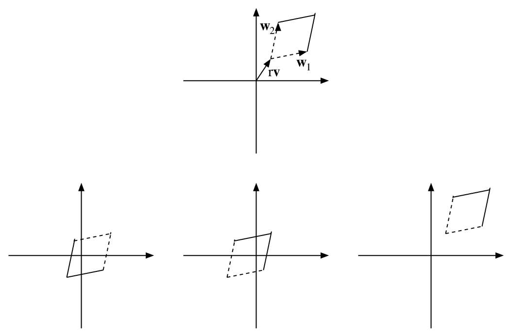
Now by the extended Brion-Theorem for simplices (Theorem 2.2) and the rational generating functions for simple cones,
∎
5. Concluding remarks
There exists a slightly more general version of our main Theorem 1.1. Namely, instead of one can take together with some facets of . Then on the other side of the reciprocity identity gets replaced by together with the remaining facets. This parallels a theorem of Stanley which generalizes Ehrhart-Macdonald Reciprocity [12].
There is also a theorem analogous to Brion’s for polyhedra (not just polytopes). Our proof goes through in this case once one allows unbounded simplices, which result when one moves a certain face of a simplex to infinity. (Any polyhedron can be triangulated into bounded and unbounded simplices.)
References
- [1] A. I. Barvinok, A polynomial time algorithm for counting integral points in polyhedra when the dimension is fixed, Math. Oper. Res. 19 (1994), 769–779.
- [2] M. Beck, S. Robins, F. Sottile, and J. Weitsman, Conic decompositions of polytopes, Preprint (2004).
- [3] C. J. Brianchon, Théorème nouveau sur les polyèdres, J. Ecole (Royale) Polytechnique 15 (1837), 317–319.
- [4] M. Brion, Points entiers dans les polyèdres convexes, Ann. Sci. École Norm. Sup. (4) 21 (1988), no. 4, 653–663.
- [5] E. Ehrhart, Sur les polyèdres rationnels homothétiques à dimensions, C. R. Acad. Sci. Paris 254 (1962), 616–618.
- [6] by same author, Sur un problème de géométrie diophantienne linéaire. I. Polyèdres et réseaux, J. Reine Angew. Math. 226 (1967), 1–29.
- [7] J. P. Gram, Om rumvinklerne i et polyeder, Tidsskrift for Math. (Copenhagen) 4 (1874), no. 3, 161–163.
- [8] H. Groemer, On the extension of additive functionals on classes of convex sets, Pacific J. Math. 75 (1978), no. 2, 397–410.
- [9] M.-N. Ishida, Polyhedral Laurent series and Brion’s equalities, Internat. J. Math. 1 (1990), no. 3, 251–265.
- [10] J. Lawrence, Rational-function-valued valuations on polyhedra, Discrete and computational geometry (New Brunswick, NJ, 1989/1990), Amer. Math. Soc., Providence, RI, 1991, pp. 199–208.
- [11] I. G. Macdonald, Polynomials associated with finite cell-complexes, J. London Math. Soc. (2) 4 (1971), 181–192.
- [12] R. P. Stanley, Combinatorial reciprocity theorems, Advances in Math. 14 (1974), 194–253.
- [13] by same author, Enumerative Combinatorics, 2nd ed., vol. I, Cambridge University Press, 1997.
- [14] W. Volland, Ein Fortsetzungssatz für additive Eipolyederfunktionale im euklidischen Raum, Arch. Math. 8 (1957), 144–149.