On the homology of the space of knots*Partially supported by the NSF Grant No. DMS-0072173 and CNRS-NSF Grant No. 17149

The purpose of this paper is to give homological properties of the classical spaces of smooth ‘long’ embeddings ${\mathcal{K}}_{3,1}={\mathrm{Emb}}({\mathbb{R}},{\mathbb{R}}^{3})$ and smooth embeddings ${\mathrm{Emb}}(S^{1},S^{3})$. Some results here also apply to the embedding spaces ${\mathrm{Emb}}(S^{j},S^{n})$, and ‘long’ embedding spaces ${\mathcal{K}}_{n,j}={\mathrm{Emb}}({\mathbb{R}}^{j},{\mathbb{R}}^{n})$, with the main results focused on the $3$-dimensional case $j=1$, $n=3$.

The approach here to these homological problems follows recent work of Hatcher [23, 24] and Budney [5, 7]. The homotopy type of the components of ${\mathrm{Emb}}(S^{1},S^{3})$ and ${\mathcal{K}}_{3,1}$ are understood completely in terms of configuration spaces in the plane, Stiefel manifolds, isometry groups of certain hyperbolic link complements and various natural iterated bundle operations. Many of the homological properties of both ${\mathcal{K}}_{3,1}$, and ${\mathrm{Emb}}(S^{1},S^{3})$ follow from combining this information together with earlier work of Cohen [12] on configuration spaces.

The space ${\mathcal{K}}_{n,1}$ admits the structure of an $H$-space induced by concatenation of ‘long’ embeddings. In addition, this $H$-space structure for ${\mathcal{K}}_{3,1}$ was shown to extend to a free ${\mathcal{C}}_{2}$-space in the sense of May, with “generating set” given by the space of prime long knots [5].

One consequence is that the homotopy type of the space of long knots is determined completely by the homotopy type of the prime long knots. Information concerning spaces of prime long knots is combined with bundle theoretic constructions to give a large contribution to the homology groups for spaces of long knots, as well as ${\mathrm{Emb}}(S^{1},S^{3})$.

The structure of a graded analogue of a Poisson algebra, a Poisson-Gerstenhaber algebra, arises in the work here. An introduction to Poisson algebras is given in [11], pages $177$-$182$ while some applications are given in [12] pages $215$-$216$ and [49]. A Poisson-Gerstenhaber algebra $A$ is a graded commutative algebra over $\mathbb{Q}$ given by $A_{n}$ in gradation $n$ together with a graded skew symmetric bilinear map

which satisfies the following where $|a|$ denotes the degree of an element $a$ in $A$:

1. 1.

   the Jacobi identity

   $$\{a,\{b,c\}\}=(-1)^{|a|+|b|+|c|+1}\{\{a,b\},c\}+(-1)^{|b||c|+|c|+1}\{\{a,c\},b\}$$

   where the signs will be typically omitted with the above written as

   $$\{\{a,\{b,c\}\}=(\pm 1)\{\{a,b\},c\}+(\pm 1)\{\{a,c\},b\}.$$

2. 2.

   the Leibniz formula

   $$\{a\cdot b,c\}=a\cdot\{b,c\}+(-1)^{|b||a|}b\{a,c\}.$$

A standard example of such a Gerstenhaber-Poisson algebra is given by the rational homology algebra of $\Omega^{2}(X)$ for $X$ a bouquet of spheres of dimension at least $3$ by [12] in which the precise axioms are recorded.

The mod-$p$ homology of ${\mathcal{K}}_{3,1}$ has more detailed structure, and is, loosely speaking, a ‘free restricted Gerstenhaber-Poisson algebra’ with additional structure satisfied by free $\mathcal{{\mathcal{C}}}_{2}$-spaces [12], freely generated on the mod-$p$ homology of the subspace of prime long knots.

The main results of the current article are Theorem 1.3 on the structure of the homology of ${\mathcal{K}}_{3,1}$, Proposition 1.4 concerning implications for the space of smooth embeddings of $S^{1}$ in $S^{3}$, Proposition 1.5, a homological characterization of the unknot, as well as Theorem 9.1 on the minimal $i$ such that $H_{i}({\mathcal{K}}_{3,1};{\mathbb{Z}})$ contains $p$-torsion.

Let $X_{{\mathcal{K}}}=\{f\in{\mathcal{K}}_{3,1}:f\text{ is prime}\}$, where the word ‘prime’ is used in the traditional sense of Schubert [43], that is $X_{{\mathcal{K}}}$ is the union of the connected components of ${\mathcal{K}}_{3,1}$ which contain knots that are not connected sums of two or more non-trivial knots, nor are they allowed to contain the unknot.

The above theorem can be thought of as a generalization of Schubert’s Theorem which states that $\pi_{0}{\mathcal{K}}_{3,1}$ is a free commutative monoid on countably-infinite many generators [43]. Schubert’s theorem is about the monoid structure on $\pi_{0}{\mathcal{K}}_{3,1}$ induced by the cubes action, while the above theorem is space-level on ${\mathcal{K}}_{3,1}$.

In general, ${\mathcal{K}}_{n,1}$ is a homotopy-associative $H$-space with multiplication induced by concatenation. This multiplication gives a product operation

Since ${\mathcal{K}}_{3,1}$ admits the action of the operad of little $2$-cubes, there is an induced map

together with an operation in homology with any coefficients

which is denoted, up to sign, by

for $\alpha$ in $H_{s}({\mathcal{K}}_{3,1})$, $\beta$ in $H_{t}({\mathcal{K}}_{3,1})$ and $\iota\in H_{1}(S^{1})$ the fundamental class. These operations satisfy the structure of a graded Poisson algebra for which the bracket operation $\lambda_{1}(\alpha,\beta)$ is called the Browder operation in [12].

The next result uses the product operation above as well as the bracket operation $\{\alpha,\beta\}=\lambda_{1}(\alpha,\beta)$, and follows by interweaving the results of 1.2, and [12]. We will use the notation ${\mathbb{F}}_{p}={\mathbb{Z}}/p{\mathbb{Z}}$ to denote the field with $p$ elements, when $p$ is a prime. To state these results, additional information given by three functors from graded vector spaces $V$ over a field ${\mathbb{F}}$ are described next with complete details given in Section 5:

1. 1.

   If the characteristic of the field is $0$ then the value of the functor on objects $V$ is the symmetric algebra generated by an algebraically ‘desuspended’ free Lie algebra generated by the suspension of $V$, and denoted

   $$S[\sigma^{-1}L[\sigma(V)]].$$

   This last algebra is a free Gerstenhaber-Poisson algebra.

2. 2.

   For the field ${\mathbb{F}}_{2}$ the value of the functor on objects $V$ is the symmetric algebra generated by an algebraically ‘desuspended’ free, mod-$2$ restricted Lie algebra generated by the suspension of $V$, and denoted

   $$S[\sigma^{-1}L^{(2)}[\sigma(V)]].$$

   This last algebra is a graded version of a free restricted Lie algebra.

3. 3.

   For the field ${\mathbb{F}}_{p}$ ($p$ an odd prime), then the value of the functor on objects $V$ is the symmetric algebra generated by an algebraically “desuspended” mod-$p$ free restricted Lie algebra generated by the suspension of $V$ plus an additional summand as described in Section 5, and denoted

   $$S[\sigma^{-1}L^{(p)}[\sigma(V)]\oplus\sigma^{-2}W^{p}[\sigma(V)]].$$

A primary development in this paper is our recursive application of the above theorem. Let $K_{c}\subset{\mathcal{K}}_{3,1}$ denote the subspace of ${\mathcal{K}}_{3,1}$ consisting of all cable knots. There is a homotopy-equivalence ${\mathbb{Z}}\times S^{1}\times{\mathcal{K}}_{3,1}\to K_{c}$. Let $K_{s}\subset{\mathcal{K}}_{3,1}$ denote the subspace of ${\mathcal{K}}_{3,1}$ which are connect-sums of any number of cable knots. Then there is a homotopy-equivalence ${\mathcal{C}}_{2}(K_{c}\sqcup\{*\})\to K_{s}$. The composite of the two maps is a homotopy-equivalence ${\mathcal{C}}_{2}(({\mathbb{Z}}\times S^{1}\times{\mathcal{K}}_{3,1})\sqcup\{*\})\to K_{s}$. Since $K_{s}$ is a collection of path-components of ${\mathcal{K}}_{3,1}$, this map can be iterated, giving a the homology of ${\mathcal{K}}_{3,1}$, as a Gerstenhaber-Poisson algebra, a fractal-like structure. These statements will be justified in Sections 2 and 3, and explored more fully in Sections 7 and 10.

These results lead to some natural questions about the structure of the homology of the higher-dimensional embedding spaces ${\mathcal{K}}_{n,1}$ ($n\geq 4$) studied recently by Sinha [45], Volic [51], Lambrechts [32] as well as others [1, 10, 17, 30, 41]. Constructions related to these questions are also addressed here.

By Theorem 1.3, there is arbitrarily large $p$-torsion in the homology of ${\mathcal{K}}_{3,1}$. Examples of Theorem 1.3 for knots whose path-components have higher $2$-torsion in their integer homology is given next. This higher torsion can be regarded as a coarse “measure” of the “complexity” of a knot’s JSJ-decomposition.

1. 1.

   Let ${\mathcal{K}}_{3,1}(f)$ denote the path-component of a torus knot $f$. Thus ${\mathcal{K}}_{3,1}(f)$ has the homotopy type of a circle [24, 7].

2. 2.

   Given any space $X$, and a strictly positive integer $q$, define

   $$E(q,X)={\mathrm{Conf}}({\mathbb{R}}^{2},q)\times_{\Sigma_{q}}X^{q}.$$

   Assume that ${\mathcal{K}}_{3,1}(f)$ has the homotopy type of $S^{1}$. $E(4,{\mathcal{K}}_{3,1}(f))$ has the property that

   1. (a)

      $H_{2}(E(4,{\mathcal{K}}_{3,1}(f)))={{\mathbb{Z}}/2{\mathbb{Z}}}$,

   2. (b)

      $H_{3}(E(4,{\mathcal{K}}_{3,1}(f)))=0$,

   3. (c)

      $H_{3}(S^{1}\times E(4,{\mathcal{K}}_{3,1}(f)))$ is isomorphic to ${{\mathbb{Z}}/2{\mathbb{Z}}}$.

   4. (d)

      Furthermore, $E(2^{s},S^{1}\times E(4,{\mathcal{K}}_{3,1}(f)))$ has the homotopy type of a path-component ${\mathcal{K}}_{3,1}(g)$ for a long knot $g$ as given in [5], and has torsion of order $2^{s+1}$ in its integer homology by Section 6, and 7. In this case, $g$ is a connected-sum of $2^{s}$ copies of the same summand, and that summand is a $p/q$-cable of a connected sum of four copies of the same torus knot. In the language of [6],

      $$g=\left(\left(T^{(p,q)}{\Delta}_{4}{\bowtie}{\mathcal{H}}^{4}\right){\bowtie}{\mathcal{S}}^{(p,q)}\right){\Delta}_{2^{s}}{\bowtie}{\mathcal{H}}^{2^{s}}$$

      The elements of this notation is described in detail in [6] and is summarized in Section 2.

   5. (e)

      A second example is $E(2^{s},{\mathcal{K}}_{3,1}(h)))$ where $h=T^{(p,q)}{\bowtie}W$ and $W$ is the Whitehead link. In this case,

      $${\mathcal{K}}_{3,1}(h)\simeq S^{1}\times\left(S^{1}\times_{\Sigma_{2}}S^{1}\right)$$

      where $S^{1}\times_{\Sigma_{2}}S^{1}$ is the Klein bottle [7]. $H_{1}({\mathcal{K}}_{3,1}(h)))={{\mathbb{Z}}/2{\mathbb{Z}}}\oplus{\mathbb{Z}}^{2}$.

A more complete description of the homology of ${\mathcal{K}}_{3,1}$ is given in Sections 5, and 6. The homology of each path-component is given in terms of Theorem 1.3 as well as filtrations of the values of the functors listed in that theorem.

Consider the subspace $\mathcal{T}{\mathcal{K}}_{3,1}$ of ${\mathcal{K}}_{3,1}$ consisting of the union of the components of ${\mathcal{K}}_{3,1}$ corresponding to knots which can be obtained from torus knots via iterations of the operations given by cabling and connected-sum. These are the knots whose complements are ‘graph manifolds’ ie: a union of Seifert-fibered manifolds. The structure of the homology of $\mathcal{T}{\mathcal{K}}_{3,1}$ is described in Section 10. This is our primary source of $p^{n}$-torsion in $H_{*}({\mathcal{K}}_{3,1};{\mathbb{Z}})$.

A further consequence of Theorem 1.2 is the next result which follows directly, and is proven in Section 4. Let ${\mathrm{Emb}}_{*}(S^{1},S^{n})$ denote the space of smooth pointed embeddings.

Section 4 gives precise relationships (such as the above proposition) between the homotopy-type of the embedding spaces ${\mathcal{K}}_{n,j}$, ${\mathrm{Emb}}(S^{j},S^{n})$ and ${\mathrm{Emb}}(S^{j},{\mathbb{R}}^{n})$.

Notice that the homological properties of each path component thus give knot invariants. This is illustrated by the following proposition.

In addition, a characterization of the components of ${\mathcal{K}}_{3,1}$ such that $H_{1}({\mathcal{K}}_{3,1}(f);{\mathbb{Z}})$ contains $2$-torsion is given in Section 8. A precise identification of those knots $f$ such that $H_{1}({\mathcal{K}}_{3,1}(f);{\mathbb{Z}})$ contains a ${{\mathbb{Z}}/2{\mathbb{Z}}}$ summand is also given. In Section 9 the least degree in which odd $p$ torsion in $H_{*}({\mathcal{K}}_{3,1};{\mathbb{Z}})$ occurs is as follow.

Much recent progress has been made on the structure of spaces of embeddings via finite-dimensional model spaces and approximations. Some of this was first given by Vassiliev [50] and has been the subject of further study via the Goodwillie Calculus of Embeddings by Sinha [45], Volic [51] Lambrechts [32], or cohomological techniques such as Bott-Taubes integrals [4, 10].

The Gerstenhaber-Poisson algebra above was first considered on the $E^{2}$-level of the Vassiliev spectral sequence by Tourtchine [49]. Related progress is given in work of Altshuler-Freidel [1], Bar-Natan [2], Cattaneo, Cotta-Ramusino-Longoni [10], Kohno [30], Kontsevich [31], Lescop [33], Polyak-Viro [40], Sakai [41], Watanabe [52] as well as others.

This paper takes the direction of using Gramain and Hatcher’s techniques for understanding the homotopy type of ${\mathcal{K}}_{3,1}$, one component at a time [18, 24]. The central construction of Hatcher [24] is to consider the components of the knot space as the classifying space of the mapping class group of the knot complement. One then studies how such a mapping class group acts on the JSJ-tree of the knot complement as in [5, 7], using Hatcher’s results on the homotopy type of diffeomorphism groups of Haken manifolds [21] to assemble an answer. Thus most of the results here are complementary to the results of the authors mentioned in the previous two paragraphs.

The authors would like to thank the University of Tokyo, the Max Planck Institute for Mathematics in Bonn, Institut des Hautes Études Scientifiques, the Institute for Advanced Study, the Pacific Institute of Mathematics and the American Institute of Mathematics for partial support during the preparation of this paper.

TABLE OF CONTENTS

1

Introduction

2

Notation, labelling components

3

The homotopy type of ${\mathcal{K}}_{3,1}$

4

Relations among various spaces

5

On the homology of ${\mathcal{C}}_{2}(X\amalg\{*\})$

6

On the homology of ${\mathcal{K}}_{3,1}$

7

Higher $p$-torsion in the integer homology of ${\mathcal{K}}_{3,1}$

8

$H_{1}({\mathcal{K}}_{3,1};{\mathbb{Z}})$

9

The first appearance of odd $p$-torsion

10

On the subspace generated by torus knots

11

Closed knots and homology

12

Problems

Whitney [56] showed that the embedding space ${\mathcal{K}}_{n,j}$ is connected for $n>2j+1$. By work of Wu [53], ${\mathcal{K}}_{n,j}$ is also connected provided both $n>2j\text{ and }j>1$. That ${\mathcal{K}}_{n,1}$ is also connected for $n=1$ is elementary. The fact that ${\mathcal{K}}_{2,1}$ is connected is equivalent to the smooth Alexander/Schoenflies theorem in dimension 2. In co-dimension $3$ and higher. Haefliger [20] vastly generalized Whitney’s result, proving that ${\mathcal{K}}_{n,j}$ is connected provided $2n>3j+3$, and $\pi_{0}{\mathcal{K}}_{n,j}$ is non-trivial for $2n=3j+3$. This work has recently been extended by the first author to a computation of the first non-trivial homotopy group of ${\mathcal{K}}_{n,j}$ provided $2n-3j-3\geq 0$ [8].

When $2n\leq 3j+3$ the space ${\mathcal{K}}_{n,j}$ could potentially have many connected components. $\pi_{0}{\mathcal{K}}_{n,j}$ was shown to be a group by Haefliger [20] provided $n-j>2$, whereas it is only a monoid for $n-j\leq 2$. A fundamental example is the space ${\mathcal{K}}_{3,1}$ which has countably infinite many components, and no inverses in the monoid $\pi_{0}{\mathcal{K}}_{3,1}$ [44]. Given $f\in{\mathcal{K}}_{n,j}$, let ${\mathcal{K}}_{n,j}(f)$ denote the path-component of ${\mathcal{K}}_{n,j}$ containing $f$.

We will use the notation ${\mathrm{EC}({1,D^{n-1}})}$ as defined in [5] for the space of framed long knots in ${\mathbb{R}}^{n}$. Given a compact manifold $M$, define

Here the support of $f$, $supp(f)$ is defined by $supp(f)=\{x\in{\mathbb{R}}^{k}\times M:f(x)\neq x\}$ and ${\mathsf{I}}=[-1,1]$. ${\mathrm{EC}({1,D^{n-1}})}$ is not homotopy equivalent to ${\mathcal{K}}_{n,1}$ in general, but as described in [5] there is a fibration

which splits at the fibre (via a $2$-cubes map) for $n\in\{1,2,3\}$, allowing us to think of ${\mathcal{K}}_{3,1}$ as a sub $2$-cubes object of ${\mathrm{EC}({1,D^{2}})}$.

This section collects information on the indexing of the components of ${\mathcal{K}}_{3,1}$ which is given in terms of the ‘companionship tree’ classification of knots, an application of the Jaco-Shalen-Johannson (JSJ) decomposition of knot complements. The indexing that we will use is described in detail in [6]. Aspects of this indexing have been partially described before in the works of Budney [5], Eisenbud and Neumann [14], Schubert [44], and the unpublished work of Bonahon and Siebenmann [3], as well as the survey work of Kawauchi [28]. Indeed, the results in [6] should be thought of as a uniqueness statement for Schubert’s satellite operations that he describes in [44]. In the book by Eisenbud-Neumann [14] this method of indexing is called the splice decomposition of links, but is specialized to the case of links in homology spheres whose complements are graph manifolds. A terse statement of the results in [6] given next suffice for the applications here. More complete as well as more specific information is given in [6].

The role of splicing is that it is an operation that takes knots and $KGL$’s as input and produces a knot of greater ‘complexity’ in the sense that the companionship trees of the input data is spliced together to produce the companionship tree of $J{\bowtie}L$. We proceed to make these ideas more precise.

Unlike links with Seifert-fibred complements, hyperbolic KGLs have no known canonical enumeration.

Some elementary examples of hyperbolic KGLs are:

• •

  the figure-8 knot

• •

  the Whitehead link

• •

  the Borromean rings

Hyperbolic KGLs of arbitrarily many components are known to exist by the work of Kanenobu [27]. For details on the hyperbolic structures, see for example the textbook of Thurston [48].

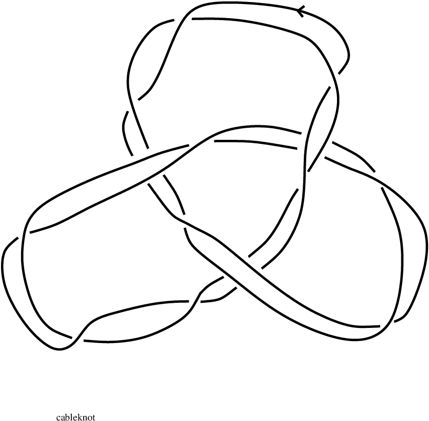
Figures 4 and 5 give examples of knots $K$ and the associated tree ${\mathbb{G}}_{K}$, and the corresponding splice notation, where $F_{8}$ denotes the figure-8 knot. Let $B=(B_{0},B_{1},B_{2})$ denote the Borromean rings, and let $B_{i,j}$ be the $3$-component link in $S^{3}$ obtained from $B$ by doing $i$ Dehn twists about the spanning disc of $B_{1}$ and $j$ Dehn twists about the spanning disc for $B_{2}$.

The spaces ${\mathrm{EC}({1,D^{n-1}})}$ admit an action of the operad of little $2$-cubes [5]. Using the connectedness of ${\mathcal{K}}_{n,1}$ for $n\geq 4$ together with the cubes action one can prove that ${\mathrm{EC}({1,D^{n-1}})}$ has the homotopy type of a $2$-fold loop space for $n\geq 4$. At present it is not known what the 2-fold de-looping of ${\mathrm{EC}({1,D^{n-1}})}$ is. Recently, P. Salvatore [42] has constructed an action of the operad of $2$-cubes on ${\mathcal{K}}_{n,1}$ for all $n\geq 4$.

The previously described fibre bundle

whose fibre inclusion $i:{\mathcal{K}}_{3,1}\to{\mathrm{Emb}}(S^{1},S^{3})$ is induced by the one-point compactification is explored more deeply in Section 4. For the purpose of this section and the study of the components of ${\mathcal{K}}_{3,1}$ and ${\mathrm{Emb}}(S^{1},S^{3})$ respectively, we note that the inclusion ${\mathcal{K}}_{3,1}\to{\mathrm{Emb}}(S^{1},S^{3})$ induces bijection on path-components. Thus, our indexing of $\pi_{0}{\mathrm{Emb}}(S^{1},S^{3})$ above by companionship trees ${\mathbb{G}}_{K}$ is also an indexing of $\pi_{0}{\mathcal{K}}_{3,1}$.

A detailed description of the homotopy type of ${\mathcal{K}}_{3,1}$ is given in this section. This description is given in terms of the splicing operations as described in Section 2. A good general reference for these results is the work [7].

1. 1.

   If $f$ is the unknot then ${\mathcal{K}}_{3,1}(f)$ is contractible by work of Hatcher [24].

2. 2.

   If $f$ is a $p/q$-cabling of $g$ then by work of Hatcher [24], there is a homotopy equivalence

   $$S^{1}\times{\mathcal{K}}_{3,1}(g)\to{\mathcal{K}}_{3,1}(f).$$

   We consider a torus knot to be a cable of the unknot, so we are claiming all non-trivial torus knots $f$ satisfy ${\mathcal{K}}_{3,1}(f)\simeq S^{1}$.

3. 3.

   If $f=(f_{1},f_{2},\cdots,f_{n}){\bowtie}{\mathcal{H}}^{n}$ where $\{f_{i}:i\in\{1,2,\cdots,n\}\}$ are the prime summands of $f$ and $n\geq 2$, then there is a homotopy equivalence

   $${\mathcal{C}}_{2}(n)\times_{\Sigma_{f}}\prod_{i=1}^{n}{\mathcal{K}}_{3,1}({f_{i}})\to{\mathcal{K}}_{3,1}(f)$$

   where $\Sigma_{f}\subset\Sigma_{n}$ is the Young subgroup corresponding to the partition $\sim$ of $\{1,2,\cdots,n\}$ given by $i\sim j\Leftrightarrow{\mathcal{K}}_{3,1}(f_{i})={\mathcal{K}}_{3,1}(f_{j})$. This result originally appears in [5].

4. 4.

   If a knot $f=(f_{1},f_{2},\cdots,f_{n}){\bowtie}L$ where $L$ is a hyperbolic KGL then there is a homotopy-equivalence:

   $$S^{1}\times\left(SO(2)\times_{A_{f}}\prod_{i=1}^{n}{\mathcal{K}}_{3,1}(f_{i})\right)\to{\mathcal{K}}_{3,1}(f).$$

   we define $A_{f}$ as a subgroup of $B_{L}$. $B_{L}$ is the subgroup of the group of hyperbolic isometries of the complement of $L$ in $S^{3}$ which:

   • •

     extend to diffeomorphisms of $S^{3}$.

   • •

     the extensions preserve $L_{0}$ and its orientation (ie: they act on the cusp corresponding to $L_{0}$ by translations).

   • •

     put together, the above two properties imply there is an embedding $B_{L}\to{\mathrm{Diff}}(S^{3};L,L_{0})$.

   It is a non-trivial fact [7] that the composite is an embedding of groups $B_{L}\to{\mathrm{Diff}}(S^{3};L,L_{0})\to{\mathrm{Diff}}^{+}(L_{0})$ where ${\mathrm{Diff}}^{+}(L_{0})$ is the group of orientation-preserving diffeomorphisms of $L_{0}$. Regard $B_{L}$ as a finite subgroup of $SO(2)$. There is a representation of $B_{L}$ given by the composite: $B_{L}\to{\mathrm{Diff}}(S^{3},L,L_{0})\to{\mathrm{Diff}}(\sqcup_{i=1}^{n}L_{i})\to\pi_{0}{\mathrm{Diff}}(\sqcup_{i=1}^{n}L_{i})\equiv\Sigma_{n}^{+}$ where we identify $\pi_{0}{\mathrm{Diff}}(\sqcup_{i=1}^{n}L_{i})$ with $\Sigma^{+}_{n}$, the signed symmetric group on $\{1,2,\cdots,n\}$. $\Sigma_{n}$ acts on ${\mathcal{K}}_{3,1}^{n}$ by permutation of factors. $\Sigma_{2}$ acts on ${\mathcal{K}}_{3,1}$ by knot inversion – fix an axis perpendicular to the long axis, and rotate a knot by $\pi$ about this axis, this is knot inversion. Stated another way, the group of rotations which preserve the long axis, $O(2)\subset SO(3)$, acts on ${\mathcal{K}}_{3,1}$ by conjugation. Fix an element $\varpi\in O(2)\setminus SO(2)$, then $\varpi$ acts as an involution on ${\mathcal{K}}_{3,1}$, thus defining an action of $\Sigma_{2}$ on ${\mathcal{K}}_{3,1}$. These two actions extend to an action of $\Sigma_{n}^{+}$ on ${\mathcal{K}}_{3,1}^{n}$. $A_{f}$ is the subgroup of $B_{L}$ that preserves the path-component $\prod_{i=1}^{n}{\mathcal{K}}_{3,1}(f_{i})$ of ${\mathcal{K}}_{3,1}^{n}$.

As mentioned in part (4) above, ${\mathcal{K}}_{3,1}$ is naturally an $O(2)$-space. Parts (1), (2) and (3) above all are $O(2)$-equivariant homotopy equivalences, as shown in [7]. Case (4) is only an $SO(2)$-equivariant homotopy-equivalence, although the homotopy-class of $\varpi$ acting on ${\mathcal{K}}_{3,1}$ is computed.

The goal of this section is to compare the homotopy types of the spaces:

• •

  ${\mathcal{K}}_{n,1}$

• •

  ${\mathrm{Emb}}(S^{1},S^{n})$

• •

  ${\mathrm{Emb}}(S^{1},{\mathbb{R}}^{n})$

The space of pointed, smooth embeddings ${\mathrm{Emb}}_{*}(S^{1},S^{n})$ will be a useful auxiliary space. Relationships between the embedding spaces ${\mathcal{K}}_{n,j}$, ${\mathrm{Emb}}(S^{j},S^{n})$ and ${\mathrm{Emb}}(S^{j},{\mathbb{R}}^{n})$ will also be listed.

References

- [1] D. Altshuler and L. Freidel, On universal Vassiliev invariants, Comm. Math. Phys., 170 (1995), 41–62.
- [2] D. Bar-Natan, On the Vassiliev knot invariants, Topology, 34(1995), 423–472.
- [3] F. Bonahon, L. Siebenmann, Geometric splittings of knots and Conway’s algebraic knots, unpublished preprint (1987).
- [4] R. Bott and C. Taubes, On the self-linking of knots, J. Math. Phys., 35(1994), 5247-5287.
- [5] R. Budney, Little cubes and long knots, Topology 46 (2007), 1–27. arXiv [math.GT/0309427]
- [6] R. Budney, JSJ-decompositions of knot complements in , l’Enseignement Mathématique (2) 52 (2006) 319–259. arXiv [math.GT/0506523]
- [7] R. Budney, The topology of knotspaces in dimension , arXiv [math.GT/0506523]
- [8] R. Budney, A family of embedding spaces, Geometry and Topology Monographs 13 (2007). arXiv [math.AT/0605069]
- [9] R. Budney, J. Conant, K. Scannell, D. Sinha, New perspectives on self-linking, Advances in Mathematics 191 (2005) 78–113.
- [10] A. Cattaneo, P. Cotta-Ramusino and R. Longoni, Configuration spaces and Vassiliev invariants in any dimension, Algebraic, and Geometric Topology, 2(2002), 949–1000.
- [11] V. Chari and A. Pressley, A Guide to Quantum Groups, Cambridge University Press, 1994.
- [12] F. R. Cohen, T. J. Lada and J. P. May, The homology of iterated loop spaces, Lecture Notes in Math., vol. 533. Springer-Verlag (1976).
- [13] C. Day, On link invariants of Vassiliev-type, Ph.D. thesis, University of North Carolina, 1993.
- [14] D. Eisenbud and W. Neumann, Three-dimensional link theory and invariants of plane curve singularities, Ann. Math. Stud. 110.
- [15] M. Falk, R. Randell, The lower central series of a fiber-type arrangement, Invent. Math., 82 (1985), 77–88.
- [16] E. Fadell and L. Neuwirth, Configuration spaces, Math. Scand., 10 (1962), 111-118.
- [17] T. Goodwillie, and M. Weiss, Embeddings from the point of view of immersion theory II, Geometric Topology, 3 (1999), 103-118.
- [18] A. Gramain, Sur le groupe fondamental de l’espace des noeuds, Ann. Inst. Fourier, Grenoble. 27,3 (1977), 29–44.
- [19] A. Haefliger, M. Hirsch, On the existence and classification of differentiable embeddings, Topology 2 (1963), 129–135.
- [20] A. Haefliger, Differentiable embeddings of in for , Ann. of Math., 2nd Ser. Vol 83 No. 3 (1966). 402–436.
- [21] A. Hatcher, Homeomorphisms of sufficiently-large -irreducible -manifolds, Topology, 15 (1976)
- [22] A. Hatcher, A proof of the Smale conjecture, Ann. of Math. 177 (1983)
- [23] A. Hatcher, Topological Moduli Spaces of Knots, Oct, 2002. Personal webpage at [http://www.math.cornell.edu/]
- [24] A. Hatcher, Spaces of Knots, arXiv [math.GT/9909095].
- [25] M. W. Hirsch, Differential topology, Graduate Texts in Mathematics, 33. Springer-Verlag, New York, 1976.
- [26] N. Jacobson, Lie Algebras, Interscience Tracts in Pure and Applied Mathematics, No. 10. Interscience Publishers (John Wiley & Sons), New York-London. 1962
- [27] T. Kanenobu, Hyperbolic links with Brunnian properties, J. Math. Soc. Japan. Vol. 38 No. 2, (1986) 295–308.
- [28] A. Kawauchi, A Survey of Knot Theory, Birkhauser Verlag. (1996)
- [29] T. Kohno, Vassiliev invariants and de Rham complex on the space of knots, Contemp. Math. 179(1994), 123-138.
- [30] T. Kohno, Loop spaces of configuration spaces and finite-type invariants, Geometry and Topology Monographs, Vol. 4. (2001) 143–160.
- [31] M. Kontsevich, Feynman diagrams and low diemensional topology, Progress in Mathematics, vol. , 1990, 120.
- [32] P. Lambrechts, V. Turchin, I. Volic, The rational homotopy type of spaces of knots in codimension , preprint.
- [33] C. Lescop, On configuration space integrals for links, Invariants of knots and 3-manifolds (Kyoto, 2001), 183–199 (electronic), Geom. Topol. Monogr., 4, Geom. Topol. Publ., Coventry, 2002.
- [34] G. I. Lehrer, The cohomology of a regular semisimple variety, J. Alg. 199(1998), 666-689.
- [35] G. I. Lehrer, G. B. Segal, Homology stability for classical semisimple varieties, Math. Zeit., 236 (2001) no. 2, 251–290.
- [36] S. Manfredini, Some subgroups of Artin’s braid group, Special issue on braid groups and related topics (Jerusalem, 1995). Topology Appl. 78 (1997), no. 1-2, 123-142.
- [37] J. P. May, The Geometry of Iterated Loop Spaces, Lect. Notes in Math., 268, Springer-Verlag, Berlin, 1972.
- [38] J. Milnor, J. Moore, On the structure of Hopf algebras, Ann. of Math., (2) 81 1965 211–264.
- [39] R. Palais, Local triviality of the restriction map for embeddings, Comment. Math. Helv. 34 (1960) 305–312.
- [40] M. Polyak, O. Viro, On the Casson knot invariant, Knots in Hellas ’98, vol. 3(Delphi). J. Knot Theory Ramifications, 10 (2001), no. 5, 711–738.
- [41] K. Sakai, Non-trivalent graph cocycle and cohomology of the long knot space, Algebraic & Geometric Topology 8(2008) 1499.1522.
- [42] P. Salvatore, Knots, operads and double loop spaces. IMRN (2006) arXiv [math.AT/0608490]
- [43] H. Schubert, Die eindeutige Zerlegbarkeit eines Knoten in Primknoten, Sitzungsber. Akad. Wiss. Heidelberg, math.-nat. KI., 3:57-167. (1949)
- [44] H. Schubert, Knoten und vollringe, Acta Mat. 90, 131–286 (1953)
- [45] D. Sinha, The topology of spaces of knots, arXiv [math.AT/0202287]
- [46] D. Sinha D. Sinha, Operads and knot spaces, J. Amer. Math. Soc. 19 (2006), no. 2, 461–486
- [47] D. Tamaki, A dual Rothenberg-Steenrod spectral sequence, Topology, 33(4)(1994), 631-662.
- [48] W. Thurston, Three-dimensional geometry and topology. Vol. 1. Edited by Silvio Levy. Princeton Mathematical Series, 35. Princeton University Press, Princeton, NJ, 1997. x+311 pp. ISBN: 0-691-08304-5
- [49] V. Tourtchine On the other side of the bialgebra of chord diagrams, J. Knot Thry. Ram. 16 (5) May 2007 575–629. arXiv.QA/0411436.
- [50] V. Vassiliev, Complements of discriminants of smooth maps: topology and applications, Translations of Mathematical Monographs, 98, American Mathematical Society, Providence, RI, 1992.
- [51] I. Volic, Finite-type knot invariants and calculus of functors, Compositio Mathematica 142 (2006) 222–250.
- [52] T. Watanabe, Configuration space integral for long n-knots, the Alexander polynomial and knot space cohomology, Algebraic and Geometric Topology 7 (2007) 47–92. arXiv [math.GT/0609742]
- [53] W. Wu, On the isotopy of -manifolds of dimension in euclidean -space. Sci. Record (N.S.) 2 (1958), 271–275.
- [54] H. Whitney, Topological properties of differentiable manifolds, Bull. Amer. Math. Soc., 43 (1937), 785–805.
- [55] H. Whitney, The self-intersections of a smooth -manifold in -space, Ann. of Math. (2) 45, 220–246 (1944).
- [56] H. Whitney, Differentiable Manifolds, Ann. of Math. (2) 37 (1936), 645–680.