The Full Scaling Limit of
Two-Dimensional Critical Percolation
Abstract
We use paths to construct a process of continuum nonsimple loops in the plane and prove that this process coincides with the full continuum scaling limit of 2D critical site percolation on the triangular lattice – that is, the scaling limit of the set of all interfaces between different clusters. Some properties of the loop process, including conformal invariance, are also proved. In the main body of the paper these results are proved while assuming, as argued by Schramm and Smirnov, that the percolation exploration path converges in distribution to the trace of chordal . Then, in a lengthy appendix, a detailed proof is provided for this convergence to , which itself relies on Smirnov’s result that crossing probabilities converge to Cardy’s formula.
Keywords: continuum scaling limit, percolation, SLE, critical behavior, triangular lattice, conformal invariance.
AMS 2000 Subject Classification: 82B27, 60K35, 82B43, 60D05, 30C35.
1 Introduction and Motivation
In the theory of critical phenomena it is usually assumed that a physical system near a continuous phase transition is characterized by a single length scale (the “correlation length”) in terms of which all other lengths should be measured. When combined with the experimental observation that the correlation length diverges at the phase transition, this simple but strong assumption, known as the scaling hypothesis, leads to the belief that at criticality the system has no characteristic length, and is therefore invariant under scale transformations. This suggests that all thermodynamic functions at criticality are homogeneous functions, and predicts the appearance of power laws. It also means that it should be possible to rescale a critical system appropriately and obtain a continuum model (the “continuum scaling limit”) which may have more symmetries and be easier to study than the original discrete model defined on a lattice.
Indeed, thanks to the work of Polyakov [23] and others [4, 5], it was understood by physicists since the early seventies that critical statistical mechanical models should possess continuum scaling limits with a global conformal invariance that goes beyond simple scale invariance, as long as the discrete models have “enough” rotation invariance. This property gives important information, enabling the determination of two- and three-point functions at criticality, when they are nonvanishing. Because the conformal group is in general a finite dimensional Lie group, the resulting constraints are limited in number; however, the situation becomes particularly interesting in two dimensions, since there every analytic function defines a conformal transformation, at least at points where . As a consequence, the conformal group in two dimensions is infinite-dimensional.
After this observation was made, a large number of critical problems in two dimensions were analyzed using conformal methods, which were applied, among others, to Ising and Potts models, Brownian motion, Self-Avoiding Walk (SAW), percolation, and Diffusion Limited Aggregation (DLA). The large body of knowledge and techniques that resulted, starting with the work of Belavin, Polyakov and Zamolodchikov [4, 5] in the early eighties, goes under the name of Conformal Field Theory (CFT). In two dimensions, one of the main goals of CFT and its most important application to statistical mechanics is a complete classification of all universality classes via irreducible representations of the infinite-dimensional Virasoro algebra.
Partly because of the success of CFT, work in recent years on critical phenomena seemed to slow down somewhat, probably due to the feeling that most of the leading problems had been resolved. Nonetheless, however powerful and successful it may be, CFT has some limitations and leaves various open problems. First of all, the theory deals primarily with correlation functions of local (or quasi-local) operators, and is therefore not always the best tool to investigate other quantities. Secondly, given some critical lattice model, there is no way, within the theory itself, of deciding to which CFT it corresponds. A third limitation, of a different nature, is due to the fact that the methods of CFT, although very powerful, are generally speaking not completely rigorous from a mathematical point of view.
In a somewhat surprising twist, the most recent developments in the area of two-dimensional critical phenomena have emerged in the mathematics literature and have followed a new direction, which has provided new tools and a way of coping with at least some of the limitations of CFT. The new approach may even provide a reinterpretation of CFT, and seems to be complementary to the traditional one in the sense that questions that are difficult to pose and/or answer within CFT are easy and natural in this new approach and vice versa.
The main tool of this radically new approach is the Stochastic Loewner Evolution (), or Schramm Loewner Evolution, as it is also known, introduced by Schramm [28]. The new approach, which is probabilistic in nature, focuses directly on non-local structures that characterize a given system, such as cluster boundaries in Ising, Potts and percolation models, or loops in the model. At criticality, these non-local objects become, in the continuum limit, random curves whose distributions can be uniquely identified thanks to their conformal invariance and a certain “Markovian” property. There is a one-parameter family of s, indexed by a positive real number , and they appear to be the only possible candidates for the scaling limits of interfaces of two-dimensional critical systems that are believed to be conformally invariant.
In particular, substantial progress has been made in recent years, thanks to , in understanding the fractal and conformally invariant nature of (the scaling limit of) large percolation clusters, which has attracted much attention and is of interest both for intrinsic reasons, given the many applications of percolation, and as a paradigm for the behavior of other systems. The work of Schramm [28] and Smirnov [30] has identified the scaling limit of a certain percolation interface with , providing, along with the work of Lawler-Schramm-Werner [19, 20] and Smirnov-Werner [34], a confirmation of many results in the physics literature, as well as some new results.
However, describes a single interface, which can be obtained by imposing special boundary conditions, and is not in itself sufficient to immediately describe the full scaling limit of the system. In fact, not only the nature and properties, but the very existence of the full scaling limit remained an open question. This is true of all models, such as Ising and Potts models, that are represented in terms of clusters. Werner [36] considered this problem in the context of for values of between and . For percolation (corresponding to ), the same problem was addressed in [7], where was used to construct a random process of continuous loops in the plane, which was identified with the full scaling limit of critical two-dimensional percolation, but without detailed proofs.
In this paper, we complete the analysis of [7], making rigorous the connection between the construction given there and the full scaling limit of percolation, and we prove some properties of the full scaling limit, the Continuum Nonsimple Loop process, including (one version of) conformal invariance. We do this in two parts. First, we give proofs in which we assume the validity of what we will call statement (S) (see Section 5), which is a specific version of the results of Schramm and of Smirnov [28, 30, 31, 32, 33] concerning convergence of percolation exploration paths to (see the discussion towards the end of Section 4.1). Since no detailed proof of statement (S) (or indeed, any version of convergence to ) has been available, in Appendix Appendix A: Convergence of the Percolation Exploration Path we give a proof based only on that part of Smirnov’s results about the convergence of crossing probabilities to Cardy’s formula [30] (see Theorem 4 in Appendix Appendix A: Convergence of the Percolation Exploration Path). We note that statement (S) is restricted to Jordan domains while no such restriction is indicated in [30, 31].
The rest of the paper is organized as follows. In Section 2, we give necessary definitions and introduce . Section 3 is devoted to the construction of the Continuum Nonsimple Loop process. In Section 4, we introduce the discrete model and a discrete construction analogous to the continuum one presented in Section 3. Most of the main results of this paper are stated in Section 5, while Section 6 contains the proofs of those results, which use (S). The long Appendix Appendix A: Convergence of the Percolation Exploration Path contains the proof of statement (S) (it is a consequence of Corollary A.1 there) and the short Appendix Appendix B: Sequences of Conformal Maps contains convergence results for sequences of conformal maps which are used throughout the paper.
We remark that although our proof in Appendix Appendix A: Convergence of the Percolation Exploration Path of convergence of exploration paths to roughly follows Smirnov’s outline [30, 31], based on his proof [30, 31] of convergence of crossing probabilities to Cardy’s formula and on the Markovian properties of hulls and tips, there are at least two technically significant modifications. The first is that we use a different sequence of stopping times to obtain a Markov chain approximation to , which results in a different geometry for the approximation (see Remark A.2). The second is that the control of “close encounters” by the exploration path to the domain boundary is not handled by general results for “three-arms” events at the boundary of a half-plane, but rather by an argument based on continuity of crossing probabilities with respect to domain boundaries (see Lemmas A.2, A.3, A.4 and A.5). Moreover, we cannot use directly Smirnov’s result on convergence of crossing probabilities (see Theorem 4), but need an extended version which is given in Theorem 6 of Appendix Appendix A: Convergence of the Percolation Exploration Path.
We conclude by noting that the convergence results of Appendix Appendix A: Convergence of the Percolation Exploration Path are sufficient not only for our purposes of obtaining the full scaling limit, but also for obtaining the critical exponents (see [34]).
2 Preliminary Definitions
We will find it convenient to identify the real plane and the complex plane . We will also refer to the Riemann sphere and the open upper half-plane (and its closure ), where chordal will be defined (see Section 2.3). will denote the open unit disc .
A domain of the complex plane is a nonempty, connected, open subset of ; a simply connected domain is said to be a Jordan domain if its (topological) boundary is a Jordan curve (i.e., a simple continuous loop).
We will make repeated use of Riemann’s mapping theorem, which states that if is any simply connected domain other than the entire plane and , then there is a unique conformal map of onto such that and .
2.1 Compactification of
When taking the scaling limit one can focus on fixed finite regions, , or consider the whole at once. The second option avoids dealing with boundary conditions, but requires an appropriate choice of metric.
A convenient way of dealing with the whole is to replace the Euclidean metric with a distance function defined on by
| (1) |
where the infimum is over all smooth curves joining with , parametrized by arclength , and where denotes the Euclidean norm. This metric is equivalent to the Euclidean metric in bounded regions, but it has the advantage of making precompact. Adding a single point at infinity yields the compact space which is isometric, via stereographic projection, to the two-dimensional sphere.
2.2 The Space of Curves
In dealing with the scaling limit we use the approach of Aizenman-Burchard [2]. Denote by the complete separable metric space of continuous curves in the closure of the disc of radius with the metric (2) defined below. Curves are regarded as equivalence classes of continuous functions from the unit interval to , modulo monotonic reparametrizations. will represent a particular curve and a parametrization of ; will represent a set of curves (more precisely, a closed subset of ). will denote the uniform metric on curves, defined by
| (2) |
where the infimum is over all choices of parametrizations of and from the interval . The distance between two closed sets of curves is defined by the induced Hausdorff metric as follows:
| (3) |
The space of closed subsets of (i.e., collections of curves in ) with the metric (3) is also a complete separable metric space. We denote by its Borel -algebra.
For each fixed , the random curves that we consider are polygonal paths on the edges of the hexagonal lattice , dual to the triangular lattice . A superscript is added to indicate that the curves correspond to a model with a “short distance cutoff” of magnitude .
We will also consider the complete separable metric space of continuous curves in with the distance
| (4) |
where the infimum is again over all choices of parametrizations of and from the interval . The distance between two closed sets of curves is again defined by the induced Hausdorff metric as follows:
| (5) |
The space of closed sets of (i.e., collections of curves in ) with the metric (5) is also a complete separable metric space. We denote by its Borel -algebra.
When we talk about convergence in distribution of random curves, we always mean with respect to the uniform metric (2), while when we deal with closed collections of curves, we always refer to the metric (3) or (5).
Remark 2.1.
In this paper, the space of closed sets of is generally used for collections of exploration paths and cluster boundary loops and their scaling limits, paths and continuum nonsimple loops. There is one place however, in the statements and proofs of Lemmas A.2, A.4 and A.5, where we also apply in essentially the original setting of Aizenman and Burchard [1, 2], i.e., for collections of blue and yellow simple -paths (see Section 4 for precise definitions) and their scaling limits. The slight modification needed to keep track of both the paths and their colors is easily managed.
2.3 Chordal in the Upper Half-Plane
The Stochastic Loewner Evolution () was introduced by Schramm [28] as a tool for studying the scaling limit of two-dimensional discrete (defined on a lattice) probabilistic models whose scaling limits are expected to be conformally invariant. In this section we define the chordal version of ; for more on the subject, the interested reader can consult the original paper [28] as well as the fine reviews by Lawler [17], Kager and Nienhuis [14], and Werner [37], and Lawler’s book [18].
Let denote the upper half-plane. For a given continuous real function with , define, for each , the function as the solution to the ODE
| (6) |
with . This is well defined as long as , i.e., for all , where
| (7) |
Let and let be the unbounded component of ; it can be shown that is bounded and that is a conformal map from onto . For each , it is possible to write as
| (8) |
when . The family is called the Loewner chain associated to the driving function .
Definition 2.1.
Chordal is the Loewner chain that is obtained when the driving function is times a standard real-valued Brownian motion with .
For all , chordal is almost surely generated by a continuous random curve in the sense that, for all , is the unbounded connected component of ; is called the trace of chordal .
2.4 Chordal in an Arbitrary Simply Connected Domain
Let () be a simply connected domain whose boundary is a continuous curve. By Riemann’s mapping theorem, there are (many) conformal maps from the upper half-plane onto . In particular, given two distinct points (or more accurately, two distinct prime ends), there exists a conformal map from onto such that and . In fact, the choice of the points and on the boundary of only characterizes up to a multiplicative factor, since would also do.
Suppose that is a chordal in as defined above; we define chordal in from to as the image of the Loewner chain under . It is possible to show, using scaling properties of , that the law of is unchanged, up to a linear time-change, if we replace by . This makes it natural to consider as a process from to in , ignoring the role of .
We are interested in the case , for which is generated by a continuous, nonsimple, non-self-crossing curve with Hausdorff dimension . We will denote by the image of under and call it the trace of chordal in from to ; is a continuous nonsimple curve inside from to , and it can be given a parametrization such that and , so that we are in the metric framework described in Section 2.2. It will be convenient to think of as an oriented path, with orientation from to .
3 Construction of the Continuum Nonsimple Loops
3.1 Construction of a Single Loop
As a preview to the full construction, we explain how to construct a single loop using two paths inside a domain whose boundary is assumed to have a given orientation (clockwise or counterclockwise). This is done in three steps (see Figure 1), of which the first consists in choosing two points and on the boundary of and “running” a chordal , , from to inside . As explained in Section 2.4, we consider as an oriented path, with orientation from to . The set is a countable union of its connected components, which are open and simply connected. If is a deterministic point in , then with probability one, is not touched by [26] and so it belongs to a unique domain in that we denote .
The elements of can be conveniently thought of in terms of how a point in the interior of the component was first “trapped” at some time by , perhaps together with either or (the portions of the boundary from to counterclockwise or clockwise respectively): (1) those components whose boundary contains a segment of between two successive visits at and to (where here and below ), (2) the analogous components with replaced by the other part of the boundary , (3) those components formed when with winding about in a counterclockwise direction between and , and finally (4) the analogous clockwise components.
We give to the boundary of a domain of type 3 or 4 the orientation induced by how the curve winds around the points inside that domain. For a domain of type 1 or 2 which is produced by an “excursion” from to , the part of the boundary that corresponds to the inner perimeter of the excursion (i.e., the perimeter of seen from ) is oriented according to the direction of , i.e., from to .
If we assume that is oriented from to clockwise, then the boundaries of domains of type 2 have a well defined orientation, while the boundaries of domains of type 1 do not, since they are composed of two parts which are both oriented from the beginning to the end of the excursion that produced the domain.
Now, let be a domain of type 1 and let and be respectively the starting and ending point of the excursion that generated . The second step to construct a loop is to run a chordal , , inside from to ; the third and final step consists in pasting together and .
Running inside from to partitions into new domains. Notice that if we assign an orientation to the boundaries of these domains according to the same rules used above, all of those boundaries have a well defined orientation, so that the construction of loops just presented can be iterated inside each one of these domains (as well as inside each of the domains of type 2, 3 and 4 generated by in the first step). This will be done in the next section.

3.2 The Full Construction Inside The Unit Disc
In this section we define the Continuum Nonsimple Loop process inside the unit disc via an inductive procedure. Later, in order to define the continuum nonsimple loops in the whole plane, the unit disc will be replaced by a growing sequence of large discs, , with (see Theorem 2). The basic ingredient in the algorithmic construction, given in the previous section, consists of a chordal path between two points and of the boundary of a given simply connected domain .
We will organize the inductive procedure in steps, each one corresponding to one inside a certain domain generated by the previous steps. To do that, we need to order the domains present at the end of each step, so as to choose the one to use in the next step. For this purpose, we introduce a deterministic countable set of points that are dense in and are endowed with a deterministic order (here and below by deterministic we mean that they are assigned before the beginning of the construction and are independent of the ’s).
The first step consists of an path, , inside from to , which produces many domains that are the connected components of the set . These domains can be priority-ordered according to the maximal - or - coordinate distances between points on their boundaries and using the rank of the points in (contained in the domains) to break ties, as follows. For a domain , let be the maximal - or -distance between points on its boundary, whichever is greater. Domains with larger have higher priority, and if two domains have the same , the one containing the highest ranking point of from those two domains has higher priority. The priority order of domains of course changes as the construction proceeds and new domains are formed.
The second step of the construction consists of an path, , that is produced in the domain with highest priority (after the first step). Since all the domains that are produced in the construction are Jordan domains, as explained in the discussion following Corollary 5.1, for all steps we can use the definition of chordal given in Section 2.4.
As a result of the construction, the paths are naturally ordered: . It will be shown (see especially the proof of Theorem 1 below) that every domain that is formed during the construction is eventually used (this is in fact one important requirement in deciding how to order the domains and therefore how to organize the construction).
So far we have not explained how to choose the starting and ending points of the paths on the boundaries of the domains. In order to do this, we give an orientation to the boundaries of the domains produced by the construction according to the rules explained in Section 3.1. We call monochromatic a boundary which gets, as a consequence of those rules, a well defined (clockwise or counterclockwise) orientation; the choice of this term will be clarified when we discuss the lattice version of the loop construction below. We will generally take our initial domain (or ) to have a monochromatic boundary (either clockwise or counterclockwise orientation).
It is easy to see by induction that the boundaries that are not monochromatic are composed of two “pieces” joined at two special points (call them A and B, as in the example of Section 3.1), such that one piece is a portion of the boundary of a previous domain, and the other is the inner perimeter of an excursion (see again Section 3.1). Both pieces are oriented in the same direction, say from A to B (see Figure 1).
For a domain whose boundary is not monochromatic, we make the “natural” choice of starting and ending points, corresponding to the end and beginning of the excursion that produced the domain (the points B and A respectively, in the example above). As explained in Section 3.1, when such a domain is used with this choice of points on the boundary, a loop is produced, together with other domains, whose boundaries are all monochromatic.
For a domain whose boundary is monochromatic, and therefore has a well defined orientation, there are various procedures which would yield the “correct” distribution for the resulting Continuum Nonsimple Loop process; one possibility is as follows.
Given a domain , and are chosen so that, of all pairs of points in , they maximize if , or else they maximize . If the choice is not unique, to restrict the number of pairs one looks at those pairs, among the ones already obtained, that maximize the other of . Notice that this leaves at most two pairs of points; if that’s the case, the pair that contains the point with minimal real (and, if necessary, imaginary) part is chosen. The iterative procedure produces a loop every time a domain whose boundary is not monochromatic is used. Our basic loop process consists of the collection of all loops generated by this inductive procedure (i.e., the limiting object obtained from the construction by letting the number of steps ), to which we add a “trivial” loop for each in , so that the collection of loops is closed in the appropriate sense [2]. The Continuum Nonsimple Loop process in the whole plane is introduced in Theorem 2, Section 5. There, a “trivial” loop for each has to be added to make the space of loops closed.
4 Lattices and Paths
We will denote by the two-dimensional triangular lattice, whose sites we think of as the elementary cells of a regular hexagonal lattice embedded in the plane as in Figure 2. A sequence of sites of such that and are neighbors in for all and whenever will be called a -path and denoted by . If the first and last sites of the path are neighbors in , the path will be called a -loop.
We say that a finite subset of is simply connected if both and are connected (by the edges of ). For a simply connected set of hexagons, we denote by its external site boundary, or s-boundary (i.e., the set of hexagons that do not belong to but are adjacent to hexagons in ), and by the topological boundary of when is considered as a domain of . We will call a bounded, simply connected subset of a Jordan set if its s-boundary is a -loop.
For a Jordan set , a vertex that belongs to can be either of two types, according to whether the edge incident on that is not in belongs to a hexagon in or not. We call a vertex of the second type an e-vertex (e for “external” or “exposed”).
Given a Jordan set and two e-vertices in , we denote by the portion of traversed counterclockwise from to , and call it the right boundary; the remaining part of the boundary is denote by and is called the left boundary. Analogously, the portion of of whose hexagons are adjacent to is called the right s-boundary and the remaining part the left s-boundary.

A percolation configuration on is an assignment of (equivalently, yellow) or (blue) to each site of . For a domain of the plane, the restriction to the subset of of the percolation configuration is denoted by . On the space of configurations , we consider the usual product topology and denote by the uniform measure, corresponding to Bernoulli percolation with equal density of yellow (minus) and blue (plus) hexagons, which is critical percolation in the case of the triangular lattice.
A (percolation) cluster is a maximal, connected, monochromatic subset of ; we will distinguish between blue (plus) and yellow (minus) clusters. The boundary of a cluster is the set of edges of that surround the cluster (i.e., its Peierls contour); it coincides with the topological boundary of considered as a domain of . The set of all boundaries is a collection of “nested” simple loops along the edges of .
Given a percolation configuration , we associate an arrow to each edge of belonging to the boundary of a cluster in such a way that the hexagon to the right of the edge with respect to the direction of the arrow is blue (plus). The set of all boundaries then becomes a collection of nested, oriented, simple loops. A boundary path (or b-path) is a sequence of distinct edges of belonging to the boundary of a cluster and such that and meet at a vertex of for all . To each b-path, we can associate a direction according to the direction of the edges in the path.
Given a b-path , we denote by (respectively, ) the set of blue (resp., yellow) hexagons (i.e., sites of ) adjacent to ; we also let .
4.1 The Percolation Exploration Process and Path
For a Jordan set and two e-vertices in , imagine coloring blue all the hexagons in and yellow all those in . Then, for any percolation configuration inside , there is a unique b-path from to which separates the blue cluster adjacent to from the yellow cluster adjacent to . We call a percolation exploration path (see Figure 3).
An exploration path can be decomposed into left excursions , i.e., maximal b-subpaths of that do not use edges of the left boundary . Successive left excursions are separated by portions of that contain only edges of the left boundary . Analogously, can be decomposed into right excursions, i.e., maximal b-subpaths of that do not use edges of the right boundary . Successive right excursions are separated by portions of that contain only edges of the right boundary .
Notice that the exploration path only depends on the percolation configuration inside and the positions of the e-vertices and ; in particular, it does not depend on the color of the hexagons in , since it is defined by imposing fictitious boundary conditions on . To see this more clearly, we next show how to construct the percolation exploration path dynamically, via the percolation exploration process defined below.
Given a Jordan set and two e-vertices in , assign to a counterclockwise orientation (i.e., from to ) and to a clockwise orientation. Call the edge incident on that does not belong to and orient it in the direction of ; this is the “starting edge” of an exploration procedure that will produce an oriented path inside along the edges of , together with two nonsimple monochromatic paths on . From , the process moves along the edges of hexagons in according to the rules below. At each step there are two possible edges (left or right edge with respect to the current direction of exploration) to choose from, both belonging to the same hexagon contained in or .
- •
If belongs to and has not been previously “explored,” its color is determined by flipping a fair coin and then the edge to the left (with respect to the direction in which the exploration is moving) is chosen if is blue (plus), or the edge to the right is chosen if is yellow (minus).
- •
If belongs to and has been previously explored, the color already assigned to it is used to choose an edge according to the rule above.
- •
If belongs to the right external boundary , the left edge is chosen.
- •
If belongs to the left external boundary , the right edge is chosen.
- •
The exploration process stops when it reaches .
We can assign an arrow to each edge in the path in such a way that the hexagon to the right of the edge with respect to the arrow is blue; for edges in , we assign the arrows according to the direction assigned to the boundary. In this way, we get an oriented path, whose shape and orientation depend solely on the color of the hexagons explored during the construction of the path.

When we present the discrete construction, we will encounter Jordan sets with two e-vertices assigned in some way to be discussed later. Such domains will have either monochromatic (plus or minus) boundaries or boundary conditions, corresponding to having both and monochromatic, but of different colors.
As explained, the exploration path does not depend on the color of , but the interpretation of does. For domains with boundary conditions, the exploration path represents the interface between the yellow cluster containing the yellow portion of the s-boundary of and the blue cluster containing its blue portion.
For domains with monochromatic blue (resp., yellow) boundary conditions, the exploration path represents portions of the boundaries of yellow (resp., blue) clusters touching and adjacent to blue (resp., yellow) hexagons that are the starting point of a blue (resp., yellow) path (possibly an empty path) that reaches , pasted together using portions of .
In order to study the continuum scaling limit of an exploration path, we introduce the following definitions.
Definition 4.1.
Given a bounded, simply connected domain of the plane, we denote by the largest Jordan set of hexagons of the scaled hexagonal lattice that is contained in , and call it the -approximation of .
It is clear that if is a Jordan domain, then as , converges to in the metric (2).
Definition 4.2.
Let be a bounded domain of the plane and its -approximation. For , choose the pair of e-vertices in closest to, respectively, and (if there are two such vertices closest to , we choose, say, the first one encountered going clockwise along , and analogously for ). Given a percolation configuration , we define the exploration path .
For a fixed , the measure on percolation configurations induces a measure on exploration paths . In the continuum scaling limit, , one is interested in the weak convergence of to a measure supported on continuous curves, with respect to the uniform metric (2) on continuous curves.
One of the main tools in this paper is the result on convergence to announced by Smirnov [30] (see also [31]), whose detailed proof is to appear [32]: The distribution of converges, as , to that of the trace of chordal inside from to , with respect to the uniform metric (2) on continuous curves.
Actually, we will rather use a slightly stronger conclusion, given as statement (S) at the beginning of Section 5 below, a version of which, according to [34] (see p. 734 there), and [33], will be contained in [32]. This stronger statement is that the convergence of the percolation process to takes place locally uniformly with respect to the shape of the domain and the positions of the starting and ending points and on its boundary . We will use this version of convergence to to identify the Continuum Nonsimple Loop process with the scaling limit of all critical percolation clusters. Statement (S) is a direct consequence of Corollary A.1, which is proved in Appendix Appendix A: Convergence of the Percolation Exploration Path. Although the convergence statements in Corollary A.1 and in (S) are stronger than those in [30, 31], we note that they are restricted to Jordan domains, a restriction not present in [30, 31].
Before concluding this section, we give one more definition. Consider the exploration path and the set . The set is the union of its connected components (in the lattice sense), which are simply connected. If the domain is large and the e-vertices are not too close to each other, then with high probability the exploration process inside will make large excursions into , so that will have more than one component. Given a point contained in , we will denote by the domain corresponding to the unique element of that contains (notice that for a deterministic , is well defined with high probability for small, i.e., when and ).
4.2 Discrete Loop Construction
Next, we show how to construct, by twice using the exploration process described in Section 4.1, a loop along the edges of corresponding to the external boundary of a monochromatic cluster contained in a large, simply connected, Jordan set with monochromatic blue (say) boundary conditions (see Figures 4 and 5).
Consider the exploration path and the sets and (see Figure 4). The set is the union of its connected components (in the lattice sense), which are simply connected. If the domain is large and the e-vertices are chosen not too close to each other, with large probability the exploration process inside will make large excursions into , so that will have many components.
There are four types of components which may be usefully thought of in terms of their external site boundaries: (1) those components whose site boundary contains both sites in and , (2) the analogous components with replaced by and by , (3) those components whose site boundary only contains sites in , and finally (4) the analogous components with replaced by .
Notice that the components of type 1 are the only ones with boundary conditions, while all other components have monochromatic s-boundaries. For a given component of type 1, we can identify the two edges that separate the yellow and blue portions of its s-boundary. The vertices and of where those two edges intersect are e-vertices and are chosen to be the starting and ending points of the exploration path inside .
If are respectively the ending and starting points of the left excursion of that “created” , by pasting together and with the help of the edges of contained between and and between and , we get a loop which corresponds to the boundary of a yellow cluster adjacent to (see Figure 5). Notice that the path in general splits into various other domains, all of which have monochromatic boundary conditions.


4.3 Full Discrete Construction
We now give the algorithmic construction for discrete percolation which is the analogue of the continuum one. Each step of the construction is a single percolation exploration process; the order of successive steps is organized as in the continuum construction detailed in Section 3.2. We start with the smallest Jordan set of hexagons that covers the unit disc . We will also make use of the countable set of points dense in that was introduced earlier.
The first step consists of an exploration process inside . For this, we need to select two points and in (which identify the starting and ending edges). We choose for the e-vertex closest to , and for the e-vertex closest to (if there are two such vertices closest to , we can choose, say, the one with smallest real part, and analogously for ). The first exploration produces a path and, for small, many new domains of all four types. These domains are ordered according to the maximal - or - distance between points on their boundaries and, if necessary, with the help of points in , as in the continuum case, and that order is used, at each step of the construction, to determine the next exploration process. With this choice, the exploration processes and paths are naturally ordered: .
Each exploration process of course requires choosing a starting and ending vertex and edge. For domains of type 1, with a or boundary condition, the choice is the natural one, explained before.
For a domain (used at the th step) of type other than 1, and therefore with a monochromatic boundary, the starting and ending edges are chosen with a procedure that mimics what is done in the continuum case. Once again, the exact procedure used to choose the pair of points is not important, as long as they are not chosen too close to each other. This is clear in the discrete case because the procedure that we are presenting is only “discovering” the cluster boundaries. In more precise terms, it is clear that one could couple the processes obtained with different rules by means of the same percolation configuration, thus obtaining exactly the same cluster boundaries.
As in the continuum case, we can choose the following procedure. (In Theorem 1 we will slightly reorganize the procedure by using a coupling to the continuum construction to guarantee that the order of exploration of domains of the discrete and continuum procedures match despite the rules for breaking ties.) Given a domain , and are chosen so that, of all pairs of points in , they maximize if , or else they maximize . If the choice is not unique, to restrict the number of pairs one looks at those pairs, among the ones already obtained, that maximize the other of . Notice that this leaves at most two pairs of points; if that’s the case, the pair that contains the point with minimal real (and, if necessary, imaginary) part is chosen.
The procedure continues iteratively, with regions that have monochromatic boundaries playing the role played in the first step by the unit disc. Every time a region with boundary conditions is used, a new loop, corresponding to the outer boundary contour of a cluster, is formed by pasting together, as explained in Section 3.1, the new exploration path and the excursion containing the region where the last exploration was carried out. All the new regions created at a step when a loop is formed have monochromatic boundary conditions.
5 Main Results
In this section we collect our main results about the Continuum Nonsimple Loop process. Before doing that, we state a precise version, called statement (S), on convergence of exploration paths to that we will use in the proofs of these results, presented in Section 6. (A proof of statement (S) is given in Appendix Appendix A: Convergence of the Percolation Exploration Path; it is an immediate consequence of Corollary A.1 there. The proof relies, among other things, on the result of Smirnov [30] concerning convergence of crossing probabilities to Cardy’s formula [10, 11] – see Theorem 4.) We note that (S) or (Corollary A.1) is both more general and more special than the convergence statements in [30, 31] — more general in that the domain can vary with as , but more special in the restriction to Jordan domains.
Given a Jordan domain with two distinct points on its boundary, let denote the law of , the trace of chordal , and let denote the law of the percolation exploration path . Let be the space of continuous curves inside from to . We define (where denotes the open ball of radius centered at in the metric (2)) and denote by the Prohorov distance; weak convergence is equivalent to convergence in the Prohorov metric. Statement (S) is the following; it is used in the proofs of all the results of this section except for Lemmas 5.1-5.2.
- (S)
For Jordan domains, there is convergence in distribution of the percolation exploration path to the trace of chordal that is locally uniform in the shape of the boundary with respect to the uniform metric on continuous curves (2), and in the location of the starting and ending points with respect to the Euclidean metric; i.e., for a Jordan domain with , , and such that for all with Jordan and with and , .
5.1 Preliminary Results
We first give some important results which are needed in the proofs of the main theorems. We start with two lemmas which are consequences of [2], of standard bounds on the probability of events corresponding to having a certain number of monochromatic crossings of an annulus (see Lemma 5 of [16] and Appendix A of [20]), but which do not depend on statement (S).
Lemma 5.1.
Let be the percolation exploration path on the edges of inside (the -approximation of) between (the e-vertices closest to) and . For any fixed point , chosen independently of , as , and the boundary of the domain that contains jointly have limits in distribution along subsequences of with respect to the uniform metric (2) on continuous curves. Moreover, any subsequence limit of is almost surely a simple loop [3].
Lemma 5.2.
Using the notation of Lemma 5.1, let be the limit in distribution of as along some convergent subsequence and the boundary of the domain of that contains . Then, as , converges in distribution to .
The two lemmas above are important ingredients in the proof of Theorem 1 below. The second one says that, for every subsequence limit, the discrete boundaries converge to the boundaries of the domains generated by the limiting continuous curve. If we use statement (S), then the limit of is the trace of chordal for every subsequence , and we can use Lemmas 5.2 and 5.1 to deduce that all the domains produced in the continuum construction are Jordan domains. The key step in that direction is represented by the following result, our proof of which relies on (S).
Corollary 5.1.
For any deterministic , the boundary of a domain of the continuum construction is almost surely a Jordan curve.
The corollary says that the domains that appear after the first step of the continuum construction are Jordan domains. The steps in the second stage of the continuum construction consist of paths inside Jordan domains, and therefore Corollary 5.1, combined with Riemann’s mapping theorem and the conformal invariance of , implies that the domains produced during the second stage are also Jordan. By induction, we deduce that all the domains produced in the continuum construction are Jordan domains.
We end this section with one more lemma which is another key ingredient in the proof of Theorem 1; we remark that its proof requires (S) in a fundamental way.
Lemma 5.3.
Let denote a random Jordan domain, with two points on . Let , be a sequence of random Jordan domains with points on their boundaries such that, as , converges in distribution to with respect to the uniform metric (2) on continuous curves, and the Euclidean metric on . For any sequence with as , converges in distribution to with respect to the uniform metric (2) on continuous curves.
5.2 The Main Theorems
In this section we state the main theorems of this paper and a corollary, our most important result, that the Continuum Nonsimple Loop process is the scaling limit of the set of all cluster boundaries for critical site percolation on the triangular lattice. The corollary is obtained by combining the first two theorems. The proofs of all these results rely on statement (S). As noted before, statement (S) is proved in Appendix Appendix A: Convergence of the Percolation Exploration Path.
Theorem 1.
For any , the first steps of (a suitably reorganized version of) the full discrete construction inside the unit disc (of Section 4.3) converge, jointly in distribution, to the first steps of the full continuum construction inside the unit disc (of Section 3.2). Furthermore, the scaling limit of the full (original or reorganized) discrete construction is the full continuum construction.
Moreover, if for any fixed we let denote the number of steps needed to find all the cluster boundaries of Euclidean diameter larger than in the discrete construction, then is bounded in probability as ; i.e., . This is so in both the original and reorganized versions of the discrete construction.
The second part of Theorem 1 means that both versions of the discrete construction used in the theorem find all large contours in a number of steps which does not diverge as . This, together with the first part of the same theorem, implies that the continuum construction does indeed describe all macroscopic contours contained inside the unit disc (with blue boundary conditions) as .
The construction presented in Section 3.2 can of course be repeated for the disc of radius , for any , so we should take a “thermodynamic limit” by letting . In this way, we would eliminate the boundary (and the boundary conditions) and obtain a process on the whole plane. Such an extension from the unit disc to the plane is contained in the next theorem.
Let be the (limiting) distribution of the set of curves (all continuum nonsimple loops) generated by the continuum construction inside (i.e., the limiting measure, defined by the inductive construction, on the complete separable metric space of collections of continuous curves in ).
For a domain , we denote by the mapping (on or ) in which all portions of curves that exit are removed. When applied to a configuration of loops in the plane, gives a set of curves which either start and end at points on or form closed loops completely contained in . Let be the same mapping lifted to the space of probability measures on or .
Theorem 2.
Theorem 1 implies that there exists a unique probability measure on the space of collections of continuous curves in such that as in the sense that for every bounded domain , as , .
Remark 5.1.
We remark that we will generally take monochromatic blue boundary conditions on the disc of radius . But one could also take monochromatic boundary conditions with color depending on or even non-monochromatic boundary conditions without any essential change in the results or the proofs.
Corollary 5.2.
The Continuum Nonsimple Loop process in the plane defined in Theorem 2 is the scaling limit of the collection of all boundary contours for critical site percolation on the triangular lattice.
The next theorem states some properties of the Continuum Nonsimple Loop process in the plane.
Theorem 3.
The Continuum Nonsimple Loop process in the plane has the following properties, the first three of which are valid with probability one:
- 1.
The Continuum Nonsimple Loop process is a random collection of noncrossing continuous loops in the plane. The loops can and do touch themselves and each other many times, but there are no triple points; i.e. no three or more loops can come together at the same point, and a single loop cannot touch the same point more than twice, nor can a loop touch a point where another loop touches itself.
- 2.
Any deterministic point (i.e., chosen independently of the loop process) of the plane is surrounded by an infinite family of nested loops with diameters going to both zero and infinity; any annulus about that point with inner radius and outer radius contains only a finite number of those loops. Consequently, any two distinct deterministic points of the plane are separated by loops winding around each of them.
- 3.
Any two loops are connected by a finite “path” of touching loops.
- 4.
The Continuum Nonsimple Loop process is conformally invariant in the sense that, given a Jordan domain and a conformal homeomorphism onto , the scaling limits, and , of the loops inside and taken with, say, blue boundary conditions are related by . (Here denotes the probability distribution of the loop process when is distributed by .)
To conclude this section, we show how to recover chordal from the Continuum Nonsimple Loop process, i.e., given a (deterministic) Jordan domain with two boundary points and , we give a construction that uses the continuum nonsimple loops of to generate a process distributed like chordal inside from to .
Remember, first of all, that each continuum nonsimple loop has either a clockwise or counterclockwise direction, with the set of all loops surrounding any deterministic point alternating in direction. For convenience, let us suppose that is at the “bottom” and is at the “top” of so that the boundary is divided into a left and right part by these two points. Fix and call the set of all the directed segments of loops that connect from the left to the right part of the boundary touching at a distance larger than from both and , and the analogous set of directed segments from the right to the left portion of . For a fixed , there is only a finite number of such segments, and, if they are ordered moving along the left boundary of from to , they alternate in direction (i.e., a segment in is followed by one in and so on).
Between a segment in and the next segment in , there are countably many portions of loops intersecting which start and end on and are maximal in the sense that they are not contained inside any other portion of loop of the same type; they all have counterclockwise direction and can be used to make a “bridge” between the right-to-left segment and the next one (in ). This is done by pasting the portions of loops together with the help of points in and a limit procedure to produce a connected (nonsimple) path.
If we do this for each pair of successive segments on both sides of the boundary of , we get a path that connects two points on . By letting and taking the limit of this procedure, since almost surely and are surrounded by an infinite family of nested loops with diameters going to zero, we obtain a path that connects with ; this path is distributed as chordal inside from to . The last claim follows from considering the analogous procedure for percolation on the discrete lattice , using segments of boundaries. It is easy to see that in the discrete case this procedure produces exactly the same path as the percolation exploration process. By Corollary 5.2, the scaling limit of this discrete procedure is the continuum one described above, therefore the claim follows from (S).
6 Proofs
In this section we present the proofs of the results stated in Section 5.
Proof of Lemma 5.1. The first part of the lemma is a direct consequence of [2]; it is enough to notice that the (random) polygonal curves and satisfy the conditions in [2] and thus have a scaling limit in terms of continuous curves, at least along subsequences of .
To prove the second part, we use standard percolation bounds (see Lemma 5 of [16] and Appendix A of [20]) to show that, in the limit , the loop does not collapse on itself but remains a simple loop.
Let us assume that this is not the case and that the limit of along some subsequence touches itself, i.e., for with positive probability. If that happens, we can take small enough so that the annulus is crossed at least four times by (here is the ball of radius centered at ).
Because of the choice of topology, the convergence in distribution of to implies that we can find coupled versions of and on some probability space such that , for all as (see, for example, Corollary 1 of [6]).
Using this coupling, we can choose large enough (depending
on ) so that
stays in an -neighborhood
of .
This event however would correspond to (at least) four
paths of one color (corresponding to the four crossings
by ) and two
of the other color of the annulus
.
As , we can let ,
in which case the probability of seeing the event
just described somewhere inside goes to
zero [16, 20], leading to a contradiction.
Proof of Lemma 5.2. Let be a convergent subsequence for and the limit in distribution of as . For simplicity of notation, in the rest of the proof we will drop the and write instead of . Because of the choice of topology, the convergence in distribution of to implies that we can find coupled versions of and on some probability space such that , for all as (see, for example, Corollary 1 of [6]). Using this coupling, our first task will be to prove the following claim:
- (C)
For two (deterministic) points , the probability that but or vice versa goes to zero as .
Let us consider first the case of such that but . Since is an open subset of , there exists a continuous curve joining and and a constant such that the -neighborhood of the curve is contained in , which implies that does not intersect . Now, if does not intersect , for small enough, then there is a -path of unexplored hexagons connecting the hexagon that contains with the hexagon that contains , and we conclude that .
This shows that the event that but implies the existence of a curve whose -neighborhood is not intersected by but whose -neighborhood is intersected by . This implies that , such that . But the right hand side goes to zero for every as , which concludes the proof of one direction of the claim.
To prove the other direction, we consider two points such that but . Assume that is trapped before by and suppose for the moment that is a domain of type 3 or 4; the case of a domain of type 1 or 2 is analogous and will be treated later. Let be the first time is trapped by with the double point of where the domain containing is “sealed off.” At time , a new domain containing is created and is disconnected from .
Choose small enough so that neither nor is contained in the ball of radius centered at , nor in the -neighborhood of the portion of which surrounds . Then it follows from the coupling that, for small enough, there are appropriate parameterizations of and such that the portion of is inside , and and are contained in .
For and to be contained in the same domain in the discrete construction, there must be a -path of unexplored hexagons connecting the hexagon that contains to the hexagon that contains . From what we said in the previous paragraph, any such -path connecting and would have to go though a “bottleneck” in .
Assume now, for concreteness but without loss of generality, that is a domain of type 3, which means that winds around counterclockwise, and consider the hexagons to the “left” of . Those hexagons form a “quasi-loop” around since they wind around it (counterclockwise) and the first and last hexagons are both contained in . The hexagons to the left of belong to the set , which can be seen as a (nonsimple) path by connecting the centers of the hexagons in by straight segments. Such a path shadows , with the difference that it can have double (or even triple) points, since the same hexagon can be visited more than once. Consider as a path with a given parametrization , chosen so that is inside when is, and it winds around together with .
Now suppose that there were two times, and , such that and winds around . This would imply that the “quasi-loop” of explored yellow hexagons around is actually completed, and that . Thus, for and to belong to the same discrete domain, this cannot happen.
For any , if we take small enough, will be contained inside , due to the coupling. Following the considerations above, the fact that and belong to the same domain in the discrete construction but to different domains in the continuum construction implies, for small enough, that there are four disjoint yellow -paths crossing the annulus (the paths have to be disjoint because, as we said, cannot, when coming back to after winding around , touch itself inside ). Since is also crossed by at least two blue -paths from , there is a total of at least six -paths, not all of the same color, crossing the annulus .
Let us call the event described above, where ; a standard bound [16] on the probability of six disjoint crossings (not all of the same color) of an annulus gives that the probability of scales as with . As , we can let go to zero (keeping fixed); when we do this, the probability of goes to zero sufficiently rapidly with to conclude, like in the proof of Lemma 5.1, that the probability to see such an event anywhere in goes to zero.
In the case in which belongs to a domain of type 1 or 2, let be the excursion that traps and be the point on the boundary of where starts and the point where it ends. Choose small enough so that neither nor is contained in the balls and of radius centered at and , nor in the -neighborhood of the excursion . Because of the coupling, for small enough (depending on ), shadows along , staying within . If this is the case, any -path of unexplored hexagons connecting the hexagon that contains with the hexagon that contains would have to go through one of two “bottlenecks,” one contained in and the other in .
Assume for concreteness (but without loss of generality) that is in a domain of type 1, which means that winds around counterclockwise. If we parameterize and so that and , forms a “quasi-excursion” around since it winds around it (counterclockwise) and it starts inside and ends inside . Notice that if touched , inside both and , this would imply that the “quasi-excursion” is a real excursion and that .
For any , if we take small enough, will be contained inside , due to the coupling. Therefore, the fact that implies, with probability going to one as , that for fixed and any , enters the ball and does not touch inside the larger ball , for or . This is equivalent to having at least two yellow and one blue -paths (contained in ) crossing the annulus . Let us call the event described above, where ; a standard bound [20] (this bound can also be derived from the one obtained in [16]) on the probability of disjoint crossings (not all of the same color) of a semi-annulus in the upper half-plane gives that the probability of scales as with . (We can apply the bound to our case because the unit disc is a convex subset of the half-plane and therefore the intersection of an annulus centered at say with the unit disc is a subset of the intersection of the same annulus with the half-plane .) As , we can let go to zero (keeping fixed), concluding that the probability that such an event occurs anywhere on the boundary of the disc goes to zero.
We have shown that, for two fixed points , having but or vice versa implies the occurrence of an event whose probability goes to zero as , and the proof of the claim is concluded.
We now introduce the Hausdorff distance between two closed nonempty subsets of :
| (9) |
With this metric, the collection of closed subsets of is a compact space. We will next prove that converges in distribution to as , in the topology induced by (9). (Notice that the coupling between and provides a coupling between and , seen as boundaries of domains produced by the two paths.)
We will now use Lemma 5.1 and take a further subsequence of the ’s that for simplicity of notation we denote by such that, as , converge jointly in distribution to , where is a simple loop. For any , since is a compact set, we can find a covering of by a finite number of balls of radius centered at points on . Each ball contains both points in the interior of and in the exterior of , and we can choose (independently of ) one point from and one from inside each ball.
Once again, the convergence in distribution of to implies the existence of a coupling such that, for large enough, the selected points that are in are contained in , and those that are in are contained in the complement of . But by claim (C), each one of the selected points that is contained in is also contained in with probability going to as ; analogously, each one of the selected points contained in the complement of is also contained in the complement of with probability going to as . This implies that crosses each one of the balls in the covering of , and therefore . From this and the coupling between and , it follows immediately that, for large enough, with probability close to one.
A similar argument (analogous to the previous one but simpler, since it does not require the use of ), with the roles of and inverted, shows that with probability going to as . Therefore, for all , as , which implies convergence in distribution of to , as , in the topology induced by (9). But Lemma 5.1 implies that converges in distribution (using (2)) to a simple loop, therefore must also be a simple loop; and we have convergence in the topology induced by (2).
It is also clear that the argument above is independent
of the subsequence , so the limit of
is unique and
coincides with .
Hence, we have convergence in distribution of
to
, as ,
in the topology induced by (2), and
indeed joint convergence of
to .
Proof of Corollary 5.1.
The corollary follows immediately from Lemma 5.1
and Lemma 5.2, as already seen in the proof
of Lemma 5.2.
Proof of Lemma 5.3. First of all recall that the convergence of to in distribution implies the existence of coupled versions of and on some probability space such that , , for all as (see, for example, Corollary 1 of [6]). This immediately implies that the conditions to apply Radó’s theorem (see Theorem 9 of Appendix Appendix B: Sequences of Conformal Maps) are satisfied. Let be the conformal map that takes the unit disc onto with and , and let be the conformal map from onto with and . Then, by Theorem 9, converges to uniformly in , as .
Let (resp., ) be the chordal inside (resp., ) from to (resp., from to ), , , , and , , . We note that, because of the conformal invariance of chordal , (resp., ) is distributed as chordal in from to (resp., from to ). Since and for all , and uniformly in , we conclude that and for all .
Later we will prove a “continuity” property of (Lemma 6.1) that allows us to conclude that, under these conditions, converges in distribution to in the uniform metric (2) on continuous curves. Once again, this implies the existence of coupled versions of and on some probability space such that , for all as . Therefore, thanks to the convergence of to uniformly in , , for all as . But since is distributed as and is distributed as , we conclude that, as , converges in distribution to in the uniform metric (2) on continuous curves.
We now note that (S) implies that, as , converges in distribution to uniformly in , for large enough. Therefore, as , converges in distribution to , and the proof is concluded.
Lemma 6.1.
Let be the unit disc, and two distinct points on its boundary, and the trace of chordal inside from to . Let and be two sequences of points in such that and . Then, as , the trace of chordal inside from to converges in distribution to in the uniform topology (2) on continuous curves.
Proof. Let be the (unique) linear fractional transformation that takes the unit disc onto itself, mapping to , to , and a third point distinct from and to itself. and depend continuously on and . As , since and , converges uniformly to the identity in .
Using the conformal invariance of chordal , we couple
and by writing .
The uniform convergence of to the identity implies
that as ,
which is enough to conclude that converges to
in distribution.
Proof of Theorem 1. Let us prove the second part of the theorem first. We will do this for the original version of the discrete construction, but essentially the same proof works for the reorganized version we will describe below, as we will explain later. Suppose that at step of this discrete construction an exploration process is run inside a domain , and write , where are the maximal connected domains of unexplored hexagons into which is split by removing the set of hexagons explored by .
Let and be respectively the maximal - and -distances between pairs of points in . Suppose, without loss of generality, that , and consider the rectangle (see Figure 6) whose vertical sides are aligned to the -axis, have length , and are each placed at -distance from points of with minimal or maximal -coordinate in such a way that the horizontal sides of have length ; the bottom and top sides of are placed in such a way that they are at equal -distance from the points of with minimal or maximal -coordinate, respectively.

It follows from the Russo-Seymour-Welsh lemma [27, 29] (see also [15, 13]) that the probability to have two vertical -crossings of of different colors is bounded away from zero by a positive constant that does not depend on (for small enough). If that happens, then . The same argument of course applies to the maximal -distance when . We can summarize the above observation in the following lemma.
Lemma 6.2.
Suppose that at step of the full discrete construction an exploration process is run inside a domain . If , then for small enough (i.e., for some constant ), with probability at least independent of . The same holds for the maximal -distances when .
Here is another lemma that will be useful later on.
Lemma 6.3.
Two “daughter” subdomains, and , either have disjoint s-boundaries, or else their common s-boundary consists of exactly two adjacent hexagons (of the same color) where the exploration path came within hexagons of touching itself just when completing the s-boundary of one of the two subdomains.
Proof. Suppose that the two daughter subdomains have s-boundaries and that are not disjoint and let be the set of (sites of that are the centers of the) hexagons that belong to both s-boundaries. can be partitioned into subsets consisting of single hexagons that are not adjacent to any another hexagon in and groups of hexagons that form simple -paths (because the s-boundaries of the two subdomains are simple -loops). Let be such a subset of hexagons of that form a simple -path . Then there is a -path of hexagons in that goes from to without using any other hexagon of and a different -path in that goes from to without using any other hexagon of . But then, all the hexagons in other than and are “surrounded” by and therefore cannot have been explored by the exploration process that produced and , and cannot belong to or , leading to a contradiction, unless . Similar arguments lead to a contradiction if is partitioned into more than one subset.
If is not adjacent to any other hexagon in , then it
is adjacent to two other hexagons of and two
hexagons of .
Since has only six neighbors and neither the two hexagons of
adjacent to nor those of
can be adjacent to each other, each hexagon of
is adjacent to one of .
But then, as before, is “surrounded” by
and therefore cannot have been explored by the exploration process that produced
and , and cannot belong to
or , leading once again to a contradiction.
The proof is now complete, since the only case remaining is the one where
consists of a single pair of adjacent hexagons as stated in the lemma.
With these lemmas, we can now proceed with the proof of the second part of the theorem. Lemma 6.2 tells us that large domains are “chopped” with bounded away from zero probability (), but we need to keep track of domains of diameter larger than in such a way as to avoid “double counting” as the lattice construction proceeds. More accurately, we will keep track of domains having , since only these can have diameter larger than . To do so, we will associate with each domain having that we encounter as we do the lattice construction a non-negative integer label. The first domain is (see the beginning of Section 4.3) and this gets label . After each exploration process in a domain with , if the number of “daughter” subdomains with is , then the label of is no longer used, if instead , then one of these subdomains (chosen by any procedure – e.g., the one with the highest priority for further exploration) is assigned the same label as and the rest are assigned the next integers that have never before been used as labels. Note that once all domains have , there are no more labelled domains.
Lemma 6.4.
Let denote the total number of labels used in the above procedure; then for any fixed , is bounded in probability as ; i.e., .
Proof. Except for , every domain comes with (at least) a “physically correct” monochromatic “half-boundary” (notice that we are considering s-boundaries and that a half-boundary coming from the “artificially colored” boundary of is not considered a physically correct monochromatic half-boundary). Let us assume, without loss of generality, that . If we associate with each label the “last” (in terms of steps of the discrete construction) domain which used that label (its daughter subdomains all had ), then we claim that it follows from Lemma 6.3 that (with high probability) any two such last domains that are labelled have disjoint s-boundaries. This is a consequence of the fact that the two domains are subdomains of two “ancestors” that are distinct daughter subdomains of the same domain (possibly ) and whose s-boundaries are therefore (by Lemma 6.3) either disjoint or else overlap at a pair of hexagons where an exploration path had a close encounter of distance two hexagons with itself. But since we are dealing only with macroscopic domains (of diameter at least order ), such a close encounter would imply, like in Lemmas 5.1 and 5.2, the existence of six crossings, not all of the same color, of an annulus whose outer radius can be kept fixed while the inner radius is sent to zero together with . The probability of such an event goes to zero as and hence the unit disc contains, with high probability, at least disjoint monochromatic -paths of diameter at least , corresponding to the physically correct half-boundaries of the labelled domains.
Now take the collection of squares of side length centered at the sites of a scaled square lattice of mesh size , and let be the number of squares of side needed to cover the unit disc. Let and consider the event , which implies that, with high probability, the unit disc contains at least disjoint monochromatic -paths of diameter at least and that, for at least one , the square intersects at least six disjoint monochromatic -paths of diameter larger that , so that the “annulus” is crossed by at least six disjoint monochromatic -paths contained inside the unit disc.
If all these -paths crossing have the same color, say blue, then since they are portions of boundaries of domains discovered by exploration processes, they are “shadowed” by exploration paths and therefore between at least one pair of blue -paths, there is at least one yellow -path crossing . Therefore, whether the original monochromatic -paths are all of the same color or not, is crossed by at least six disjoint monochromatic -paths not all of the same color contained in the unit disc. Let denote the as of the probability that such an event happens anywhere inside the unit disc. We have shown that the event implies a “six-arms” event unless not all labelled domains have disjoint s-boundaries. But the latter also implies a “six-arms” event, as discussed before; therefore
| (10) |
Since , bounds in [16] imply that, for fixed, as , which shows that
| (11) |
and concludes the proof of the lemma.
Now, let denote the number of distinct domains that had label (this is equal to the number of steps that label survived). Let us also define to be the smallest integer such that and to be the random variable corresponding to how many Bernoulli trials (with probability of success) it takes to have successes. Then, we may apply (sequentially) Lemma 6.2 to conclude that for any
| (12) |
where is an independent copy of .
Now let be i.i.d. random variables equidistributed with . Let be the number of steps needed so that all domains left to explore have . Then, for any positive integer ,
| (13) |
Notice that, for fixed , as . Moreover, for any , by Lemma 6.4, we can choose large enough so that . So, for any , it follows that
| (14) |
which implies that
| (15) |
To conclude this part of the proof, notice that the discrete construction
cannot “skip” a contour and move on to explore its interior, so that all the
contours with diameter larger than must have been found by step
if all the domains present at that step have diameter smaller than .
Therefore, , which
shows that is bounded in probability as .
For the first part of the theorem, we need to prove, for
any fixed , joint convergence in distribution
of the first steps of a suitably reorganized discrete
construction to the first steps of the continuum one.
Later we will explain why this reorganized construction has
the same scaling limit as the one defined in Section 4.3.
For each , the first steps of the reorganized discrete
construction will be coupled to the first steps of the continuum
one with suitable couplings in order to obtain the convergence in
distribution of those steps of the discrete construction to the analogous
steps of the continuum one; the proof will proceed by induction in .
We will explain how to reorganize the discrete construction as we go along;
in order to explain the idea of the proof, we will consider first the
cases , and , and then extend to all .
. The first step of the continuum construction
consists of an from to inside
.
Correspondingly, the first step of the discrete construction
consists of an exploration path inside
from the e-vertex closest to to
the e-vertex closest to .
The convergence in distribution of to
is covered by statement (S).
. The convergence in distribution of the percolation exploration path to chordal implies that we can couple and generating them as random variables on some probability space such that for all as (see, for example, Corollary 1 of [6]).
Now, let be the domain generated by that is chosen for the second step of the continuum construction, and let be the highest ranking point of contained in . For small enough, is also contained in ; let be the unique connected component of the set containing (this is well-defined with probability close to for small ); is the domain where the second exploration process is to be carried out. From the proof of Lemma 5.2, we know that the boundaries and of the domains and produced respectively by the path and are close with probability close to one for small enough.
For the next step of the discrete construction, we choose
the two e-vertices and in
that are closest to the points and of
selected for the coupled continuum construction (if the choice
is not unique, we can select the e-vertices with any rule to
break the tie) and call the percolation
exploration path inside from to .
It follows from [2] that
converge jointly in distribution along some subsequence
to some limit
.
We already know that is distributed like
and we can deduce from the joint convergence in distribution of
to
(Lemma 5.2), that is distributed
like .
Therefore, if we call the path inside from
to , Lemma 5.3
implies that is distributed like and indeed
that, as ,
converge
jointly in distribution to .
. So far, we have proved the convergence in distribution of the (paths and boundaries produced in the) first two steps of the discrete construction to the (paths and boundaries produced in the) first two steps of the discrete construction. The third step of the continuum construction consists of an path from to , inside the domain with highest priority after the second step has been completed. Let be the highest ranking point of contained in , the domain of the discrete construction containing after the second step of the discrete construction has been completed (this is well defined with probability close to for small ), and choose the two e-vertices and in that are closest to the points and of selected for the coupled continuum construction (if the choice is not unique, we can select the e-vertices with any rule to break the tie). The third step of the discrete construction consists of an exploration path from to inside .
It follows from [2] that converge jointly in distribution along some subsequence to some limit . We already know that is distributed like , like and like , and we would like to apply Lemma 5.3 to conclude that is distributed like and indeed that, as , converges in distribution to . In order to do so, we have to first show that is distributed like . If is a subset of , this follows from Lemma 5.2, as in the previous case, but if the s-boundary of contains hexagons of , then we cannot use Lemma 5.2 directly, although the proof of the lemma can be easily adapted to the present case, as we now explain.
Indeed, the only difference is in the proof of claim (C) and is due to the fact that, when dealing with a domain of type 1 or 2, we cannot use the bound on the probability of three disjoint crossings of a semi-annulus because the domains we are dealing with may not be convex (like the unit disc). On the other hand, the discrete domains like and where we have to run exploration processes at various steps of the discrete construction are themselves generated by previous exploration processes, so that any hexagon of the s-boundary of such a domain has three adjacent hexagons which are the starting points of three disjoint -paths (two of one color and one of the other). Two of these -paths belong to the s-boundary of the domain, while the third belongs to the adjacent percolation cluster (see Figure 7). This allows us to use the bound on the probability of six disjoint crossings of an annulus.

To see this, let be the -paths contained in the s-boundary of the discrete domain (i.e., in the present context) and the -path belonging to the adjacent cluster, all starting from hexagons adjacent to some hexagon (centered at ) in the s-boundary of . For and small enough, let be the event that the exploration path enters the ball without touching inside the larger ball . implies having (at least) three disjoint -paths (two of one color and one of the other), and , contained in and crossing the annulus , with and disjoint from and . Hence, implies the event that there are (at least) six disjoint crossings (not all of the same color) of the annulus .
Once claim (C) is proved, the rest of the proof of
Lemma 5.2 applies to the present case.
Therefore, we have convergence in distribution of
to , which allows
us to use Lemma 5.3 and conclude that
converges in distribution to .
.
We proceed by induction in , iterating the steps explained
above; there are no new difficulties; all steps for
are analogous to the case .
To conclude the proof of the theorem, we need to show that the scaling limit of the original full discrete construction defined in Section 4.3 is the same as that of the reorganized one just used in the proof of the first part of the theorem. In order to do so, we can couple the two constructions by using the same percolation configuration for both, so that the two constructions have at their disposal the same set of loops to discover. We proved above that the original discrete construction finds all the “macroscopic” loops, so we have to show that this is true also for the reorganized version of the discrete construction. This is what we will do next, using essentially the same arguments as those employed for the original discrete construction; we present these arguments for the sake of completeness since there are some changes.
Consider the reorganized discrete construction described above, where the starting and ending points of the exploration processes at each step are chosen to be close to those of the corresponding (coupled) continuum construction. Suppose that at step of this discrete construction an exploration process is run inside a domain , and write , where are the connected domains into which is split by the set of hexagons explored by .
Let (resp., ) and (resp., ) be respectively the maximal - and -distance between pairs of points in (resp., ). If and the e-vertices on are chosen to be closest to two points of with maximal -distance, then the same construction and argument spelled out earlier in the first part of the proof (corresponding to the second part of the theorem) show that with bounded away from zero probability.
If the e-vertices on are chosen to be closest to two points of with maximal -distance but , then consider the rectangle whose vertical sides are aligned to the -axis, have length , and are each placed at the same -distance from the points of with minimal or maximal -coordinate in such a way that the horizontal sides of have length ; the bottom and top sides of are placed in such a way that they touch the points of with minimal or maximal -coordinate, respectively. Notice that, because of the coupling between the continuum and discrete constructions, for any , for large enough, and . Since in the case under consideration we have and , for large enough, we must also have . Once again, it follows from the Russo-Seymour-Welsh lemma that the probability to have two vertical -crossings of of different colors is bounded away from zero by a positive constant that does not depend on (for small enough). If that happens, then .
All other cases are handled in the same way, implying that the maximal - and -distances of domains that appear in the discrete construction have a positive probability (bounded away from zero) to decrease by (approximately) a factor at each step of the discrete construction in which an exploration process is run in that domain.
With this result at our disposal, the rest of the proof, that
for any the number of steps needed to find
all the loops of diameter larger than is bounded
in probability as (which implies that all
the “macroscopic” loops are discovered), proceeds exactly like
for the original discrete construction.
Proof of Theorem 2. First of all, we want to show that does not depend on , provided is strictly contained in and . In order to do this, we assume that the above conditions are satisfied for the pair and show that for all .
Take two copies of the scaled hexagonal lattice, and , their dual lattices and , and two percolation configurations, and , both with blue boundary conditions and coupled in such a way that . The laws of the boundaries of and are also coupled, in such a way that the boundaries or portions of boundaries contained inside are identical for all small enough . Therefore, letting and using the convergence of the percolation boundaries inside and to the continuum nonsimple loop processes and respectively, we conclude that .
From what we have just proved, it follows that the probability
measures on , for
, satisfy the consistency conditions
for all .
Since , are complete separable metric
spaces, the measurable spaces ,
are standard Borel spaces and so we
can apply Kolmogorov’s extension theorem (see, for example,
[12]) and conclude that there exists a unique
probability measure on with
for all
.
It follows that, for and all strictly contained
in and such that
,
, which
concludes the proof.
Proof of Corollary 5.2.
The corollary is an immediate consequence of
Theorems 1 and 2,
where the full scaling limit is intended in the topology
induced by (5).
Proof of Theorem 3. 1. The fact that the Continuum Nonsimple Loop process is a random collection of noncrossing continuous loops is a direct consequence of its definition. The fact that the loops touch themselves is a consequence of their being constructed out of , while the fact that they touch each other follows from the observation that a chordal path touches with probability one. Therefore, each new loop in the continuum construction touches one or more previous ones (many times).
The nonexistence of triple points follows directly from Lemma 5 of [16] on the number of crossings of an annulus, combined with Corollary 5.2, which allows to transport discrete results to the continuum case. In fact, a triple point would imply, for discrete percolation, at least six crossings (not all of the same color) of an annulus whose ratio of inner to outer radius goes to zero in the scaling limit, leading to a contradiction.
2. This follows from straightforward Russo-Seymour-Welsh type arguments for percolation (for more details, see, for example, Lemma 3 of [16]), combined with Corollary 5.2.
3. Combining Russo-Seymour-Welsh type arguments for percolation (see, for example, Lemma 3 of [16]) with Corollary 5.2, we know that -a.s. there exists a (random) , with , such that is surrounded by a continuum nonsimple loop contained in . From (the proof of) Theorem 2, we also know that for all . This implies that by taking large enough and performing the continuum construction inside , we have a positive probability of generating a loop contained in the annulus , with . If that is the case, all the loops contained inside are connected, by construction, to the loop surrounding by a finite sequence (a “path”) of loops (remember that in the continuum construction each loop is generated by pasting together portions of paths inside domains whose boundaries are determined by previously formed loops or excursions). Therefore, any two loops contained inside are connected to each other by a “path” of loops.
Using again the fact that for all , and letting first and then go to , we see from the discussion above (with as well) that any two loops are connected by a finite “path” of intermediate loops, -a.s.
4. In order to prove the claim, we will define a discrete construction inside coupled to the continuum construction inside , by means of the conformal map from to . Roughly speaking, this new discrete construction for is one in which the pairs at each step are chosen to be closest to the points in mapped from via , where the pairs are those that appear at the corresponding steps of the continuum construction inside .
More precisely, let be the first path in from to . Because of the conformal invariance of , the image of under is a path distributed as the trace of chordal in from to . Therefore, the exploration path inside from to , chosen to be closest to and respectively, converges in distribution to , as , which means that there exist a coupling between and such that the paths stay close for small.
We see already that one can use the same strategy as in the proof of the first part of Theorem 1, and obtain a discrete construction whose exploration paths are coupled to the paths that are the images of the paths in . Then, for this discrete construction, the scaling limit of the exploration paths will be distributed as the images of the paths in .
In order to conclude the proof, we just have to show that the discrete construction inside defined above finds all the boundaries in a number of steps that is bounded in probability as (this is equivalent to the second part of Theorem 1). To do that, we use the second part of Theorem 1, which implies that, for any fixed and , the number of steps of the discrete construction in that are necessary to ensure that only domains with diameter less than are present is bounded in probability as . Since (can be extended to a function that) is continuous in the compact set , is uniformly continuous and so we can now choose such that any subdomain of of diameter at most is mapped by to a subdomain of of diameter at most . This, combined with the coupling between paths and exploration paths inside , assures that the number of steps necessary for the new discrete construction inside to find all the loops of diameter at least is bounded in probability as .
Therefore, the scaling limit, as , of this new discrete construction for gives the measure . It follows by construction that , which concludes the proof.
Appendix A: Convergence of the Percolation Exploration Path
In this first appendix, we provide a detailed proof of statement (S). The existence of subsequential limits for the percolation exploration path, which follows from the work of Aizenman and Burchard [2], means that the proof can be divided into two parts: first we will give a characterization of chordal in terms of two properties that determine it uniquely; then we will show that any subsequential scaling limit of the percolation exploration path satisfies these two properties.
The characterization part will follow from known properties of hulls and of (see [22] and [35]). The second part will follow from an extension of Smirnov’s result about the convergence of crossing probabilities to Cardy’s formula [10, 11] (see Theorem 6 below) for sequences of Jordan domains , with the domain changing together with the mesh of the lattice, combined with the proof of a certain spatial Markov property for subsequential limits of percolation exploration hulls (Theorem 7). We note that although Theorem 6 represents only a slight extension to Smirnov’s result on convergence of crossing probabilities, this extension and its proof play a major role in the technically important Lemmas A.2, A.4 and A.5, which control the “close encounters” of exploration paths to domain boundaries. The proof of Theorem 6 is modelled after a simpler geometric argument involving only rectangles used in [8].
Let be a bounded simply connected domain containing the origin whose boundary is a continuous curve. Let be the (unique) conformal map from the unit disc to with and ; note that by Theorem 10 of Appendix Appendix B: Sequences of Conformal Maps, has a continuous extension to . Let be four points of (or more accurately, four prime ends) in counterclockwise order – i.e., such that , with in counterclockwise order. Also, let . Cardy’s formula [10, 11] for the probability of a “crossing” inside from the counterclockwise arc to the counterclockwise arc is
| (16) |
where is a hypergeometric function.
For a given mesh , the probability of a crossing inside from the counterclockwise arc to the counterclockwise arc is the probability of the existence of a blue -path contained in , the -approximation of (see Definition 4.1 above), that starts at a hexagon adjacent to one intersecting and ends at a hexagon adjacent to one intersecting . Smirnov proved the following major theorem, concerning the conjectured behavior [10, 11] of crossing probabilities in the scaling limit.
Theorem 4.
Remark A.1.
Let us now specify the objects that we are interested in. Suppose is a simply connected domain whose boundary is a continuous curve, and are two distinct points in (or more accurately, two distinct prime ends), and let be a probability measure on continuous (non-self-crossing) curves with and (we remark that the use of instead of for the time parametrization is purely for convenience). Let denote the (unique) connected component of whose closure contains , where , the filling of , is a closed connected subset of . is called a hull if it satisfies the condition
| (17) |
We will generally be interested in curves such that is a hull for each , although we normally only consider at certain stopping times . (An example of such a curve that we are particularly interested in is the trace of chordal .)
Let be a closed subset of such that , , and is a bounded simply connected domain whose boundary contains the counterclockwise arc that does not belong to (except for its endpoints and – see Figure 8).

Let be the first time that hits and assume that the filling of is a hull; we denote by the distribution of . To explain what we mean by the distribution of a hull, consider the set of closed subsets of that do not contain and such that is a simple (continuous) curve contained in starting at a point on and ending at a point on (see Figure 9).

Let be the set of closed subsets of of the form , where and .
For a given and corresponding , let be the set whose elements are possible hulls at time ; we claim that the events , for , form a -system (i.e., they are closed under finite intersections; we also include the empty set in ), and we consider the -algebra generated by these events. To see that is closed under pairwise intersections, notice that, if , then and (or else is empty). We are interested in probability spaces of the form .
We say that the exit distribution of is determined by Cardy’s formula if, for any and any counterclockwise arc of , the probability that hits at time on is given by
| (18) |
It is easy to see that if the hitting distribution of is determined by Cardy’s formula, then the probabilities of events in are also determined by Cardy’s formula in the following way. Let be the union of , with given by a curve from to and given by a curve from to ; then, assuming that , , , , are ordered counterclockwise around ,
| (19) |
Since is a -system, the probabilities of the events in determine uniquely the distribution of the hull in the sense described above. Therefore, if we let denote the trace of chordal inside from to , its hull up to time , and the first time that hits , we have the following simple but useful lemma.
Lemma A.1.
With the notation introduced above, if the hitting distribution of is determined by Cardy’s formula and is a hull, then is distributed like the hull of chordal .
Proof. It is enough to note that the hitting distribution for
chordal is determined by Cardy’s formula [19].
Now let be a conformal map from to the upper half-plane such that and (these two conditions determine only up to a multiplicative constant). For fixed, let denote the semi-ball of radius centered at on the real line and let denote the first time hits , where . Define recursively as the first time hits , where , , and is a conformal map from to that maps to and to . We also define , so that . We note that, like , the conformal maps are only defined up to a multiplicative factor.
Notice that is a bounded simply connected domain chosen so that the conformal transformation which maps to maps to the semi-ball centered at the origin on the real line. With these definitions, consider the (discrete-time) stochastic process for ; we say that satisfies the spatial Markov property if each is a hull and for is a Markov chain (for any choice of the multitplicative factors for ). Notice that the trace of chordal satisfies the spatial Markov property, due to the conformal invariance and Markovian properties [28] of .
Next, we give the main characterization theorem.
Theorem 5.
If the filling process of satisfies the spatial Markov property and its hitting distribution is determined by Cardy’s formula, then is distributed like the trace of chordal inside started at and aimed at .
Proof. Since the trace of chordal in a bounded Jordan domain is defined (up to a linear time change) as , where is the trace of chordal in the upper half-plane started at and is any conformal map from the upper half-plane to such that and , it is enough to show that is distributed like the trace of chordal in the upper half-plane. Let denote the filling of at time and let be the unique conformal transformation that maps onto with the following expansion at infinity:
| (20) |
We choose to parametrize so that (this is often called parametrization by capacity, being the capacity of the filling up to time ).
We want to compare with the trace of chordal in the upper half-plane parametrized in the same way (i.e., with ), so that, if denotes the filling of at time , is mapped onto by a conformal transformation with the following expansion at infinity:
| (21) |
Our strategy will be to construct suitable polygonal approximations and of and which converge, as , to the original curves (in the uniform metric on continuous curves (2)), and show that and have the same distribution. This implies that the distributions of and must coincide.
Let us describe first the construction for ; we use exactly the same construction for . We remark that the important features in the construction of the polygonal approximations are the spatial Markov property of the fillings and Cardy’s formula, which are valid for both and .
For fixed, as above let denote the semi-ball of radius centered at on the real line. Let denote the first time hits , where , and define recursively as the first time hits , where and . Notice that is a bounded simply connected domain chosen so that the conformal transformation which maps to maps to the semi-ball centered at the point of the real line where the “tip” of the hull is mapped. The spatial Markov property and the conformal invariance of the hull of imply that if we write , with , the ’s are i.i.d. random variables, and also that the distribution of is the same as the distribution of , where is equidistributed with , but also is independent of . The polygonal approximation is obtained by joining, for all , to with a straight segment, where the speed is chosen to be constant.
Now let denote the first time hits , where , and define recursively as the first time hits , where and . We also define , so that . Once again, is a bounded simply connected domain chosen so that the conformal transformation which maps to maps to the semi-ball centered at the point on the real line where the “tip” of the hull is mapped. The polygonal approximation is obtained by joining, for all , to with a straight segment, where the speed is chosen to be constant.
Consider the sequence of times defined in the natural way so that and the (discrete-time) stochastic processes and related by . If for we let denote the translation that maps to and define the family of conformal maps from to , then sends to and to , and is the first time hits , where and . Therefore, is a sequence of stopping times like those used in the definition of the spatial Markov property and, thanks to the relation , the fact that satisfies the spatial Markov property implies that is a Markov chain. We also note that the fact that the hitting distribution of is determined by Cardy’s formula implies the same for the hitting distribution of , thanks to the conformal invariance of Cardy’s formula. We next use these properties to show that is distributed like .
To do so, we first note that the conformal transformations and are random and that their distributions are functionals of the distributions of the hulls and , since there is a one-to-one correspondence between hulls and conformal maps (with the normalization we have chosen in (20)–(21)). Therefore, since is distributed like (see Lemma A.1), and have the same distribution, which also implies that is distributed like because, due to the parametrization by capacity of and , is exactly the coefficient of the term in the expansion at infinity of , and is exactly the coefficient of the term in the expansion at infinity of . Moreover, it is also clear that is distributed like , because their distributions are both determined by Cardy’s formula, and so is distributed like . Notice that the law of the hull is conformally invariant because, by Lemma A.1, it coincides with the law of the hull .
Using now the Markovian character of , which implies that, conditioned on , and are determined by Cardy’s formula in , from the fact that is equidistributed with and therefore is equidistributed with , we obtain that the hull is distributed like and its “tip” is distributed like the “tip” of the hull , and we can conclude that the joint distribution of is the same as the joint distribution of . It also follows immediately that is equidistributed with and is equidistributed with or indeed with .
By repeating this argument recursively, using at each step the Markovian character of the hulls and tips, we obtain that, for all , the joint distribution of is the same as the joint distribution of . This immediately implies that has the same distribution as .
In order to conclude the proof, we just have to show that, as , converges to and to in the uniform metric on continuous curves (2). This, however, follows easily from properties of continuous curves, if we can show that the time intervals and go to as . To see this, we recall that and are distributed like and use Lemma 2.1 of [21], which implies the (deterministic) bound , which follows from the well-know bound for the capacity of (21).
Remark A.2.
The procedure for constructing the polygonal approximations of and and the recursive strategy for proving that they have the same distribution include significant modifications to the sketched argument for convergence of the percolation exploration process to chordal given by Smirnov in [30] and [31]. One modification is that we use “conformal semi-balls” instead of balls (see [30, 31]) to define the sequences of stopping times and . Since the paths we are dealing with touch themselves (or almost do), if one were to use balls, some of them would intersect multiple disjoint pieces of the past hull, making it impossible to use Cardy’s formula in the “triangular setting” proposed by (Carleson and) Smirnov and used here. The use of conformally mapped semi-balls ensures, thanks to the choice of the conformal maps, that the domains used to define the stopping times intersect a single piece of the past hull. This seems to be a natural choice (exploiting the conformal invariance) to obtain a good polygonal approximation of the paths while still being able to use Cardy’s formula to determine hitting distributions.
We will next prove a version of Smirnov’s result (Theorem 4 above) extended to cover the convergence of crossing probabilities to Cardy’s formula for the case of sequences of domains. The statement of Theorem 6 below is certainly not optimal, but it is sufficient for our purposes. We remark that a weaker statement restricted, for instance, only to Jordan domains would not be sufficient – see Figure 19 and the discussion referring to it in the proof of Theorem 7 below. First, we introduce some definitions that will simplify the notation in the rest of the paper.
We will consider bounded simply connected domains whose boundaries are continuous curves. Let be the (unique) conformal map from the unit disc to with and ; note that by Theorem 10 of Appendix Appendix B: Sequences of Conformal Maps, has a continuous extension to . Let be three points of (or more accurately, three prime ends) in counterclockwise order – i.e., such that , and , with , and in counterclockwise order. We will call admissible with respect to if the counterclockwise arcs , and are simple curves, does not touch the interior of either or , and from each point in there is a path to infinity that does not cross .
Notice that, according to our definition, the interiors of the arcs and can touch. If that happens, the double-points of the boundary (belonging to both arcs) are counted twice and considered as two distinct points (and are two different prime ends). The significance of the notion of admissible is that certain domains arising naturally in the proof of Theorem 7 (and thus in the proof of convergence to ) are not Jordan but are admissible – see Figure 19.
Consider a sequence of admissible domains with distinct selected points on on each of their boundaries. If is an admissible domain with selected distinct points on its boundary such that, as , and , we say that converges to and write .
Theorem 6.
Consider a sequence of domains containing the origin, admissible with respect to , and with belonging to the interior of the counterclockwise arc . Assume that converges, as , to , where is a domain containing the origin, admissible with respect to , and belongs to the interior of the counterclockwise arc . Then, for any sequence , the probability of a blue crossing inside from the counterclockwise segment of to the counterclockwise segment of converges, as , to Cardy’s formula (see (16)) for a crossing inside from the counterclockwise segment of to the counterclockwise segment of .
Proof. We will construct for each small , two domains with boundary points, and , approximating in such a way that not only does (by the continuity of Cardy’s formula – see Lemma B.2) and the same for , but also so that
| (22) |
This yields the desired result. The construction of the approximating domains uses fairly straightforward conformal mapping arguments. We provide details for ; the construction of is analogous. Before providing the construction details for , we give several paragraphs of overview.
To construct , we will first need to take an inner approximation of , where is a simple loop surrounded by and with . We will then construct a Jordan domain whose boundary is composed of pieces of and of , plus four segments joining with (see Figure 10), as we explain below.

Next, we will take an outer approximation of , where is a simple loop surrounding and with . We will also need four simple curves in the interior of the (topological) annulus between and and connecting their endpoints on and with each of the four curves touching at exactly one point which is either in the interior of the counterclockwise segment (for and ) or else the counterclockwise segment (for and ). Furthermore each of these connecting curves is close to its corresponding point , or ; i.e., , etc. (see Figure 10 where each connecting segment represents “half” of one of these connecting curves).
We will take , , , and with the concatenation of: from to , the portion of from to counterclockwise, from to , the portion of from to counterclockwise, from to , the portion of from to counterclockwise, from to , and the portion of from to counterclockwise. It is important that (for fixed and ) there is a strictly positive minimal distance between and , and between and the union of the two counterclockwise segments and of . These features will guarantee (as we explain with more detail below) that for fixed , once is large enough, a continuous curve within that corresponds to the crossing event whose probability is must have a subpath corresponding to the crossing event in whose probability is . This is the key feature of , which will yield the first inequality of (22).
We now give a more detailed explanation of the construction of . We first construct the parts of that are inside . Let be the conformal map from onto with and , and consider the image of the circle under and the inverse images, , under of . Let be the straight segment between on the unit circle , and on the circle , and define , and similarly, but using clockwise rotations by and for and (see Figure 11).

is a candidate for and is a candidate for half of (where or or or ), so we must choose and the ’s small enough so that , , etc. We then define and similarly for , and (see Figure 12).

Consider now the Jordan domain whose boundary is given by the concatenation of: from to , the portion of from to counterclockwise, from to , the portion of from to counterclockwise, from to , the portion of from to counterclockwise, from to , and the portion of from to counterclockwise (see Figure 13).

The exterior of this new Jordan domain is a connected domain for which we can do a construction analogous to the one for the original domain using a conformal map from to obtain candidates for and for the exterior halves of the ’s. To do this, we use a conformal map from to the exterior of and use as replacements for (see Figure 14).

Finally, we use the freedom to choose the exterior replacements for and the ’s differently from the interior values to make sure that the interior and exterior halves of the ’s match up. We also choose the exterior values for small enough so that stays between and , between and , between and , between and (see Figure 15).

Once all the pieces of are available, they are put together as explained above, and as show in Figures 16 and 17 below.
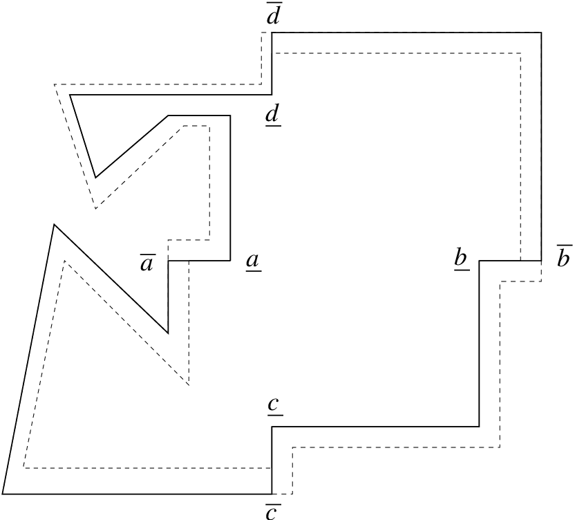

It should be clear that for a given approximation of constructed as described above there is a strictly positive such that the distance between and the portions of that belong to and is not smaller than , and the distance between the union , two counterclockwise segments of , and is also not smaller than . On the other hand, for any , there exists such that for all , is contained inside the -neighborhood of with the counterclockwise segment (resp., ) in the -neighborhood of the counterclockwise segment (resp., ). This implies that for large enough, any blue path crossing inside from the counterclockwise segment of to the counterclockwise segment of must have a subpath that stays inside and crosses between the counterclockwise segment of and the counterclockwise segment of . Therefore the crossing probability is a lower bound for for all , so that
| (23) |
as desired (the equality uses Smirnov’s result, Theorem 4, for fixed ).
We now note that as , . This allows us to use the continuity of Cardy’s formula (Lemma B.2 in Appendix Appendix B: Sequences of Conformal Maps) to obtain
| (24) |
From this and (23) it follows that
| (25) |
The remaining part of the proof involves defining a domain analogous to but with the property that the probability of an appropriate crossing, such that
| (26) |
is an upper bound for for all large enough. (The details of the construction of are analogous to those of ; we leave them to the reader.) This shows that
| (27) |
which, combined with (25), implies
| (28) |
and concludes the proof.
We note that Theorem 6, combined with the continuity of Cardy’s formula in the shape of the domain (for admissible domains) and positions of the four points on the boundary (Lemma B.2), implies the convergence of crossing probabilities to Cardy’s formula locally uniformly in the shape of the domain with respect to the uniform metric on curves, and in the location of the four points on the boundary with respect to the Euclidean metric; i.e., for an admissible domain with (with the notation used in Theorem 6), , and such that for all admissible domains with and , , where is Cardy’s formula and is the corresponding crossing probability.
Our next task is to show that the filling of any subsequential scaling limit of the percolation exploration process satisfies the spatial Markov property. Let us start with some notation. First of all, suppose that is a Jordan domain, and and are two points on . Define the discrete filling (or simply filling) at time of a percolation exploration path (with a given parametrization) inside (the -approximation of) from (the e-vertex closest to) to (the e-vertex closest to) to be the union of the hexagons explored up to time and those unexplored hexagons from which it is not possible to reach without crossing an explored hexagon or (in other words, this is the set of hexagons that at time have been explored or are disconnected from by the exploration path).
Consider a sequence of Jordan domains such that , where are two distinct points on . Denote by the percolation exploration path inside (the -approximation of) from (the e-vertex closest to) to (the e-vertex closest to) .
Notice that we can couple the paths simultaneously for all values of and by using the same percolation configuration to generate all of them. We can then apply the results of [2] to conclude that there exists a subsequence such that the law of converges to some limiting law for a process supported on (Hölder) continuous curves inside from to . The filling of , appearing in the next theorem, is defined just above Equation (17).
Theorem 7.
For any subsequential limit process of the percolation exploration path defined above, the filling of , as a process, satisfies the spatial Markov property.
Proof. Let be a subsequence such that the law of converges to some limiting law supported on continuous curves inside from to . We will prove the spatial Markov property by showing that as defined in the proof of Theorem 5 are jointly distributed like the corresponding hull variables, which do have the spatial Markov property. For each , let denote the filling at time of (with some parametrization – we do not need to worry about the choice of parametrization here). It follows from the Markovian character of the percolation exploration process that, for all , the filling of the percolation exploration path satisfies a suitably adapted (to the discrete setting) spatial Markov property. (In fact, the percolation exploration path satisfies a stronger property – roughly speaking, that the future of the path given the filling of the past is distributed as a percolation exploration path in the original domain from which the filling of the past has been removed.)
To be more precise, let be a conformal transformation that maps to such that and and let denote the first exit time of from defined as the first time an explored hexagon intersects the image under of the semi-circle . Define recursively as the first exit time of from , where is a conformal map from to that maps to and to . We also define , so that , and the (discrete-time) stochastic process for . The Markovian character of the percolation exploration process implies that, for every , is a Markov process (in ). In order to study the limit as of , we first need to analyze in more detail the mappings .
The conformal transformations are defined as follows, with an arbitrary multiplicative factor . We choose to be the composition of two maps, where , is the conformal transformation that maps onto with and (we are assuming for simplicity that the domain contains the origin; if that is not the case, one can think of a translated domain that does contain the origin), while is the inverse of the transformation
| (29) |
that maps onto , where is chosen so that and can be chosen so that , and , which means that maps to and to , so that indeed maps to and to .
Since converges in distribution to , we can find two coupled versions of and on some probability space such that converges to for all ; in the rest of the proof we work with these new versions which, with a slight abuse of notation, we denote with the same names as the original ones. Let be a conformal transformation that maps to such that and and let denote the first time hits , with . Define recursively as the first time hits , with , where is a conformal map from to that maps to and to . We also define , so that , and the (discrete-time) stochastic process . As above, we choose the conformal transformation to be the composition of two maps, where , is the conformal transformation that maps onto with and (once again, we are assuming for simplicity that the domain contains the origin; if that is not the case, one can think of a translated domain that does contain the origin), while is the inverse of the transformation
| (30) |
that maps onto , where is chosen so that and can be chosen so that , and , which means that maps to and to , so that indeed maps to and to .
Analogous quantities can be defined for the trace of chordal . For clarity, they will be indicated here by the superscript ; e.g., , , and . We want to show recursively that, for any , as , converge jointly in distribution to . By recursively applying Theorem 6 and Lemma A.1, we can then conclude that are jointly equidistributed with the corresponding hull variables (at the corresponding stopping times) . Since the latter do satisfy the spatial Markov property, so will the former, as desired.
The zeroth step consists in noticing that the convergence of to as allows us to apply Radó’s theorem (i.e., Theorem 9 of Appendix Appendix B: Sequences of Conformal Maps) to show that converges to uniformly in . This, together with the convergence of to and to , implies that converges to and to . Therefore, we also have the convergence of to and we can conclude that converges to uniformly on compact subsets of , which implies that the boundary of converges to the boundary of in the uniform metric on continuous curves.
Starting from there, the first step of our recursion argument is organized as follows:
- (1)
- (2)
, but also , by (1).
- (3)
, but also , by Corollary B.1.
- (4)
, but also , by (3).
At this point, we are in the same situation as at the zeroth step, but with , and replaced by , and respectively, and we can proceed by recursion. As explained above, the theorem then follows from the fact that the hull variables do posses the spatial Markov property.
In what follows we will show that the “number of arms” bounds [16] and Lemma A.2 below imply the convergence of to , and that the conditions to apply Theorem 6, Lemma A.2 and Corollary B.1 are always satisfied. (This last point boils down to showing that the domains and are admissible for all .) We begin by showing first that, as , converges in distribution to (which also implies that converges in distribution to ), from which it follows that converges in distribution to .
Consider and ; they are both composed of two domains (which “meet” at and respectively), which we denote by and and by and , respectively (see Figure 18).

It follows from [2] that for some further subsequence of the ’s (which we denote by simply replacing by ), converge jointly in distribution to some limit; we already know that must converge to and want to use this fact and a suitably adapted triangular array version of Lemma 5.2 (whose validity does not rely on statement (S)) to conclude that the limit is unique and coincides with . (Notice that and are two of the (many) domains in produced by the exploration process started at and stopped when it first hits the image under of the semi-circle , so we are in a context close to that of Lemma 5.2).
First of all, we need to show that the scaling limit of touches the image of the semi-circle under at a single point. This follows immediately from the definition of the stopping time for every fixed (with the map ), but it could fail to be true in the limit . The fact that it holds true in the limit is a direct consequence of Lemma A.2 below (in fact, a simpler version concerning Jordan domains would suffice here, but not when we iterate the argument – see below), which also implies that the single point at which the scaling limit of touches the image of the semi-circle under coincides with the limit of and with .
Therefore, if we remove the single point , the scaling limit of the boundary of splits into a left and a right part (corresponding to the scaling limit of the leftmost yellow and the rightmost blue -paths of hexagons explored by , respectively) that do not touch the image of the semi-circle under .
Moreover, Lemma A.3 below implies that if has a “close encounter” with , then it touches . Analogously, the standard bound on the probability of six crossings of an annulus [16], used repeatedly before, implies that wherever has a “close encounter” with itself, there is touching (see the proof of Lemma 5.1). These two observations assure that the scaling limit of is almost surely a filling (of ), i.e., a closed connected set whose complement in is simply connected. From the same bound on the probability of six crossings of an annulus, we can also conclude that the scaling limits of the left and right boundaries of are almost surely simple (continuous) curves, as in the proof of Lemma 5.1.
It is also possible to conclude that the intersection of the scaling limit of the left and right boundaries of with the boundary of almost surely does not contain arcs of positive length. In fact, if that were the case, it would be possible to find a subdomain with three counterclockwise points on its boundary such that the probability that an exploration path started at and stopped when it first hits the arc of has a positive probability, in the scaling limit, of hitting at or , contradicting Cardy’s formula (which, by Theorem 6, holds for all subsequential scaling limits). This means that the scaling limit of almost surely satisfies the condition in (17) and is therefore a hull. It says as well that, almost surely, the scaling limit of does not “stick” to the boundary of , which implies that also satisfies the condition in (17) and is therefore a hull.
It also implies that and are admissible domains since the part of the boundary of either or that belongs to the boundary of can be split up, by removing the single point , into two pieces which are, by an application of the proof of Lemma 5.1, simple continuous curves, while the remaining part of the boundary of either or is a Jordan arc whose interior does not touch the hull . (Notice however, that they need not be Jordan domains because has cut-points with positive probability – see Figure 19). This will be important later, when we need to apply Lemma A.1 (and therefore Theorem 6), Corollary B.1 and Lemmas A.2-A.3 again.
Then, since hulls are characterized by their “envelope” (see Lemma A.1 and the discussion preceding it), the joint convergence in distribution of to would be enough to conclude that converges to as , and in fact that converges in distribution to (and this will be valid also for the original subsequence and not just for the further subsequence ). In order to get that, as explained before, we can use the convergence in distribution of to and apply almost the same arguments as used in the proof of Lemma 5.2. The only difference is that, in proving claim (C), we cannot use the bound on the probability of three crossings of an annulus centered at a boundary point because we are not necessarily dealing with a convex domain. To replace that bound we use once again Lemmas A.2-A.3 below (a simpler version concerning Jordan domains would again suffice here, but not when we iterate the argument – see below).
We can then conclude that converges in distribution to , which in turn implies the joint convergence in distribution of to and concludes the first step of the argument.
We next need to prove that converges in distribution to . Since we have already proved the convergence of to , we claim that all we really need to prove is the convergence of to . To see this, notice that is distributed like the hull of a percolation exploration path inside . Besides, the convergence in distribution of to implies that we can find versions of and on some probability space such that converges to and converges to for all . These two observations imply that, if we work with the coupled versions of and , we are in the same situation as before, but with (resp., ) replaced by (resp., ) and (resp., ) by (resp., ). As already remarked, and are admissible domains, which allows us to use Theorem 6 (and therefore Lemma A.1), Corollary B.1 and Lemmas A.2-A.3.
Then the conclusion that converges in distribution to follows from the same arguments as before, again using Corollary B.1 and Lemmas A.2-A.3. In order to get claim (C), in places where the exploration path comes close to the boundary of the past hull we can use the bound on the probability of six crossings of an annulus in the plane (as already seen in the case of the proof of Theorem 1), while in places where it comes close to the remaining portion of the boundary (i.e., or the Jordan arc in Figure 19) we can use Lemmas A.2-A.3.

We can now iterate those same arguments times, for any . It is in fact easy to see by induction that the domains and that appear in the successive steps are admissible for all . Therefore we can keep using Theorem 6 (and therefore Lemma A.1), Corollary B.1 and Lemmas A.2-A.3. If we keep track at each step of the previous ones, in the spirit of Theorem 1, this provides the joint convergence of all the curves and fillings involved at each step and concludes the proof of Theorem 7.
Lemma A.2.
Let be a sequence of domains admissible with respect to and let be the percolation exploration path in started at and stopped when it first hits the counterclockwise arc of . Assume that, as , converges to , where is a domain admissible with respect to and . Let , where is the event that contains a segment that stays within and has a double crossing of the annulus without that segment touching , and is the event that enters , but is stopped outside and does not touch . Then, for any ,
| (31) |
Essentially, this means that as (and ), it becomes increasingly unlikely that the exploration path ever comes close to without quickly touching nearby.
Lemma A.2 easily implies the following result, used in Theorem 7 to show that if touches , then touches nearby, for large enough.
Lemma A.3.
With the notation and assumptions of Lemma A.2,
| (32) |
Proof. First of all notice that for in
but not in and not in , the events
and
are exactly the same because
the exploration path is, by definition, stopped on .
Therefore, we only have to prove that the event corresponding to the union over
of has probability
going to zero as .
We already know from Lemma A.2 that
happens with small
probability for those points.
This is, however, not sufficient because the exploration path could enter
, then exit , and then re-enter it
and touch inside , which is not an event in
.
But such an event would imply that first
touches inside one of the two balls of radius
centered at and , and by an application of Cardy’s formula
the probability that the latter happens goes to zero as
.
The proof of Lemma A.2 is partly based on relating the failure of (31) to the occurrence with strictly positive probability of certain continuum limit “mushroom” events (see Lemma A.5) that we will show must have zero probability because otherwise there would be a contradiction to Lemma A.4, which itself is a consequence of the continuity of Cardy’s formula with respect to the domain boundary. In both of the next two lemmas, we denote by any subsequence limit of the probability measures for the collection of all colored (blue and yellow) -paths on all of , in the Aizenman-Burchard sense (see Remark 2.1). We recall that in our notation, represents an open domain and , represent closed segments of its boundary. In Lemma A.4 below, we restrict attention to a Jordan domain since that case suffices for the use of Lemma A.4 in the proof of Lemma A.2.
Lemma A.4.
For , with a Jordan domain, consider the following crossing events, , where denotes either blue or yellow and :
Then .
Proof. The proof is similar to that of Theorem 6, but easier because is here a Jordan domain. Indeed, it is enough to construct a new Jordan domain (with appropriately selected points on the boundary and corresponding events ) such that the occurrence of in implies the occurrence of in and with as . The continuity of Cardy’s formula (Lemma B.2 in Appendix Appendix B: Sequences of Conformal Maps) does the rest.
Lemma A.5.
For as in Lemma A.2, , and , we define , the yellow “mushroom” event (at ), to be the event that there is a yellow path in from to and a blue path in , between some pair of distinct points in , that passes through and such that this blue path is between and the yellow path (see Figure 20). We similarly define with the colors interchanged and where denotes blue or yellow. Then for any deterministic domain and any , .

Proof. If for some , then there is some segment of of diameter not larger than such that
| (33) |
Choose any point and consider the new domain whose boundary consists of the correctly chosen (as we explain below) segment of the circle between the two points where first hits on either side of , together with the segment from to of (see Figure 21).

The correct circle segment between and is the (counter) clockwise one if is between and along when is oriented (counter) clockwise. It is also not hard to see that since , is a Jordan domain, so that Lemma A.4 can be applied. In the new domain , is the same curve segment as it was in the old domain , but is now a segment of the circle . It should be clear that
| (34) |
which yields a contradiction of Lemma A.4 if
.
Proof of Lemma A.2. We first note that since the probability in (31) is nonincreasing in , we may assume that , as requested by Lemma A.5.
Let us first consider the simpler case of in which . We follow the exploration process until time , when it first touches for some , and consider the annulus . Let be the leftmost yellow -path and the rightmost blue -path in at time that cross . and split the annulus into three sectors that, for simplicity, we will call the central sector, containing the crossing segment of the exploration path, the yellow (left) sector, with as part of its boundary, and the blue (right) sector, the remaining one, with as part of its boundary.
We then look for a yellow “lateral” crossing within the yellow sector from to and a blue lateral crossing within the blue sector from to . Notice that the yellow sector may contain “excursions” of the exploration path coming off , producing nested yellow and blue excursions off , and the same for the blue sector. But for topological reasons, those excursions are such that for every group of nested excursions, the outermost one is always yellow in the yellow sector and blue in the blue sector. Therefore, by standard percolation theory arguments, the conditional probability (conditioned on at time ) to find a yellow lateral crossing of the yellow sector from to is bounded below by the probability to find a yellow circuit in an annulus with inner radius and outer radius . An analogous statement holds for the conditional probability (conditioned on at time and also on the entire percolation configuration in the yellow sector) to find a blue lateral crossing of the blue sector from to . Thus for any fixed , by an application of the Russo-Seymour-Welsh lemma [27, 29], the conditional probability to find both a yellow lateral crossing within the yellow sector from to and a blue lateral crossing within the blue sector from to goes to one as .
But if such yellow and blue crossings are present, the exploration path is forced to touch before exiting , and if that happens, the exploration process is stopped, so that it will never exit and the union over of cannot occur. This concludes the proof of this case.
Let us now consider the remaining case in which . The basic idea of the proof is then that by straightforward weak convergence and related coupling arguments, the failure of (31) would imply that some subsequence limit would satisfy , which would contradict Lemma A.5. This is essentially because the close approach of an exploration path on the -lattice to without quickly touching nearby yields one two-sided colored -path (the “perimeter” of the portion of the hull of the exploration path seen from a boundary point of close approach) and a one-sided -path of the other color belonging to the percolation cluster not seen from the boundary point (i.e., shielded by the two-sided path). Both the two-sided path and the one-sided one are subsets of .
Assume by contradiction that (31) is false, so that close encounters without touching happen with bounded away from zero probability. Consider for concreteness an exploration path that has a close approach to a point in the counterclockwise arc . The exploration path may have multiple close approaches to with differing colors of the perimeter as seen from , but for topological reasons, the last time the exploration path comes close to , it must do so in such a way as to produce a yellow -path (seen from ) that crosses twice, and a blue path that crosses it once (see Figure 22). This is so because the exploration process that produced ended somewhere on (and outside ), which is to the right of (i.e., clockwise to) .

The presence of implies that there are a yellow leftmost -path and a yellow rightmost -path (looking at from inside ) crossing the annulus . The paths and split the annulus into three sectors, that we will call the central sector, containing , the left sector, with as part of its boundary, and the right sector, with as part of its boundary. Again for topological reasons, all other monochromatic crossings of the annulus are contained in the central sector, including at least one blue path . As in the previous case, the left and right sectors can contain nested monochromatic excursions off , but this time for every group of excursions, the outermost one is yellow in both sectors.
Now consider the annulus .
We look for a yellow lateral crossing within the left sector
from to and a yellow lateral crossing
within the right sector from to .
Since the outermost excursions in both sectors are yellow,
the conditional probability to find a yellow lateral crossing
within the left sector from to is bounded
below by the probability to find a yellow circuit in an annulus with
inner radius and outer radius ,
and an analogous statement holds for the conditional probability
to find a yellow lateral crossing within the right sector from
to .
Thus for any fixed , by an application of the
Russo-Seymour-Welsh lemma [27, 29], the conditional
probability to find both yellow lateral crossings goes to one
as .
But the presence of such yellow crossings would produce a (blue)
mushroom event, leading to a contradiction with Lemma A.5.
We are finally ready to prove the main result of this section which implies statement (S) at the beginning of Section 5.
Corollary A.1.
Consider a sequence of Jordan domains with two distinct selected points on their boundaries . Assume that , where is a Jordan domain with two distinct selected points on its boundary . Denote by the percolation exploration path inside (the -approximation of) from (the e-vertex closest to) to (the e-vertex closest to) . Then for any sequence , as , converges in distribution to the trace of chordal inside from to .
Proof. It follows from [2] that converges in distribution along subsequence limits . Since we have proved that the filling of any such subsequence limit satisfies the spatial Markov property (Theorem 7) and the exit distribution of is determined by Cardy’s formula (Theorem 6), we can deduce from Theorem 5 that the limit is unique and that the law of converges, as , to the law of the trace of chordal inside from to .
Appendix B: Sequences of Conformal Maps
In this appendix, we give some results about sequences of conformal maps that are used in various places throughout the paper. For more details, the interested reader should consult [24].
Definition B.1.
(see Section 1.4 of [24]) Let be given and let be domains with . We say that as with respect to in the sense of kernel convergence if
- 1.
either , or else is a domain with such that some neighborhood of every lies in for large ; and
- 2.
for there exist such that as .
It is clear from the definition that every subsequence limit also converges to and it is also easy to see that the limit is uniquely determined. With this definition we can now state Carathéodory’s kernel theorem [9].
Theorem 8.
(see Theorem 1.8 of [24]) Let map conformally onto with and . If , let ; otherwise let map conformally onto with and . Then, as , locally uniformly in if and only if with respect to .
The next result, Radó’s theorem [25], deals with sequences of Jordan domains and is used in the main body of the paper. In this case the conformal maps have a continuous extension to .
Theorem 9.
(see Theorem 2.11 of [24]) For , let and be Jordan curves parametrized respectively by and , , and let and be conformal maps from onto the inner domains of and such that and , for all . If as uniformly in then as uniformly in .
The type of convergence of sequences of Jordan domains to a Jordan domain encountered in the main body of the paper (i.e., in the sense that converges, as , to in the uniform metric (2) on continuous curves) is clearly sufficient to apply Theorem 9. In Appendix Appendix A: Convergence of the Percolation Exploration Path, however, we have to deal with domains that are not Jordan, and therefore we cannot use Radó’s theorem. The tools needed to deal with those situations are described below.
Definition B.2.
(see Section 2.2 of [24]) The closed set is called locally connected if for every there is such that, for any two points with , we can find a continuum with diameter smaller than and with .
In the definition above, a continuum denotes a compact connected set with more than one point. We remark that every continuous curve (with more than one point) is a locally connected continuum (the converse is also true: every locally connected continuum is a curve). The concept of local connectedness gives a topological answer to the problem of global extension of a conformal map to the domain boundary, as follows.
Theorem 10.
(see Continuity Theorem in Section 2.1 of [24]) Let map the unit disk conformally onto . Then the function has a continuous extension to if and only if is locally connected.
When has a continuous extension to , we do not distinguish between and its extension. This is always the case for the conformal maps considered in this paper. The problem wether this extension is injective on has also a topological answer, as follows.
Theorem 11.
When considering sequences of domains whose boundaries are locally connected the following definition is useful.
Definition B.3.
(see Section 2.2 of [24]) The closed sets are uniformly locally connected if, for every , there exists independent of such that any two points with can be joined by continua of diameter smaller than .
The convergence of domains used in this paper (i.e., if in the uniform metric (2) on continuous curves) clearly implies kernel convergence, which immediately allows us to use Theorem 8. However, we need uniform convergence in . This is guaranteed by Radó’s theorem in the case of Jordan domains; in the non-Jordan case, sufficient conditions to have uniform convergence are stated in the next theorem.
Theorem 12.
(see Corollary 2.4 of [24]) Let be a sequence of bounded domains such that, for some , for all and such that is uniformly locally connected. Let map conformally onto with . If as for each , then the convergence is uniform in .
In order to use Theorem 12 in Appendix Appendix A: Convergence of the Percolation Exploration Path we need the following lemma. The definitions of admissible domain and the related notion of convergence are given just before Theorem 6 in Appendix Appendix A: Convergence of the Percolation Exploration Path.
Lemma B.1.
Let be a sequence of domains admissible with respect to and assume that, as , , where is a domain admissible with respect to . Then the sequence of closed sets is uniformly locally connected.
Proof. In order to prove the lemma, we claim that it suffices to focus on pairs of points on the boundaries, i.e., to show that: for every , there exists independent of such that any two points with can be joined by a continuum of diameter contained in the complement of .
To verify our claim, let us assume for the moment, and consider two points (but not necessarily in ) with , where . If (at least) one of the two points, say , is at distance greater than from , then we can connect and using the closed ball of radius centered at , since . If both points are at distance smaller than from , we can connect each point to a closest point on by a straight segment of length smaller than . Those two points on can then be connected to each other by a continuum of diameter contained in , and the union of with the two straight segments gives a continuum of diameter connecting with and contained in .
We now prove . Since in the uniform metric (2) on continuous curves, for every there exists such that for all , . The admissibility of implies that we can split its boundary into three Jordan arcs, , , , such that does not touch the interior of either or . We can do the same with , letting , and . Let and , , be parametrizations of and respectively, with for and .
Let us assume, by contradiction, that is false. Then there are indices (actually , but we abuse notation a bit) and points with (as ) that cannot be joined by a continuum of diameter contained in . By compactness considerations, we may assume that and as , with . Suppose that and belong to the interior of the same Jordan arc for all large enough. Let , , and . It follows that and , and since is a Jordan arc, . For large enough, the function maps the closed segment of between and onto a continuum in containing and whose diameter tends to zero as , leading to a contradiction with our assumption.
Similar reasoning gives a contradiction if and both belong to or both belong to for all large enough, since the concatenation of with or of with is still a Jordan arc. The above reasoning applies except when is on both and . When , one can paste together small Jordan arcs on and to get a suitable continuum leading to a contradiction. The sole remaining case is when for all large enough, belongs to the interior of and belongs to the interior of .
(Notice that we are ignoring the “degenerate” case in which coincides with the “last” [from ] double-point on , and is a simple loop. In that case and could converge to and or could still belong to for arbitrarily large ’s. However, in that case one can find two distinct points on , and , such that is admissible with respect to , and points and on converging to and respectively, and define accordingly new Jordan arcs, and , so that and for large enough. We assume that this has been done if necessary, and for simplicity of notation drop the primes.)
In this case let denote the closed straight line segment in the plane between and . Imagine that is oriented from to and let be the first point of intersected by and be the previous intersection of with . Clearly, . For large enough, cannot belong to either, or otherwise in the limit , would touch the interior of and . We deduce that for all large enough, . Since and are continuous curves and therefore locally connected, and belong to a continuum contained in whose diameter goes to zero as , and the same for and (with and replaced by and ).
Since the interior of does not intersect any portion of , it is either contained in or in its complement . If , we have a contradiction since the union of with and is contained in and is a continuum containing and whose diameter goes to zero as .
If the interior of is contained in , let us
consider a conformal map from onto .
Since is locally connected, the conformal map
extends continuously to the boundary of the unit disc.
Let , , ,
and .
The points are in counterclockwise
order on , so that any curve in
from to the counterclockwise arc
must cross the curve from to whose image under
is .
This implies that any curve in going from to the
counterclockwise arc of must
cross the (interior of the) line segment .
Then, in the limit , any curve in from to
the counterclockwise arc must contain the limit
point .
On the other hand, except for its starting and ending point, any
such curve is completely contained in , which implies that either
or else that (in the limit ) the counterclockwise
arc is the single point at .
We have already dealt with the former case.
In the latter case, one can paste together small Jordan arcs
from to , from to , and from to ,
and take the union with and (defined above) to
get a suitable continuum in
containing and , leading to a contradiction.
This concludes the proof.
Theorem 12, together with Theorem 8 and Lemma B.1, implies the following result, which is used in Appendix Appendix A: Convergence of the Percolation Exploration Path.
Corollary B.1.
With the notation and assumptions of Lemma B.1 (and also assuming that and contain the origin), let map conformally onto with and , and map conformally onto with and . Then, as , uniformly in .
Proof. As already remarked, the convergence of
to in the uniform metric (2) on continuous curves
(which is part of the definition of )
easily implies that the conditions in Carathéodory’s kernel theorem
(Theorem 8) are satisfied and therefore that
converges to locally uniformly in , as .
By an application of Lemma B.1, the sequence
is uniformly locally connected, so that
we can apply Theorem 12 to conclude that, as ,
converges to uniformly in .
We conclude this appendix with a simple lemma, used in the proof of Theorem 6, about the continuity of Cardy’s formula with respect to the shape of the domain and the positions of the four points on the boundary.
Lemma B.2.
Proof. Let be the conformal map that takes onto with and , and let denote the conformal map from onto with and ; let , , , , , , , and . We can apply Corollary B.1 to conclude that, as , converges to uniformly in . This, in turn, implies that, as , , , , and .
Cardy’s formula for a crossing inside from the counterclockwise segment of to the counterclockwise segment of is given by
| (35) |
where
| (36) |
Because of the continuity of in , , , , and the continuity of Cardy’s formula (35) in , the convergence of , , and immediately implies the convergence of to .
Acknowledgements. We are grateful to Greg Lawler, Oded Schramm and Wendelin Werner for various interesting and useful conversations and to Stas Smirnov for communications about a paper in preparation. We note in particular that a discussion with Oded Schramm at the November 2004 Northeast Probability Seminar at the CUNY Graduate Center, about dependence of exploration paths with respect to small changes of domain boundaries, pointed us in a direction that eventually led to Lemmas A.2-A.5. F. C. thanks Wendelin Werner for an invitation to Université Paris-Sud 11, and Vincent Beffara and Luiz Renato Fontes for many helpful discussions. We are especially grateful to Vincent Beffara for pointing out a gap in a preliminary version of Appendix Appendix A: Convergence of the Percolation Exploration Path. We thank Lai-Sang Young for comments about the presentation of our results. F. C. acknowledges the kind hospitality of the Courant Institute where part of this work was completed.
References
- [1] M. Aizenman, Scaling limit for the incipient spanning clusters, in Mathematics of Multiscale Materials; the IMA Volumes in Mathematics and its Applications (K. Golden, G. Grimmett, R. James, G. Milton and P. Sen, eds.), Springer (1998).
- [2] M. Aizenman and A. Burchard, Hölder regularity and dimension bounds for random curves, Duke Math. J. 99, 419-453 (1999).
- [3] M. Aizenman, B. Duplantier and A. Aharony, Connectivity exponents and the external perimeter in independent percolation, Phys. Rev. Lett. 83, 1359-1362 (1999).
- [4] A. A. Belavin, A. M. Polyakov and A. B. Zamolodchikov, Infinite conformal symmetry of critical fluctuations in two dimensions, J. Stat. Phys. 34, 763-774 (1984).
- [5] A. A. Belavin, A. M. Polyakov and A. B. Zamolodchikov, Infinite conformal symmetry in two-dimensional quantum field theory, Nucl. Phys. B 241, 333-380 (1984).
- [6] P. Billingsley, Weak Convergence of Measures: Applications in Probability, Society for Industrial and Applied Mathematics, Philadelphia (1971).
- [7] F. Camia and C. M. Newman, Continuum Nonsimple Loops and 2D Critical Percolation, J. Stat. Phys. 116, 157-173 (2004).
- [8] F. Camia, C. M. Newman and V. Sidoravicius, Cardy’s formula for some dependent percolation models, Bull. Brazilian Math. Soc. 33, 147-156 (2002).
- [9] C. Carathéodory, Untersuchungen über die konformen Abbildungen von festen und veränderlichen Gebieten, Math. Ann. 72, 107-144 (1912).
- [10] J. L. Cardy, Critical percolation in finite geometries, J. Phys. A 25, L201-L206 (1992).
- [11] J. Cardy, Lectures on Conformal Invariance and Percolation, available at arXiv:math-ph/0103018 (2001).
- [12] R. Durrett, Probability: Theory and Examples, Third Edition, Duxbury Advanced Series (2004).
- [13] G. R. Grimmett, Percolation, second edition, Springer, Berlin (1999).
- [14] W. Kager and B. Nienhuis, A Guide to Stochastic Löwner Evolution and Its Applications, J. Phys. A 115, 1149-1229 (2004).
- [15] H. Kesten, Percolation Theory for Mathematicians, Birkhäuser, Boston (1982).
- [16] H. Kesten, V. Sidoravicius and Y. Zhang, Almost all words are seen in critical site percolation on the triangular lattice, Electr. J. Probab. 3, paper no. 10 (1998).
- [17] G. Lawler, Conformally Invariant Processes, in Lecture notes for the 2002 ICTP School and Conference on Probability, ICTP Lecture Notes Series, Vol. XVII (2004).
- [18] G. F. Lawler, Conformally Invariant Processes in the Plane, to be published by the American Mathematical Society (2005).
- [19] G. Lawler, O. Schramm and W. Werner, Values of Brownian intersection exponents I: Half-plane exponents, Acta Math. 187, 237-273 (2001).
- [20] G. Lawler, O. Schramm and W. Werner, One arm exponent for critical 2D percolation, Electronic J. Probab. 7, paper no. 2 (2002).
- [21] G. Lawler, O. Schramm and W. Werner, Conformal invariance of planar loop-erased random walk and uniform spanning trees, Ann. Prob. 32, 939-995 (2004).
- [22] G. Lawler, O. Schramm and W. Werner, Conformal restriction: the chordal case, J. Amer. Math. Soc. 16, 917-955 (2003).
- [23] A. M. Polyakov, Conformal symmetry of critical fluctuations, JETP Letters 12, 381-383 (1970).
- [24] Ch. Pommerenke, Boundary Behaviour of Conformal Maps, Springer-Verlag, Berlin (1992).
- [25] T. Radó, Sur la représentation conforme de domaines variables, Acta Sci. Math. (Szeged) 1, 180-186 (1923).
- [26] S. Rohde and O. Schramm, Basic properties of SLE, Ann. Math., to appear, preprint arXiv:math.PR0106036 (2003).
- [27] L. Russo, A note on percolation, Z. Wahrsch. Ver. Geb. 43, 39-48 (1978).
- [28] O. Schramm, Scaling limits of loop-erased random walks and uniform spanning trees, Israel J. Math. 118, 221-288 (2000).
- [29] P. D. Seymour, D. J. A. Welsh, Percolation probabilities on the square lattice, in Advances in Graph Theory (B. Bollobás ed.), Annals of Discrete Mathematics 3, North-Holland, Amsterdam, pp. 227-245 (1978).
- [30] S. Smirnov, Critical percolation in the plane: Conformal invariance, Cardy’s formula, scaling limits, C. R. Acad. Sci. Paris 333, 239-244 (2001).
- [31] S. Smirnov, Critical percolation in the plane. I. Conformal invariance and Cardy’s formula. II. Continuum scaling limit. (long version of [30], dated Nov. 15, 2001), available at http://www.math.kth.se/stas/papers/index.html.
- [32] S. Smirnov, in preparation.
- [33] S. Smirnov, private communication.
- [34] S. Smirnov and W. Werner, Critical exponents for two-dimensional percolation, Math. Rev. Lett. 8, 729-744 (2001).
- [35] W. Werner, Critical exponents, conformal invariance and planar Brownian motion, in Proceedings of the 3rd Europ. Congress of Math., Prog. Math., Vol. 202, 87-103 (2001).
- [36] W. Werner, SLEs as boundaries of clusters of Brownian loops, C. R. Math. Acad. Sci. Paris 337, 481–486 (2003).
- [37] W. Werner, Random planar curves and Schramm-Loewner Evolutions, in Lectures on probability theory and statistics, Lecture Notes in Math., Vol. 1840, Springer, Berlin, pp. 107-195 (2004).