跳到论文正文
W Papers独立论文阅读器 arXiv:math/0503715 论文正文 计算阅读时间 · 0%
引用这篇论文根据当前论文元数据生成,正式投稿前建议核对。


License: Assumed arXiv.org perpetual non-exclusive license
arXiv:math/0503715v1 [math.ST] 30 Mar 2005

On pointwise adaptive curve estimation with a degenerate random design

Stéphane Gaïffas Address: Laboratoire de Probabilités et Modèles Aléatoires, U.M.R. CNRS 7599 and Université Paris 7, 175 rue du Chevaleret, 75013 Paris Email address: gaiffas@math.jussieu.fr Laboratoire de Probabilités et Modèles Aléatoires
Université Paris 7, 175 rue du Chevaleret, 75013 Paris
email: gaiffas@math.jussieu.fr
Date: August 11, 2026
Abstract.

We consider the nonparametric regression with a random design model, and we are interested in the adaptive estimation of the regression at a point x0x_{0} where the design is degenerate. When the design density is β\beta-regularly varying at x0x_{0} and ff has a smoothness ss in the Hölder sense, we know from Gaïffas (2004) that the minimax rate is equal to n−s/(1+2s+β)ℓ(1/n)n^{-s/(1+2s+\beta)}\ell(1/n) where ℓ\ell is slowly varying. In this paper we provide an estimator which is adaptive both on the design and the regression function smoothness and we show that it converges with the rate (log⁡n/n)s/(1+2​s+β)​ℓ​(log⁡n/n)(\log n/n)^{s/(1+2s+\beta)}\ell(\log n/n). The procedure consists of a local polynomial estimator with a Lepski type data-driven bandwidth selector similar to the one in Goldenshluger and Nemirovski (1997) or Spokoiny (1998). Moreover, we prove that the payment of a log\log in this adaptive rate compared to the minimax rate is unavoidable.

Key words and phrases:
adaptive estimation, degenerate design, nonparametric regression, random design.
2000 Mathematics Subject Classification
62G05, 62G08

1. Introduction

1.1. The model

We observe nn pairs of random variables (Xi,Yi)∈ℝ×ℝ(X_{i},Y_{i})\in\mathbb{R}\times\mathbb{R} independent and identically distributed satisfying

(1.1) Yi=f⁡(Xi)+ξi,Y_{i}=f(X_{i})+\xi_{i},

where f:[0,1]→ℝf:[0,1]\rightarrow\mathbb{R} is the unknown signal to be recovered, the variables (ξi)(\xi_{i}) are centered Gaussian with variance σ2\sigma^{2} and independent of the design X1,…,XnX_{1},\ldots,X_{n}. The variables XiX_{i} are distributed with respect to a density μ\mu. We want to recover ff at a fixed point x0x_{0}.

The classical way to consider the nonparametric regression model is to take Xi=i/nX_{i}=i/n. In this model with an equispaced design the observations are homogeneously distributed over the unit interval. If we take the XiX_{i} random we can modelize cases with inhomogeneous observations as the design distribution is "far" from the uniform law. We allow here the density μ\mu to be degenerate (vanishing or exploding) and we are more precisely interested in the adaptive estimation of ff at a point where the design is degenerate, namely a point with very inhomogeneous data.

1.2. Motivations

The adaptive estimation of the regression function is a well-developed problem. Several adaptive procedures can be applied for the estimation of a function with unknown smoothness: nonlinear wavelet estimation (thresholding), model selection, kernel estimation with a variable bandwidth (the Lepski method), and so on.

Recent results dealing with the adaptive estimation of the regression function when the design is not equispaced or random include Antoniadis et al. (1997), Brown and Cai (1998), Wong and Zheng (2002), Maxim (2003), Delouille et al. (2004), Kerkyacharian and Picard (2004), among others. A natural question arises: what happens if we want to estimate adaptatively the regression function at a point where the design is degenerate? In Gaïffas (2004) we proved when μ\mu varies regularly at x0x_{0} that the minimax convergence rate ψn\psi_{n} over a Hölder type regularity class with smoothness s>0s>0 (around x0x_{0}) satisfies

ψn≍n−s/(1+2s+β)ℓ(1/n) as n→+∞,\psi_{n}\asymp n^{-s/(1+2s+\beta)}\ell(1/n)\text{ as }n\rightarrow+\infty,

where β\beta is the regular variation index of μ\mu at x0x_{0} (see definition 2) and ℓ\ell is slowly varying (the notation an≍bna_{n}\asymp b_{n} means 0<lim infan/bn⩽lim supan/bn<+∞0<\liminf a_{n}/b_{n}\leqslant\limsup a_{n}/b_{n}<+\infty). For the proof of the upper bound, a (non adaptive) linear procedure was used.

The next logical step is then to find a procedure able to recover ff with as less prior knowledge as possible on its smoothness and on the design density. On pointwise adaptive curve estimation (in the regression or the white noise model) see Lepski (1990), Lepski and Spokoiny (1997), Spokoiny (1998) and Brown and Cai (1998) for wavelet methods.

1.3. Organisation of the paper

We introduce the estimator in section 2. In section 3 we give upper bounds for this procedure conditionally on the design, see theorem 1 and in the regular variation framework, see theorem 2. In section 4 we prove that the obtained convergence rate is optimal, see theorem 3 and its corollary. We present numerical illustrations in section 5 for several datasets and we discuss in detail some points in section 6. Section 7 is devoted to the proofs and we recall some well-known facts on regularly varying functions in appendix.

2. The procedure

2.1. Local polynomial estimation

Let κ∈ℕ\kappa\in\mathbb{N} and h>0h>0 (the bandwidth). We define

Nn,h≜#{Xi such that Xi∈[x0−h,x0+h]},N_{n,h}\triangleq\#\{X_{i}\text{ such that }X_{i}\in[x_{0}-h,x_{0}+h]\},

and we introduce the pseudo-scalar product

⟨f,g⟩h≜1Nn,h​∑|Xi−x0|⩽hf⁡(Xi)​g​(Xi),\langle f\,,\,g\rangle_{h}\triangleq\frac{1}{N_{n,h}}\sum_{|X_{i}-x_{0}|\leqslant h}f(X_{i})g(X_{i}),

and ∥⋅∥h\|\cdot\|_{h} the corresponding pseudo-norm. Let ϕj​(x)=(x−x0)j\phi_{j}(x)=(x-x_{0})^{j} for j=0,…,κj=0,\ldots,\kappa. We introduce the matrix 𝐗h\mathbf{X}_{h} and the vector 𝐘h\mathbf{Y}_{h} with entries for 0⩽j,l⩽κ0\leqslant j,l\leqslant\kappa:

(2.1) (𝐗h)j,l=⟨ϕj,ϕl⟩h and (𝐘h)j=⟨Y,ϕj⟩h.(\mathbf{X}_{h})_{j,l}=\langle\phi_{j}\,,\,\phi_{l}\rangle_{h}\quad\text{ and }\quad(\mathbf{Y}_{h})_{j}=\langle Y\,,\,\phi_{j}\rangle_{h}.
Definition 1.

Let

f^h,κ={θ^h,0​ϕ0+θ^h,1​ϕ1+⋯+θ^h,κ​ϕκ when ​Nn,h>0, 0 when ​Nn,h=0,\widehat{f}_{h,\kappa}=\begin{cases}\,\widehat{\theta}_{h,0}\phi_{0}+\widehat{\theta}_{h,1}\phi_{1}+\cdots+\widehat{\theta}_{h,\kappa}\phi_{\kappa}&\text{ when }N_{n,h}>0,\\ \,0&\text{ when }N_{n,h}=0,\end{cases}

where θ^h\widehat{\theta}_{h} is the solution of the linear system

(2.2) 𝐗~h​θ=𝐘h,\widetilde{\mathbf{X}}_{h}\theta=\mathbf{Y}_{h},

where

𝐗~h≜𝐗h+Nn,h−1/2𝐈κ+1𝟏λ(𝐗h)⩽Nn,h−1/2,\widetilde{\mathbf{X}}_{h}\triangleq\mathbf{X}_{h}+N_{n,h}^{-1/2}\mathbf{I}_{\kappa+1}\mathbf{1}_{\lambda(\mathbf{X}_{h})\leqslant N_{n,h}^{-1/2}},

with λ⁡(M)\lambda(M) standing for the smallest eigenvalue of a matrix MM and 𝐈κ+1\mathbf{I}_{\kappa+1} the identity matrix in ℝκ+1\mathbb{R}^{\kappa+1}.

This procedure is slightly different from the classical version of the local polynomial estimator. We note that the correction term in 𝐗~h\widetilde{\mathbf{X}}_{h} entails λ(𝐗~h)⩾Nn,h−1/2\lambda(\widetilde{\mathbf{X}}_{h})\geqslant N_{n,h}^{-1/2}. On local polynomial estimation, see Stone (1980), Fan and Gijbels (1995, 1996), Spokoiny (1998) and Tsybakov (2003) among many others.

2.2. Adaptive bandwidth selection

The procedure selects the bandwidth hh in a set ℋ\mathcal{H} called the grid, which is a tuning parameter of the adaptive procedure. We can choose either an arithmetical or a geometrical grid

ℋ={ℋaarith=⋃i=1[(n−2)/a]{h2+[i​a]} for ​a⩾1, or ℋageom=⋃i=1[loga⁡n]{h[ai]} for ​a>1,\mathcal{H}=\begin{cases}\displaystyle\mathcal{H}_{a}^{\text{arith}}=\bigcup_{i=1}^{[(n-2)/a]}\{h_{2+[ia]}\}&\text{ for }a\geqslant 1,\text{ or }\\ \displaystyle\mathcal{H}_{a}^{\text{geom}}=\bigcup_{i=1}^{[\log_{a}{n}]}\{h_{[a^{i}]}\}&\text{ for }a>1,\end{cases}

where hi≜|X(i)−x0|h_{i}\triangleq|X_{(i)}-x_{0}| and where |X(i)−x0|⩽|X(i+1)−x0||X_{(i)}-x_{0}|\leqslant|X_{(i+1)}-x_{0}| for any i=1,…,n−1i=1,\ldots,n-1. Note that [x][x] stands for the integer part of xx. We define

ℋh≜{h′∈ℋ such that h′⩽h}.\mathcal{H}_{h}\triangleq\{h^{{}^{\prime}}\in\mathcal{H}\text{ such that }h^{{}^{\prime}}\leqslant h\}.

The bandwidth is selected as follows:

(2.3) H^n≜max{h∈ℋ|∀h′∈ℋh∀0⩽j⩽κ,|⟨f^h,κ−f^h′,κ,ϕj⟩h′|⩽σ∥ϕj∥h′Tn,h′,h},\widehat{H}_{n}\triangleq\max\Bigl\{h\in\mathcal{H}\big|\forall h^{{}^{\prime}}\in\mathcal{H}_{h}\,\forall 0\leqslant j\leqslant\kappa,\,|\langle\widehat{f}_{h,\kappa}-\widehat{f}_{h^{\prime},\kappa}\,,\,{\phi_{j}}\rangle_{h^{\prime}}|\leqslant\sigma\|\phi_{j}\|_{h^{\prime}}T_{n,h^{\prime},h}\Bigr\},

where f^h,κ\widehat{f}_{h,\kappa} is given by definition 1 and where the threshold Tn,h′,hT_{n,h^{\prime},h} is equal to

(2.4) Tn,h′,h≜{Cκ​Cp​Nn,h′−1​log⁡Nn,h+(Nn,h−a)−1​log⁡n if ​ℋ=ℋaarith,Cκ​Cp​Nn,h′−1​log⁡Nn,h+(1+a)​Nn,h−1​log⁡n if ​ℋ=ℋageom,T_{n,h^{\prime},h}\triangleq\begin{cases}\displaystyle C_{\kappa}\sqrt{C_{p}N_{n,h^{\prime}}^{-1}\log N_{n,h}}+\sqrt{(N_{n,h}-a)^{-1}\log n}&\text{ if }\mathcal{H}=\mathcal{H}_{a}^{\textup{arith}},\\ C_{\kappa}\sqrt{C_{p}N_{n,h^{\prime}}^{-1}\log N_{n,h}}+\sqrt{(1+a)N_{n,h}^{-1}\log n}&\text{ if }\mathcal{H}=\mathcal{H}_{a}^{\textup{geom}},\end{cases}

with Cκ≜1+κ+1C_{\kappa}\triangleq 1+\sqrt{\kappa+1}, Cp=8​(1+2​p)C_{p}=8(1+2p) where pp fits with the loss function in (3.1) and aa is the grid parameter. The estimator is then

(2.5) f^n​(x0)≜f^H^n,κ​(x0).\widehat{f}_{n}(x_{0})\triangleq\widehat{f}_{\widehat{H}_{n},\kappa}(x_{0}).

The selection rule (2.3) is similar to the method by Lepski, see Lepski (1990), Lepski et al. (1997) and Lepski and Spokoiny (1997) and is additionally to the original Lepski method sensitive to the design. This procedure is close to the one in Spokoiny (1998). See section 6.2 for more details on existing procedures in the literature.

3. Upper bounds

We measure a procedure f~n\widetilde{f}_{n} performance over a class Σ\Sigma (to be specified in the following) with the maximal risk

(3.1) (supf∈Σ𝔼f,μn​{|f~n​(x0)−f⁡(x0)|p})1/p,\bigl(\sup_{\displaystyle f\in\Sigma}\mathbb{E}_{\,f,\mu}^{\,n}\{|\widetilde{f}_{n}(x_{0})-f(x_{0})|^{p}\}\bigr)^{1/p},

where x0x_{0} is the estimation point and p⩾1p\geqslant 1. The expectation 𝔼f,μn\mathbb{E}_{\,f,\mu}^{\,n} in (3.1) is taken with respect to the joint law ℙf,μn\mathbb{P}_{f,\mu}^{n} of the observations (1.1).

3.1. Regular variation

The regular variation definition and main properties are due to Karamata (1930). On this topic we refer to Senata (1976), Geluk and de Haan (1987), Resnick (1987) and Bingham et al. (1989).

Definition 2 (Regular variation).

A continuous function ν:ℝ+→ℝ+\nu:\mathbb{R}^{+}\rightarrow\mathbb{R}^{+} is regularly varying at 00 if there is a real number β∈ℝ\beta\in\mathbb{R} such that

(3.2) ∀y>0,limh→0+ν⁡(y​h)/ν⁡(h)=yβ.\forall y>0,\quad\lim_{h\rightarrow 0^{+}}\nu(yh)/\nu(h)=y^{\beta}.

We denote by RV⁡(β)\mathrm{RV}(\beta) the set of all such functions. A function in RV⁡(0)\mathrm{RV}(0) is slowly varying.

Remark.

Roughly speaking, a regularly varying function behaves as a power function times a slower term. Typical examples of such functions are xβx^{\beta}, xβ​(log⁡(1/x))γx^{\beta}(\log(1/x))^{\gamma} and more generally any power function times a log\log or compositions of log\log to some power. For other examples, see in the references.

Definition 3.

If δ>0\delta>0 and ω∈RV⁡(s)\omega\in\mathrm{RV}(s) with s>0s>0 we define the class ℱδ​(x0,ω)\mathcal{F}_{\delta}(x_{0},\omega) of all functions f:ℝ→ℝf:\mathbb{R}\rightarrow\mathbb{R} such that

∀h⩽δ,infP∈𝒫ksup|x−x0|⩽h|f⁡(x)−P⁡(x−x0)|⩽ω⁡(h),\forall h\leqslant\delta,\quad\inf_{P\in\mathcal{P}_{k}}\sup_{|x-x_{0}|\leqslant h}|f(x)-P(x-x_{0})|\leqslant\omega(h),

where k=⌊s⌋k=\lfloor s\rfloor (the largest integer smaller than ss) and 𝒫k\mathcal{P}_{k} is the set of all the real polynomials with degree kk. We define ℓω​(h)≜ω⁡(h)​h−s\ell_{\omega}(h)\triangleq\omega(h)h^{-s} the slow variation term of ω\omega. If α>0\alpha>0 we define

𝒰⁡(α)≜{f:[0,1]→ℝ​ such that ​‖f‖∞⩽α}.\mathcal{U}(\alpha)\triangleq\bigl\{f:[0,1]\rightarrow\mathbb{R}\text{ such that }\|f\|_{\infty}\leqslant\alpha\bigr\}.

Finally, we define

Σδ,α​(x0,ω)≜ℱδ​(x0,ω)∩𝒰⁡(α).\Sigma_{\delta,\alpha}(x_{0},\omega)\triangleq\mathcal{F}_{\delta}(x_{0},\omega)\cap\mathcal{U}(\alpha).
Remark.

If ω⁡(h)=r​hs\omega(h)=rh^{s} for r>0r>0 we find back the classical Hölder regularity with radius rr. In this sense, the class ℱδ​(x0,ω)\mathcal{F}_{\delta}(x_{0},\omega) is a slight Hölder regularity generalisation.

3.2. Conditionally on the design

When nothing is known on the design density behaviour we can work conditionally on the design. Let 𝔛n\mathfrak{X}_{n} be the sigma-algebra generated by X1,…,XnX_{1},\ldots,X_{n}. We define

(3.3) Hn,ω≜min{h∈[0,1] such that ω(h)⩾σNn,h−1​log⁡n},H_{n,\omega}\triangleq\min\Bigl\{h\in[0,1]\text{ such that }\omega(h)\geqslant\sigma\sqrt{N_{n,h}^{-1}\log n}\Bigr\},

which is well defined for nn large enough (when ω⁡(1)⩾σ​log⁡n/n\omega(1)\geqslant\sigma\sqrt{\log n/n}). The quantity Hn,ωH_{n,\omega} makes the balance between the bias and the log\log-penalised variance of f^h,κ\widehat{f}_{h,\kappa} (see lemma 1) and therefore can be understood as the ideal adaptive bandwidth, see Lepski and Spokoiny (1997) and Spokoiny (1998). The log\log term in (3.3) is the payment for adaptation, see section 4.1. Let us define

Hn,ω∗≜max⁡{h∈ℋ|h⩽Hn,ω},H_{n,\omega}^{*}\triangleq\max\{h\in\mathcal{H}|h\leqslant H_{n,\omega}\},

and

(3.4) Rn,ω≜σ​Nn,Hn,ω∗−1​log⁡n.R_{n,\omega}\triangleq\sigma\sqrt{N_{n,H_{n,\omega}^{*}}^{-1}\log n}.

We define the diagonal matrix Λh≜diag​(‖ϕ0‖h−1,…,‖ϕκ‖h−1)\Lambda_{h}\triangleq\text{diag}(\|\phi_{0}\|_{h}^{-1},\ldots,\|\phi_{\kappa}\|_{h}^{-1}), the symmetrical matrix 𝒢h≜Λh​𝐗~h​Λh\mathcal{G}_{h}\triangleq\Lambda_{h}\widetilde{\mathbf{X}}_{h}\Lambda_{h} and λn,ω≜λ⁡(𝒢Hn,ω∗)\lambda_{n,\omega}\triangleq\lambda(\mathcal{G}_{H_{n,\omega}^{*}}). We define the event

(3.5) Ωh≜{X1,…,Xn are such that λ(𝐗h)>Nn,h−1/2 and Nn,h⩾2}.\Omega_{h}\triangleq\{X_{1},\ldots,X_{n}\text{ are such that }\lambda(\mathbf{X}_{h})>N_{n,h}^{-1/2}\text{ and }N_{n,h}\geqslant 2\}.

We note that Ωh∈𝔛n\Omega_{h}\in\mathfrak{X}_{n} and 𝐗h\mathbf{X}_{h} is invertible on Ωh\Omega_{h}. The next result shows that, conditional on 𝔛n\mathfrak{X}_{n}, f^n​(x0)=f^H^n,κ​(x0)\widehat{f}_{n}(x_{0})=\widehat{f}_{\widehat{H}_{n},\kappa}(x_{0}) converges with the rate Rn,ωR_{n,\omega} simultaneously over any Σ⁡(x0,ω)\Sigma(x_{0},\omega) when ω∈RV⁡(s)\omega\in\mathrm{RV}(s) with 0<s⩽κ+10<s\leqslant\kappa+1.

Theorem 1.

If ω∈RV⁡(s)\omega\in\mathrm{RV}(s), 0<s⩽κ+10<s\leqslant\kappa+1 and α>0\alpha>0 we have for any n⩾κ+1n\geqslant\kappa+1 on ΩHn,ω∗\Omega_{H_{n,\omega}^{*}}:

supf∈ΣHn,ω∗,α​(x0,ω)𝔼f,μn{Rn,ω−p|f^n(x0)−f(x0)|p|𝔛n}⩽c1λn,ω−p+c2(α∨1)p(logn)−p/2,\sup_{\displaystyle f\in\Sigma_{H_{n,\omega}^{*},\alpha}(x_{0},\omega)}\mathbb{E}_{\,f,\mu}^{\,n}\bigl\{R_{n,\omega}^{-p}|\widehat{f}_{n}(x_{0})-f(x_{0})|^{p}|\mathfrak{X}_{n}\bigr\}\leqslant c_{1}\lambda_{n,\omega}^{-p}+c_{2}(\alpha\vee 1)^{p}(\log n)^{-p/2},

where c1=c1​(p,κ,a)c_{1}=c_{1}(p,\kappa,a) and c2=c2​(p,κ,a,σ)c_{2}=c_{2}(p,\kappa,a,\sigma).

We will see that the probability of the event ΩHn,ω∗\Omega_{H_{n,\omega}^{*}} is large and that λn,ω\lambda_{n,\omega} is positive with a large probability when the design density is regularly varying (see lemma 9). Note that the upper bound in theorem 1 is non asymptotic in the sense that it holds for any n⩾κ+1n\geqslant\kappa+1. The random normalisation Rn,ωR_{n,\omega} is similar to the one in Guerre (1999), see section 6.2 for more details.

3.3. Regularly varying design

Definition 4.

For β>−1\beta>-1 and a neighbourhood WW of x0x_{0} we define

ℛ(x0,β)≜{μ density such that ∃ν∈RV(β)∀x∈W,μ(x)=ν(|x−x0|)}.\mathcal{R}(x_{0},\beta)\triangleq\bigl\{\mu\text{ density such that }\exists\nu\in\mathrm{RV}(\beta)\,\forall x\in W,\quad\mu(x)=\nu(|x-x_{0}|)\bigr\}.

We assume in all the following that μ∈ℛ⁡(x0,β)\mu\in\mathcal{R}(x_{0},\beta) for β>−1\beta>-1. Let hn,ωh_{n,\omega} be the smallest solution to

(3.6) ω⁡(h)=σ​log⁡n2​n​∫0hν⁡(t)​𝑑t,\omega(h)=\sigma\sqrt{\frac{\log n}{2n\int_{0}^{h}\nu(t)dt}},

and

(3.7) rn,ω≜ω⁡(hn,ω).r_{n,\omega}\triangleq\omega(h_{n,\omega}).

Equation (3.6) can be viewed as the deterministic counterpart to the equilibrium in (3.3). We define Cα,β≜(1+(−1)α)​β+1α+β+1C_{\alpha,\beta}\triangleq(1+(-1)^{\alpha})\frac{\beta+1}{\alpha+\beta+1} and the matrix 𝒢\mathcal{G} with entries (𝒢)j,l≜Cj+l,βC2​j,β​C2​l,β(\mathcal{G})_{j,l}\triangleq\frac{C_{j+l,\beta}}{\sqrt{C_{2j,\beta}C_{2l,\beta}}} for 0⩽j,l⩽κ0\leqslant j,l\leqslant\kappa and λκ,β≜λ⁡(𝒢)\lambda_{\kappa,\beta}\triangleq\lambda(\mathcal{G}). It is easy to see that λκ,β>0\lambda_{\kappa,\beta}>0.

Theorem 2.

If

  • •

    κ∈ℕ\kappa\in\mathbb{N}, β>−1\beta>-1, α>0\alpha>0 and ϱ>1\varrho>1,

  • •

    ω∈RV⁡(s)\omega\in\mathrm{RV}(s) for 0<s⩽κ+10<s\leqslant\kappa+1,

then the estimator f^n​(x0)=f^κ,H^n​(x0)\widehat{f}_{n}(x_{0})=\widehat{f}_{\kappa,\widehat{H}_{n}}(x_{0}) with the grid ℋ=ℋ1arith\mathcal{H}=\mathcal{H}_{1}^{\textup{arith}} satisfies

(3.8) ∀μ∈ℛ⁡(x0,β)lim supnsupf∈Σϱ​hn,ω,α​(x0,ω)𝔼f,μn​{rn,ω−p​|f^n​(x0)−f⁡(x0)|p}⩽C​λκ,β−p,\forall\mu\in\mathcal{R}(x_{0},\beta)\quad\limsup_{n}\sup_{\displaystyle f\in\Sigma_{\varrho h_{n,\omega},\alpha}(x_{0},\omega)}\mathbb{E}_{\,f,\mu}^{\,n}\bigl\{r_{n,\omega}^{-p}|\widehat{f}_{n}(x_{0})-f(x_{0})|^{p}\bigr\}\leqslant C\lambda_{\kappa,\beta}^{-p},

where C=C⁡(p,κ)C=C(p,\kappa). Moreover, we have

(3.9) rn,ω∼σ2​s/(1+2​s+β)​(log⁡n/n)s/(1+2​s+β)​ℓω,ν​(log⁡n/n)​ as ​n→+∞,r_{n,\omega}\sim\sigma^{2s/(1+2s+\beta)}(\log n/n)^{s/(1+2s+\beta)}\ell_{\omega,\nu}(\log n/n)\text{ as }n\rightarrow+\infty,

where ℓω,ν\ell_{\omega,\nu} is slowly varying.

Remark.

When ω⁡(h)=r​hs\omega(h)=rh^{s} (Hölder regularity) we have more precisely

rn,ω∼σ2​s/(1+2​s+β)​r(1+β)/(1+2​s+β)​(log⁡n/n)s/(1+2​s+β)​ℓs,ν​(log⁡n/n)​ as ​n→+∞.r_{n,\omega}\sim\sigma^{2s/(1+2s+\beta)}r^{(1+\beta)/(1+2s+\beta)}(\log n/n)^{s/(1+2s+\beta)}\ell_{s,\nu}(\log n/n)\text{ as }n\rightarrow+\infty.

Note that ℓ1​(h)=ℓω,ν​(h​log⁡(1/h))\ell_{1}(h)=\ell_{\omega,\nu}(h\log(1/h)) is also slowly varying, thus ℓ1​(1/n)=ℓω,ν​(log⁡n/n)\ell_{1}(1/n)=\ell_{\omega,\nu}(\log n/n) is a slow term.

3.4. Convergence rates examples

Let β>−1\beta>-1, r,sr,s be positive and α,γ\alpha,\gamma be any real numbers. If we take ν\nu such that ∫0hν⁡(t)​𝑑t=hβ+1​(log⁡(1/h))α\int_{0}^{h}\nu(t)dt=h^{\beta+1}(\log(1/h))^{\alpha} and ω⁡(h)=r​hs​(log⁡(1/h))γ\omega(h)=rh^{s}(\log(1/h))^{\gamma} then we find that (see section 7.3 for the computation details)

(3.10) rn,ω∼σ2​s/(1+2​s+β)r(β+1)/(1+2​s+β)(n(logn)α−1−γ⁡(1+β)/s)−s/(1+2s+β),r_{n,\omega}\sim\sigma^{2s/(1+2s+\beta)}r^{(\beta+1)/(1+2s+\beta)}\bigl(n(\log n)^{\alpha-1-\gamma(1+\beta)/s}\bigr)^{-s/(1+2s+\beta)},

where an∼bna_{n}\sim b_{n} mean limn→+∞an/bn=1\lim_{n\rightarrow+\infty}a_{n}/b_{n}=1. This rate has to be compared with the minimax rate from Gaïffas (2004):

σ2​s/(1+2​s+β)r(β+1)/(1+2​s+β)(n(logn)α−γ⁡(1+β)/s)−s/(1+2s+β),\sigma^{2s/(1+2s+\beta)}r^{(\beta+1)/(1+2s+\beta)}\bigl(n(\log n)^{\alpha-\gamma(1+\beta)/s}\bigr)^{-s/(1+2s+\beta)},

where the only difference is the α\alpha instead of α−1\alpha-1 in the log\log exponent. This loss is the payment for adaptation and is unavoidable in view of theorem 3 and its corollary. See section 4 for more details.

In the classical case, namely when the design is non-degenerate and ff is Hölder (ω⁡(h)=r​hs\omega(h)=rh^{s} and α=β=γ=0\alpha=\beta=\gamma=0) we find the usual pointwise minimax adaptive rate (see Lepski (1990), Brown and Low (1996)):

σ2​s/(1+2​s)​r1/(1+2​s)​(log⁡n/n)s/(1+2​s).\sigma^{2s/(1+2s)}r^{1/(1+2s)}(\log n/n)^{s/(1+2s)}.

When the design is again non-degenerate and the continuity modulus is equal to ω⁡(h)=r​hs​(log⁡(1/h))−s\omega(h)=rh^{s}(\log(1/h))^{-s} we find a convergence rate equal to

σ2​s/(1+2​s)r1/(1+2​s)n−s/(1+2s),\sigma^{2s/(1+2s)}r^{1/(1+2s)}n^{-s/(1+2s)},

which is the usual minimax rate, without the log\log term for payment for adaptation. Actually, this is a "toy" example since we have asked for more regularity than in the Hölder regularity. Note that in the degenerate design case, when α\alpha and γ\gamma are such that α=1+γ⁡(1+β)/s\alpha=1+\gamma(1+\beta)/s there is again no extra log\log factor.

4. Optimality

4.1. Payment for adaptation

The convergence rate of a linear estimator with an adaptive bandwidth choice can be well explained with a balance equation between its bias and variance terms. In our context this equation is

ω⁡(h)=σNn,h,\omega(h)=\frac{\sigma}{\sqrt{N_{n,h}}},

(see lemma 1) and a deterministic counterpart of this equilibrium is

(4.1) ω⁡(h)=σ2​n​∫0hν⁡(t)​𝑑t,\omega(h)=\frac{\sigma}{\sqrt{2n\int_{0}^{h}\nu(t)dt}},

see lemma 5. We proved in Gaïffas (2004) that the minimax rate ψn,ω\psi_{n,\omega} over Σδ,α​(x0,ω)\Sigma_{\delta,\alpha}(x_{0},\omega) is given by

(4.2) ψn,ω=ω⁡(γn,ω),\psi_{n,\omega}=\omega(\gamma_{n,\omega}),

where γn,ω\gamma_{n,\omega} is the smallest solution to (4.1). In a model with homogeneous information (the white noise or the regression model with an equidistant design) we know that such a balance equation cannot be realized: an adaptive estimator to the unknown smoothness without loss of efficiency is not possible for pointwise estimation, even if we know that the function belongs to one of two Hölder classes, see Lepski (1990), Brown and Low (1996) and Lepski and Spokoiny (1997) . This means that local adaptation cannot be achieved for free: we have to pay an extra log\log factor in the convergence rate, at least of order (log⁡n)2​s/(1+2​s)(\log n)^{2s/(1+2s)} when estimating a Hölder function with smoothness ss. The authors call this phenomenon payment for adaptation. We intend here to generalise this result to the regression with a degenerate random design.

4.2. Superefficiency

Let ss, r′<rr^{\prime}<r, be positive and δ⩽1\delta\leqslant 1, p>1p>1. We take ω⁡(h)=r​hs\omega(h)=rh^{s}, ω′​(h)=r′​hs\omega^{\prime}(h)=r^{\prime}h^{s} and the minimax rate ψn,ω\psi_{n,\omega} defined by (4.2). In view of lemma 6 we have

(4.3) ψn,ω∼cs,β,σ,rn−s/(1+2s+β)ℓs,ν(1/n) as n→+∞.\psi_{n,\omega}\sim c_{s,\beta,\sigma,r}n^{-s/(1+2s+\beta)}\ell_{s,\nu}(1/n)\text{ as }n\rightarrow+\infty.

We recall that in view of theorem 2 the "adaptive" rate rn,ωr_{n,\omega} defined by (3.7) is attained by the adaptive procedure f^n​(x0)\widehat{f}_{n}(x_{0}) simultaneously over several classes Σδ,α​(x0,ω)\Sigma_{\delta,\alpha}(x_{0},\omega) with ω∈RV⁡(s)\omega\in\mathrm{RV}(s) for any regularity s∈(0,κ+1]s\in(0,\kappa+1] and that

(4.4) rn,ω∼cs,β,σ,r​(log⁡n/n)s/(1+2​s+β)​ℓs,ν​(log⁡n/n)​ as ​n→+∞.r_{n,\omega}\sim c_{s,\beta,\sigma,r}(\log n/n)^{s/(1+2s+\beta)}\ell_{s,\nu}(\log n/n)\text{ as }n\rightarrow+\infty.
Theorem 3.

If an estimator f^n\widehat{f}_{n} based on (1.1) is asymptotically minimax over ℱδ​(x0,ω)\mathcal{F}_{\delta}(x_{0},\omega), that is

lim supnsupf∈ℱδ​(x0,ω)ψn,ω−p​𝔼f,μn​{|f^n​(x0)−f⁡(x0)|p}<+∞,\limsup_{n}\sup_{\displaystyle f\in\mathcal{F}_{\delta}(x_{0},\omega)}\psi_{n,\omega}^{-p}\,\,\mathbb{E}_{\,f,\mu}^{\,n}\{|\widehat{f}_{n}(x_{0})-f(x_{0})|^{p}\}<+\infty,

and if this estimator is superefficient at a function f0∈ℱδ​(x0,ω′)f_{0}\in\mathcal{F}_{\delta}(x_{0},\omega^{\prime}) in the sense that there is γ>0\gamma>0 such that

(4.5) lim supnψn,ω−p​nγ​p​𝔼f0,μn​{|f^n​(x0)−f0​(x0)|p}<+∞,\limsup_{n}\psi_{n,\omega}^{-p}\,n^{\gamma p}\,\,\mathbb{E}_{f_{0},\mu}^{n}\{|\widehat{f}_{n}(x_{0})-f_{0}(x_{0})|^{p}\}<+\infty,

then we can find a function f1∈ℱδ​(x0,ω)f_{1}\in\mathcal{F}_{\delta}(x_{0},\omega) such that

lim infnrn,ω−p​𝔼f1,μn​{|f^n​(x0)−f1​(x0)|p}>0.\liminf_{n}r_{n,\omega}^{-p}\,\,\mathbb{E}_{f_{1},\mu}^{n}\{|\widehat{f}_{n}(x_{0})-f_{1}(x_{0})|^{p}\}>0.

This theorem is a generalisation of a result by Brown and Low (1996) for the degenerate random design case. Of course, when the design is non-degenerate (0<μ⁡(x0)<+∞0<\mu(x_{0})<+\infty) the theorem remains valid and the result is barely the same as in Brown and Low (1996) with the same rates.

The theorem 3 is a lower bound for a superefficient estimator. Actually, the most interesting result for our problem is the next corollary.

4.3. An adaptive lower bound

Let 0<r2<r1<+∞0<r_{2}<r_{1}<+\infty and 0<s1<s2<+∞0<s_{1}<s_{2}<+\infty be such that ⌊s1⌋=⌊s2⌋=k\lfloor s_{1}\rfloor=\lfloor s_{2}\rfloor=k. If ωi​(h)=ri​hsi\omega_{i}(h)=r_{i}h^{s_{i}} we denote ℱi≜ℱδ​(x0,ωi)\mathcal{F}_{i}\triangleq\mathcal{F}_{\delta}(x_{0},\omega_{i}). Let ψn,i\psi_{n,i} be the minimax rate defined by (4.2) over ℱi\mathcal{F}_{i} for i=1,2i=1,2 and rn,1r_{n,1} be defined by (3.7) with ω=ω1\omega=\omega_{1} (the "adaptive" rate when the class is ℱ1\mathcal{F}_{1}). Note that ψn,i\psi_{n,i} satisfies (4.3) with s=sis=s_{i} and rn,1r_{n,1} satisfies (4.4) with s=s1s=s_{1}.

Corollary 1.

If an estimator f^n\widehat{f}_{n} is asymptotically minimax over ℱ1\mathcal{F}_{1} and ℱ2\mathcal{F}_{2}, that is for i=1,2i=1,2:

(4.6) lim supnsupf∈ℱiψn,i−p​𝔼f,μn​{|f^n​(x0)−f⁡(x0)|p}<+∞,\limsup_{n}\sup_{\displaystyle f\in\mathcal{F}_{i}}\psi_{n,i}^{-p}\,\,\mathbb{E}_{\,f,\mu}^{\,n}\{|\widehat{f}_{n}(x_{0})-f(x_{0})|^{p}\}<+\infty,

then this estimator also satisfies

(4.7) lim infnsupf∈ℱ1rn,1−p​𝔼f,μn​{|f^n​(x0)−f⁡(x0)|p}>0.\liminf_{n}\sup_{\displaystyle f\in\mathcal{F}_{1}}r_{n,1}^{-p}\,\,\mathbb{E}_{\,f,\mu}^{\,n}\big\{|\widehat{f}_{n}(x_{0})-f(x_{0})|^{p}\big\}>0.

Note that (4.7) contradicts (4.6) for i=1i=1 since limnψn,1/rn,1=0\lim_{n}\psi_{n,1}/r_{n,1}=0, thus there is no pointwise minimax adaptive estimator over two such classes ℱ1\mathcal{F}_{1} and ℱ2\mathcal{F}_{2} and the best achievable rate is rn,ir_{n,i}. The corollary 1 is an immediate consequence of theorem 3. Clearly, ℱ2⊂ℱ1\mathcal{F}_{2}\subset\mathcal{F}_{1} thus equation (4.6) entails that f^n\widehat{f}_{n} is superefficient at any function f0∈ℱ2f_{0}\in\mathcal{F}_{2}. More precisely, f^n\widehat{f}_{n} satisfies (4.5) with γ=(s2−s1)​(β+1)2​(1+2​s1+β)​(1+2​s2+β)>0\gamma=\frac{(s_{2}-s_{1})(\beta+1)}{2(1+2s_{1}+\beta)(1+2s_{2}+\beta)}>0 since n−γ​ℓ​(1/n)→0n^{-\gamma}\ell(1/n)\rightarrow 0 where ℓ≜ℓs1,ν/ℓs2,ν\ell\triangleq\ell_{s_{1},\nu}/\ell_{s_{2},\nu} and ℓ∈RV⁡(0)\ell\in\mathrm{RV}(0).

5. Simulations

5.1. Implementation of the procedure

For the estimation at a point xx, the procedure (2.3) selects the best symmetrical interval I=[x−h,x+h]I=[x-h,x+h] among several hh in the grid ℋ\mathcal{H}. We have implemented this procedure with non symmetrical intervals, which is a procedure similar to the one in Spokoiny (1998). First, we define similarly to section 2.1 for any I⊂[0,1]I\subset[0,1] the scalar product

⟨f,g⟩I≜∑Xi∈If⁡(Xi)​g​(Xi),\langle f\,,\,g\rangle_{I}\triangleq\sum_{X_{i}\in I}f(X_{i})g(X_{i}),

(it is convenient in this part to remove the normalisation term Nn,hN_{n,h} from the definition of the scalar product) and similarly to (2.1) we define the matrix 𝐗I\mathbf{X}_{I} with entries (𝐗I)j,l=⟨ϕj,ϕl⟩I(\mathbf{X}_{I})_{j,l}={\langle\phi_{j}\,,\,\phi_{l}\rangle}_{I} for 0⩽j,l⩽κ0\leqslant j,l\leqslant\kappa. We define in the same way 𝐘I\mathbf{Y}_{I}, and θ^I\widehat{\theta}_{I} is defined as the solution to

𝐗I​θ=𝐘I.\mathbf{X}_{I}\theta=\mathbf{Y}_{I}.

Note that if J⊂[0,1]J\subset[0,1], the vector 𝐅I,J\mathbf{F}_{I,J} with coordinates

(𝐅I,J)j=⟨f^I,κ−f^J,κ,ϕj⟩J/‖ϕj‖J(\mathbf{F}_{I,J})_{j}={\langle\widehat{f}_{I,\kappa}-\widehat{f}_{J,\kappa}\,,\,\phi_{j}\rangle}_{J}/\|\phi_{j}\|_{J}

(for 0⩽j⩽κ0\leqslant j\leqslant\kappa) satisfies

𝐅I,J=𝐇J​(θ^I−θ^J),\mathbf{F}_{I,J}=\mathbf{H}_{J}(\widehat{\theta}_{I}-\widehat{\theta}_{J}),

where 𝐇J\mathbf{H}_{J} is defined as the matrix with entries for 0⩽j,l⩽κ0\leqslant j,l\leqslant\kappa

(𝐇J)j,l≜∑Xi∈J(Xi−x)j+l∑Xi∈J(Xi−x)2​j.(\mathbf{H}_{J})_{j,l}\triangleq\frac{\sum_{X_{i}\in J}(X_{i}-x)^{j+l}}{\sqrt{\sum_{X_{i}\in J}(X_{i}-x)^{2j}}}.

The main steps of the procedure for the estimation at a point xx are then:

  1. (1)

    choose parameters a>1a>1, κ∈ℕ\kappa\in\mathbb{N} and m⩾κ+1m\geqslant\kappa+1,

  2. (2)

    sort the (Xi,Yi)(X_{i},Y_{i}) in (X(i),Y(i))(X_{(i)},Y_{(i)}) such that X(i)⩽X(i+1)X_{(i)}\leqslant X_{(i+1)},

  3. (3)

    find jj such that x∈[X(j),X(j+1)]x\in[X_{(j)},X_{(j+1)}] and #⁡{Xi|Xi∈[X(j),X(j+1)]}=m\#\{X_{i}|X_{i}\in[X_{(j)},X_{(j+1)}]\}=m,

  4. (4)

    build

    𝒢−=⋃i=0[loga⁡(j+1)]{X(j+1−[ai])},𝒢+=⋃i=0[loga⁡(n−j)]{X(j+[ai])},\mathcal{G}^{-}=\bigcup_{i=0}^{[\log_{a}(j+1)]}\{X_{(j+1-[a^{i}])}\},\hskip 28.45274pt\mathcal{G}^{+}=\bigcup_{i=0}^{[\log_{a}(n-j)]}\{X_{(j+[a^{i}])}\},
  5. (5)

    compute θ^I\widehat{\theta}_{I} and 𝐇I\mathbf{H}_{I} for all I∈𝒢≜𝒢−×𝒢+I\in\mathcal{G}\triangleq\mathcal{G}^{-}\times\mathcal{G}^{+},

  6. (6)

    if Nn,I≜#⁡{Xi|Xi∈I}N_{n,I}\triangleq\#\{X_{i}|X_{i}\in I\}, find

    I^≜argmaxI∈𝒢{Nn,I such that ∀J⊂I,J∈𝒢,∥𝐇J(θ^I−θ^J)∥∞⩽TI,J},\widehat{I}\triangleq\argmax_{I\in\mathcal{G}}\big\{N_{n,I}\text{ such that }\forall J\subset I,J\in\mathcal{G},\;\|\mathbf{H}_{J}(\widehat{\theta}_{I}-\widehat{\theta}_{J})\|_{\infty}\leqslant T_{I,J}\big\},

    where ∥⋅∥∞\|\cdot\|_{\infty} stands for the sup norm in ℝκ+1\mathbb{R}^{\kappa+1} and

    TI,J=σ^​(1+κ+1)​log⁡Nn,I+(1+a)​(Nn,J/Nn,I)​log⁡n,T_{I,J}=\widehat{\sigma}(1+\sqrt{\kappa+1})\sqrt{\log N_{n,I}}+\sqrt{(1+a)}\sqrt{(N_{n,J}/N_{n,I})\log n},

    with σ^\widehat{\sigma} for instance given by (6.3).

  7. (7)

    return the first coordinate of θ^I^\widehat{\theta}_{\widehat{I}}.

This procedure uses a geometrical grid, thus it is computationally feasible for reasonable choices of aa (a=1.05a=1.05 is used in the next section). The main steps of the procedure with an arithmetical grid are the same with a modification of the threshold, see (2.4). The procedure is implemented in C++ and is quite fast: it takes few seconds to recover the whole function at 300300 points on a modern computer.

5.2. Numerical illustrations

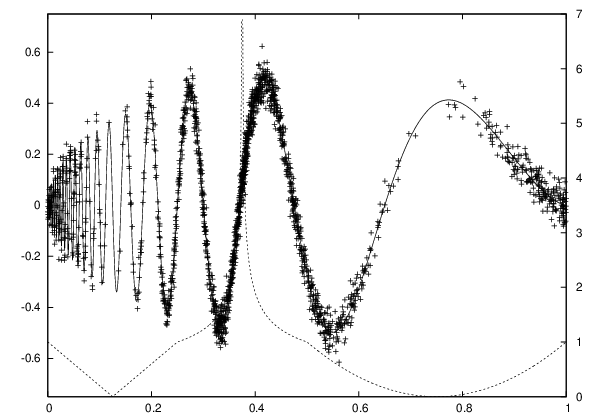
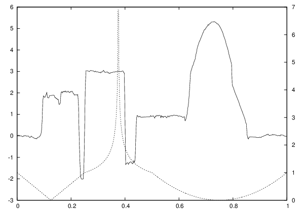
We use for our simulations the target functions from Donoho and Johnstone (1994). These functions are commonly used as benchmarks for adaptive estimators. We show in figure 1 the target functions and datasets with a uniform random design. The noise is Gaussian with σ\sigma chosen to have (root) signal-to-noise ratio 77. The sample size is n=2000n=2000. We show the estimates in figure 2. For all estimates we take κ=2\kappa=2, a=1.05a=1.05 and m=25m=25. We estimate at each point x=j/300x=j/300 with j=0,…,300j=0,\ldots,300.

Refer to caption
Refer to caption
Refer to caption
Refer to caption
Figure 1. Blocks, bumps, heavysine and doppler with Gaussian noise and uniform design.
Refer to caption
Refer to caption
Refer to caption
Refer to caption
Figure 2. Estimates based on the datasets in figure 1.

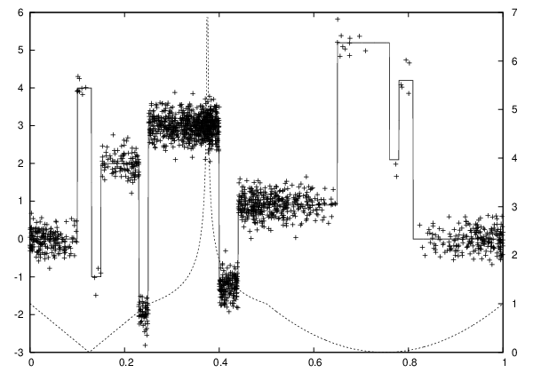
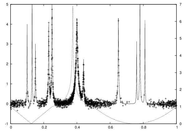
Note that these estimates can be slightly improved with case by case tuned parameters: for instance, for the first dataset (blocks), the choice κ=0\kappa=0 gives a slightly better looking estimate (the target function is constant by parts). In figure 3 we show datasets with the same signal-to-noise ratio and sample size as in figure 1 but the design is non-uniform (we plot the design density on each of them). We show the estimates based on these datasets in figure 4. The same parameters as for figure 2 are used.
Refer to caption
Refer to caption
Refer to caption
Refer to caption
Figure 3. Blocks, bumps, heavysine and doppler with Gaussian noise and non-uniform design.
Refer to caption
Refer to caption
Refer to caption
Refer to caption
Figure 4. Estimates based on the datasets in figure 3.

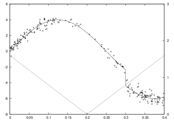
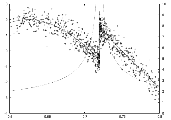
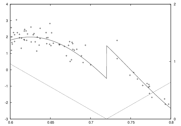
In figures 5 and 6 we give a more localised illustration of the heavysine dataset. We keep the same signal-to-noise ratio and sample size. We consider the design density

(5.1) μ⁡(x)=β+1x0β+1+(1−x0)β+1​|x−x0|β​𝟏[0,1]​(x),\mu(x)=\frac{\beta+1}{x_{0}^{\beta+1}+(1-x_{0})^{\beta+1}}\bigl|x-x_{0}\bigr|^{\beta}\mathbf{1}_{[0,1]}(x),

for x0=0.2,0.72x_{0}=0.2,0.72 and β=−0.5,1\beta=-0.5,1.

Refer to caption
Refer to caption
Refer to caption
Refer to caption
Figure 5. Heavysine datasets and estimates with design density (5.1) with x0=0.2x_{0}=0.2 and β=−0.5\beta=-0.5 at top, β=1\beta=1 at bottom.
Refer to caption
Refer to caption
Refer to caption
Refer to caption
Figure 6. Heavysine datasets and estimates with design density (5.1) with x0=0.72x_{0}=0.72 and β=−0.5\beta=-0.5 at top, β=1\beta=1 at bottom.

6. Discussion

6.1. On the procedure

  • •

    It is important to note that on the event Ωh\Omega_{h} the estimator f^h,κ\widehat{f}_{h,\kappa} is equal to the classical local polynomial estimator defined by

    (6.1) f^h,κ=arg⁡ming∈Vκ⁡‖g−Y‖h2,\widehat{f}_{h,\kappa}=\arg\min_{\displaystyle g\in V_{\kappa}}\|g-Y\|_{h}^{2},

    where Vκ=Span​{(ϕj)j=0,…,κ}V_{\kappa}=\text{Span}\{(\phi_{j})_{j=0,\ldots,\kappa}\}. A necessary condition for f^h,κ\widehat{f}_{h,\kappa} to minimise (6.1) is to be solution of the linear problem

    (6.2) find ​f^∈Vκ​ such that ​∀ϕ∈Vκ,⟨f^,ϕ⟩h=⟨Y,ϕ⟩h.\text{find }\widehat{f}\in V_{\kappa}\text{ such that }\forall\phi\in V_{\kappa},\quad\langle\widehat{f}\,,\,\phi\rangle_{h}=\langle Y\,,\,\phi\rangle_{h}.

    The main idea of the procedure is the following: if hh is a good bandwidth, then for any h′⩽hh^{\prime}\leqslant h and for all ϕ∈Vκ\phi\in V_{\kappa} we should have in view of (6.2):

    ⟨f^h−f^h′,ϕ⟩h′=⟨f^h−Y,ϕ⟩h′≈⟨ξ,ϕ⟩h′,\langle\widehat{f}_{h}-\widehat{f}_{h^{\prime}}\,,\,\phi\rangle_{h^{\prime}}=\langle\widehat{f}_{h}-Y\,,\,\phi\rangle_{h^{\prime}}\approx\langle\xi\,,\,\phi\rangle_{h^{\prime}},

    which means that the difference f^h−f^h′\widehat{f}_{h}-\widehat{f}_{h^{\prime}} is mainly noise, in the sense that σ−1​‖ϕ‖h′−1​⟨f^h−f^h′,ϕ⟩h′\sigma^{-1}\|\phi\|_{h^{\prime}}^{-1}\langle\widehat{f}_{h}-\widehat{f}_{h^{\prime}}\,,\,\phi\rangle_{h^{\prime}} is close in law to a standard Gaussian.

  • •

    The procedure (2.3) looks like the Lepski procedure: in a model where the estimators can be well sorted by their respective variances (this is the case with kernel estimators in the white noise model, see Lepski and Spokoiny (1997)), the Lepski procedure selects the largest bandwidth such that the corresponding estimator does not differ significantly from estimators with a smaller bandwidth. Here the idea is the same, but the proposed procedure is additionally sensitive to the design.

  • •

    The estimator f^n​(x0)\widehat{f}_{n}(x_{0}) only depends on κ\kappa and on the grid ℋ\mathcal{H} (to be chosen by the statistician). It does not depend on the regularity of ff nor any assumption on μ\mu. In this sense, this estimator is adaptive in both regularity and design.

  • •

    Note that 𝐗h=𝐅ht​𝐅h\mathbf{X}_{h}={}^{t}\mathbf{F}_{h}\mathbf{F}_{h} where 𝐅h\mathbf{F}_{h} is the matrix of size n×(κ+1)n\times(\kappa+1) with entries (𝐅h)i,j=(Xi−x0)j(\mathbf{F}_{h})_{i,j}=(X_{i}-x_{0})^{j} for 0⩽i⩽n0\leqslant i\leqslant n and 0⩽j⩽κ0\leqslant j\leqslant\kappa, and that ker⁡𝐗h=ker⁡𝐅h\ker{\mathbf{X}_{h}}=\ker{\mathbf{F}_{h}}. Thus when n<κ+1n<\kappa+1, 𝐗h\mathbf{X}_{h} is not invertible since its kernel is not zero, and Ωh=∅\Omega_{h}=\emptyset. This is the reason why theorem 1 is stated for n⩾κ+1n\geqslant\kappa+1 and in the step 33 of the procedure (see section 5.1) we must take m⩾κ+1m\geqslant\kappa+1 so that each interval in 𝒢\mathcal{G} contains at least κ+1\kappa+1 observations XiX_{i}.

  • •

    The reason why we need to take the grid ℋ=ℋ1arith\mathcal{H}=\mathcal{H}_{1}^{\textup{arith}} in theorem 2 is linked with the control of λn,ω\lambda_{n,\omega}. We can prove the theorem with a geometrical grid if we additionally assume λn,ω>λ\lambda_{n,\omega}>\lambda for λ>0\lambda>0, but we preferred to work only under the regularly varying design assumption with a restricted grid choice without extra assumption on the model.

  • •

    The fact that the noise level σ\sigma is known is of little importance. If it is unknown we can plug-in some estimator σ^n2\widehat{\sigma}_{n}^{2} in place of σ2\sigma^{2}. Following Gasser et al. (1986) or Buckley et al. (1988) we can consider

    (6.3) σ^n2=12​(n−1)​∑i=1n−1(Y(i+1)−Y(i))2,\widehat{\sigma}_{n}^{2}=\frac{1}{2(n-1)}\sum_{i=1}^{n-1}(Y_{(i+1)}-Y_{(i)})^{2},

    where Y(i)Y_{(i)} is the observation at the point X(i)X_{(i)} where X(1)⩽X(2)⩽…⩽X(n)X_{(1)}\leqslant X_{(2)}\leqslant\ldots\leqslant X_{(n)}.

6.2. Comparison with previous results

  • •

    In Guerre (1999), for the estimation of the regression function at the point 00 in a more general setup for the design, the author works conditionally on 𝔛n\mathfrak{X}_{n} and gives an upper bound with a data-driven rate similar to (3.4). The author considers then as an example the case of an i.i.d. design with density μ\mu such that μ⁡(x)∼xβ\mu(x)\sim x^{\beta} close to 00 for β>−1\beta>-1, which is a particular case of regularly varying density at 00 of index β\beta. Here the approach is the same: under the regular variation assumption we derive from theorem 1 an asymptotic upper-bound with a deterministic rate (theorem 2).

  • •

    Bandwidth selection procedures in local polynomial estimation can be found in Fan and Gijbels (1995), Goldenshluger and Nemirovski (1997) or Spokoiny (1998). In this last paper the author is interested in the regression function estimation near a change point. The main idea and difference between the work by Spokoiny (1998) and the previous work by Goldenshluger and Nemirovski (1997) is to solve the linear problem (6.2) in a non symmetrical neighbourhood of x0x_{0} not containing the change point. Our adaptive procedure (2.3) is mainly inspired from the work of Spokoiny and adapted for the degenerate random design problem. We have also made improvements, for instance we do not need to bound the estimator and the function at x0x_{0} by some known constant.

7. Proofs

In the following we denote by 𝐏k,h\mathbf{P}_{k,h} the projection in the space VkV_{k} for the scalar product ⟨⋅,⋅⟩h\langle\cdot\,,\,\cdot\rangle_{h}. We denote respectively by ⟨⋅,⋅⟩\langle\cdot\,,\,\cdot\rangle and by ∥⋅∥\|\cdot\| the Euclidean scalar product and the Euclidean norm in ℝκ+1\mathbb{R}^{\kappa+1}. We denote by ∥⋅∥∞\|\cdot\|_{\infty} the sup norm in ℝκ+1\mathbb{R}^{\kappa+1}. We define e1≜(1,0,…,0)e_{1}\triangleq(1,0,\ldots,0), the first canonical basis vector in ℝκ+1\mathbb{R}^{\kappa+1}.

7.1. Preparatory results and proof of theorem 1

The next lemma is a version of the local polynomial estimator bias-variance decomposition, which is classical: see Cleveland (1979), Tsybakov (1986), Korostelev and Tsybakov (1993), Fan and Gijbels (1995, 1996), Goldenshluger and Nemirovski (1997), Spokoiny (1998) and Tsybakov (2003), among others. The version given by lemma 1 is close to the one in Spokoiny (1998). Let us introduce for any positive integer kk the continuity modulus

ωf,k​(x0,h)=infP∈𝒫ksup|x−x0|⩽h|f⁡(x)−P⁡(x−x0)|.\omega_{f,k}(x_{0},h)=\inf_{P\in\mathcal{P}_{k}}\sup_{|x-x_{0}|\leqslant h}|f(x)-P(x-x_{0})|.

Note that if k1⩽k2k_{1}\leqslant k_{2} we clearly have ωf,k2​(x0,h)⩽ωf,k1​(x0,h)\omega_{f,k_{2}}(x_{0},h)\leqslant\omega_{f,k_{1}}(x_{0},h).

Lemma 1 (Bias variance decomposition).

On the event Ωh\Omega_{h} the estimator f^h,κ\widehat{f}_{h,\kappa} from definition 1 satisfies for any k⩽κk\leqslant\kappa

(7.1) |f^h(x0)−f(x0)|⩽λ−1(𝒢h)κ+1(ωf,k(x0,h)+σNn,h−1/2|γh|),|\widehat{f}_{h}(x_{0})-f(x_{0})|\leqslant\lambda^{-1}(\mathcal{G}_{h})\sqrt{\kappa+1}\bigl(\omega_{f,k}(x_{0},h)+\sigma N_{n,h}^{-1/2}|\gamma_{h}|\bigr),

where γh\gamma_{h} is, conditional on 𝔛n\mathfrak{X}_{n}, centered Gaussian such that 𝔼f,μn​{γh2|𝔛n}⩽1\mathbb{E}_{\,f,\mu}^{\,n}\{\gamma_{h}^{2}|\mathfrak{X}_{n}\}\leqslant 1.

Proof.

On Ωh\Omega_{h} we have 𝐗~h=𝐗h\widetilde{\mathbf{X}}_{h}=\mathbf{X}_{h} and λ(𝐗h)>Nn,h−1/2>0\lambda(\mathbf{X}_{h})>N_{n,h}^{-1/2}>0, then 𝐗h\mathbf{X}_{h} is invertible. Since Λh\Lambda_{h} is clearly invertible on this event, 𝒢h\mathcal{G}_{h} is also invertible. Let 0<ε⩽120<\varepsilon\leqslant\frac{1}{2}. By definition of ωf,κ​(x0,h)\omega_{f,\kappa}(x_{0},h) we can find a polynomial Pf,hε∈𝒫κP_{f,h}^{\varepsilon}\in\mathcal{P}_{\kappa} such that

supx∈[x0−h,x0+h]|f⁡(x)−Pf,hε​(x)|⩽ωf,κ​(x0,h)+εn.\sup_{x\in[x_{0}-h,x_{0}+h]}|f(x)-P_{f,h}^{\varepsilon}(x)|\leqslant\omega_{f,\kappa}(x_{0},h)+\frac{\varepsilon}{\sqrt{n}}.

In particular we have |f⁡(x0)−Pf,hε​(x0)|⩽εn|f(x_{0})-P_{f,h}^{\varepsilon}(x_{0})|\leqslant\frac{\varepsilon}{\sqrt{n}} and if we denote by θh\theta_{h} the coefficients vector of Pf,hεP_{f,h}^{\varepsilon} then

|f^h,κ​(x0)−f⁡(x0)|⩽|⟨Λh−1​(θ^h−θh),e1⟩|+εn=|⟨𝒢h−1​Λh​𝐗h​(θ^h−θh),e1⟩|+εn.|\widehat{f}_{h,\kappa}(x_{0})-f(x_{0})|\leqslant|\langle\Lambda_{h}^{-1}(\widehat{\theta}_{h}-\theta_{h})\,,\,e_{1}\rangle|+\frac{\varepsilon}{\sqrt{n}}=|\langle\mathcal{G}_{h}^{-1}\Lambda_{h}\mathbf{X}_{h}(\widehat{\theta}_{h}-\theta_{h})\,,\,e_{1}\rangle|+\frac{\varepsilon}{\sqrt{n}}.

Then in view of (6.2) one has for j=0,…,κj=0,\ldots,\kappa:

(𝐗h​(θ^h−θh))j=⟨f^h,κ−Pf,hε,ϕj⟩h=⟨Y−Pf,hε,ϕj⟩h=⟨f−Pf,hε,ϕj⟩h+⟨ξ,ϕj⟩h,\displaystyle(\mathbf{X}_{h}(\widehat{\theta}_{h}-\theta_{h}))_{j}=\langle\widehat{f}_{h,\kappa}-P_{f,h}^{\varepsilon}\,,\,\phi_{j}\rangle_{h}=\langle Y-P_{f,h}^{\varepsilon}\,,\,\phi_{j}\rangle_{h}=\langle f-P_{f,h}^{\varepsilon}\,,\,\phi_{j}\rangle_{h}+\langle\xi\,,\,\phi_{j}\rangle_{h},

thus we can decompose 𝐗h​(θ^h−θh)≜Bh+Vh\mathbf{X}_{h}(\widehat{\theta}_{h}-\theta_{h})\triangleq B_{h}+V_{h} and then:

|f^h,κ​(x0)−f⁡(x0)|⩽|⟨𝒢h−1​Λh​Bh,e1⟩|+|⟨𝒢h−1​Λh​Vh,e1⟩|+εn≜A+B+εn.|\widehat{f}_{h,\kappa}(x_{0})-f(x_{0})|\leqslant|\langle\mathcal{G}_{h}^{-1}\Lambda_{h}B_{h}\,,\,e_{1}\rangle|+|\langle\mathcal{G}_{h}^{-1}\Lambda_{h}V_{h}\,,\,e_{1}\rangle|+\frac{\varepsilon}{\sqrt{n}}\triangleq A+B+\frac{\varepsilon}{\sqrt{n}}.

We have

A\displaystyle A ⩽‖𝒢h−1​Λh​Bh‖⩽‖𝒢h−1‖|Λh​Bh|⩽‖𝒢h−1‖​κ+1​‖Λh​Bh‖∞,\displaystyle\leqslant\|\mathcal{G}_{h}^{-1}\Lambda_{h}B_{h}\|\leqslant\|\mathcal{G}_{h}^{-1}\|\|\Lambda_{h}B_{h}\|\leqslant\|\mathcal{G}_{h}^{-1}\|\sqrt{\kappa+1}\|\Lambda_{h}B_{h}\|_{\infty},

and

|(Λh​Bh)j|=‖ϕj‖h−1​|⟨f−Pf,hε,ϕj⟩h|⩽‖f−Pf,hε‖h⩽ωf,κ​(x0,h)+εn.|(\Lambda_{h}B_{h})_{j}|=\|\phi_{j}\|_{h}^{-1}|\langle f-P_{f,h}^{\varepsilon}\,,\,\phi_{j}\rangle_{h}|\leqslant\|f-P_{f,h}^{\varepsilon}\|_{h}\leqslant\omega_{f,\kappa}(x_{0},h)+\frac{\varepsilon}{\sqrt{n}}.

For any symmetrical and positive matrix MM we have λ−1​(M)=‖M−1‖\lambda^{-1}(M)=\|M^{-1}\| then since ‖Λh−1‖⩽1\|\Lambda_{h}^{-1}\|\leqslant 1 we have on the event Ωh\Omega_{h}:

‖𝒢h−1‖=‖Λh−1​𝐗h−1​Λh−1‖⩽‖𝐗h−1‖=λ−1​(𝐗h)⩽Nn,h1/2⩽n.\|\mathcal{G}_{h}^{-1}\|=\|\Lambda_{h}^{-1}\mathbf{X}_{h}^{-1}\Lambda_{h}^{-1}\|\leqslant\|\mathbf{X}_{h}^{-1}\|=\lambda^{-1}(\mathbf{X}_{h})\leqslant N_{n,h}^{1/2}\leqslant\sqrt{n}.

Thus A⩽‖𝒢h−1‖​κ+1​ωf,κ​(x0,h)+ε​κ+1⩽‖𝒢h−1‖​κ+1​ωf,k​(x0,h)+ε​κ+1A\leqslant\|\mathcal{G}_{h}^{-1}\|\sqrt{\kappa+1}\omega_{f,\kappa}(x_{0},h)+\varepsilon\sqrt{\kappa+1}\leqslant\|\mathcal{G}_{h}^{-1}\|\sqrt{\kappa+1}\omega_{f,k}(x_{0},h)+\varepsilon\sqrt{\kappa+1} since k⩽κk\leqslant\kappa. Conditional on 𝔛n\mathfrak{X}_{n}, the random vector VhV_{h} is centered Gaussian with covariance matrix σ2​Nn,h−1​𝐗h\sigma^{2}N_{n,h}^{-1}\mathbf{X}_{h}. Thus 𝒢h−1​Λh​Vh\mathcal{G}_{h}^{-1}\Lambda_{h}V_{h} is again centered Gaussian, with covariance matrix

σ2​Nn,h−1​𝒢h−1​Λh​𝐗h​Λh​𝒢h−1=σ2​Nn,h−1​𝒢h−1,\sigma^{2}N_{n,h}^{-1}\mathcal{G}_{h}^{-1}\Lambda_{h}\mathbf{X}_{h}\Lambda_{h}\mathcal{G}_{h}^{-1}=\sigma^{2}N_{n,h}^{-1}\mathcal{G}_{h}^{-1},

and BB is then centered Gaussian with variance

σ2​Nn,h−1​⟨e1,𝒢h−1​e1⟩⩽σ2​Nn,h−1​‖𝒢h−1‖.\sigma^{2}N_{n,h}^{-1}\langle e_{1}\,,\,\mathcal{G}_{h}^{-1}e_{1}\rangle\leqslant\sigma^{2}N_{n,h}^{-1}\|\mathcal{G}_{h}^{-1}\|.

Since 𝒢h\mathcal{G}_{h} is positive symmetrical and its entries are smaller than one in absolute value we get ‖𝒢−1‖=λ−1​(𝒢h)\|\mathcal{G}^{-1}\|=\lambda^{-1}(\mathcal{G}_{h}) and λ⁡(𝒢h)=inf‖x‖=1⟨x,𝒢h​x⟩⩽‖𝒢h​e1‖⩽κ+1\lambda(\mathcal{G}_{h})=\inf_{\|x\|=1}\langle x\,,\,\mathcal{G}_{h}x\rangle\leqslant\|\mathcal{G}_{h}e_{1}\|\leqslant\sqrt{\kappa+1}. Thus ‖𝒢h−1‖⩽κ+1​‖𝒢h−1‖2\|\mathcal{G}_{h}^{-1}\|\leqslant\sqrt{\kappa+1}\|\mathcal{G}_{h}^{-1}\|^{2}, and the proposition follows. ∎

Let us introduce the events

𝒜h′,h,j≜{|⟨f^h,κ−f^h′,κ,ϕj⟩h′|⩽σ∥ϕj∥h′Tn,h′,h},\mathcal{A}_{h^{\prime},h,j}\triangleq\bigl\{|\langle\widehat{f}_{h,\kappa}-\widehat{f}_{h^{\prime},\kappa}\,,\,\phi_{j}\rangle_{h^{\prime}}|\leqslant\sigma\|\phi_{j}\|_{h^{\prime}}T_{n,h^{\prime},h}\bigr\},

𝒜h′,h≜⋂j=0κ𝒜h′,h,j\mathcal{A}_{h^{\prime},h}\triangleq\bigcap_{j=0}^{\kappa}\mathcal{A}_{h^{\prime},h,j} and 𝒜h≜⋂h′∈ℋh𝒜h′,h\mathcal{A}_{h}\triangleq\bigcap_{h^{\prime}\in\mathcal{H}_{h}}\mathcal{A}_{h^{\prime},h}. The following lemma shows that if some bandwidth hh is good in the sense that h⩽Hn,ωh\leqslant H_{n,\omega} (hh is smaller than the ideal adaptive bandwidth) then hh can be selected by the procedure with a large probability.

Lemma 2.

Let f∈ℱδ​(x0,ω)f\in\mathcal{F}_{\delta}(x_{0},\omega) for ω∈RV⁡(s)\omega\in\mathrm{RV}(s) with 0<s⩽κ+10<s\leqslant\kappa+1. If hh is such that h⩽Hn,ω∧δh\leqslant H_{n,\omega}\wedge\delta we have on Ωh\Omega_{h} for any n⩾κ+1n\geqslant\kappa+1:

ℙf,μn​{𝒜h|𝔛n}⩾1−(κ+1)​Nn,h−2​p.\mathbb{P}_{f,\mu}^{n}\bigl\{\mathcal{A}_{h}|\mathfrak{X}_{n}\bigr\}\geqslant 1-(\kappa+1)N_{n,h}^{-2p}.
Proof.

Let j∈{0,…,κ}j\in\{0,\ldots,\kappa\} and h′∈ℋhh^{\prime}\in\mathcal{H}_{h}. On Ωh\Omega_{h} we have in view of (6.1) that f^h,κ=𝐏κ,h​(Y)\widehat{f}_{h,\kappa}=\mathbf{P}_{\kappa,h}(Y) thus using (6.2) we can decompose:

⟨f^h′,κ−f^h,κ,ϕj⟩h′=⟨Y−f^h,κ,ϕj⟩h′\displaystyle\langle\widehat{f}_{h^{\prime},\kappa}-\widehat{f}_{h,\kappa}\,,\,\phi_{j}\rangle_{h^{\prime}}=\langle Y-\widehat{f}_{h,\kappa}\,,\,\phi_{j}\rangle_{h^{\prime}} =⟨f−f^h,κ,ϕj⟩h′+⟨ξ,ϕj⟩h′\displaystyle=\langle f-\widehat{f}_{h,\kappa}\,,\,\phi_{j}\rangle_{h^{\prime}}+\langle\xi\,,\,\phi_{j}\rangle_{h^{\prime}}
=⟨f−𝐏κ,h​(f),ϕj⟩h′+⟨𝐏κ,h​(f)−f^h,κ,ϕj⟩h′+⟨ξ,ϕj⟩h′\displaystyle=\langle f-\mathbf{P}_{\kappa,h}(f)\,,\,\phi_{j}\rangle_{h^{\prime}}+\langle\mathbf{P}_{\kappa,h}(f)-\widehat{f}_{h,\kappa}\,,\,\phi_{j}\rangle_{h^{\prime}}+\langle\xi\,,\,\phi_{j}\rangle_{h^{\prime}}
=⟨f−𝐏κ,h​(f),ϕj⟩h′+⟨𝐏κ,h​(f−Y),ϕj⟩h′+⟨ξ,ϕj⟩h′\displaystyle=\langle f-\mathbf{P}_{\kappa,h}(f)\,,\,\phi_{j}\rangle_{h^{\prime}}+\langle\mathbf{P}_{\kappa,h}(f-Y)\,,\,\phi_{j}\rangle_{h^{\prime}}+\langle\xi\,,\,\phi_{j}\rangle_{h^{\prime}}
=⟨f−𝐏κ,h​(f),ϕj⟩h′−⟨𝐏κ,h​(ξ),ϕj⟩h′+⟨ξ,ϕj⟩h′\displaystyle=\langle f-\mathbf{P}_{\kappa,h}(f)\,,\,\phi_{j}\rangle_{h^{\prime}}-\langle\mathbf{P}_{\kappa,h}(\xi)\,,\,\phi_{j}\rangle_{h^{\prime}}+\langle\xi\,,\,\phi_{j}\rangle_{h^{\prime}}
≜A+B+C.\displaystyle\triangleq A+B+C.

The term AA is a bias term. By the definition of ωf,k​(x0,h)\omega_{f,k}(x_{0},h) we can find a polynomial Pf,hn∈VkP_{f,h}^{n}\in V_{k} such that

supx∈[x0−h,x0+h]|f⁡(x)−Pf,hn​(x)|⩽ωf,k​(x0,h)+εn,\sup_{x\in[x_{0}-h,x_{0}+h]}|f(x)-P_{f,h}^{n}(x)|\leqslant\omega_{f,k}(x_{0},h)+\varepsilon_{n},

where εn≜Cκ​σ2​Cp​log⁡2n\varepsilon_{n}\triangleq\frac{C_{\kappa}\sigma}{2}\sqrt{\frac{C_{p}\log 2}{n}} (see (2.4)). Since h′⩽h⩽δh^{\prime}\leqslant h\leqslant\delta, f∈ℱδ​(x0,ω)f\in\mathcal{F}_{\delta}(x_{0},\omega) and Pf,hn∈Vk⊂VκP_{f,h}^{n}\in V_{k}\subset V_{\kappa} we get

|A|⩽‖f−𝐏κ,h​(f)‖h′​‖ϕj‖h′\displaystyle|A|\leqslant\|f-\mathbf{P}_{\kappa,h}(f)\|_{h^{\prime}}\|\phi_{j}\|_{h^{\prime}} ⩽‖f−Pf,hn−𝐏κ,h​(f−Pf,hn)‖h​‖ϕj‖h′\displaystyle\leqslant\|f-P_{f,h}^{n}-\mathbf{P}_{\kappa,h}(f-P_{f,h}^{n})\|_{h}\|\phi_{j}\|_{h^{\prime}}
⩽‖f−Pf,hn‖h​‖ϕj‖h′\displaystyle\leqslant\|f-P_{f,h}^{n}\|_{h}\|\phi_{j}\|_{h^{\prime}}
⩽‖ϕj‖h′​(ωf,k​(x0,h)+εn)⩽‖ϕj‖h′​(ω⁡(h)+εn),\displaystyle\leqslant\|\phi_{j}\|_{h^{\prime}}(\omega_{f,k}(x_{0},h)+\varepsilon_{n})\leqslant\|\phi_{j}\|_{h^{\prime}}(\omega(h)+\varepsilon_{n}),

since 𝐏κ,h\mathbf{P}_{\kappa,h} is a projection with respect to ⟨⋅,⋅⟩h\langle\cdot\,,\,\cdot\rangle_{h}. If h<Hn,ωh<H_{n,\omega} we have in view of (3.3) that ω⁡(h)⩽σ​Nn,h−1​log⁡n\omega(h)\leqslant\sigma\sqrt{N_{n,h}^{-1}\log n}. When h=Hn,ωh=H_{n,\omega} two cases can occur. If the graphs of h↦σ​Nn,h−1​log⁡nh\mapsto\sigma\sqrt{N_{n,h}^{-1}\log n} and h↦ω⁡(h)h\mapsto\omega(h) cross each other we have ω⁡(h)=σ​Nn,h−1​log⁡n\omega(h)=\sigma\sqrt{N_{n,h}^{-1}\log n}. When these graphs do not cross we introduce Hn,ω−=max⁡{h∈ℋ|h<Hn,ω}H_{n,\omega}^{-}=\max\{h\in\mathcal{H}|h<H_{n,\omega}\} and Hn,ω+=min⁡{h∈ℋ|h⩾Hn,ω}H_{n,\omega}^{+}=\min\{h\in\mathcal{H}|h\geqslant H_{n,\omega}\}. If ℋ=ℋaarith\mathcal{H}=\mathcal{H}_{a}^{\textup{arith}} we have Nn,Hn,ω⩽Nn,Hn,ω+⩽Nn,Hn,ω−+aN_{n,H_{n,\omega}}\leqslant N_{n,H_{n,\omega}^{+}}\leqslant N_{n,H_{n,\omega}^{-}}+a while when ℋ=ℋageom\mathcal{H}=\mathcal{H}_{a}^{\textup{geom}} we get Nn,Hn,ω⩽Nn,Hn,ω+⩽(1+a)​Nn,Hn,ω−N_{n,H_{n,\omega}}\leqslant N_{n,H_{n,\omega}^{+}}\leqslant(1+a)N_{n,H_{n,\omega}^{-}}. Then for any h⩽Hn,ωh\leqslant H_{n,\omega}:

(7.2) |A|⩽{‖ϕj‖h′​(σ​(Nn,h−a)−1​log⁡n+εn) if ​ℋ=ℋaarith,‖ϕj‖h′​(σ​(1+a)​Nn,h−1​log⁡n+εn) if ​ℋ=ℋageom.|A|\leqslant\begin{cases}\|\phi_{j}\|_{h^{\prime}}(\sigma\sqrt{(N_{n,h}-a)^{-1}\log n}+\varepsilon_{n})&\text{ if }\mathcal{H}=\mathcal{H}_{a}^{\textup{arith}},\\ \|\phi_{j}\|_{h^{\prime}}(\sigma\sqrt{(1+a)N_{n,h}^{-1}\log n}+\varepsilon_{n})&\text{ if }\mathcal{H}=\mathcal{H}_{a}^{\textup{geom}}.\end{cases}

Conditional on 𝔛n\mathfrak{X}_{n}, BB and CC are centered Gaussian. We have ℒ⁡(C|𝔛n)=𝒩⁡(0,σ2​Nn,h′−1​‖ϕj‖h′2)\mathcal{L}(C|\mathfrak{X}_{n})=\mathcal{N}(0,\sigma^{2}N_{n,h^{\prime}}^{-1}\|\phi_{j}\|_{h^{\prime}}^{2}) and conditional on 𝔛n\mathfrak{X}_{n} the vector 𝐏κ,h​(ξ)\mathbf{P}_{\kappa,h}(\xi) is centered Gaussian with covariance matrix

σ2​𝐏κ,h​𝐏κ,ht=σ2​𝐏κ,h,\sigma^{2}\mathbf{P}_{\kappa,h}{}^{t}\mathbf{P}_{\kappa,h}=\sigma^{2}\mathbf{P}_{\kappa,h},

since 𝐏κ,h\mathbf{P}_{\kappa,h} is a projection. Thus BB is centered Gaussian with variance

𝔼f,μn​{⟨𝐏κ,h​(ξ),ϕj⟩h′2|𝔛n}\displaystyle\mathbb{E}_{\,f,\mu}^{\,n}\{\langle\mathbf{P}_{\kappa,h}(\xi)\,,\,\phi_{j}\rangle_{h^{\prime}}^{2}|\mathfrak{X}_{n}\} ⩽‖ϕj‖h′2​𝔼f,μn​{‖𝐏κ,h​(ξ)‖h′2|𝔛n}\displaystyle\leqslant\|\phi_{j}\|_{h^{\prime}}^{2}\mathbb{E}_{\,f,\mu}^{\,n}\{\|\mathbf{P}_{\kappa,h}(\xi)\|_{h^{\prime}}^{2}|\mathfrak{X}_{n}\}
=Nn,h′−1​‖ϕj‖h′2​tr​(𝕍​ar​(𝐏κ,h​(ξ)|𝔛n))\displaystyle=N_{n,h^{\prime}}^{-1}\|\phi_{j}\|_{h^{\prime}}^{2}\text{tr}(\mathbb{V}\text{ar}(\mathbf{P}_{\kappa,h}(\xi)|\mathfrak{X}_{n}))
=σ2​Nn,h′−1​‖ϕj‖h′2​tr​(𝐏κ,h)\displaystyle=\sigma^{2}N_{n,h^{\prime}}^{-1}\|\phi_{j}\|_{h^{\prime}}^{2}\text{tr}(\mathbf{P}_{\kappa,h})
⩽σ2​Nn,h′−1​‖ϕj‖h′2​dim(Vκ)⩽σ2​Nn,h′−1​‖ϕj‖h′2​(κ+1),\displaystyle\leqslant\sigma^{2}N_{n,h^{\prime}}^{-1}\|\phi_{j}\|_{h^{\prime}}^{2}\dim(V_{\kappa})\leqslant\sigma^{2}N_{n,h^{\prime}}^{-1}\|\phi_{j}\|_{h^{\prime}}^{2}(\kappa+1),

where we last used that 𝐏κ,h\mathbf{P}_{\kappa,h} is the projection in VκV_{\kappa}. Then conditional on 𝔛n\mathfrak{X}_{n}, B+CB+C is centered Gaussian with variance

𝔼f,μn​{(B+C)2|𝔛n}\displaystyle\mathbb{E}_{\,f,\mu}^{\,n}\{(B+C)^{2}|\mathfrak{X}_{n}\} ⩽𝔼f,μn​{B2+2​B​C+C2|𝔛n}\displaystyle\leqslant\mathbb{E}_{\,f,\mu}^{\,n}\{B^{2}+2BC+C^{2}|\mathfrak{X}_{n}\}
⩽𝔼f,μn​{B2|𝔛n}+2​𝔼f,μn​{B2|𝔛n}​𝔼f,μn​{C2|𝔛n}+𝔼f,μn​{C2|𝔛n}\displaystyle\leqslant\mathbb{E}_{\,f,\mu}^{\,n}\{B^{2}|\mathfrak{X}_{n}\}+2\sqrt{\mathbb{E}_{\,f,\mu}^{\,n}\{B^{2}|\mathfrak{X}_{n}\}\mathbb{E}_{\,f,\mu}^{\,n}\{C^{2}|\mathfrak{X}_{n}\}}+\mathbb{E}_{\,f,\mu}^{\,n}\{C^{2}|\mathfrak{X}_{n}\}
⩽σ2​(1+κ+1)2​Nn,h′−1​‖ϕj‖h′2​Cκ2.\displaystyle\leqslant\sigma^{2}(1+\sqrt{\kappa+1})^{2}N_{n,h^{\prime}}^{-1}\|\phi_{j}\|_{h^{\prime}}^{2}C_{\kappa}^{2}.

Using (7.2) and since 2⩽Nn,h⩽n2\leqslant N_{n,h}\leqslant n on Ωh\Omega_{h} we have

𝒜h′,h,jc⊂{|B+C|σNn,h′−1/2∥ϕj∥h′Cκ>Cp​log⁡Nn,h/2},\mathcal{A}_{h^{\prime},h,j}^{c}\subset\Bigl\{\frac{|B+C|}{\sigma N_{n,h^{\prime}}^{-1/2}\|\phi_{j}\|_{h^{\prime}}C_{\kappa}}>\sqrt{C_{p}\log N_{n,h}}/2\Bigr\},

and using a standard Gaussian large deviation inequality we get

ℙf,μn​{𝒜h′,h,jc|𝔛n}⩽exp⁡(−(1+2​p)​log⁡Nn,h)=Nn,h−(1+2​p).\displaystyle\mathbb{P}_{f,\mu}^{n}\bigl\{\mathcal{A}_{h^{\prime},h,j}^{c}\bigl|\mathfrak{X}_{n}\bigr\}\leqslant\exp\bigl(-(1+2p)\log N_{n,h}\bigr)=N_{n,h}^{-(1+2p)}.

Since #⁡(ℋh)⩽Nn,h\#(\mathcal{H}_{h})\leqslant N_{n,h} we finally have

ℙf,μn​{𝒜hc|𝔛n}⩽ℙf,μn​{⋃h′∈ℋh⋃j=0κ𝒜h′,h,jc|𝔛n}⩽(κ+1)​Nn,h−2​p.∎\mathbb{P}_{f,\mu}^{n}\{\mathcal{A}_{h}^{c}|\mathfrak{X}_{n}\}\leqslant\mathbb{P}_{f,\mu}^{n}\Bigl\{\bigcup_{h^{\prime}\in\mathcal{H}_{h}}\bigcup_{j=0}^{\kappa}\mathcal{A}_{h^{\prime},h,j}^{c}\bigl|\mathfrak{X}_{n}\Bigr\}\leqslant(\kappa+1)N_{n,h}^{-2p}.\qed
Lemma 3.

Let h∈ℋh\in\mathcal{H} and h′∈ℋhh^{\prime}\in\mathcal{H}_{h}. On the event Ωh′∩𝒜h′,h\Omega_{h^{\prime}}\cap\mathcal{A}_{h^{\prime},h} one has:

|f^h​(x0)−f^h′​(x0)|⩽Cp,κ,a​‖𝒢h′−1‖​σ​Nn,h′−1​log⁡n,|\widehat{f}_{h}(x_{0})-\widehat{f}_{h^{\prime}}(x_{0})|\leqslant C_{p,\kappa,a}\|\mathcal{G}_{h^{\prime}}^{-1}\|\sigma\sqrt{N_{n,h^{\prime}}^{-1}\log n},

where Cp,κ,a≜κ+1​(1+a+Cκ​Cp)C_{p,\kappa,a}\triangleq\sqrt{\kappa+1}(\sqrt{1+a}+C_{\kappa}\sqrt{C_{p}}).

Proof.

In view of definition 1 and since 𝒢h′\mathcal{G}_{h^{\prime}} is invertible on Ωh′\Omega_{h^{\prime}} we have

|f^h​(x0)−f^h′​(x0)|=|⟨Λh′−1​(θ^h−θ^h′),e1⟩|\displaystyle|\widehat{f}_{h}(x_{0})-\widehat{f}_{h^{\prime}}(x_{0})|=|\langle\Lambda_{h^{\prime}}^{-1}(\widehat{\theta}_{h}-\widehat{\theta}_{h^{\prime}})\,,\,e_{1}\rangle| ⩽‖Λh′−1​(θ^h−θ^h′)‖\displaystyle\leqslant\|\Lambda_{h^{\prime}}^{-1}(\widehat{\theta}_{h}-\widehat{\theta}_{h^{\prime}})\|
=‖𝒢h′−1​Λh′​𝐗h′​(θ^h−θ^h′)‖\displaystyle=\|\mathcal{G}_{h^{\prime}}^{-1}\Lambda_{h^{\prime}}\mathbf{X}_{h^{\prime}}(\widehat{\theta}_{h}-\widehat{\theta}_{h^{\prime}})\|
≜‖𝒢h′−1​Λh′​Dh′,h‖⩽‖𝒢h′−1‖​κ+1​‖Λh′​Dh′,h‖∞.\displaystyle\triangleq\|\mathcal{G}_{h^{\prime}}^{-1}\Lambda_{h^{\prime}}D_{h^{\prime},h}\|\leqslant\|\mathcal{G}_{h^{\prime}}^{-1}\|\sqrt{\kappa+1}\|\Lambda_{h^{\prime}}D_{h^{\prime},h}\|_{\infty}.

On 𝒜h′,h\mathcal{A}_{h^{\prime},h} we have for any j∈{0,…,κ}j\in\{0,\ldots,\kappa\}:

|(Dh′,h)j|=|⟨f^h−f^h′,ϕj⟩h′|⩽σ​‖ϕj‖h′​Tn,h′,h,|(D_{h^{\prime},h})_{j}|=|\langle\widehat{f}_{h}-\widehat{f}_{h^{\prime}}\,,\,\phi_{j}\rangle_{h^{\prime}}|\leqslant\sigma\|\phi_{j}\|_{h^{\prime}}T_{n,h^{\prime},h},

thus ‖Λh′​Dh′,h‖∞⩽σ​Tn,h′,h\|\Lambda_{h^{\prime}}D_{h^{\prime},h}\|_{\infty}\leqslant\sigma T_{n,h^{\prime},h}. Since h′⩽hh^{\prime}\leqslant h and Nn,h⩽nN_{n,h}\leqslant n we have when ℋ=ℋageom\mathcal{H}=\mathcal{H}_{a}^{\textup{geom}}

(7.3) Tn,h′,h⩽(Cκ​Cp+1+a)​Nn,h′​log⁡n,T_{n,h^{\prime},h}\leqslant(C_{\kappa}\sqrt{C_{p}}+\sqrt{1+a})\sqrt{N_{n,h^{\prime}}\log n},

and when ℋ=ℋaarith\mathcal{H}=\mathcal{H}_{a}^{\textup{arith}} we have by construction Nn,h⩾1+aN_{n,h}\geqslant 1+a thus (Nn,h−a)−1⩽(1+a)​Nn,h−1(N_{n,h}-a)^{-1}\leqslant(1+a)N_{n,h}^{-1} and (7.3) holds again. ∎

Lemma 4.

For any p,α>0p,\alpha>0 and 0<h′⩽h⩽10<h^{\prime}\leqslant h\leqslant 1 the estimator f^h′\widehat{f}_{h^{\prime}} given by definition 1 satisfies:

supf∈𝒰⁡(α)𝔼f,μn​{|f^h′​(x0)|p|𝔛n}⩽Cσ,p,κ​(α∨1)p​Nn,hp/2,\sup_{\displaystyle f\in\mathcal{U}(\alpha)}\mathbb{E}_{\,f,\mu}^{\,n}\bigl\{|\widehat{f}_{h^{\prime}}(x_{0})|^{p}|\mathfrak{X}_{n}\bigr\}\leqslant C_{\sigma,p,\kappa}(\alpha\vee 1)^{p}N_{n,h}^{p/2},

where Cσ,p,κ=(κ+1)p/22π∫ℝ+(1+σt)pexp(−t2/2)dtC_{\sigma,p,\kappa}=(\kappa+1)^{p/2}\sqrt{\frac{2}{\pi}}\int_{\mathbb{R}^{+}}(1+\sigma t)^{p}\exp(-t^{2}/2)dt.

Proof.

If Nn,h′=0N_{n,h^{\prime}}=0 we have f^h′=0\widehat{f}_{h^{\prime}}=0 and the result is obvious, thus we assume Nn,h′>0N_{n,h^{\prime}}>0. Since λ(𝐗~h′)⩾Nn,h′−1/2>0\lambda(\widetilde{\mathbf{X}}_{h^{\prime}})\geqslant N_{n,h^{\prime}}^{-1/2}>0, 𝐗~h′\widetilde{\mathbf{X}}_{h^{\prime}} and Λh′\Lambda_{h^{\prime}} are invertible and also 𝒢h′\mathcal{G}_{h^{\prime}}. Thus,

f^h′​(x0)=⟨Λh′−1​θ^h′,e1⟩=⟨𝒢h′−1​Λh′​𝐗~h′​θ^h′,e1⟩=⟨𝒢h′−1​Λh′​𝐘h′,e1⟩.\widehat{f}_{h^{\prime}}(x_{0})=\langle\Lambda_{h^{\prime}}^{-1}\widehat{\theta}_{h^{\prime}}\,,\,e_{1}\rangle=\langle\mathcal{G}_{h^{\prime}}^{-1}\Lambda_{h^{\prime}}\widetilde{\mathbf{X}}_{h^{\prime}}\widehat{\theta}_{h^{\prime}}\,,\,e_{1}\rangle=\langle\mathcal{G}_{h^{\prime}}^{-1}\Lambda_{h^{\prime}}\mathbf{Y}_{h^{\prime}}\,,\,e_{1}\rangle.

For any j∈{0,…,κ}j\in\{0,\ldots,\kappa\} we have (Λh′​𝐘h′)j=‖ϕj‖h′−1​(⟨f,ϕj⟩h′+⟨ξ,ϕj⟩h′)≜Bh′,j+Vh′,j(\Lambda_{h^{\prime}}\mathbf{Y}_{h^{\prime}})_{j}=\|\phi_{j}\|_{h^{\prime}}^{-1}(\langle f\,,\,\phi_{j}\rangle_{h^{\prime}}+\langle\xi\,,\,\phi_{j}\rangle_{h^{\prime}})\triangleq B_{h^{\prime},j}+V_{h^{\prime},j}. Since f∈𝒰⁡(α)f\in\mathcal{U}(\alpha) we have

|Bh′,j|⩽‖ϕj‖h′−1​|⟨f,ϕj⟩h′|⩽‖f‖h′⩽α,|B_{h^{\prime},j}|\leqslant\|\phi_{j}\|_{h^{\prime}}^{-1}|\langle f\,,\,\phi_{j}\rangle_{h^{\prime}}|\leqslant\|f\|_{h^{\prime}}\leqslant\alpha,

thus ‖Bh′‖∞⩽α\|B_{h^{\prime}}\|_{\infty}\leqslant\alpha. Since Vh′V_{h^{\prime}} is, conditional on 𝔛n\mathfrak{X}_{n}, a centered Gaussian vector with variance σ2​Nn,h′−1​Λh′​𝐗h′​Λh′\sigma^{2}N_{n,h^{\prime}}^{-1}\Lambda_{h^{\prime}}\mathbf{X}_{h^{\prime}}\Lambda_{h^{\prime}} we have that 𝒢h′−1​Λh′​Vh′\mathcal{G}_{h^{\prime}}^{-1}\Lambda_{h^{\prime}}V_{h^{\prime}} is also centered Gaussian, with variance

σ2​Nn,h′−1​𝒢h′−1​Λh′​𝐗h′​Λh′​𝒢h′−1=σ2​Nn,h′−1​Λh′−1​𝐗~h′−1​𝐗h′​𝐗~h′−1​Λh′−1.\sigma^{2}N_{n,h^{\prime}}^{-1}\mathcal{G}_{h^{\prime}}^{-1}\Lambda_{h^{\prime}}\mathbf{X}_{h^{\prime}}\Lambda_{h^{\prime}}\mathcal{G}_{h^{\prime}}^{-1}=\sigma^{2}N_{n,h^{\prime}}^{-1}\Lambda_{h^{\prime}}^{-1}\widetilde{\mathbf{X}}_{h^{\prime}}^{-1}\mathbf{X}_{h^{\prime}}\widetilde{\mathbf{X}}_{h^{\prime}}^{-1}\Lambda_{h^{\prime}}^{-1}.

The variable ⟨𝒢h′−1​Vh′,e1⟩\langle\mathcal{G}_{h^{\prime}}^{-1}V_{h^{\prime}}\,,\,e_{1}\rangle is then conditional on 𝔛n\mathfrak{X}_{n} centered Gaussian with variance

vh′2≜σ2​Nn,h′−1​⟨e1​Λh′−1​𝐗~h′−1​𝐗h′​𝐗~h′−1​Λh′−1,e1⟩⩽σ2​Nn,h′−1​‖Λh′−1‖2​‖𝐗~h′−1‖2​‖𝐗h′‖,v_{h^{\prime}}^{2}\triangleq\sigma^{2}N_{n,h^{\prime}}^{-1}\langle e_{1}\Lambda_{h^{\prime}}^{-1}\widetilde{\mathbf{X}}_{h^{\prime}}^{-1}\mathbf{X}_{h^{\prime}}\widetilde{\mathbf{X}}_{h^{\prime}}^{-1}\Lambda_{h^{\prime}}^{-1}\,,\,e_{1}\rangle\leqslant\sigma^{2}N_{n,h^{\prime}}^{-1}\|\Lambda_{h^{\prime}}^{-1}\|^{2}\|\widetilde{\mathbf{X}}_{h^{\prime}}^{-1}\|^{2}\|\mathbf{X}_{h^{\prime}}\|,

and since clearly ‖𝐗h′‖⩽κ+1\|\mathbf{X}_{h^{\prime}}\|\leqslant\kappa+1, ‖Λh′−1‖⩽1\|\Lambda_{h^{\prime}}^{-1}\|\leqslant 1 and ‖𝐗~h′−1‖=λ−1​(𝐗~h′)⩽Nn,h′1/2\|\widetilde{\mathbf{X}}_{h^{\prime}}^{-1}\|=\lambda^{-1}(\widetilde{\mathbf{X}}_{h^{\prime}})\leqslant N_{n,h^{\prime}}^{1/2} we have vh′2⩽σ2​(κ+1)v_{h^{\prime}}^{2}\leqslant\sigma^{2}(\kappa+1) and ‖𝒢h′−1‖⩽‖Λh′−1‖​‖𝐗~h′−1‖​‖Λh′−1‖⩽Nn,h′1/2\|\mathcal{G}_{h^{\prime}}^{-1}\|\leqslant\|\Lambda_{h^{\prime}}^{-1}\|\|\widetilde{\mathbf{X}}_{h^{\prime}}^{-1}\|\|\Lambda_{h^{\prime}}^{-1}\|\leqslant N_{n,h^{\prime}}^{1/2}. Finally we have

|f^h′​(x0)|⩽|⟨𝒢h′−1​Bh′,e1⟩|+|⟨𝒢h′−1​Vh′,e1⟩|\displaystyle|\widehat{f}_{h^{\prime}}(x_{0})|\leqslant|\langle\mathcal{G}_{h^{\prime}}^{-1}B_{h^{\prime}}\,,\,e_{1}\rangle|+|\langle\mathcal{G}_{h^{\prime}}^{-1}V_{h^{\prime}}\,,\,e_{1}\rangle| ⩽|𝒢h′−1|(‖Bh′‖+σ​κ+1​|γh′|)\displaystyle\leqslant\|\mathcal{G}_{h^{\prime}}^{-1}\|(\|B_{h^{\prime}}\|+\sigma\sqrt{\kappa+1}|\gamma_{h^{\prime}}|)
⩽κ+1​Nn,h′1/2​(‖Bh′‖∞+σ​|γh′|)\displaystyle\leqslant\sqrt{\kappa+1}N_{n,h^{\prime}}^{1/2}(\|B_{h^{\prime}}\|_{\infty}+\sigma|\gamma_{h^{\prime}}|)
⩽κ+1​(α∨1)​Nn,h1/2​(1+σ​|γh′|),\displaystyle\leqslant\sqrt{\kappa+1}(\alpha\vee 1)N_{n,h}^{1/2}(1+\sigma|\gamma_{h^{\prime}}|),

where γh′\gamma_{h^{\prime}} is, conditional on 𝔛n\mathfrak{X}_{n}, centered Gaussian with variance vh′2⩽1v_{h^{\prime}}^{2}\leqslant 1. The lemma follows by integrating with respect to ℙf,μn(⋅|𝔛n)\mathbb{P}_{f,\mu}^{n}(\cdot|\mathfrak{X}_{n}). ∎

Proof of theorem 1.

We first work on the event {H^n<Hn,ω∗}\{\widehat{H}_{n}<H_{n,\omega}^{*}\}. By definition of H^n\widehat{H}_{n} we have {H^n<Hn,ω∗}⊂𝒜Hn,ω∗c\{\widehat{H}_{n}<H_{n,\omega}^{*}\}\subset\mathcal{A}_{H_{n,\omega}^{*}}^{c}. Uniformly for f∈𝒰⁡(α)f\in\mathcal{U}(\alpha) we have using the lemmas 2 and 4:

𝔼f,μn{Rn,ω−p|f^n(x0)\displaystyle\mathbb{E}_{\,f,\mu}^{\,n}\bigl\{R_{n,\omega}^{-p}|\widehat{f}_{n}(x_{0}) −f(x0)|p𝟏H^n<Hn,ω∗|𝔛n}\displaystyle-f(x_{0})|^{p}\mathbf{1}_{\widehat{H}_{n}<H_{n,\omega}^{*}}|\mathfrak{X}_{n}\bigr\}
⩽(2p∨1)​Rn,ω−p​(𝔼f,μn​{|f^H^n​(x0)|2​p|𝔛n}+|f⁡(x0)|p)​ℙf,μn​{𝒜Hn,ω∗c|𝔛n}\displaystyle\leqslant(2^{p}\vee 1)R_{n,\omega}^{-p}\Bigl(\sqrt{\mathbb{E}_{\,f,\mu}^{\,n}\{|\widehat{f}_{\widehat{H}_{n}}(x_{0})|^{2p}|\mathfrak{X}_{n}\}}+|f(x_{0})|^{p}\Bigr)\sqrt{\mathbb{P}_{f,\mu}^{n}\{\mathcal{A}_{H_{n,\omega}^{*}}^{c}|\mathfrak{X}_{n}\}}
⩽(2p∨1)σ−p(α∨1)p(Cσ,2​p,κ+1)κ+1(logn)−p/2=on(1).\displaystyle\leqslant(2^{p}\vee 1)\sigma^{-p}(\alpha\vee 1)^{p}(\sqrt{C_{\sigma,2p,\kappa}}+1)\sqrt{\kappa+1}(\log n)^{-p/2}=o_{n}(1).

Now we work on the event {Hn,ω∗⩽H^n}\{H_{n,\omega}^{*}\leqslant\widehat{H}_{n}\}. By definition of H^n\widehat{H}_{n} we have {Hn,ω∗⩽H^n}⊂𝒜Hn,ω∗,H^n\{H_{n,\omega}^{*}\leqslant\widehat{H}_{n}\}\subset\mathcal{A}_{H_{n,\omega}^{*},\widehat{H}_{n}} and using lemma 3 we get on ΩHn,ω∗\Omega_{H_{n,\omega}^{*}}:

(7.4) |f^H^n​(x0)−f^Hn,ω∗​(x0)|⩽Cp,κ,a​‖𝒢Hn,ω∗−1‖​Rn,ω.|\widehat{f}_{\widehat{H}_{n}}(x_{0})-\widehat{f}_{H_{n,\omega}^{*}}(x_{0})|\leqslant C_{p,\kappa,a}\|\mathcal{G}_{H_{n,\omega}^{*}}^{-1}\|R_{n,\omega}.

Since s⩽κ+1s\leqslant\kappa+1 we have k=⌊s⌋⩽κk=\lfloor s\rfloor\leqslant\kappa and ωf,κ​(x0,h)⩽ωf,k​(x0,h)\omega_{f,\kappa}(x_{0},h)\leqslant\omega_{f,k}(x_{0},h). In view of lemma 1 and since f∈ℱHn,ω∗​(x0,ω)f\in\mathcal{F}_{H_{n,\omega}^{*}}(x_{0},\omega) one has on ΩHn,ω∗\Omega_{H_{n,\omega}^{*}}:

|f^Hn,ω∗(x0)−f(x0)|⩽∥𝒢Hn,ω∗−1∥κ+1(ω(Hn,ω∗)+σNn,Hn,ω∗−1/2|γHn,ω∗|),|\widehat{f}_{H_{n,\omega}^{*}}(x_{0})-f(x_{0})|\leqslant\|\mathcal{G}_{H_{n,\omega}^{*}}^{-1}\|\sqrt{\kappa+1}\bigl(\omega(H_{n,\omega}^{*})+\sigma N_{n,H_{n,\omega}^{*}}^{-1/2}|\gamma_{H_{n,\omega}^{*}}|\bigr),

where γHn,ω∗\gamma_{H_{n,\omega}^{*}} is, conditional on 𝔛n\mathfrak{X}_{n}, centered Gaussian with 𝔼f,μn​{γHn,ω∗2|𝔛n}⩽1\mathbb{E}_{\,f,\mu}^{\,n}\{\gamma_{H_{n,\omega}^{*}}^{2}|\mathfrak{X}_{n}\}\leqslant 1. When Hn,ω∗<Hn,ωH_{n,\omega}^{*}<H_{n,\omega} we have ω⁡(Hn,ω∗)⩽σ​Nn,Hn,ω∗−1​log⁡n\omega(H_{n,\omega}^{*})\leqslant\sigma\sqrt{N_{n,H_{n,\omega}^{*}}^{-1}\log n}. When Hn,ω∗=Hn,ωH_{n,\omega}^{*}=H_{n,\omega} we proceed as in the proof of lemmas 2 and 3 to prove that

ω⁡(Hn,ω∗)⩽σ​(1+a)​Nn,Hn,ω∗−1​log⁡n,\omega(H_{n,\omega}^{*})\leqslant\sigma\sqrt{(1+a)N_{n,H_{n,\omega}^{*}}^{-1}\log n},

in both cases ℋ=ℋaarith\mathcal{H}=\mathcal{H}_{a}^{\text{arith}} or ℋ=ℋageom\mathcal{H}=\mathcal{H}_{a}^{\text{geom}}. Then

(7.5) |f^Hn,ω∗​(x0)−f⁡(x0)|⩽Rn,ω​‖𝒢Hn,ω∗−1‖​κ+1​(1+a+|γHn,ω∗|).|\widehat{f}_{H_{n,\omega}^{*}}(x_{0})-f(x_{0})|\leqslant R_{n,\omega}\|\mathcal{G}_{H_{n,\omega}^{*}}^{-1}\|\sqrt{\kappa+1}\bigl(\sqrt{1+a}+|\gamma_{H_{n,\omega}^{*}}|\bigr).

Finally, the inequalities (7.4) and (7.5) together entail:

Rn,ω−1​|f^n​(x0)−f⁡(x0)|​𝟏Hn,ω∗⩽H^n,ω⩽‖𝒢Hn,ω∗−1‖​(Cp,κ,a+κ+1​(1+a+|γHn,ω∗|)),\displaystyle R_{n,\omega}^{-1}|\widehat{f}_{n}(x_{0})-f(x_{0})|\mathbf{1}_{H_{n,\omega}^{*}\leqslant\widehat{H}_{n,\omega}}\leqslant\|\mathcal{G}_{H_{n,\omega}^{*}}^{-1}\|(C_{p,\kappa,a}+\sqrt{\kappa+1}(\sqrt{1+a}+|\gamma_{H_{n,\omega}^{*}}|)),

and the result follows by integration with respect to ℙf,μn(⋅|𝔛n)\mathbb{P}_{f,\mu}^{n}(\cdot|\mathfrak{X}_{n}). ∎

7.2. Preparatory results and proof of theorem 2

Let us denote by ℙμn\mathbb{P}_{\mu}^{n} the joint probability of the variables (Xi)i=1,…,n(X_{i})_{i=1,\ldots,n}. We define Fν​(h)≜∫0hν⁡(t)​𝑑tF_{\nu}(h)\triangleq\int_{0}^{h}\nu(t)dt.

Lemma 5.

If μ∈ℛ⁡(x0,β)\mu\in\mathcal{R}(x_{0},\beta) one has for any ε,h>0\varepsilon,h>0:

∀ε>0,ℙμn{|Nn,h2​n​Fν​(h)−1|>ε}⩽2exp(−ε21+ε/3nFν(h)).\forall\varepsilon>0,\quad\mathbb{P}_{\mu}^{n}\Bigl\{\Bigl|\frac{N_{n,h}}{2nF_{\nu}(h)}-1\Bigr|>\varepsilon\Bigr\}\leqslant 2\exp\Bigl(-\frac{\varepsilon^{2}}{1+\varepsilon/3}nF_{\nu}(h)\Bigr).
Proof.

It suffices to use the Bernstein inequality to the sum of independent random variables Zi=𝟏|Xi−x0|⩽h−ℙμn{|X1−x0|⩽h}Z_{i}=\mathbf{1}_{|X_{i}-x_{0}|\leqslant h}-\mathbb{P}_{\mu}^{n}\{|X_{1}-x_{0}|\leqslant h\} for i=1,…,ni=1,\ldots,n. ∎

Lemma 6.

If μ∈ℛ⁡(x0,β)\mu\in\mathcal{R}(x_{0},\beta) for β>−1\beta>-1, ω∈RV⁡(s)\omega\in\mathrm{RV}(s) for s>0s>0 and (hn,ω)(h_{n,\omega}) is defined by (3.6) then rn,ω=ω⁡(hn,ω)r_{n,\omega}=\omega(h_{n,\omega}) satisfies

(7.6) rn,ω∼cs,β​σ2​s/(1+2​s+β)​(log⁡n/n)s/(1+2​s+β)​ℓω,ν​(log⁡n/n)​ as ​n→+∞,r_{n,\omega}\sim c_{s,\beta}\sigma^{2s/(1+2s+\beta)}(\log n/n)^{s/(1+2s+\beta)}\ell_{\omega,\nu}(\log n/n)\text{ as }n\rightarrow+\infty,

where ℓω,ν\ell_{\omega,\nu} is slowly varying and cs,β=2s/(1+2​s+β)c_{s,\beta}=2^{s/(1+2s+\beta)}. When ω⁡(h)=r​hs\omega(h)=rh^{s} (Hölder regularity) for r>0r>0 we have more precisely:

(7.7) rn,ω∼cs,β​σ2​s/(1+2​s+β)​r(β+1)/(1+2​s+β)​(log⁡n/n)s/(1+2​s+β)​ℓs,ν​(log⁡n/n)​ as ​n→+∞,r_{n,\omega}\sim c_{s,\beta}\sigma^{2s/(1+2s+\beta)}r^{(\beta+1)/(1+2s+\beta)}(\log n/n)^{s/(1+2s+\beta)}\ell_{s,\nu}(\log n/n)\text{ as }n\rightarrow+\infty,

where ℓs,ν\ell_{s,\nu} is again slowly varying.

Proof.

Let us define G⁡(h)=ω2​(h)​Fν​(h)G(h)=\omega^{2}(h)F_{\nu}(h). Since β>−1\beta>-1 we have Fν∈RV⁡(β+1)F_{\nu}\in\mathrm{RV}(\beta+1) (see appendix) and G∈RV⁡(1+2​s+β)G\in\mathrm{RV}(1+2s+\beta). The function GG is continuous and such that limh→0+G⁡(h)=0\lim_{h\rightarrow 0^{+}}G(h)=0 in view of (A.2), since 1+2​s+β>01+2s+\beta>0. Then for nn large enough hnh_{n} is given by hn=G←​(σ2​log⁡n/2​n)h_{n}=G^{\leftarrow}(\sigma^{2}\log n/2n) where G←​(h)≜inf{y⩾0|G⁡(y)⩾h}G^{\leftarrow}(h)\triangleq\inf\{y\geqslant 0|G(y)\geqslant h\} is the generalised inverse of GG. Since G←∈RV⁡(1/(1+2​s+β))G^{\leftarrow}\in\mathrm{RV}(1/(1+2s+\beta)) (see appendix) we have ω∘G←∈RV⁡(s/(1+2​s+β))\omega\circ G^{\leftarrow}\in\mathrm{RV}(s/(1+2s+\beta)) and we can write ω∘G←=hs/(1+2​s+β)​ℓω,ν​(h)\omega\circ G^{\leftarrow}=h^{s/(1+2s+\beta)}\ell_{\omega,\nu}(h) where ℓω,ν\ell_{\omega,\nu} is slowly varying. Thus

rn=ω∘G←​(σ2​log⁡n2​n)\displaystyle r_{n}=\omega\circ G^{\leftarrow}\Big(\sigma^{2}\frac{\log n}{2n}\Big) =cs,β​σ2​s/(1+2​s+β)​(log⁡n/n)s/(1+2​s+β)​ℓω,ν​(σ2​log⁡n2​n)\displaystyle=c_{s,\beta}\sigma^{2s/(1+2s+\beta)}(\log n/n)^{s/(1+2s+\beta)}\ell_{\omega,\nu}\Big(\frac{\sigma^{2}\log n}{2n}\Big)
∼cs,β​σ2​s/(1+2​s+β)​(log⁡n/n)s/(1+2​s+β)​ℓω,ν​(log⁡nn)​ as ​n→+∞,\displaystyle\sim c_{s,\beta}\sigma^{2s/(1+2s+\beta)}(\log n/n)^{s/(1+2s+\beta)}\ell_{\omega,\nu}\Big(\frac{\log n}{n}\Big)\text{ as }n\rightarrow+\infty,

since ℓω,ν\ell_{\omega,\nu} is slowly varying. When ω⁡(h)=r​hs\omega(h)=rh^{s} we can write more precisely hn=G←​(σ2​log⁡n2​r2​n)h_{n}=G^{\leftarrow}\big(\frac{\sigma^{2}\log n}{2r^{2}n}\big) where G⁡(h)=h2​s​Fν​(h)G(h)=h^{2s}F_{\nu}(h), so (7.6) and (7.7) follow. ∎

Let us introduce the following notations: if α∈ℕ\alpha\in\mathbb{N} and h>0h>0 we define

Nn,h,α≜∑|Xi−x0|⩽h(Xi−x0h)α.N_{n,h,\alpha}\triangleq\sum_{|X_{i}-x_{0}|\leqslant h}\Bigl(\frac{X_{i}-x_{0}}{h}\Bigr)^{\alpha}.

Note that Nn,h,0=Nn,hN_{n,h,0}=N_{n,h}. For ε>0\varepsilon>0, we define the event:

Dn,h,α,ε≜{|Nn,h,αn​Fν​(h)−Cα,β|⩽ε},\mathrm{D}_{n,h,\alpha,\varepsilon}\triangleq\Bigl\{\Bigl|\frac{N_{n,h,\alpha}}{nF_{\nu}(h)}-C_{\alpha,\beta}\Bigr|\leqslant\varepsilon\Bigr\},

where Cα,βC_{\alpha,\beta} is given in section 3.3.

Lemma 7.

For any α∈ℕ\alpha\in\mathbb{N}, ε>0\varepsilon>0 and if μ∈ℛ⁡(x0,β)\mu\in\mathcal{R}(x_{0},\beta) we have for any positive sequence (γn)(\gamma_{n}) going to 00 and when nn is large enough:

(7.8) ℙμn​{Dn,γn,α,εc}⩽2​exp⁡(−ε28​(2+ε/3)​n​Fν​(γn)).\mathbb{P}_{\mu}^{n}\bigl\{\mathrm{D}_{n,\gamma_{n},\alpha,\varepsilon}^{c}\bigr\}\leqslant 2\exp\Big(-\frac{\varepsilon^{2}}{8(2+\varepsilon/3)}nF_{\nu}(\gamma_{n})\Big).
Proof.

Let us define Qi,n,α≜(Xi−x0γn)α​𝟏|Xi−x0|⩽γnQ_{i,n,\alpha}\triangleq\bigl(\frac{X_{i}-x_{0}}{\gamma_{n}}\bigr)^{\alpha}\mathbf{1}_{|X_{i}-x_{0}|\leqslant\gamma_{n}}, Zi,n,α≜Qi,n,α−𝔼μn​{Qi,n,α}Z_{i,n,\alpha}\triangleq Q_{i,n,\alpha}-\mathbb{E}_{\mu}^{n}\{Q_{i,n,\alpha}\}. Since μ∈ℛ⁡(x0,β)\mu\in\mathcal{R}(x_{0},\beta) one has for nn such that [x0−γn,x0+γn]⊂W[x_{0}-\gamma_{n},x_{0}+\gamma_{n}]\subset W and i∈{1,…,n}i\in\{1,\ldots,n\}:

1Fν​(γn)​𝔼μn​{Qi,n,α}=(1+(−1)α)​γnβ+1​ℓν​(γn)∫0γntβ​ℓν​(t)​𝑑t​∫0γntα+β​ℓν​(t)​𝑑tγnα+β+1​ℓν​(γn),\frac{1}{F_{\nu}(\gamma_{n})}\mathbb{E}_{\mu}^{n}\{Q_{i,n,\alpha}\}=(1+(-1)^{\alpha})\frac{\gamma_{n}^{\beta+1}\ell_{\nu}(\gamma_{n})}{\int_{0}^{\gamma_{n}}t^{\beta}\ell_{\nu}(t)dt}\frac{\int_{0}^{\gamma_{n}}t^{\alpha+\beta}\ell_{\nu}(t)dt}{\gamma_{n}^{\alpha+\beta+1}\ell_{\nu}(\gamma_{n})},

where ℓν​(h)=h−β​ν​(h)\ell_{\nu}(h)=h^{-\beta}\nu(h) is slowly varying (see appendix) and in view of (A.3) we have

limn→+∞1Fν​(γn)​𝔼μn​{Qi,n,α}=Cα,β.\lim_{n\rightarrow+\infty}\frac{1}{F_{\nu}(\gamma_{n})}\mathbb{E}_{\mu}^{n}\{Q_{i,n,\alpha}\}=C_{\alpha,\beta}.

Then for nn large enough one has:

(7.9) {|Nn,γn,αn​Fν​(γn)−Cα,β|>ε}⊂{|1n​Fν​(γn)∑i=1nZi,n,α|>ε/2}.\Big\{\bigl|\frac{N_{n,\gamma_{n},\alpha}}{nF_{\nu}(\gamma_{n})}-C_{\alpha,\beta}\bigr|>\varepsilon\Big\}\subset\biggl\{\Bigl|\frac{1}{nF_{\nu}(\gamma_{n})}\sum_{i=1}^{n}Z_{i,n,\alpha}\Bigr|>\varepsilon/2\biggr\}.

We have 𝔼μn​{Zi,n,α}=0\mathbb{E}_{\mu}^{n}\{{Z_{i,n,\alpha}}\}=0, |Zi,n,α|⩽2|Z_{i,n,\alpha}|\leqslant 2. Since

bn,α2≜∑i=1n𝔼μn​{Zi,n,α2}⩽n​𝔼μn​{Qi,n,α2}⩽2​n​Fν​(γn),b_{n,\alpha}^{2}\triangleq\sum_{i=1}^{n}\mathbb{E}_{\mu}^{n}\{Z_{i,n,\alpha}^{2}\}\leqslant n\mathbb{E}_{\mu}^{n}\{Q_{i,n,\alpha}^{2}\}\leqslant 2nF_{\nu}(\gamma_{n}),

and the Zi,n,αZ_{i,n,\alpha} are independent we can apply Bernstein inequality. If τn≜ε2​n​Fν​(γn)\tau_{n}\triangleq\frac{\varepsilon}{2}nF_{\nu}(\gamma_{n}), (7.9) and Bernstein inequality entail:

ℙμn​{Dn,γn,α,εc}⩽2​exp⁡(−τn22​(bn,α2+2​τn/3))⩽2​exp⁡(−ε28​(2+ε/3)​n​Fν​(γn)).∎\mathbb{P}_{\mu}^{n}\bigl\{\mathrm{D}_{n,\gamma_{n},\alpha,\varepsilon}^{c}\bigr\}\leqslant 2\exp\biggl(\frac{-\tau_{n}^{2}}{2(b_{n,\alpha}^{2}+2\tau_{n}/3)}\biggr)\leqslant 2\exp\Big(-\frac{\varepsilon^{2}}{8(2+\varepsilon/3)}nF_{\nu}(\gamma_{n})\Big).\qed

Let us introduce for ε>0\varepsilon>0 the event

Cn,ε≜{(1−ε)hn,ω<Hn,ω⩽(1+ε)hn,ω},\mathrm{C}_{n,\varepsilon}\triangleq\{(1-\varepsilon)h_{n,\omega}<H_{n,\omega}\leqslant(1+\varepsilon)h_{n,\omega}\},

where hn,ωh_{n,\omega} is given by (3.6).

Lemma 8.

If ω∈RV⁡(s)\omega\in\mathrm{RV}(s) for s>0s>0 then for any 0<ε2⩽1/20<\varepsilon_{2}\leqslant 1/2 there exists 0<ε3⩽ε20<\varepsilon_{3}\leqslant\varepsilon_{2} such that for nn large enough

Dn,(1−ε2)​hn,ω,0,ε3∩Dn,(1+ε2)​hn,ω,0,ε3⊂Cn,ε2.\mathrm{D}_{n,(1-\varepsilon_{2})h_{n,\omega},0,\varepsilon_{3}}\cap\mathrm{D}_{n,(1+\varepsilon_{2})h_{n,\omega},0,\varepsilon_{3}}\subset\mathrm{C}_{n,\varepsilon_{2}}.
Proof.

By the definition (3.3) of Hn,ωH_{n,\omega} we have

{Hn,ω⩽(1+ε2)hn,ω}={Nn,(1+ε2)​hn,ω⩾σ2ω−2((1+ε2)hn,ω)logn}.\{H_{n,\omega}\leqslant(1+\varepsilon_{2})h_{n,\omega}\}=\{N_{n,(1+\varepsilon_{2})h_{n,\omega}}\geqslant\sigma^{2}\omega^{-2}((1+\varepsilon_{2})h_{n,\omega})\log n\}.

It is clear that ε3≜1−(1−ε22)−2​(1+ε2)−2​s∧ε2>0\varepsilon_{3}\triangleq 1-(1-\varepsilon_{2}^{2})^{-2}(1+\varepsilon_{2})^{-2s}\wedge\varepsilon_{2}>0 for ε2\varepsilon_{2} small enough. We recall that ℓω\ell_{\omega} stands for the slow term of ω\omega (see definition 3). Since (A.1) uniformly over each compact set in (0,+∞)(0,+\infty) we have when nn is large enough that for any y∈[12,32]y\in[\frac{1}{2},\frac{3}{2}]:

(7.10) (1−ε22)​ℓω​(hn,ω)⩽ℓω​(y​hn,ω)⩽(1+ε22)​ℓω​(hn,ω),(1-\varepsilon_{2}^{2})\ell_{\omega}(h_{n,\omega})\leqslant\ell_{\omega}(yh_{n,\omega})\leqslant(1+\varepsilon_{2}^{2})\ell_{\omega}(h_{n,\omega}),

so (7.10) with y=1+εy=1+\varepsilon (ε⩽1/2\varepsilon\leqslant 1/2) entails in view of (3.6) and since FνF_{\nu} is increasing:

2​(1−ε3)​n​Fν​((1+ε2)​hn,ω)\displaystyle 2(1-\varepsilon_{3})nF_{\nu}((1+\varepsilon_{2})h_{n,\omega}) ⩾(1−ε22)−2​(1+ε2)−2​s​σ2​ω−2​(hn,ω)​log⁡n\displaystyle\geqslant(1-\varepsilon_{2}^{2})^{-2}(1+\varepsilon_{2})^{-2s}\sigma^{2}\omega^{-2}(h_{n,\omega})\log n
=σ2​((1+ε2)​hn,ω)−2​s​(1−ε22)−2​ℓω−2​(hn,ω)​log⁡n\displaystyle=\sigma^{2}\big((1+\varepsilon_{2})h_{n,\omega}\big)^{-2s}(1-\varepsilon_{2}^{2})^{-2}\ell_{\omega}^{-2}(h_{n,\omega})\log n
⩾σ2​ω−2​((1+ε2)​hn,ω)​log⁡n.\displaystyle\geqslant\sigma^{2}\omega^{-2}((1+\varepsilon_{2})h_{n,\omega})\log n.

Thus

{Nn,(1+ε2)​hn,ω⩾2(1−ε3)nFν((1+ε2)hn,ω)}⊂{Hn,ω⩽(1+ε2)hn,ω},\{N_{n,(1+\varepsilon_{2})h_{n,\omega}}\geqslant 2(1-\varepsilon_{3})nF_{\nu}((1+\varepsilon_{2})h_{n,\omega})\}\subset\{H_{n,\omega}\leqslant(1+\varepsilon_{2})h_{n,\omega}\},

and similarly on the other side we have for nn large enough

{Nn,(1−ε2)​hn,ω⩽2(1+ε3)nFν((1−ε2)hn,ω)}⊂{(1−ε2)hn,ω<Hn,ω},\{N_{n,(1-\varepsilon_{2})h_{n,\omega}}\leqslant 2(1+\varepsilon_{3})nF_{\nu}((1-\varepsilon_{2})h_{n,\omega})\}\subset\{(1-\varepsilon_{2})h_{n,\omega}<H_{n,\omega}\},

thus the lemma. ∎

Let us denote 𝒢n≜𝒢Hn,ω\mathcal{G}_{n}\triangleq\mathcal{G}_{H_{n,\omega}} and introduce the events An,ε≜{|λ(𝒢n)−λκ,β|⩽ε}\mathrm{A}_{n,\varepsilon}\triangleq\bigl\{|\lambda(\mathcal{G}_{n})-\lambda_{\kappa,\beta}|\leqslant\varepsilon\bigr\} for ε>0\varepsilon>0 and for α∈ℕ\alpha\in\mathbb{N}

Bn,α,ε≜{|1n​Fν​(hn)∑|Xi−x0|⩽Hn(Xi−x0hn)α−Cα,β|⩽ε}.\mathrm{B}_{n,\alpha,\varepsilon}\triangleq\Bigl\{\Bigl|\frac{1}{nF_{\nu}(h_{n})}\sum_{|X_{i}-x_{0}|\leqslant H_{n}}\Bigl(\frac{X_{i}-x_{0}}{h_{n}}\Bigr)^{\alpha}-C_{\alpha,\beta}\Bigr|\leqslant\varepsilon\Bigr\}.
Lemma 9.

If ω∈RV⁡(s)\omega\in\mathrm{RV}(s) for s>0s>0 and μ∈ℛ⁡(x0,β)\mu\in\mathcal{R}(x_{0},\beta) for β>−1\beta>-1 we can find for any 0<ε⩽120<\varepsilon\leqslant\frac{1}{2} an event 𝒜n,ε∈𝔛n\mathcal{A}_{n,\varepsilon}\in\mathfrak{X}_{n} such that for nn large enough

(7.11) 𝒜n,ε⊂An,ε∩Bn,0,ε∩Cn,ε,\mathcal{A}_{n,\varepsilon}\subset\mathrm{A}_{n,\varepsilon}\cap\mathrm{B}_{n,0,\varepsilon}\cap\mathrm{C}_{n,\varepsilon},

and

(7.12) ℙμn​{𝒜n,εc}⩽4​(κ+2)​exp⁡(−cβ,σ,ε​rn−2).\mathbb{P}_{\mu}^{n}\{\mathcal{A}_{n,\varepsilon}^{c}\}\leqslant 4(\kappa+2)\exp\big(-c_{\beta,\sigma,\varepsilon}r_{n}^{-2}\big).
Proof.

Using the fact that λ⁡(M)=inf‖x‖=1⟨x,M​x⟩\lambda(M)=\inf_{\|x\|=1}\langle x\,,\,Mx\rangle for any symmetrical matrix MM and since 𝒢n\mathcal{G}_{n} and 𝒢\mathcal{G} are symmetrical we get

⋂α=02​κ{|(𝒢n)j,l−(𝒢)j,l|⩽ε(1+κ)2}⊂An,ε.\bigcap_{\alpha=0}^{2\kappa}\Bigl\{\bigl|(\mathcal{G}_{n})_{j,l}-(\mathcal{G})_{j,l}\bigr|\leqslant\frac{\varepsilon}{(1+\kappa)^{2}}\Bigr\}\subset\mathrm{A}_{n,\varepsilon}.

Since |(𝒢)j,l|⩽1|(\mathcal{G})_{j,l}|\leqslant 1 we can find easily 0<ε1⩽ε0<\varepsilon_{1}\leqslant\varepsilon such that for any 0⩽j,l⩽κ0\leqslant j,l\leqslant\kappa

Bn,j+l,ε1∩Bn,2​j,ε1∩Bn,2​l,ε1⊂{|(𝒢n)j,l−(𝒢)j,l|⩽ε(1+κ)2},\mathrm{B}_{n,j+l,\varepsilon_{1}}\cap\mathrm{B}_{n,2j,\varepsilon_{1}}\cap\mathrm{B}_{n,2l,\varepsilon_{1}}\subset\Bigl\{\bigl|(\mathcal{G}_{n})_{j,l}-(\mathcal{G})_{j,l}\bigr|\leqslant\frac{\varepsilon}{(1+\kappa)^{2}}\Bigr\},

and then

⋂α=02​κBn,α,ε1⊂An,ε.\bigcap_{\alpha=0}^{2\kappa}\mathrm{B}_{n,\alpha,\varepsilon_{1}}\subset\mathrm{A}_{n,\varepsilon}.

We define ε2≜2κ5×3κ​ε1\varepsilon_{2}\triangleq\frac{2^{\kappa}}{5\times 3^{\kappa}}\varepsilon_{1} and ε3\varepsilon_{3} such that (2+ε3)​(1+ε3)β+22−ε3=1+ε2\frac{(2+\varepsilon_{3})(1+\varepsilon_{3})^{\beta+2}}{2-\varepsilon_{3}}=1+\varepsilon_{2}. Since h↦Nn,hh\mapsto N_{n,h} is increasing we have

Cn,ε3⊂{Nn,(1−ε3)​hn⩽Nn,Hn⩽Nn,(1+ε3)​hn},\mathrm{C}_{n,\varepsilon_{3}}\subset\{N_{n,(1-\varepsilon_{3})h_{n}}\leqslant N_{n,H_{n}}\leqslant N_{n,(1+\varepsilon_{3})h_{n}}\},

and using lemma 8 we can find ε4⩽ε3\varepsilon_{4}\leqslant\varepsilon_{3} such that

Dn,(1−ε3)​hn,0,ε4∩Dn,(1+ε3)​hn,0,ε4⊂Cn,ε3.\mathrm{D}_{n,(1-\varepsilon_{3})h_{n},0,\varepsilon_{4}}\cap\mathrm{D}_{n,(1+\varepsilon_{3})h_{n},0,\varepsilon_{4}}\subset\mathrm{C}_{n,\varepsilon_{3}}.

In view of (A.1) and since ℓν​(h)≜Fν​(h)​h−(β+1)\ell_{\nu}(h)\triangleq F_{\nu}(h)h^{-(\beta+1)} is slowly varying we have for nn large enough and any 0<ε3⩽1/20<\varepsilon_{3}\leqslant 1/2

(7.13) ℓν​((1+ε3)​hn)⩽(1+ε3)​ℓν​(hn)​ and ​ℓν​((1−ε3)​hn)⩾(1−ε3)​ℓν​(hn),\ell_{\nu}((1+\varepsilon_{3})h_{n})\leqslant(1+\varepsilon_{3})\ell_{\nu}(h_{n})\text{ and }\ell_{\nu}((1-\varepsilon_{3})h_{n})\geqslant(1-\varepsilon_{3})\ell_{\nu}(h_{n}),

thus

Dn,(1−ε3)​hn,0,ε4∩Dn,(1+ε3)​hn,0,ε4∩Dn,hn,0,ε3⊂En,ε2≜{|Nn,HnNn,hn−1|⩽ε2},\mathrm{D}_{n,(1-\varepsilon_{3})h_{n},0,\varepsilon_{4}}\cap\mathrm{D}_{n,(1+\varepsilon_{3})h_{n},0,\varepsilon_{4}}\cap\mathrm{D}_{n,h_{n},0,\varepsilon_{3}}\subset\mathrm{E}_{n,\varepsilon_{2}}\triangleq\Bigl\{\Bigl|\frac{N_{n,H_{n}}}{N_{n,h_{n}}}-1\Bigr|\leqslant\varepsilon_{2}\Bigr\},

and on Dn,(1−ε3)​hn,0,ε4∩Dn,(1+ε3)​hn,0,ε4∩Dn,hn,0,ε3\mathrm{D}_{n,(1-\varepsilon_{3})h_{n},0,\varepsilon_{4}}\cap\mathrm{D}_{n,(1+\varepsilon_{3})h_{n},0,\varepsilon_{4}}\cap\mathrm{D}_{n,h_{n},0,\varepsilon_{3}} we have

1n​Fν​(hn)​|∑|Xi−x0|⩽Hn(Xi−x0hn)α−Nn,hn,α|\displaystyle\frac{1}{nF_{\nu}(h_{n})}\Bigl|\sum_{|X_{i}-x_{0}|\leqslant H_{n}}\Bigl(\frac{X_{i}-x_{0}}{h_{n}}\Bigr)^{\alpha}-N_{n,h_{n},\alpha}\Bigr| ⩽(Hn∨hnhn)α​Nn,hnn​Fν​(hn)​|Nn,HnNn,hn−1|\displaystyle\leqslant\Bigl(\frac{H_{n}\vee h_{n}}{h_{n}}\Bigr)^{\alpha}\frac{N_{n,h_{n}}}{nF_{\nu}(h_{n})}\Bigl|\frac{N_{n,H_{n}}}{N_{n,h_{n}}}-1\Bigr|
⩽(1+ε3)α​(2+ε3)​ε2⩽ε1/2,\displaystyle\leqslant(1+\varepsilon_{3})^{\alpha}(2+\varepsilon_{3})\varepsilon_{2}\leqslant\varepsilon_{1}/2,

since ε3⩽1/2\varepsilon_{3}\leqslant 1/2. Then we have since ε4⩽ε3⩽ε2⩽ε12\varepsilon_{4}\leqslant\varepsilon_{3}\leqslant\varepsilon_{2}\leqslant\frac{\varepsilon_{1}}{2}

Dn,(1−ε3)​hn,0,ε4∩Dn,(1+ε3)​hn,0,ε4∩Dn,hn,0,ε4∩Dn,hn,α,ε4⊂Bn,α,ε1,\displaystyle\mathrm{D}_{n,(1-\varepsilon_{3})h_{n},0,\varepsilon_{4}}\cap\mathrm{D}_{n,(1+\varepsilon_{3})h_{n},0,\varepsilon_{4}}\cap\mathrm{D}_{n,h_{n},0,\varepsilon_{4}}\cap\mathrm{D}_{n,h_{n},\alpha,\varepsilon_{4}}\subset\mathrm{B}_{n,\alpha,\varepsilon_{1}},

and finally

𝒜n,ε≜Dn,(1−ε3)​hn,0,ε4∩Dn,(1+ε3)​hn,0,ε4∩Dn,hn,0,ε4∩⋂α=02​κDn,hn,α,ε4⊂An,ε∩Bn,0,ε∩Cn,ε,\mathcal{A}_{n,\varepsilon}\triangleq\mathrm{D}_{n,(1-\varepsilon_{3})h_{n},0,\varepsilon_{4}}\cap\mathrm{D}_{n,(1+\varepsilon_{3})h_{n},0,\varepsilon_{4}}\cap\mathrm{D}_{n,h_{n},0,\varepsilon_{4}}\cap\bigcap_{\alpha=0}^{2\kappa}\mathrm{D}_{n,h_{n},\alpha,\varepsilon_{4}}\subset\mathrm{A}_{n,\varepsilon}\cap\mathrm{B}_{n,0,\varepsilon}\cap\mathrm{C}_{n,\varepsilon},

thus (7.11). Using lemma 7 we obtain easily in view of (7.13) and (3.6) for nn large enough

ℙμn​{𝒜n,εc}⩽4​(κ+2)​exp⁡(−ε424​(2+ε4/3)​2−(β+2)​σ2​rn−2​log⁡n),\mathbb{P}_{\mu}^{n}\{\mathcal{A}_{n,\varepsilon}^{c}\}\leqslant 4(\kappa+2)\exp\Big(\frac{-\varepsilon_{4}^{2}}{4(2+\varepsilon_{4}/3)}2^{-(\beta+2)}\sigma^{2}r_{n}^{-2}\log n\Big),

thus (7.12) and the lemma follows. ∎

Proof of theorem 2.

Since ℋ=ℋ1arith\mathcal{H}=\mathcal{H}_{1}^{\textup{arith}} we have Hn,ω=Hn,ω∗H_{n,\omega}=H_{n,\omega}^{*} and λn,ω=λ⁡(𝒢Hn,ω)\lambda_{n,\omega}=\lambda(\mathcal{G}_{H_{n,\omega}}). We can assume without generality loss that ε≜ϱ−1⩽12∧λκ,β\varepsilon\triangleq\varrho-1\leqslant\frac{1}{2}\wedge\lambda_{\kappa,\beta}. We consider the event 𝒜n,ε\mathcal{A}_{n,\varepsilon} from lemma 9. Clearly, we have for nn large enough 𝒜n,ε⊂ΩHn,ω\mathcal{A}_{n,\varepsilon}\subset\Omega_{H_{n,\omega}} and ℱϱ​hn,ω​(x0,ω)⊂ℱHn,ω​(x0,ω)\mathcal{F}_{\varrho h_{n,\omega}}(x_{0},\omega)\subset\mathcal{F}_{H_{n,\omega}}(x_{0},\omega). In view of (7.11) and theorem 1 we have uniformly for f∈Σf\in\Sigma:

𝔼f,μn​{rn−p​|f^n​(x0)−f⁡(x0)|p​𝟏𝒜n,ε}\displaystyle\mathbb{E}_{\,f,\mu}^{\,n}\{r_{n}^{-p}|\widehat{f}_{n}(x_{0})-f(x_{0})|^{p}\mathbf{1}_{\mathcal{A}_{n,\varepsilon}}\} ⩽(1−ε)−p/2𝔼f,μn{Rn−p|f^n(x0)−f(x0)|p𝟏ΩHn}\displaystyle\leqslant(1-\varepsilon)^{-p/2}\mathbb{E}_{\,f,\mu}^{\,n}\{R_{n}^{-p}|\widehat{f}_{n}(x_{0})-f(x_{0})|^{p}\mathbf{1}_{\Omega_{H_{n}}}\}
⩽(1−ε)−p/2c1(λκ,β−ε)−p(1+on(1)).\displaystyle\leqslant(1-\varepsilon)^{-p/2}c_{1}(\lambda_{\kappa,\beta}-\varepsilon)^{-p}(1+o_{n}(1)).

Now we work on the complementary 𝒜n,εc\mathcal{A}_{n,\varepsilon}^{c}. Using lemma 4 and equation (7.12) we get since f∈𝒰⁡(α)f\in\mathcal{U}(\alpha) and Nn,h⩽nN_{n,h}\leqslant n:

𝔼f,μn​{rn−p​|f^n​(x0)−f⁡(x0)|p​𝟏𝒜n,εc}\displaystyle\mathbb{E}_{\,f,\mu}^{\,n}\{r_{n}^{-p}|\widehat{f}_{n}(x_{0})-f(x_{0})|^{p}\mathbf{1}_{\mathcal{A}_{n,\varepsilon}^{c}}\} ⩽(2p∨1)​rn−p​(𝔼f,μn​{|f^n​(x0)|2​p}+αp)​ℙμn​{𝒜n,εc}\displaystyle\leqslant(2^{p}\vee 1)r_{n}^{-p}\big(\sqrt{\mathbb{E}_{\,f,\mu}^{\,n}\{|\widehat{f}_{n}(x_{0})|^{2p}\}}+\alpha^{p}\big)\sqrt{\mathbb{P}_{\mu}^{n}\{\mathcal{A}_{n,\varepsilon}^{c}\}}
⩽(2p∨1)​(α∨1)p​(Cσ,2​p,κ+1)​np/2​rn−p​ℙμn​{𝒜n,εc}=on​(1),\displaystyle\leqslant(2^{p}\vee 1)(\alpha\vee 1)^{p}(\sqrt{C_{\sigma,2p,\kappa}}+1)n^{p/2}r_{n}^{-p}\sqrt{\mathbb{P}_{\mu}^{n}\{\mathcal{A}_{n,\varepsilon}^{c}\}}=o_{n}(1),

thus we have proved (3.8) and (3.9) follows from lemma 6. ∎

7.3. Computation of the example

Lemma 10.

Let a∈ℝa\in\mathbb{R} and b>0b>0. If G⁡(h)=hb​(log⁡(1/h))aG(h)=h^{b}(\log(1/h))^{a}, then we have

G←(h)∼ba/bh1/b(log(1/h))−a/b as h→0+.G^{\leftarrow}(h)\sim b^{a/b}h^{1/b}(\log(1/h))^{-a/b}\text{ as }h\rightarrow 0^{+}.

The proof of this lemma can be found in Gaïffas (2004). Using this lemma, we obtain that an equivalent of hnh_{n} (see (3.6)) is

(1+2s+β)(α+2​γ)/(1+2​s+β)(σr)2/(1+2​s+β)(2n(logn)α+2​γ−1)−1/(1+2s+β),(1+2s+\beta)^{(\alpha+2\gamma)/(1+2s+\beta)}\Bigl(\frac{\sigma}{r}\Big)^{2/(1+2s+\beta)}\big(2n(\log n)^{\alpha+2\gamma-1}\big)^{-1/(1+2s+\beta)},

and since ω⁡(h)=r​hs​(log⁡(1/h))γ\omega(h)=rh^{s}(\log(1/h))^{\gamma} we find that an equivalent of rnr_{n} (up to a constant depending on s,β,γ,αs,\beta,\gamma,\alpha) is (3.10).

7.4. Proof of the lower bound

The proof of theorem 3 is similar to the proof of theorem 3 in Brown and Low (1996). It is based on the next theorem which can be found in Cai et al. (2004). This result is a general constrained risk inequality and is very useful for several statistical problems, for example superefficiency, adaptation and so on.

Let p>1p>1 and qq be such that 1p+1q=1\frac{1}{p}+\frac{1}{q}=1 and XX be a real random variable having distribution ℙθ\mathbb{P}_{\theta} with density fθf_{\theta} with respect to some measure mm. The parameter θ\theta can take two values θ1\theta_{1} or θ2\theta_{2}. We want to estimate θ\theta based on XX. For any estimator δ\delta based on XX we define its risk by

Rp​(δ,θ)≜𝔼θ​{|δ⁡(X)−θ|p}.R_{p}(\delta,\theta)\triangleq\mathbb{E}_{\theta}\{|\delta(X)-\theta|^{p}\}.

We define s⁡(x)=fθ2​(x)/fθ1​(x)s(x)=f_{\theta_{2}}(x)/f_{\theta_{1}}(x) and Δ=|θ2−θ1|\Delta=|\theta_{2}-\theta_{1}|. Let

Iq=Iq​(θ1,θ2)≜(𝔼θ1​{sq​(X)})1/q.I_{q}=I_{q}(\theta_{1},\theta_{2})\triangleq\big(\mathbb{E}_{\theta_{1}}\{s^{q}(X)\}\big)^{1/q}.
Theorem 4 (Cai, Low and Zhao (2004)).

If δ\delta is such that Rp​(δ,θ1)⩽εpR_{p}(\delta,\theta_{1})\leqslant\varepsilon^{p} and if Δ>ε​Iq\Delta>\varepsilon I_{q} we have

Rp​(δ,θ2)⩾(Δ−ε​Iq)p⩾Δp​(1−p​ε​IqΔ).R_{p}(\delta,\theta_{2})\geqslant(\Delta-\varepsilon I_{q})^{p}\geqslant\Delta^{p}\Big(1-\frac{p\varepsilon I_{q}}{\Delta}\Big).
Proof of theorem 3.

Since lim supnψn−p​nγ​p​𝔼f0,μ​{|f^n​(x0)−f0​(x0)|p}=C<∞\limsup_{n}\psi_{n}^{-p}n^{\gamma p}\mathbb{E}_{f_{0},\mu}\{|\widehat{f}_{n}(x_{0})-f_{0}(x_{0})|^{p}\}=C<\infty we have for n⩾Nn\geqslant N

𝔼f0,μ​{|f^n​(x0)−f0​(x0)|p}⩽2​C​ψnp​n−γ​p.\mathbb{E}_{f_{0},\mu}\{|\widehat{f}_{n}(x_{0})-f_{0}(x_{0})|^{p}\}\leqslant 2C\psi_{n}^{p}n^{-\gamma p}.

Let gg be kk times differentiable with support included in [−1,1][-1,1], g⁡(0)>0g(0)>0 and such that for any |x|⩽δ|x|\leqslant\delta, |g(k)​(x)−g(k)​(0)|⩽k!​|x|s−k|g^{(k)}(x)-g^{(k)}(0)|\leqslant k!|x|^{s-k}. Such a function clearly exists. We define

f1​(x)≜f0​(x)+(r−r′)​ρns​g​(x−x0ρn),f_{1}(x)\triangleq f_{0}(x)+(r-r^{\prime})\rho_{n}^{s}g\Big(\frac{x-x_{0}}{\rho_{n}}\Big),

where ρn\rho_{n} is the smallest solution to

r​hs=σ​b​log⁡n2​n​Fν​(h),rh^{s}=\sigma\sqrt{\frac{b\log n}{2nF_{\nu}(h)}},

where b=2​g∞−2​(p−1)​γb=2g_{\infty}^{-2}(p-1)\gamma and g∞≜supx|g⁡(x)|g_{\infty}\triangleq\sup_{x}|g(x)|. We clearly have f1∈ℱδ​(x0,ω)f_{1}\in\mathcal{F}_{\delta}(x_{0},\omega). Let ℙ0n,ℙ1n\mathbb{P}_{0}^{n},\mathbb{P}_{1}^{n} be the joint laws of the observations (1.1) when respectively f=f0f=f_{0} or f=f1f=f_{1}. A sufficient statistic for {ℙ0n,ℙ1n}\{\mathbb{P}_{0}^{n},\mathbb{P}_{1}^{n}\} is given by Tn≜log⁡d​ℙ0nd​ℙ1n\displaystyle T_{n}\triangleq\log\frac{\mathrm{d}\mathbb{P}_{0}^{n}}{\mathrm{d}\mathbb{P}_{1}^{n}}, and

Tn∼{𝒩⁡(−vn2,vn) under ​ℙ0n,𝒩⁡(vn2,vn) under ℙ1n,T_{n}\sim\begin{cases}\displaystyle\mathcal{N}\big(-\frac{v_{n}}{2},v_{n}\big)&\text{ under }\mathbb{P}_{0}^{n},\\ \displaystyle\mathcal{N}\big(\frac{v_{n}}{2},v_{n}\big)&\text{ under }\mathbb{P}_{1}^{n},\end{cases}

where

vn=nσ2​‖f0−f1‖L2​(μ)2=nσ2​∫(f0​(x)−f1​(x))2​μ​(x)​𝑑x⩽2​(p−1)​γ​log⁡n.v_{n}=\frac{n}{\sigma^{2}}\|f_{0}-f_{1}\|_{L^{2}(\mu)}^{2}=\frac{n}{\sigma^{2}}\int(f_{0}(x)-f_{1}(x))^{2}\mu(x)dx\leqslant 2(p-1)\gamma\log n.

An easy computation gives Iq=exp⁡(vn​(q−1)2)⩽nγI_{q}=\exp(\frac{v_{n}(q-1)}{2})\leqslant n^{\gamma} thus taking δn=f^n​(x0)\delta_{n}=\widehat{f}_{n}(x_{0}), θ2=f1​(x0)\theta_{2}=f_{1}(x_{0}), θ1=f0​(x0)\theta_{1}=f_{0}(x_{0}) and ε=ψn\varepsilon=\psi_{n} entails using theorem 4

Rp​(δn,θ2)⩾((r−r′)​ρns​g​(0)−2​C​ψn​n−γ​nγ)p⩾(r−r′)p​ρns​p​gp​(0)​(1−on​(1)),R_{p}(\delta_{n},\theta_{2})\geqslant\big((r-r^{\prime})\rho_{n}^{s}g(0)-2C\psi_{n}n^{-\gamma}n^{\gamma}\big)^{p}\geqslant(r-r^{\prime})^{p}\rho_{n}^{sp}g^{p}(0)(1-o_{n}(1)),

since limnψn/ρns→0\lim_{n}\psi_{n}/\rho_{n}^{s}\rightarrow 0, and the theorem follows. ∎

Appendix A Some facts on regular variation

We recall here briefly some results about regularly varying functions. The results stated in this section can be found in Senata (1976), Geluk and de Haan (1987) and Bingham et al. (1989).

Let ℓ\ell be in all the following a slowly varying function. An important result is that the property

(A.1) limh→0+ℓ⁡(y​h)/ℓ⁡(h)=1\lim_{h\rightarrow 0^{+}}\ell(yh)/\ell(h)=1

actually holds uniformly for yy in any compact set of (0,+∞)(0,+\infty). If R∈RV⁡(α1)R\in\mathrm{RV}(\alpha_{1}) and R∈RV⁡(α2)R\in\mathrm{RV}(\alpha_{2}) we have

  • •

    R1×R2∈RV⁡(α1+α2)R_{1}\times R_{2}\in\mathrm{RV}(\alpha_{1}+\alpha_{2}),

  • •

    R1∘R2∈RV⁡(α1×α2)R_{1}\circ R_{2}\in\mathrm{RV}(\alpha_{1}\times\alpha_{2}).

If R∈RV⁡(γ)R\in\mathrm{RV}(\gamma) with γ∈ℝ−{0}\gamma\in\mathbb{R}-\{0\} then as h→0+h\rightarrow 0^{+} we have

(A.2) R⁡(h)→{0 if ​γ>0,+∞ if ​γ<0.R(h)\rightarrow\begin{cases}0&\text{ if }\gamma>0,\\ +\infty&\text{ if }\gamma<0.\end{cases}

If γ>−1\gamma>-1, one has:

(A.3) ∫0htγ​ℓ​(t)​𝑑t∼(1+γ)−1​h1+γ​ℓ​(h)​ as ​h→0+,\int_{0}^{h}t^{\gamma}\ell(t)dt\sim(1+\gamma)^{-1}h^{1+\gamma}\ell(h)\text{ as }h\rightarrow 0^{+},

and then h↦∫0htγ​ℓ​(t)​𝑑th\mapsto\int_{0}^{h}t^{\gamma}\ell(t)dt is regularly varying of index 1+γ1+\gamma. This result is known as the Karamata theorem. If RR is continuous we define the generalised inverse as

R←(y)=inf{h⩾0 such that R(h)⩾y}.R^{\leftarrow}(y)=\inf\{h\geqslant 0\text{ such that }R(h)\geqslant y\}.

If R∈RV⁡(γ)R\in\mathrm{RV}(\gamma) for some γ>0\gamma>0 then there exists R−∈RV⁡(1/γ)R^{-}\in\mathrm{RV}(1/\gamma) such that

(A.4) R⁡(R−​(h))∼R−​(R⁡(h))∼h​ as ​h→0+,R(R^{-}(h))\sim R^{-}(R(h))\sim h\text{ as }h\rightarrow 0^{+},

and R−R^{-} is unique up to an asymptotic equivalence. Moreover, one version of R−R^{-} is R←R^{\leftarrow}.

Acknowledgements

I wish to thank my adviser Marc Hoffmann for helpful advices and encouragements.

References

  • [1] Antoniadis, A., Gregoire, G., and Vial, P. Random design wavelet curve smoothing. Statistics and Probability Letters 35 (1997), 225–232.
  • [2] Bingham, N. H., Goldie, C. M., and Teugels, J. L. Regular Variation. Encyclopedia of Mathematics and its Applications. Cambridge University Press, 1989.
  • [3] Brown, L. D., and Low, M. G. A constrained risk inequality with applications to nonparametric functional estimations. The Annals of Statistics 24, 6 (1996), 2524–2535.
  • [4] Buckley, M., Eagleson, G., and Silverman, B. The estimation of residual variance in nonparametric regression. Biometrika 75 (1988), 189–199.
  • [5] Cai, T., and Brown, L. Wavelet shrinkage for nonequispaced samples. The Annals of Statistics 26 (1998), 1783–1799.
  • [6] Cai, T. T., Low, M., and Zhao, L. H. Tradeoffs between global and local risks in nonparametric function estimation. Tech. rep., Wharton, University of Pennsylvania, http://stat.wharton.upenn.edu/˜tcai/paper/html/Tradeoff.html, 2004.
  • [7] Cleveland, W. S. Robust locally weighted regression and smoothing scatterplots. Journal of the American Statistical Society 74 (1979), 829–836.
  • [8] Delouille, V., Simoens, J., and Von Sachs, R. Smooth design-adapted wavelets for nonparametric stochastic regression. Journal of the American Statistical Society 99 (2004), 643–658.
  • [9] Donoho, D., and Johnstone, I. Ideal spatial adaptation via wavelet shrinkage. Biometrika 81 (1994), 425–455.
  • [10] Fan, J., and Gijbels, I. Data-driven bandwidth selection in local polynomial fitting: variable bandwidth and spatial adaptation. Journal of the Royal Statistical Society. Series B. Methodological 57, 2 (1995), 371–394.
  • [11] Fan, J., and Gilbels, I. Local polynomial modelling and its applications. Monographs on Statistics and Applied Probability. Chapman & Hall, London, 1996.
  • [12] Gaïffas, S. Rates of convergence for pointwise curve estimation with a degenerate design. To appear in Mathematical Methods of Statistics, available at http://hal.ccsd.cnrs.fr/ccsd-00003086/en/.
  • [13] Gasser, T., Sroka, L., and Jennen-Steinmetz. Residual variance and residual pattern in nonlinear regression. Biometrika 73 (1986), 625–633.
  • [14] Geluk, J. L., and de Haan, L. Regular Variations, Extensions and Tauberian Theorems. CWI Tract, 1987.
  • [15] Goldenshluger, A., and Nemirovski, A. On spatially adaptive estimation of nonparametric regression. Mathematical Methods of Statistics 6, 2 (1997), 135–170.
  • [16] Guerre, E. Efficient random rates for nonparametric regression under arbitrary designs. Personal communication, dec 1999.
  • [17] Kerkyacharian, G., and Picard, D. Regression in random design and warped wavelets. Bernoulli 10, 6 (2004), 1053–1105.
  • [18] Korostelev, V., and Tsybakov, A. Minimax theory of image reconstruction. Springer-Verlag, New York, 1993.
  • [19] Lepski, O. V., Mammen, E., and Spokoiny, V. G. Optimal spatial adaptation to inhomogeneous smoothness: an approach based on kernel estimates with variable bandwidth selectors. The Annals of Statistics 25, 3 (1997), 929–947.
  • [20] Lepski, O. V., and Spokoiny, V. G. Optimal pointwise adaptive methods in nonparametric estimation. The Annals of Statistics 25, 6 (1997), 2512–2546.
  • [21] Lespki, O. V. On a problem of adaptive estimation in Gaussian white noise. Theory of Probability and its Applications 35, 3 (1990), 454–466.
  • [22] Maxim, V. Restauration de signaux bruités sur des plans d’experience aléatoires. PhD thesis, Université Joseph Fourier, Grenoble 1, 2003.
  • [23] Resnick, S. I. Extreme Values, Regular Variation and Point Processes. Applied Probability. Springer-Verlag, 1987.
  • [24] Senata, E. Regularly Varying Functions. Lecture Notes in Mathematics. Springer-Verlag, 1976.
  • [25] Spokoiny, V. G. Estimation of a function with discontinuities via local polynomial fit with an adaptive window choice. The Annals of Statistics 26, 4 (1998), 1356–1378.
  • [26] Stone, C. J. Optimal rates of convergence for nonparametric estimators. The Annals of Statistics 8 (1980), 1348–1360.
  • [27] Tsybakov, A. Robust reconstruction of functions by the local approximation. Problems of Information Transmission 22 (1986), 133–146.
  • [28] Tsybakov, A. Introduction à l’estimation non-paramétrique. Springer, 2003.
  • [29] Wong, M.-Y., and Zheng, Z. Wavelet threshold estimation of a regression function with random design. 256–284.