Bayesian alignment using hierarchical models, with applications in protein bioinformatics
Abstract
An important problem in shape analysis is to match configurations of points in space filtering out some geometrical transformation. In this paper we introduce hierarchical models for such tasks, in which the points in the configurations are either unlabelled, or have at most a partial labelling constraining the matching, and in which some points may only appear in one of the configurations. We derive procedures for simultaneous inference about the matching and the transformation, using a Bayesian approach. Our model is based on a Poisson process for hidden true point locations; this leads to considerable mathematical simplification and efficiency of implementation. We find a novel use for classic distributions from directional statistics in a conditionally conjugate specification for the case where the geometrical transformation includes an unknown rotation. Throughout, we focus on the case of affine or rigid motion transformations. Under a broad parametric family of loss functions, an optimal Bayesian point estimate of the matching matrix can be constructed, that depends only on a single parameter of the family.
Our methods are illustrated by two applications from bioinformatics. The first problem is of matching protein gels in 2 dimensions, and the second consists of aligning active sites of proteins in 3 dimensions. In the latter case, we also use information related to the grouping of the amino acids. We discuss some open problems and suggest directions for future work.
Some key words: bioinformatics, Markov chain Monte Carlo, matching, Poisson process, protein gels, protein structure, shape analysis, von Mises–Fisher distribution.
1 Introduction
Various new challenging problems in shape matching have been appearing from different scientific areas including Bioinformatics and Image Analysis. In a class of problems in Shape Analysis, one assumes that the points in two or more configurations are labelled and these configurations are to be matched after filtering out some transformation. Usually the transformation is a rigid transformation or similarity transformation. Several new problems are appearing where the points of configuration are either not labelled or the labelling is ambiguous, and in which some points do not appear in each of the configurations. An example of ambiguous labelling arises in understanding the secondary structure of proteins, where we are given not only the 3-dimensional molecular configuration but also the type of molecules (amino acids) at each point. A generic problem is to match such two configurations, where the matching has to be invariant under some transformation group. Descriptions of such problems can be found in the review article by Mardia, Taylor and Westhead (2003).
We now describe two datasets related to protein structure. One is of 2-dimensional gel data where each point is a protein itself and the transformation group is affine. In this case we have a partial matching identified already by experts, that we can use to assess our procedures. In the second example we have a 3-dimensional configuration of two active sites of two proteins which has also additional chemical information. Here the underlying transformation to be filtered out is rigid motion. In this protein structure problem, one of the main aims is to take a query active site and find matches to a given database, in some ranking order. The matches will give some idea of functions of the unknown proteins, leading to the design of new enzymes for example.
There are other related examples from Image Analysis such as matching buildings when one has multiple 2-dimensional views of 3-dimensional objects (see, for example, Cross and Hancock, 1998). The problem here requires filtering out the projective transformations before matching. Other examples involve matching outlines or surfaces (see, for example, Chui and Rangarajan, 2000, and Pedersen, 2002). Here there is no labelling of points involved, and we are dealing with a continuous contour or surface rather than a finite number of points. Such problems are not addressed in this paper.
In Section 2 we build a hierarchical Bayesian model for the point configurations and derive inferential procedure for its parameters. In particular, modelling hidden point locations as a Poisson process leads to a considerable simplification. We discuss in particular the problem when only a linear or affine transformation has to be filtered out. In Section 3 we discuss prior specifications, and provide an implementation of the resulting methodology by means of Markov chain Monte Carlo (MCMC) samplers. Under a broad parametric family of loss functions, an optimal Bayesian point estimate of the matching matrix can be constructed, which turns out to depend on a single parameter of the family. We also discuss a modification to the likelihood in our model to make use of partial label (‘colour’) information at the points. Finally here there is a note on the possibilities for an alternative computational approach using the EM algorithm. Section 4 describes application of our methods to the two examples from Bioinformatics mentioned above: matching Protein gels in 2 dimensions and aligning active sites of Proteins in 3 dimensions. The paper concludes with a Discussion of some open problems and future directions, and comparisons with other methods.
The principal innovations in our approach are (a) the fully model-based approach to alignment, (b) the model formulation allowing integrating out of the hidden point locations, (c) the prior specification for the rotation matrix, and (d) the MCMC algorithm.
2 Hierarchical modelling of alignment and matching problems
We will build a hierarchical model for the observed point configurations, and derive inferential procedures for its parameters, including the unknown matching between the configurations, according to the Bayesian paradigm.
2.1 Point process model, with geometrical transformation and random thinning
Suppose we are given two point configurations in -dimensional space : and . The points are labelled for identification, but arbitrarily.
Both point sets are regarded as noisy observations on subsets of a set of true locations , where we do not know the mappings from and to . There may be a geometrical transformation between the -space and the -space, which may also be unknown. The objective is to make model-based inference about these mappings, and in particular make probability statements about matching – which pairs correspond to the same true location?
The geometrical transformation between the -space and the -space will be denoted ; thus in -space corresponds to in -space. The notation does not imply that the transformation is necessarily linear. It may be a rotation or more general linear transformation, a translation, both of these, or some non-rigid motion. We regard the true locations as being in -space.
The mappings between the indexing of the and that of the data and are captured by indexing arrays and ; specifically we assume that
| (1) |
for , where have probability density , and
| (2) |
for , where have density . Multiple matches are excluded, thus each hidden point is observed at most once in each of the and configurations; equivalently, the are distinct, as are the . All and are independent of each other, and independent of the .
2.2 Formulation of Poisson process prior
Suppose that the set of true locations forms a homogeneous Poisson process with rate over a region of volume , and that there are points realised in this region. Some of these give rise to both and points, some to points of one kind and not the other, and some are not observed at all. We suppose these four possibilities occur independently for each realised point, with probabilities parameterised so that with probabilities we observe neither, alone, alone, or both and , respectively. The parameter is a certain measure of the tendency a priori for points to be matched: the random thinnings leading to the observed and configurations can be dependent, but remain independent from point to point.
Given , and , there are matched pairs of points in our sample if and only if the numbers of these four kinds of occurrence among the points are . Under the assumptions above these four counts will be independent Poisson distributed variables, with means . The prior probability distribution of conditional on and is therefore proportional to
so that
| (3) |
for . The normalising constant here is the reciprocal of , where can be written in terms of the confluent hypergeometric function
assuming without loss of generality that ; see Abramowitz and Stegun (1970, p. 504). Here and later, we use the generic notation for distributions and conditional distributions in our hierarchical model.
The matching of the configurations is represented by the matching matrix , where indicates whether and are derived from the same point, or not, that is,
Note that , and that, since multiple matches are ruled out, there is at most one 1 in each row and in each column of : , . We assume for the moment that conditional on , is a priori uniform: there are different matrices consistent with a given value of , and these are taken as equally likely. Thus
(where here and later ‘’ means proportional to, as functions of the variable(s) to the left of the conditioning , in this case, ). Thus
| (4) |
Note that, because of the choice of parameterisation for the probabilities that hidden points are observed, this expression does not involve and .
2.3 Likelihood of data
We now have to specify the likelihood of the observed configurations of points, given . For simplicity, we will henceforth assume that is an affine transformation: . From (1) and (2), the densities of and , conditional on , , , and are and , respectively, denoting the absolute value of the determinant of .
The locations of the points that generate an observation but not a observation are independently uniformly distributed over the region , so that the likelihood contribution of these observations, namely , is
Similarly, the contributions from the unmatched observations, and from the matched pairs are
respectively. These integrals all exhibit ‘edge effects’ from the boundary of the region , which can be neglected if is large relative to the supports of and . In this case these three expressions approximate to
respectively. The last expression can be written
where (the density of ).
Combining these terms, the complete likelihood is
| (5) |
Multiplying (4) and (5), we then have
Note that the constant of proportionality involves , , , , and , but not , , any parameters in or , or of course.
If we further specialise by making assumptions of spherical normality for and :
with , say, then
where is the standard normal density in , and our final joint model is
| (6) |
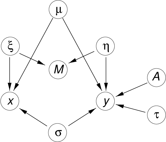
Note that not only and but also does not appear in this expression, principally from our choice of parameterisation, and that only the ratio is identifiable. The directed acyclic graph representing this joint probability model, including the variables (, and ) that we have integrated out, is displayed in Figure 1.
3 Prior distributions and computational implementation
We will henceforth treat and as fixed, and consider inference for the remaining unknowns , , and sometimes , given the data and . Markov chain Monte Carlo methods must be used for the computation; several introductions and overviews of MCMC are available, for example, the primer in Green (2001). In Section 3.6, we discuss the relevance and applicability of an EM algorithm for making inference with an approximation of our model.
We suppose that prior information about , and will be at best weak, and so we concentrate on generic prior formulations that facilitate the posterior analysis. Prior assumptions are therefore discussed in parallel with MCMC implementation. Note that our formulation has some affinity with mixture models, the matching matrix playing a similar role to the allocation variables often used in computing with mixtures; see, for example, Richardson and Green (1997). As in that paper, the fully Bayesian analysis here aims at simultaneous joint inference about both the discrete and continuously varying unknowns, in contrast to frequentist approaches.
Our model has another similarity with a mixture formulation, in that as varies, the number of hidden points needed to generate all the observed data also varies, and thus there seems to be a ‘variable-dimension’ aspect to the model. However, here our approach of integrating out the hidden point locations eliminates the variable-dimension parameter, so that reversible jump MCMC is not needed.
3.1 Priors and MCMC updating for a rotation matrix
We are interested in alignment and matching problems in which either is given, and treated as fixed, or in which it is one of the objects of inference. In the latter case, we consider in this paper only the case of rotation matrices in two and three dimensions. We therefore focus on the full conditional distribution for , which from (6) is
Viewing this as a density for , we are still free to choose the dominating measure for , which is arbitrary: this full conditional density is then with respect to the same measure.
Let us restrict attention to rotations: orthogonal matrices , (those with = ) with positive determinant, so that . Expanding the expression above, we then find
Note a remarkable opportunity for (conditional) conjugacy – if has the form for some matrix , then the posterior has the same form with replaced by
This form of is known as the matrix Fisher distribution (Downs, 1972; Mardia and Jupp, 2000, p. 289). To the best of our knowledge, this unique role of the matrix Fisher distribution (or in the two-dimensional case, the von Mises distribution) as the prior distribution for a rotation conjugate to spherical Gaussian error distributions has not previously been noted. (Although Mardia and El-Atoum (1976) have identified the von Mises–Fisher distribution as the conjugate prior for the mean direction). This may have relevance in models for other situations, including the simpler case where there is no uncertainty in the matching. The conjugacy is presumably related to the interpretation of the matrix Fisher distribution as a conditional multivariate Gaussian (see Mardia and Jupp, 2000, p.289).
Two-dimensional case
Now consider the two-dimensional case, . An arbitrary rotation matrix can be written
and the natural dominating measure for is Lebesgue on . Then a uniformly distributed choice of corresponds to . More generally, the von Mises distribution for
can indeed be expressed as , where a (non-unique) choice for is
Thus the full conditional distribution for is of the same von Mises form, with updated to , and to , where is the matrix .
It is therefore trivial to implement a Gibbs sampler move to allow inference about , assuming a von Mises prior distribution on the rotation angle (including the uniform case, ). We can use the Best/Fisher algorithm, an efficient rejection method (see Mardia and Jupp, 2000, p.43), to sample from the full conditional for .
Three-dimensional case
In the three-dimensional case, we can represent as the product of elementary rotations
| (7) |
as in Raffenetti and Ruedenberg (1970), and Khatri and Mardia (1977). Here, for , is the matrix with , , for and other entries 0. We can then update each of the generalised Euler angles in turn, conditioning on the other two angles and the other variables () entering the expression for .
The joint full conditional density of the Euler angles is
for and . The cosine term arises since the natural dominating measure, corresponding to uniform distribution of rotation, has volume element in these coordinates.
Substituting the representation (7), and simplifying, we find that the trace can be written variously as where
and the can be ignored, combined into the normalising constants. Thus the full conditionals for and are von Mises distributions, and so these two variables can be updated by Gibbs sampling. That of is proportional to
and we use a random walk Metropolis update for this variable, with a perturbation uniformly distributed on . The latter distribution has been studied in Mardia and Gadsden (1977) but with no discussion on how to simulate from it.
3.2 Priors and updating for other parameters
We make the standard normal/inverse gamma assumptions:
Under the assumptions of (6), there is conjugacy for and , and we have explicit full conditionals:
and so it is trivial to implement Gibbs sampler updates for these parameters.
3.3 Updating
The matching matrix is updated in detailed balance using Metropolis-Hastings moves that only propose changes to a few entries: the number of matches can only increase or decrease by 1 at a time, or stay the same. The possible changes are
- (a)
adding a match: changing one entry from 0 to 1
- (b)
deleting a match: changing one entry from 1 to 0
- (c)
switching a match: simultaneously changing one entry from 0 to 1, and another in the same row or column from 1 to 0.
The proposal proceeds as follows: first a uniform random choice is made from all the data points . Suppose without loss of generality, by the symmetry of the set-up, that an is chosen, say . There are two possibilities: either is currently matched ( such that ) or not (there is no such ).
If is matched to , with probability we propose deleting the match, and with probability we propose switching it from to , where is drawn uniformly at random from the currently unmatched points. On the other hand, if is not currently matched, we propose adding a match between and a , where again is drawn uniformly at random from the currently unmatched points.
The acceptance probabilities for these three possibilities are easily derived from the expression (6) for the joint distribution, since in each case the proposed new matching matrix is only slightly perturbed from , so that the ratio has only a few factors. Taking into account also the proposal probabilities, whose ratio is , where is the number of unmatched points in , we find that the acceptance probability for adding a match is
| (8) |
Similarly, the acceptance probability for switching the match of from to is
| (9) |
and for deleting the match it is
where . Along with just one of each of the other updates, we typically make several moves updating per sweep, since the changes effected are so modest.
3.4 Loss functions
The output from the MCMC sampler derived above, once equilibrated, is a sample from the posterior distribution determined by (6). As always with sample-based computation, this provides an extremely flexible basis for reporting aspects of the full joint posterior that are of interest.
The matching matrix will often be of particular inferential interest, and for some purposes a point estimate is desirable; in this section we discuss how to obtain a Bayesian point estimate of the matching matrix .
The most easily understood estimator of would be its posterior mode, the maximum a posteriori (MAP) estimator. However, there are difficulties here. First, the notion is itself ambiguous – the unknown ‘parameter’ in our model consists of the matching matrix , and some real parameters. ‘MAP’ might refer to the component of the overall maximum, or the mode of the marginal posterior for alone. Secondly, the posterior is multi-modal, and different modes may have different ‘widths’, appropriately measured. So there is no intrinsic attraction to the MAP estimate. We should return to basic principles.
By standard theory, this requires specification of a loss function, , giving the cost incurred in declaring the matching matrix to be when it is in fact . The optimal estimate given data is the matching matrix that minimises the posterior expected loss
the expectation over being taken with respect to the posterior determined by (6). In this language, the MAP estimator is optimal for the ‘zero–one’ loss function under which a fixed total cost is paid if there is a single error in any value ; this is logically unappealing, and a further argument against using MAP.
We consider instead loss functions that penalise different kinds of error and do so cumulatively. The simplest of these are additive over pairs . Suppose that the loss when and , for is ; for example, is the loss associated with declaring a match between and when there is really none, that is, a ‘false positive’. Then it is readily shown that
where
and is the posterior probability that is a match, which is estimated from an MCMC run by the empirical frequency of this match. Thus, provided that and , as is natural, the optimal estimate is that maximising the sum of marginal posterior probabilities of the declared matches , penalised by a multiple times the number of matches. The optimal match therefore depends on the four loss function parameters only through the cost ratio . If false positive and false negative matches are equally undesirable, one can simply choose .
Computation of the optimal match would be trivial but for the constraint that there can be at most one positive entry in each row and column of the array. For modest-sized problems, the optimal match can be found by informal heuristic methods. These may not even be necessary, especially if is not too small. In particular, it is immediate that if the set of all pairs for which includes no duplicated or values, the optimal consists of precisely these pairs.
We could also consider loss functions that penalise mismatches differently from the sum of the losses of the individual errors. For example, declaring to be a match when it should be might deserve a relative loss greater or lesser than , depending on context. Such loss functions could be handled in a broadly similar way, but this is left for future work.
3.5 Using partial labelling information
When the points in each configuration are ‘coloured’, with the interpretation that like-coloured points are more likely to be matched than unlike-coloured ones, it is appropriate to use a modified likelihood that allows us to exploit such information. Let the colours for the and points be and respectively. The hidden point model is augmented to generate the point colours, as follows. Independently for each hidden point, with probability we observe neither nor point, as before. With probabilities and , respectively, we observe only an or point, with colour from an appropriate finite set. With probability
we observe an point coloured and a point coloured . Our original likelihood is equivalent to the case , where colours are independent and so carry no information about matching. If and increase, then matches are more probable, a posteriori, and if , matches between like-coloured points are more likely than those between unlike-coloured ones. The case allows the prohibition of matches between unlike-coloured points, a feature that might be adapted to other contexts such as the matching of shapes with given landmarks.
In implementation of this modified likelihood, the MCMC acceptance ratios in Section 3.3 have to be modified accordingly. For example, if and , then (8) has to be multiplied by and (9) by .
Other, more complicated, colouring distributions where the log probability can be expressed linearly in entries of can be handled similarly.
3.6 Alternative approach using the EM algorithm
The interplay between matching (allocation) and parameter uncertainty has something in common with mixture estimation. This might suggest considering maximisation of the posterior by using the EM algorithm, which could of course in principle be applied either to maximum likelihood estimation based on (5) or to MAP estimation based on (6). For the EM formulation, the ‘missing data’ are the matches.
In an exponential family, the EM algorithm alternates between between finding expectations of missing values given data, at current parameter values, and maximising the log-posterior, with missing values replaced by these expectations.
The ‘expectations of missing values’ are just probabilities of matching. These are only tractable if we were to drop the assumption that a point can only be matched with at most one other point – that is, that , . Making this approximation, the E-step is trivial: the expectation of is where is the factor in the joint model, i.e.
The M-step then requires maximising (for given )
over , , – note that here is a function of all three. Although for some individual parameters this seems to be explicit, in the general case we need numerical optimisation.
In summary, EM allows us to study only certain aspects of an approximate version of our model, and is not trivial numerically – so we do not pursue this approach. Obtaining the complete posterior by MCMC sampling gives much greater freedom in inference.
4 Applications
4.1 Matching protein gels
The objective in this example is to match two electrophoretic gels automatically, given the locations of the centres of 35 proteins on each of the two gels. The data are presented in the supplementary information on the web. The correspondence between pairs of proteins, one protein from each gel, is unknown, so our aim is to match the two gels based on these sets of unlabelled points. We suppose it is known that the transformation between the gels is affine. In this case, experts have already identified 10 points; see Horgan et al (1992). Based on these 10 matches, the linear part of the transformation is estimated a priori to be
| (10) |
(Dryden and Mardia, 1998, pp. 20–21, 292–296).
| rank | |||
|---|---|---|---|
| 1 | 15 | 21 | 1 |
| 2 | 19 | 19 | 1 |
| 3 | 8 | 8 | 1 |
| 4 | 3 | 3 | 1 |
| 5 | 2 | 2 | 1 |
| 6 | 31 | 30 | 0.9989 |
| 7 | 6 | 6 | 0.9987 |
| 8 | 4 | 4 | 0.9966 |
| 9 | 5 | 5 | 0.9946 |
| 10 | 10 | 10 | 0.9927 |
| 11 | 24 | 23 | 0.9855 |
| 12 | 7 | 7 | 0.9824 |
| 13 | 32 | 31 | 0.9776 |
| 14 | 1 | 1 | 0.9763 |
| 15 | 9 | 9 | 0.9677 |
| 16 | 26 | 32 | 0.7910 |
| 17 | 12 | 13 | 0.7552 |
| 18 | 21 | 33 | 0.3998 |
| 19 | 26 | 27 | 0.1931 |
| 20 | 35 | 35 | 0.0025 |

Here, we have only to make inference on the translation and the unknown matching between certain of the proteins. The model (6) will therefore be taken to apply, with and with held fixed at (10). The MCMC sampler described in Section 3 was run for 100 000 sweeps, after a burn-in period of 20 000 sweeps, considered on the basis of an informal visual assessment of time series traces to be adequate for convergence. Prior and hyperprior settings were: , , , and . The sampler parameter was set to 0.5. Such a run took about 2 seconds on a 800MHz PC. Acceptance rates for the moves updating were between 0.6% and 2.1%.
The posterior expectation and variance of were estimated to be (to be compared with obtained by Dryden and Mardia (1998)) and
The posterior mean and variance of are 2.050 and 0.1192.
The 20 most probable matches between and points are listed in Table 1; note that there is no duplication in their indices until the 19th match: also appears in the 16th match (recall that there is a simple rule for identifying the optimal if there are no duplicates among the matches with above the threshold ). We can conclude that for all values of from 1 down to 0.1112, the optimal Bayesian matching is given by an appropriate subset of Table 1, reading down from the top. For example if this cost ratio is 0.8 we take the first 15 rows of the table, while if the ratio is 0.6 or 0.4 we include the 16th and 17th rows as well. The 17 most probable matches are displayed graphically in Figure 2.
It will be noted that all of the expert-identified matches, points 1 to 10 in each set, are declared to be matches with high probability in the Bayesian analysis. We also repeated the analysis with these 10 pairs held fixed. The next 9 most probable matches, together with these 10, are identical to those in the first 19 lines of Table 1, and the posterior probabilities differ by less than 0.037 in all 19 cases.
4.2 Aligning proteins in three dimensions
We now apply the matching method to a problem in three dimensional structural biology, previously considered by Gold et al (2002). The problem consists of finding the matches for two Active sites 1 and 2 corresponding to two Proteins A and B respectively. The corresponding coordinates and of these sites are presented in the supplementary information; these coordinates are the centres of gravity of the amino acids of the two sites. Here and . The biological details of the two proteins are as follows. Protein 1 is the human protein ‘17–beta hydroxysteroid dehydrogenase’ and is involved in the synthesis of oestrogens. This protein binds the ligands (molecules comparatively smaller than proteins) oestradiol and NADP. Protein 2 is the mouse protein ‘carbonyl reductase’ and is involved in metabolism of carbonyl compounds. This protein binds the ligands 2–Propanol and NADP. The common element between these two sets of ligands is NADP. From chemical properties of the sites, the relevant matching should be invariant under rigid transformation.


There is information about the identities of the amino acids in the two configurations: we defer use of this to Section 4.4.
The MCMC sampler described in Section 3 was run for 1 000 000 sweeps, after a burn-in period of 200 000 sweeps, considered on the basis of an informal visual assessment of time series traces to be adequate for convergence. Prior and hyperprior settings were: , , , , and the matrix defining the prior for set to the zero matrix. The sampler parameter was set to 0.5, and we made updates to 10 times in each sweep. Such a run took about 71 seconds on a 800MHz PC. Acceptance rates for the moves updating were between 0.41% and 5.6%.
The posterior expectation and variance of were estimated to be and
The posterior mean and variance of are 1.051 and 0.00996. In representing the centre of the posterior distribution for the rotation matrix , we we need to use a definition of mean appropriate to the geometry. We form the mean elementwise from a thinned sample of 2000 values of from the post-burn-in MCMC run. This mean matrix is of course not a rotation matrix, but post-multiplication by the positive definite symmetric square root of yields a rotation matrix that is known as its polar part (see Mardia and Jupp, p. 286, 290). This is an appropriate measure of location of the posterior, and takes the value
| (11) |
in this case.
The 40 most probable matches between and points are listed in supplementary information; there is no duplication in their indices until the 39th match: also appears in the 38th match. We can conclude that for all values of greater than 0.2895 (the marginal posterior probability associated with the 39th match), the optimal Bayesian matching is given by an appropriate leading subset of the matches. For example if this cost ratio is 0.5 we take the first 36 matches; these are displayed graphically in Figure 3; in this 3-dimensional example, the axes signify the first two principle coordinates of the combined cloud of data.
As would be anticipated, simultaneous inference for the rotation and the matching matrix (as well as and ) is a considerably greater challenge for MCMC than is the problem of the previous section, where the rotation matrix is held fixed. It is clear that there is a possibility of severe multi-modality in the posterior, with the conditional posterior for and given depending strongly on . This challenge is quantified empirically by a heavy-tailed distribution of times to convergence, and by ‘meta-stability’ in the time series plots of various monitoring statistics against simulation time. We found the log-posterior to be a useful summary statistic for quality of fit, and pilot runs provided experience to choose a threshold value, exceedance of which we hypothesised diagnosed convergence to the main mode of the posterior.
To investigate multimodality and convergence time, we conducted a study in which the MCMC run described was repeated – with the same parameters – from 100 different initial configurations, obtained by independent random rotations as initial settings for . After short runs of 50 000 sweeps, we tested whether the threshold log-posterior value had been exceeded, and if not the run was abandoned. 83 out of the 100 runs passed this test, and these were allowed to run on for a further 450 000 sweeps. Every one of these 83 long runs provided exactly the same set of 36 most probable matches, and we therefore felt justified to conclude that they had not been trapped in a subsidiary mode of the posterior, and that it was safe to draw inference from the results. This conclusion is specific to the data set and parameter settings used, and it would be straightforward to contrive artificial data where multiple modes were more equal in probability content. In such cases more sophisticated MCMC samplers would be needed.
4.3 Prior settings and sensitivity
Our analysis depends of course on the settings of the hyperparameters (see Section 2.2), (Section 3.1), and , , , (Section 3.2). These allow the provision of real prior information from the experimental context, if it is available.
For a default analysis in the absence of such information, we would set to the zero matrix (a uniform prior on ), to be the zero vector, and of the order of twice the distance between the centres of gravity of the two configurations. We fix , giving an exponential prior distribution for . Here we briefly discuss settings of, and sensitivity to, the remaining two parameters, the scalars and .
Sensitivity to is pronounced, as might be anticipated. This parameter ratio has a very direct role in determining whether an pair are noisy observations of the same hidden point or not, after transformation, since it controls the density of hidden points. In practice, we should not expect to be able to draw inference about matching without real prior knowledge about this ratio or an equivalent measure of the prior tendency of points to be matched.
The prior for the number of matches is parameterised by : see (3). This distribution is non-standard, but very well-behaved. It is clear from inspection that setting equal to yields a mode of that is within 1 of , and numerical calculation in the context of the example in Section 4.2, verifies that for all possible ‘prior guesses’ for , the prior expectation and median are also both equal to to the nearest integer. Thus prior information about is directly informative about the parameter ratio . As long as is known, or at least a representative value provided, and the analyst is able to make a prior guess at the number of matches, this suggests a reasonable way to specify . The posterior distribution for tracks the prior rather closely, confirming that the raw data carry little information about the number of matches.
The hyperparameter is an inverse scale parameter for the precision of the noise terms ; thus as increases, we expect that increases too. The runs we have presented used ; reducing this by a factor of 2 makes minimal difference to the posterior inference for either or . However, increasing by a factor of 2 leads to a 3-fold increase in and a sharp reduction in the number of matches – the posterior expectation of goes down from around 34 to 26. The latter observation is perhaps counter-intuitive, until one realises that when is larger, it becomes relatively less likely that points that are nearly coincident (after transformation) are in fact matched.
Finally, it would be desirable to assess the sensitivity to the Poisson assumption for the hidden point model, but this would be extremely onerous to do directly, since alternatives would require a substantially modified formulation and implementation. There is scientific reason to doubt the Poisson assumption; for example, the minimum spacing between the centres of gravity of the amino acids in proteins is approximately 3.8 Angstroms. However, experiments reported in Mardia, Nyirongo and Westhead (2005) do at least suggest strongly that the ability of our method to detect matches is little affected by real hard-core effects.
4.4 Using information about types of amino acid
The protein alignment data includes identifiers of the type of amino acid at each point (see supplementary information). There are 20 different types, which can be categorised into 4 groups: hydrophobic, charged, polar and glycine; we use the group identifiers as colours in defining a modified likelihood as in Section 3.5. The parameter values taken were and , providing a strong preference for like-coloured matching (). The analysis was repeated with this modified model, leaving all other details unchanged.
The 40 most marginally probable matches are listed in supplementary information, along with displayes of the optimal alignment. The 36 most probable matches, which together form the optimal matching whtn , are identical to those found in the previous section; however, there are modest variations in the posterior probabilities attached to individual matches.
The posterior expectation and variance of were now estimated to be (slightly shifted from that obtained in the analysis of the previous section) and
The posterior mean and variance of are 1.3122 and 0.1984. The increased estimate of is perhaps anticipated. The centre of the posterior distribution of is in this case:
| (12) |

In the approach to the analysis of these data taken by Gold et al (2002), the matching between the configurations was performed in two stages, and is not driven by an explicit probability model. First, inter-point distances were calculated within each configuration. These distances are invariant under the rigid body motions considered here. A maximal set of pairs of indices , with no ties among the s or s, is found such that is less than some threshold, for all . This is done using graph theoretical algorithms of Bron and Kerbosch (1973) and Carraghan and Pardos (1990), applied to a product graph whose vertices are labelled with pairs. This first stage of the matching alogrithm was formulated by Kuhl et al (1984).
In the second stage, the matches are scored using the amino acid information, assigning a score of 1 for identity of the amino acids, and 0.5 when the amino acids are different but fall in the same group. The initial list of matches from stage one is then permuted so as to maximise the total score.
Once the matches are found the rigid body transformation is estimated by Procrustes analysis; for example, see Dryden and Mardia (1998, pp 176-178).
It is interesting to compare the rotation matrix resulting from this method, namely
with that obtained by our method. The trace of the orthogonal matrix taking to is approximately , so the two differ by a rotation of only 0.07 radians. Figure 5 provides a comparison between the matchings achieved by the two approaches. Of the 27 matches identified by Gold et al, 14 are among the most probable 20 that we find, and all 27 are among the first 35.
A referee has raised with us the role of sequence ordering along the protein in inference about alignment and matching. The example in this section concerns ligand binding site matching, in which biologically relevant matches do not necessarily preserve sequential ordering, in contrast to the more familiar situation of aligning protein backbones; see for example Eidhammer et al (2004, pp. 333–334). Examples are trypsin-subtilisin with similar active sites and unrelated folds, and many adenine binding sites in different folds. Somewhat remarkably, although sequence ordering is not used in our analysis, the resulting matches do perfectly respect this ordering. This is visualised in Figure 5, which also reveals that some but not all of the matches revealed by our analysis additional to those of Gold et al (2002) extend already matched segments. In this particular data set, the sites must come from very closely related folds and would probably also be alignable by sequence-preserving methods aligning full structures. Intriguingly, in this example at least, knowledge of the sequence ordering would provide no additional information beyond that extracted from the point coordinates and amino-acid groups by our approach.
5 Discussion
The main conclusion of this paper is that a probability model based approach is successful in allowing simultaneous inference about partial matching between two point configurations, and a geometrical transformation between the coordinate systems in which the configurations are measured. This seems an advance over previous more ad-hoc methods.
We have only used the translation and rigid motion groups in illustrating our methodology. However, the formulation allows inference about various other group transformations such as affine transformation, and so on. The fairly straightforward MCMC implementation presented here has proved adequate for the models and data sets considered, although allowing rotations did increase the needed run lengths considerably. We anticipate that, at least for models allowing rotations, dealing with larger data sets will be much more challenging, since small rotational perturbations generate large displacements at sites far from the axis of rotation; moves that simultaneously perturb allocations and geometrical and error distribution parameters will be necessary for good performance. We also anticipate more severe difficulties from multi-modality that were exposed in Section 4.2.
An important task left for future work is a formulation that allows smooth nonparametric transformations between coordinate systems, setting warping into a model-based framework; this would be important in dealing more comprehensively with gel matching problems.
We have only used pairwise comparisons but there is scope for taking multiple combinations such as triads. The transformations considered above are parametric but some non-parametric alternatives such as non-linear deformations may be useful in some cases, e.g. to deal with dynamic aspects of the atoms in a protein. We have considered only two configurations but a natural extension would be to take three or more point configurations simultaneously, and make joint inference about patterns of matching between the configurations and the various geometrical transformations involved. More straightforward extensions would be to allow for non-Gaussian noise, other types of prior and so on.
Kent et al (2004) have treated the unlabelled case by using a different model. While matching two configurations, one of them is taken as the population and the second as a random sample from this population after an unknown transformation. This approach is different from the symmetrical model for the two configurations proposed here. Further the emphasis in Kent et al (2004) is on maximum likelihood inference using the EM-algorithm.
Recent independent work by Dryden, Hirst and Melville (2005), addresses a similar problem of matching unlabelled point sets. Their approach has some substantial differences, for example there is assymmetry in comparing two configurations, one being treated as a perturbation of the other. The geometrical transformation parameters are given uniform priors and maximised out, using standard ideas from shape analysis, rather than integrated out as in our fully Bayesian approach. Neither the loss function basis for estimating matches, nor the treatment of partial labelling, appear.
There is other statistical work on alignment and matching in proteins by Wu et al (1998) and Schmidler (2004), which in contrast does use sequence information. Further work is needed to clarify the relationships between all these methods and their comparative performance.
Finally, in the context of using methods such as ours in database search, often the reason for assessing protein alignment, there are issues related to multiple comparisons. These are not discussed here, but the answers will depend on the size of the database as well as the number of points in the query site.
Acknowledgements
We are grateful to Nicola Gold and Dave Westhead for their many helpful discussions, and in particular for the data in Example 2, and to Vysaul Nyirongo and Charles Taylor for various helpful comments.
References
-
Abramowitz, M. and Stegun, I. A. (1970). Handbook of Mathematical Functions. Dover, New York.
-
Bron, C. and Kerbosch, J. (1973). Algorithm 457; finding all cliques of an undirected graph. Communication of the ACM, 16, 575–577.
-
Carraghan, R. and Pardalos, P. M. (1990). Exact algorithm for the minimal clique problem. Operations Research Letters, 9, 375.
-
Chui, H. and Rangarajan, A. (2000). A new algorithm for non-rigid point matching. IEEE Conference on Computer Vision and Pattern Recognition. 2, 44–51.
-
Cross, A. D. J. and Hancock, E. R. (1998). Graph matching with dual-step EM algorithm. IEEE transactions on pattern analysis and machine intelligence. 20, 1236–1253.
-
Downs, T. D. (1972). Orientation statistics. Biometrika, 59, 665–676.
-
Dryden, I. L., Hirst, J. D. and Melville, J. L. (2005). Statistical analysis of unlabelled point sets: comparing molecules in chemoinformatics. Under revision for Biometrics.
-
Dryden, I. L. and Mardia, K. V. (1998). Statistical shape analysis. Wiley, Chichester.
-
Eidhammer, T., Jonassen, T. and Taylor, W. R. (2004). Protein Bioinformatics. Wiley, Chichester.
-
Gold, N. D., Pickering, S. J., and Westhead, D. R. (2002). Protein functional site matching using graph theory techniques. In Proceedings of the International Conference on Bioinformatics, Bangkok, Thailand, page 79.
-
Green, P. J. (2001). A Primer on Markov chain Monte Carlo, pp. 1–62 of Complex Stochastic Systems, Barndorff-Nielsen, O. E., Cox, D. R. and Klüppelberg, C. (eds.), Chapman and Hall, London.
-
Horgan, G. W., Creasey, A. and Fenton, B. (1992). Superimposing two dimensional gels to study genetic variation in malaria parasites. Electrophoresis, 13,871–875.
-
Kent, J. T., Mardia, K. V. and Taylor, C. C. (2004). Matching problems for unlabelled configurations. In Bioinformatics, Images and Wavelets, edited by Aykroyd, R.G., Barber, S. and Mardia, K.V. Proceedings of LASR 2004, Leeds University Press, Leeds.
-
Khatri, C. G. and Mardia, K. V. (1977). The von Mises–Fisher distribution in orientation statistics. Journal of the Royal Statistical Society, B, 39, 95–106.
-
Kuhl, F. S., Crippen, G. M. and Friesen, D. K. (1984). A combinatorial algorithm for calculating ligand binding. Journal of Computational Chemistry, 5, 24–34.
-
Mardia, K. V. and El-Atoum, S. A. M. (1976). Bayesian inference for the von Mises–Fisher distribution. Biometrika, 63, 203–205.
-
Mardia, K. V. and Gadsden, R. J. (1977). A circle of best fit for spherical data and areas of vulcanism. Applied Statistics, 26, 238–245.
-
Mardia, K. V. and Jupp, P. E. (2000). Directional Statistics, Wiley, Chichester.
-
Mardia K. V., Taylor, C. C, and Westhead, D. R. (2003). Structural bioinformatics revisited. In LASR2003, pp11–18. Leeds University Press.
-
Mardia, K. V., Nyirongo, V., and Westhead, D.R. (2005). EM algorithm, Bayesian and distance approaches to matching active sites Mathematical and Statistical Annual Meeting in Bioinformatics, Rothamsted, March 2005, Abstracts pp13-14.
-
Pedersen, L. (2002). Analysis of two-dimensional electrophoresis gel images. Ph.D thesis, IMM Technical University of Denmark.
-
Raffenetti, R. C. and Ruedenberg, K. (1970). Parameterization of an orthogonal matrix in terms of generalized Eulerian angles. International Journal of Quantum Chemistry, IIIS, 625–634.
-
Richardson, S. and Green, P. J. (1997). On Bayesian analysis of mixtures with an unknown number of components (with discussion). Journal of the Royal Statistical Society, B, 59, 731–792.
-
Schmidler, S. C. (2004). Bayesian shape matching and structural alignment. Presentation at the 6th World Congress of the Bernoulli Society, Barcelona, July 2004.
-
Wu, T. D., Schmidler, S. C., Hastie, T. and Brutlag, G. (1998). Regression analysis of multiple protein structures. Journal of Computational Biology, 5, pp 585–595.