There are many problems in science which are too complex for numerical solution as they stand. Examples include turbulence and other problems where multiple scales must be taken into account. Such problems must be reduced to more amenable forms before one computes. In the present paper we would like to summarize some reduction methods that have been developed in recent years, together with an account of what was learned in the process. It is obvious that the problem has not been fully solved, but we think that the examples and the conclusions reached so far are useful.

In general terms, a reduction to a more amenable form is a renormalization group transformation, as in physics — a transformation of a problem into a more tractable form while keeping quantities of interest invariant. A renormalization group transformation involves an incomplete similarity transformation (see below for definitions), and thus a reduction method is a search for hidden similarities. This a general feature of reduction methods, and it will be illustrated in the examples. A successful problem reduction produces a new problem which must in some asymptotic sense be similar to the original problem. For general backgound on renormalization, see e.g.[6, 21, 39].

In problems with strong time dependence, reduction methods resemble methods for the analysis of thermodynamic systems not in equilibrium; indeed, those aspects of the problem that are ignored in a reduced description conspire to destroy order and increase entropy. Problem reduction for time-dependent problems is basically renormalization group theory for non-equilibrium statistical mechanics. For background on such theory, see e.g. [3, 23, 9].

The content of the paper is as follows: In section 2 we consider Hamiltonian systems and their conditional expectations. In section 3 we narrow the discussion to statistically stationary Hamiltonian systems and recover Kadanoff real-space renormalization groups and an interesting block Monte-Carlo method. In section 4 we display an example that exhibits and also extends the main features of this analysis in simple form.

In section 5 we explain the Mori-Zwanzig formalism for the reduction of statistically time-dependent problems. The analysis shows that averaging the equations is in general not enough; one must take into account noise and a temporal memory. The Mori-Zwazig formalism is rather dense, and in the sections that follow we present various special cases in which it can be simplified, in particular when the memory is very short or very long.

For the sake of readability, we remind the reader of the rudiments of similarity theory [3]. Suppose a variable $a$ is a function of variables $a_{1},a_{2},\ldots,a_{m}$, $b_{1},b_{2},\ldots,b_{k}$, where $a_{1},\ldots,a_{m}$ have independent units, for example units of length and mass, while the units of $b_{1},\ldots,b_{k}$, can be formed from the units of $a_{1},a_{2},\ldots,a_{m}$. Then there exist dimensionless variables $\Pi=\frac{a}{a_{1}^{\alpha_{1}}\cdots a_{m}^{\alpha_{m}}}$, $\Pi_{i}=\frac{b_{i}}{a_{1}^{\alpha_{i1}}\cdots a_{m}^{\alpha_{im}}}$, $i=1,\ldots,k$, where the $\alpha_{i},\alpha_{ij}$ are simple fractions, such that $\Pi$ is a function of the $\Pi_{i}$:

$$\Pi=\Phi(\Pi_{1},\ldots,\Pi_{k}).$$

(1)

This is just a consequence of the requirement that a physical relationship be independent of the size of the units of measurement. At this stage nothing can be said about the function $\Phi$. Now suppose the variables $\Pi_{i}$ are small or large, and assume that the function $\Phi$ has a non-zero finite limit as its arguments tend to zero or to infinity; then $\Pi\sim$ constant, and one finds a power monomial relation between $a$ and the $a_{i}$. This is a complete similarity relation. If the function $\Phi$ does not have the assumed limit, it may happen that for $\Pi_{1}$ small or large, $\Phi(\Pi_{1})=\Pi_{1}^{\alpha}\Phi_{1}(\Pi_{1})+\ldots$, where the dots denote lower order terms, $\alpha$ is a constant, the other arguments of $\Phi$ have been omitted and $\Phi_{1}$ has a finite non-zero limit. One can then obtain a scaling (power monomial) expression for $a$ in terms of the $a_{i}$ and $b_{i}$, with undetermined powers which must be found by means other than dimensional analysis. The resulting power relation is an incomplete similarity relation. Of course one may well have functions $\Phi$ with neither kind of similarity.

Incomplete similarity expresses what is invariant under a renormalization group; all renormalization group transformations involve incomplete similarity, see the books already cited as well as [5] written before the notion of incomplete similarity was formalized. The exponent $\alpha$ is called an anomalous exponent.

The paper [22] is a survey of reduction methods organized along different lines and can be profitably read in tandem with the present paper.

We begin by examining what happens when one tries to reduce the complexity of a Hamiltonian system by averaging (see also [17, 18, 38]). Consider a system of nonlinear ordinary differential equations,

	$\displaystyle\frac{d}{dt}\varphi(t)$	$\displaystyle=$	$\displaystyle R(\varphi(t)),$
	$\displaystyle\varphi(0)$	$\displaystyle=$	$\displaystyle x,$		(2)

where $\varphi$ and $x$ are $n$-dimensional vectors with components $\varphi_{i}$ and $x_{i}$, and $R$ is a vector-valued function with components $R_{i}$; $t$ is time. To each initial value $x$ in (2) corresponds a trajectory $\varphi(t)=\varphi(x,t)$.

Suppose that we only want to find $m$ of the $n$ components of the solution vector $\varphi(t)$ without finding the $n-m$ others. One has to assume something about the variables that are not evaluated, and we assume that at time t=0 we have a a joint probability density $F(x)$ for all the variables. The variables we keep will have definite initial values $x_{1},x_{2},\dots,x_{m}$, and the rest of variables will then have a conditional probability density $f_{m}=f(x_{1},\dots,x_{m},x_{m+1},\dots)/Z_{m}$, where $Z_{m}=\int_{-\infty}^{+\infty}f(x_{1},\dots,x_{m},x_{m+1},\dots)dx_{m+1}dx_{m+2}\cdots$ is a normalization constant. Without some assumption about the missing variables the problem is meaningless; this particular assumption is reasonable because in practice $f$ can often be estimated from previous experience or from general considerations of statistical mechanics. The question is how to use this prior knowledge in the evaluation of $\varphi(t)$.

Partition the vector $x$ so that ${\hat{x}}=(x_{1},x_{2},\dots,x_{m})$, $\tilde{x}=(x_{m+1},\dots,x_{n})$ and $x=(\hat{x},\tilde{x})$, and similarly $\varphi=(\hat{\varphi},\tilde{\varphi}),R=(\hat{R},\tilde{R})$. In general the first $m$ components of $R$ depend on all the components of ${\varphi}$, ${\hat{R}}={\hat{R}}(\varphi)={\hat{R}}(\hat{\varphi},\tilde{\varphi})$; if they do not we have a system of $m$ equations in $m$ variables and nothing further needs to be done. We want to calculate only the variables $\hat{\varphi}$; then $(d/dt)\hat{\varphi}(t)=\hat{R}(\varphi(t))$ where the right hand side depends on the variables $\tilde{\varphi}$ which are unknown at time $t$. We shall call the variables $\hat{\varphi}$ the “resolved variables” and the remaining variables $\tilde{\varphi}$ the “unresolved variables”.

Consider in particular a Hamiltonian system as in [17],[18]. There exists then a Hamiltonian function $H=H(\varphi)$ such that for $i$ odd $R_{i}$, the $i$-th component of the vector $R$ in (2) satisfies $R_{i}=\partial H\bigl/{\partial\varphi_{i+1}}$ while for $i$ even one has $R_{i}=-{\partial H}\bigl/{\partial\varphi_{i-1}}$, with $n$, the size of the system, even. Assume furthermore that $f$, the initial probability density, is $f(\varphi)=Z^{-1}\exp(-H/T)$ where $T$ is a parameter, known in physics as the “temperature”, which will be set equal to one in much, but not all, of the discussion below. In physics this density appears naturally and is known as the “canonical” density; the normalizing constant $Z=Z(T)$ is the “partition function”. This density $f$ is invariant, i.e. sampling it and evolving the system in time commute.

A numerical analyst who wants to approximate the solution of an equation usually starts by approximating the equation. If one solves for the resolved variables one has values for the variables $\hat{\varphi}$ available at each instant $t$ and the best approximation should be a function of these variables; it is natural to seek a best approximation in the mean square sense with respect to the invariant density $f$ at each time; the best approximation in this sense is the conditional expectation $E[R(\varphi)|\hat{\varphi}]=\int e^{-H}d\tilde{\varphi}\bigl/\int e^{-H}d\tilde{\varphi}$ (note that we set $T=1$). This conditional expectation is the orthogonal projection of $R$ onto the space of functions of $\hat{\varphi}$ with respect to the inner product $(u,v)=E[uv]=\int u(\varphi)v(\varphi)f(\varphi)d\varphi$, where $d\varphi$ denotes integration over all the components of $\varphi$. We then try to approximate the system (2) by:

	$\displaystyle\frac{d}{dt}\hat{\varphi}(t)$	$\displaystyle=$	$\displaystyle E[R(\varphi(t))|\hat{\varphi}(t)],$
	$\displaystyle\hat{\varphi}(0)$	$\displaystyle=$	$\displaystyle\hat{x}.$		(3)

We have shown in [15, 17, 13] that: (i) The new system (3) is also Hamiltonian:

$$E\left[\frac{\partial H}{\partial\varphi_{i}}|\hat{\varphi}(t)\right]=\int\frac{\partial H}{\partial\varphi_{i}}\exp(-H)d\tilde{\varphi}\bigl/\int\exp(-H)d\tilde{\varphi}=\frac{\partial\hat{H}}{\partial\varphi_{i}},$$

(4)

where $i\leq m=$ the dimension of $\hat{\varphi}$, and

$$\hat{H}=-log\int\exp(-H)d\tilde{\varphi}$$

(5)

is the new Hamiltonian.

(ii) The new canonical density $\hat{f}=Z^{-1}\exp(-\hat{H})$ is invariant in the evolution of the new, reduced, system.

(iii) When the data are sampled from the canonical distribution, the distribution of $\hat{\varphi}$ in the new system is its marginal distribution in the old system; equivalently, the partition function $Z$ is the same for the old system and for the new system.

Now the question is, what does the solution $\hat{\varphi}(t)$ of (3) represent ? It does not approximate the first $m$ components of the solution $\varphi(t)$ of (2)- the components of $\hat{\varphi}$ and the components of $\varphi$ live in spaces of different dimension and in general the components of the latter in those higher $n-m$ dimensions are not small. One could hope that what the solution of (3) approximates is the vector $E[\hat{\varphi}(t)|{\hat{x}}]$, the best estimate of the first components of the solution at time $t$ given the partial initial information ${\hat{x}}$. This is the case for linear systems (where averaging and time integration commute), and is approximately the case for limited time in some other special situations- nearly linear systems, some systems where the “unresolved variables” are fast. However, in general this is not the case. We shall see below that a reduced description of the solution of nonlinear systems in time requires in general “noise” and a “memory”.

The lack of convergence can be understood by the following physics argument. In physics a system in which the values of all the variables are drawn from a canonical distribution is a system in thermal equilibrium. The assignment of definite values $\hat{x}$ to the variables $\hat{\varphi}$ at time $t=0$ amounts to taking the system out of equilibrium at $t=0$; if the system is ergodic it will then decay to equilibrium in time, so that all the variables become randomized and acquire the joint density $f$. Thus the predictive value of the partial initial data $\hat{x}$ decreases in time; all averages of the $\hat{\varphi}$ approach equilibrium averages. However, the reduced system (3) is Hamiltonian, and the solutions it produces oscillate forever.

In Figure 1 we consider the Hald Hamiltonian system ([15]) with

$$H=\frac{1}{2}\left(\varphi_{1}^{2}+\varphi_{2}^{2}+\varphi_{3}^{2}+\varphi_{4}^{2}+\varphi_{1}^{2}\varphi_{3}^{2}\right)$$

(6)

(physically, two linear oscillators with a nonlinear coupling). We assume that $\varphi_{1}(0),\varphi_{2}(0)$ are given and sample the two other initial data from the canonical distribution with $T=1$.

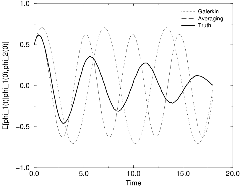
In Figure 1 are displayed (1) The result for $\varphi_{1}$ of a “Galerkin” calculation in which the unresolved variables are set to zero (this is what is implicitly done in many unresolved computations); (2) the result of the averaging procedure just described, and (3) the true $E[\varphi_{1}(t)|{\hat{x}}]$, calculated by repeatedly sampling the initial data, solving the full system, and averaging. As one can see, averaging is initially better than the null “Galerkin” method, but in the long run the truth decays but the solution of the averaged system oscillates for ever. For more detail, see [15].

The procedure we have just described resembles sufficiently the averaging methods used in some areas of engineering, for example the large-eddy simulation methods in turbulence (see e.g. [32]) and in some multiscale problems (see e.g. [44]), to cast a very serious doubt on the broad validity of the latter. For a description of special cases, with small fluctuations and particular structures, where this procedure is legitimate, see [22].

There is however a case where the construction of the preceding section can be very useful– when $m=0$, i.e., when one tries to predict the future with no initial information. Equations (2) then sample the canonical distribution and the reduced system samples a subset of variables without sampling the others, and, as we have seen, keep the statistics of the resolved variables unchanged (see [38] for an application to molecular dynamics).

To see what is happening, suppose the variables $\varphi_{i}$ are associated with nodes on a regular lattice, for example, they may represent spins in a solid, or originate in the spatial discretization of a partial differential equation.

Divide the lattice into blocks of some fixed shape (for example, divide a regular one-dimensional lattice into groups of two contiguous nodes). We had not yet specified how the variables are to be divided into resolved and unresolved. Now decide to “resolve” one variable per block, and leave the others in the same block unresolved. The transformation between the old variables and the smaller set of resolved variables is a Kadanoff renormalization group transformation [29]; the Hamiltonian $\hat{H}$ defined above in equation (5) is the renormalized Hamiltonian. We will now explain what this means.

Suppose the system described by the Hamiltonian is translation invariant. The equations of motion for any at any one point, say at the location labeled by $1$, have the same form as the equations of motion at any any other point. The relation between the right hand side of the reduced system and the right hand side of the old system can be rewritten as:

$$\frac{\partial\hat{H}}{\partial\varphi_{1}}=E[\frac{\partial H}{\partial\varphi_{1}}|\hat{\varphi}],$$

(7)

where the expected value is with respect to the invariant density as before. This relation is the starting point for the actual evaluation of $\hat{H}$.

Hamiltonians are functions of the variables $\varphi$. They can be expanded in the form:

$$H=\sum_{j}a_{j}\psi_{j},$$

(8)

where the $\psi_{j}$ are “elementary Hamiltonians”. In a translation invariant system, where each equation has the same form as any other, the Hamiltonian is made up of sums over $i$ of terms of the form $h(\varphi_{j}\varphi_{j})$ for various values of $j$, where $h$ is some function; these terms represent “couplings” between variables $j$ apart; one can then choose the elementary Hamiltonians to be polynomials in $x_{i}x_{i+j}$ with a fixed $j$ in each $\psi_{j}$, i.e., one segregates the couplings between variables $j$ apart into separate terms.

In a homogeneous system where there is only one variable per site it is enough to satisfy (7) for one variable, say for $\varphi_{1}$. Define $\psi^{\prime}=\frac{\partial}{\partial\varphi_{1}}\psi$, noting that though $\psi$ is necessarily a function with at least as many arguments as there are components on $\varphi$, $\psi^{\prime}$ can be sparse. Equation (7) reduces to

$$\frac{\partial\hat{H}}{\partial\varphi_{1}}=\sum_{j}a_{j}P\psi^{\prime}_{j}(\varphi)=\sum_{j}\hat{a}_{j}\psi^{\prime}_{j}(\hat{\varphi}),$$

(9)

with the projection $P$ defined as before by $Pg(\varphi)=E[g|\hat{\varphi}]$ for any function $g$ of $\varphi$. Now we’re almost done. One can pick a basis in $\hat{L}_{2}$, the subspace of square integrable functions that depend only on the variables $\hat{\varphi}$, which consists of a subset of the set of functions $\psi^{\prime}$. The right-hand of equation (9) is then a linear combination of $\psi^{\prime}s$; integration with respect to $\varphi_{1}$ requires only the erasure of the primes and yields a series for $\hat{H}$. The elements of $\tilde{\varphi}$ are now gone, and one can relabel the remaining variables $\hat{\varphi}$ so that the terms in the series have exactly the same form as before; the calculation can then be repeated, yielding a sequence of Hamiltonians with ever fewer variables: $H,H^{(1)}=\hat{H}$, $H^{(2)}=\hat{H}^{(1)},\dots$. The corresponding densities $f^{n}=Z^{-1}\exp(-H^{(n)}/T)$ can in principle be sampled by any sampling scheme, for example by Metropolis sampling (but there are caveats, see e.g. [10]).

At this point we have reduced the number of variables by a factor $L$ equal to the number of variables in each block, but this may well seem to be a pyrrhic victory. The Hamiltonians one usually encounters are simple, in the sense that they involve few couplings- finite differences typically link a few neighboring variables, and so do the usual spin Hamiltonians in physics. As one reduces the number of variables, the new Hamiltonians become more complex, with more terms in the series (8); the cost per time step of solving the equations in time or of the cost per move in a Metropolis sampling typically increases fast as well. To see what has been gained one must turn to the physics literature (see e.g. [29].[25]).

Consider the spatial correlation length $\ell$ which measures the range of values of $|j|$ over which the spatial covariances $E[\varphi_{i}\varphi_{i+j}]$ are non negligible, and the correlation time $\tau$ for which the temporal covariances $E[\varphi_{i}(t)\varphi(t+s)]$ are non-negligible. For very large and very small values of the temperature $T$ (the variance parameter in the density $f$) both the correlation time and the correlation length are small; the properties of the system can then be found from calculations with a small number of variables and it is not urgent to reduce the number of variables. There is a range of intermediate values of $T$ for which the correlation length and time for are large and then the reduction is worthwhile. There often is a value $T_{c}$ of $T$, the “critical value”, for which $\ell=\infty$. Values of $T$ around $T_{c}$ are often of great interest.

Now we can see what the reduction can accomplish. If one tries to compute averages with $T$ near $T_{c}$ one finds that the cost of computation is proportional to $\tau$- one has to compute long enough to obtain independent samples of $\varphi$, and a new independent sample will not appear until a time $\sim\tau$ has passed. The reductions above produce a system with smaller $\ell$ and $\tau$ and therefore computation takes less time. Though we started with the declared goal of reducing the number of variables, what has been produced is more interesting: a new system with shorter correlations which is more amenable to computation. It is not the raw number of variables that matters.

The renormalization can be used with a multigrid scheme, in which one runs up and down on different levels of renormalization, on the finer ones to achieve accuracy and the cruder ones to move fast from one macroscopic configuration to another. A comparison with other multigrid sampling schemes (see e.g. [8]) reveals that we have derived a reasonably standard scheme, with however a particularly effective way to store conditional expectations. For details see [10].

An alternative method for obtaining the expansion coefficients for the renormalized Hamiltonians was proposed in [41]. The method is based on the maximization of the likelihood of the renormalized density. The maximization of the likelihood leads to a moment-matching problem. The moments in this case are the expectation values of the ”elementary Hamiltonians” (see above) with respect to the renormalized density. The solution of the moment matching problem yields the expansion of the renormalized Hamiltonian.

The recognition of the links of probability with renormalization is largely due to Jona-Lasinio (see e.g. [27]). The connection of renormalization with incomplete similarity is too well known (see [3, 29, 23]) to require further comment here.

As an illustration of the ideas in the previous section, consider the equation

$$u_{t}+uu_{x}=\epsilon u_{xx}-\beta u_{xxx},$$

(10)

with boundary conditions

$$u(-\infty)=u_{0},\ \ u(+\infty)=0,\ \ u_{x}(-\infty)=0,$$

(11)

where the subscripts denote differentiation, $x$ is the spatial variable, $t$ is time, $\epsilon>0$ is a diffusion coefficient, $\beta>0$ is a dispersion coefficient and $u_{0}>0$ is a given constant. The boundary conditions create a traveling wave solution moving to the right (towards $+\infty$) with velocity $u_{0}/2$ which becomes steady in a moving framework as $t\rightarrow\infty$. In nondimensional form the equation can be written as:

$$u_{t}+uu_{x}=\frac{1}{R}u_{xx}+u_{xxx},$$

(12)

with $u_{x}(-\infty)=0$, $u(+\infty)=0$, $u(-\infty)=1$; $R=\epsilon\sqrt{U}/\alpha$ is a “Reynolds number”. For $R\leq 1$ the traveling wave has a monotonic profile, while for $R>1$ the profile is oscillatory, with oscillations whose wave length is of order 1 [7]. At zero diffusion $(R=\infty)$ the stationary asymptotic wave train extends to infinity on the left. For finite $R$ the wave train is damped and the solution tends to 1 as $x$ decreases.

The steady wave profile can be found by noting that it satisfies an ordinary differential equation, whose solution connects a spiral singularity at $x=\infty$ to a saddle point at $x=+\infty$. At the steady state we average the solution at each point $x$ over the region $\left(x-\ell/2,x+\ell/2\right)$ and call the result $\bar{u}$. Now look for an effective equation $g(v,v_{x},v_{xx},\ldots)=0$ whose solution $v$ approximates $\bar{u}$; $v$ can be expected to be smoother than the solution of (12) and thus require fewer mesh points for an accurate numerical solution.

We now make an analogy between the conditional expectations which define the renormalized variables in the previous sections and an averaging in space which defines “renormalized” variables for solutions of the KdVB equations that are stationary in a moving frame. Averaging over an increasing length scale corresponds either to more renormalization steps or, equivalently, to renormalization with a greater number of variables grouped together. We pick a class of equations in which to seek the “effective” equation, the one whose solutions best approximate the averages of the true solution in the mean square sense; the choice of mean-square approximation in the KdVB case corresponds to the use of $L_{2}$ norms implied by the use of conditional expectations in the previous sections, and the choice of a class of equations in which to look for the effective equation is analogous to the choice of a basis for the representation of the Hamiltonian; the calculation of the best coefficients in the chosen class of “effective” equations corresponds to the evaluation of the coefficients in the series for the renormalized Hamiltonians. In the Hamiltonian case we average the right-hand-sides of the equations and in the analogous KdVB case we attempt to average the solutions; this must be so because in the KdVB case we do not have theorems which guarantee that averaging the right-hand-sides produces the correct statistics for the solutions.

We can look for an effective equation in the class of equations of the form

$$-cv_{x}+vv_{x}=\epsilon_{eff}v_{xx}+v_{xxx}+\beta|v_{x}|^{\alpha}v_{xx}+\dots,$$

(13)

where $\epsilon\geq 0,\alpha\geq 0,\beta\geq 0$ are constants and $c=1/2$ is the velocity of propagation of the steady wave (see also [4]). The problem is to find the value of the parameters in the effective equation which minimizes

$$I=\int_{-\infty}^{+\infty}|\bar{u}(x)-v(x)|^{2}dx.$$

(14)

One finds numerically that that the last terms have little effect on the minimum if $I$ when $\ell\geq 5$ (in the physics terminology, they are “irrelevant”). The effective equation is thus a Burgers equation with a value of the dimensionless diffusion coefficient $\epsilon_{eff}$ different from $1/R$.

The minimization in (14) was carried out in [11], and it showed that the mimimun was achieved when $\epsilon_{eff}=R^{\nu}\Phi(\ell)$, with the exponent $\nu\sim 0.75$. Note that when the diffusion coefficient $\epsilon\rightarrow 0$, then $\epsilon_{eff}\rightarrow\infty!$. This is an incomplete similarity relation, as advertised, relating a “bare” Reynolds number $R$ to a “dressed” Reynolds $\epsilon_{eff}^{-1}$. The form of the effective equation could conceivably have been found by averaging the original equation, but the relation between the original $\epsilon$ and $\epsilon_{eff}$ requires some form of renormalization-like reasoning.

We now return to the problem we started investigating in Section 2: How to determine the evolution of a subset $\hat{\varphi}$ of components of a vector $\varphi$ described by a nonlinear set of equations of the form (2). This is a nonlinear closure problem of a type much studied in physics, and a variety of formalisms is available for the job. We choose the Mori-Zwanzig formalism of irreversible statistical mechanics [20, 24, 34, 46, 35], because it homes in on the basic difficulty, which is the description of the memory in the system; the relation of this formalism to other nonlinear formalisms is described in [16]. That a reduced description of a nonlinear system involves a memory should be intuitively obvious: suppose you have $n>3$ billiard balls moving about on top of a table and are trying to describe the motion of just three; the second ball may strike the seventh ball at a time $t_{1}$ and the seventh ball may then strike the third ball at a later time. The third ball then “remembers” the state of the system at time $t_{1}$, and if this memory is not encoded in the explicit knowledge of where the seventh ball is at all times, then it has to be encoded in some other way. We are no longer assuming that the system is Hamiltonian nor that we know an invariant density.

It is much easier to work with linear equations, and we start by finding a linear equation equivalent to (not approximating!) the system (2). Introduce the linear Liouville operator $L=\sum_{i=1}^{n}R_{i}(x)\frac{\partial}{\partial x_{i}}$, and the Liouville equation:

	$\displaystyle\frac{\partial}{\partial t}u(x,t)$	$\displaystyle=$	$\displaystyle Lu(x,t)$
	$\displaystyle u(x,0)$	$\displaystyle=$	$\displaystyle g(x),$		(15)

with initial data $g(x)$. This is the partial differential equation for which (2) is the set of characteristic equations. One can verify that the solution of the Liouville equation is $u(x,t)=g(\varphi(x,t))$ (see e.g [13]). In particular, if $g(x)=x_{i}$, the solution is $u(x,t)=\varphi_{i}(x,t),$ the i-th component of the solution of (2). This linear partial differential equation is thus equivalent to the nonlinear system (2). The linearity of equation (15) greatly facilitates the analysis.

Introduce the semigroup notation $u(x,t)=(e^{tL}g)(x)=g(\varphi(x,t))$, where $e^{tL}$ is the evolution operator associated with the operator $L$; therefore $e^{tL}g(x)=g(e^{tL}x)$, and one can also verify that $e^{tL}L=Le^{tL}$ (this can be seen to be a change of variables formula). Equation (15) becomes

$$\frac{\partial}{\partial t}e^{tL}g=Le^{tL}g=e^{tL}Lg.$$

We suppose that as before we are given the initial values of the $m$ coordinates ${\hat{x}}$, and that the distribution of the remaining $n-m$ coordinates $\tilde{x}$ is the conditional density, $f$ conditioned by ${\hat{x}}$, where $f$ is initially given.

We define a projection operator $P$ by $Pg=E[g|{\hat{x}}]$. The conditioning variables are the initial values of $\hat{\varphi}$; in section 2 the conditioning variables were the values of $\hat{\varphi}(t)$, which are unusable here when we do not know the probability density at time $t$. Quantities such as $P\hat{\varphi}(t)=E[\hat{\varphi}(t)|{\hat{x}}]$ are by definition the best estimates of the future values of the variables $\hat{\varphi}$ given the partial data ${\hat{x}}$ and are often the quantities of greatest interest.

Consider a resolved coordinate $\varphi_{j}(x,t)=e^{tL}x_{j}$ ($j\leq m$), and split its time derivative, $R_{j}(\varphi(x,t))=e^{tL}Lx_{j}$ as follows:

$$\frac{\partial}{\partial t}e^{tL}x_{j}=e^{tL}Lx_{j}=e^{tL}{P}Lx_{j}+e^{tL}{Q}Lx_{j},$$

(16)

where ${Q}=I-{P}$. Define $\hat{R}_{j}({\hat{x}})=({P}R_{j})({\hat{x}})$; the first term is $e^{tL}{P}Lx_{j}=\hat{R}(\hat{\varphi}(x,t))$ and is a function of the resolved components only (but it is a function of the whole vector of initial data). Note that if $Q$ were zero we would recover something that looks like the crude approximation of the previous section; however the conditioning variables are not the same. We shall see that the term in $Q$ is essential.

We further split the remaining term $e^{tL}{Q}Lx_{j}$. This splitting will bring it into a very useful form: a noise term, and a memory term whose kernel depends on the correlations of the noise term. The fact that such a splitting is possible is the essence of “fluctuation-dissipation” theorems (see e.g [31]).

Let $w(x,t)=e^{t{Q}L}{Q}Lx_{j}$, i.e., let $w(x,t)$ be a solution of the initial value problem:

	$\displaystyle\frac{\partial}{\partial t}w(x,t)$	$\displaystyle=$	$\displaystyle{Q}Lw(x,t)\ =\ Lw(x,t)-{P}Lw(x,t)$
	$\displaystyle w(x,0)$	$\displaystyle=$	$\displaystyle{Q}Lx_{j}.$		(17)

If for some function h(x), $Ph=0,$ then $Pe^{t{Q}L}h=0$ for all time $t$, i.e., $e^{t{Q}L}$ maps the null space of ${P}$ into itself.

The evolution operators $e^{tL}$ and $e^{t{Q}L}$ satisfy the Duhamel relation

$$e^{tL}=e^{t{Q}L}+\int_{0}^{t}e^{(t-s)L}{P}Le^{s{Q}L}\,ds.$$

Hence,

$$e^{tL}QLx_{j}=e^{t{Q}L}{Q}Lx_{j}+\int_{0}^{t}e^{(t-s)L}{P}Le^{s{Q}L}{Q}Lx_{j}\,ds.$$

(18)

Collecting terms, we find

$$\frac{\partial}{\partial t}e^{tL}x_{j}=e^{tL}{P}Lx_{j}+\int_{0}^{t}e^{(t-s)L}{P}Le^{sQL}QLx_{j}\,ds+e^{tQL}QLx_{j}$$

(19)

The first term on the right hand side is the Markovian contribution to $\partial_{t}\varphi_{j}(x,t)$—it depends only on the instantaneous value of the resolved ${\hat{{\varphi}}}(x,t)$. The second term depends on $x$ through the values of ${\hat{{\varphi}}}(x,s)$ at times $s$ between $0$ and $t$, and embodies a memory—a dependence on the past values of the resolved variables. Finally, the third term, which depends on full knowledge of the initial conditions $x$, lies in the null space of ${P}$ and can be viewed as noise with statistics determined by the initial conditions.

It is important to see that equation (19) is an identity. The memory and noise terms have not been added artificially, their presence is a direct consequence of the original equations of motion. However tempting it may be to average equations by taking one-time averages, the results will in general be wrong; one must add a memory and a noise as well.

If what is desired is $P\hat{\varphi}(t)$, the conditional expectation of $\hat{\varphi}(t)$ given $\hat{x}$ (the best approximation in the sense of $L_{2}$ to $\hat{\varphi}$ given the partial data $\hat{x}$), then one can premultiply equation (19) by P; the noise term then drops out and we find

$$\frac{\partial}{\partial t}Pe^{tL}x_{j}=Pe^{tL}{P}Lx_{j}+P\int_{0}^{t}e^{(t-s)L}{P}Le^{sQL}QLx_{j}\,ds$$

(20)

Even if the system we start with is Hamiltonian, the Langevin equation (19) is not; the memory and the noise allow the system to forget its initial values and decay to “thermal equilibrium” as it should (see section 2).

We now show that the memory term is a functional of the temporal correlations of the noise. To save on writing we restrict ourselves to cases where the operator $L$ is skew-symmetric, i.e, $(Lu,v)=-(u,Lv)$, (remember $(u,v)=E[uv]$). The skew-symmetry holds in particular for Hamiltonian systems with canonical data, see [15],[19]; however, here the the assumption is skew-symmetry is only an excuse to reduce the number of symbols, not a return to the Hamiltonian case. Pick an orthonormal basis $\{h_{k}=h_{k}(\hat{x}),k=1,\dots\}$ in the range of $P$, which is the space of functions of $\hat{x}$ (for example, the $h_{k}$ could be Hermite polynomials in the variables ${\hat{x}}$). Any function $\psi(x,t)$, can be expanded as $\psi=\sum_{k}(\psi(x,t),h_{k})h_{k}({\hat{x}})$, and in particular,

$$P(LQe^{sQL}QLx_{j})=\sum_{k}(LQe^{sQL}QLx_{j},h_{k})h_{k}(\hat{x}).$$

(21)

where a factor $Q$ has been inserted before the exponentials, harmlessly because the operators that follow it all live in the null space of $P$. The memory term now becomes

	$\displaystyle\int_{0}^{t}e^{(t-s)L}PLe^{sQL}QLx_{j}ds\!\!\!$	$\displaystyle=\!\!\!$	$\displaystyle\int_{0}^{t}\sum_{k}e^{(t-s)L}(LQe^{sQL}QLx_{j},h_{k})h_{k}(\hat{x})ds$		(22)
		$\displaystyle=$	$\displaystyle\!\!\!\sum_{k}\!\!\int_{0}^{t}(LQe^{sQL}QLx_{j},h_{k})h_{k}(\hat{\varphi}(t-s))ds;$

In the last identity we used the fact that the parenthesis is independent of time and therefore commutes with the time evolution operator $e^{tQL}$, and also the fact that $e^{(t-s)L}h_{k}({\hat{x}})=h_{k}(\hat{\varphi}(t-s))$ by definition. Now $(LQe^{sQL}QLx_{j},h_{k}({\hat{x}}))=-(e^{sQL}QLx_{j},QLh_{k}({\hat{x}}))$ by the symmetry of $Q$ and the assumed skew-symmetry of $L$; each term on the right hand side of equation (22) is the ensemble average of the product of the value of the stochastic process $e^{tQL}QLx_{j}$ at time $s=t$ with the value of the stochastic process $e^{tQL}QLh_{k}({\hat{x}})$ evaluated at time $s=0$, i.e., it is a temporal correlation. All these stochastic processes are in the range of $Q$ for all $t$, they are therefore components of the noise. Remember that by definition $Lx_{j}=R_{j}$ (a right-hand side in equations (2)). $PLx_{j}$ is then an average of the right-hand side of (2) and $QLx_{j}=R_{j}-E[R_{j}|\hat{x}]$ is the initial fluctuation in that right-hand side.

The first, “Markovian”, term in equations (19) looks straightforward, but perils lurk there as well. In general $R_{j}$ in equations (2) is nonlinear, and so is $PLx_{j}=E[R_{j}|\hat{x}]$. $e^{tL}PLx_{j}$ is a nonlinear function of the functions $\hat{\varphi}(t)$ which depends on all the components of $x$, not only on $\hat{x}$. Some way of approximating this function must be found. If one looks for conditional expectations, one must find a way to commute $P$ with a nonlinear function; for a discussion, see [15]. This bullet was dodged in section 2 when the conditioning variables were chosen to be $\hat{\varphi}(t)$ which change in time, but it may be hard to dodge here.

The task now at hand is to extract something usable from these rather cumbersome formulas. A very detailed presentation of the analysis in this section can be found in [12].

We have established a relation between kernels in the memory term and the noise (the former is made up of covariances of the latter). This is the mathematical content of what are known as “fluctuation-dissipation theorems” in physics. However, under some specific restricted circumstances, the relation between noise and memory takes on more intuitively appealing forms, which we now briefly describe. In physics one often takes a restricted basis in the range of $P$ consisting of the coordinate functions $x_{1},...,x_{m}$ (the components of $\hat{x}$). The resulting projection is called there the “ linear projection” as if $P$ as defined above were not linear. The use of this projection is appropriate when the amplitude of the functions $\hat{\phi}(t)$ is small. One then has $h_{k}(\hat{x})=x_{k}$ for $k\leq m$. The correlations in equation (22) are then simply the temporal correlations of the noise (not of the full solutions of the system!). This is known as the fluctuation-dissipation theorem of the second kind.

Specialize further to a situation where there is a single resolved variable, say $\phi_{1}$, so that $m=1$ and $\hat{\phi}$ has a single component. The Mori-Zwanzig equation becomes:

$$\frac{\partial}{\partial{t}}e^{tL}x_{1}=e^{tL}PLx_{1}+e^{tQL}QLx_{1}+\int_{0}^{t}e^{(t-s)L}PLe^{sQL}QLx_{1}ds,$$

or,

$$\frac{\partial}{\partial{t}}\phi_{1}(x,t)=(Lx_{1},x_{1})\phi_{1}(x,t)+e^{tQL}QLx_{1}\\ \ +\int_{0}^{t}(LQe^{sQL}QLx_{1},x_{1})\phi_{1}(x,t-s)ds\\ \ =(Lx_{1},x_{1})\phi_{1}(x,t)+e^{tQL}QLx_{1}-\int_{0}^{t}(e^{sQL}QLx_{1},QLx_{1})\phi_{1}(x,t-s)ds,$$

(23)

where we have again inserted a harmless factor $Q$ in front of $e^{QL}$, assumed that $L$ was skew-symmetric as above, and for the sake of simplicity also assumed $(x_{1},x_{1})=1$ (if the last statement is not true the formulas can be adjusted appropriately). Take the inner product of equation (23) with $x_{1}$, you find:

$$\frac{\partial}{\partial{t}}(\phi_{1}(x,t),x_{1})=(Lx_{1},x_{1})(\phi_{1}(x,t),x_{1})\\ \ +(e^{tQL}QLx_{1},x_{1})-\int_{0}^{t}(e^{sQL}QLx_{1},QLx_{1})\phi_{1}(x,t-s)ds\\ \ =(Lx_{1},x_{1})(\phi_{1}(x,t),x_{1})-\int_{0}^{t}(e^{sQL}QLx_{1},QLx_{1})(\phi_{1}(x,t-s),x_{1})ds,$$

(24)

because $Pe^{tQL}QLx_{1}=(e^{tQL}QLx_{1},x_{1})x_{1}=0$ and hence $(e^{tQL}QLx_{1},x_{1})=0.$ Multiply equation (24) by $x_{1}$, and remember that $P\phi_{1}(x,t)=(\phi_{1}(x,t),x_{1})x_{1}.$ You find:

$$\frac{\partial}{\partial{t}}P\phi_{1}(x,t)=(Lx_{1},x_{1})P\phi_{1}(x,t)-\int_{0}^{t}(e^{sQL}QLx_{1},QLx_{1})P\phi_{1}(x,t-s)ds.$$

(25)

You observe that the covariance $(\phi_{t}(x,t),x_{1})$ and the projection of $\phi_{1}$ on $x_{1}$ obey the same homogenous linear integral equation. This is the fluctuation-dissipation theorem of the first kind, which embodies the Onsager principle, according to which spontaneous fluctations in a system decay at the same rate as perturbations imposed by external means, when both are small (so that the linear projection is adequate). This reasoning can be extended to cases where there are multiple resolved variables, and this is usually done with the added simplifying assumption that $(x_{i},x_{j})=0$ when $i\neq j$. We omit the details.

The approximation we shall examine is some detail is:

$$e^{tQL}\cong e^{tL},$$

(26)

and we will consider under what conditions it is reasonable. We will find that it is reasonable both when memory is very short and when it is very long. The fact that the same approximation works for two opposite cases is not a paradox. The approximation (26) states that the orthogonal dynamics operator is very close to the full dynamics operator. In other words, the orthogonal dynamics, which evolve in a space orthogonal to that of the resolved variables, are insensitive to the coupling between resolved and unresolved variables. This can happen in particular when the orthogonal dynamics are very fast or when the orthogonal dynamics are very slow. The ansatz above should work when there is an effective decoupling of the equations for the resolved and unresolved variables. This raises the question of what determines the range of the memory. Is it possible to have a reduced model with very short or very long memory, depending on how one coarse-grains a particular system at hand? In [40] evidence was presented that, fo! r the Kuramoto-Sivashinsky equation, the range of the memory of a reduced model can vary dramatically, depending on whether all the unstable modes in the system are resolved or not. The construction of a reduced model corresponds to renormalization, and the two extreme cases can be interpreted as two fixed points of a renormalization scheme. In which one a reduced model will end up depends on how one renormalizes. Finally, note that the Duhamel formula can be used for an iterative solution of the orthogonal dynamics equation. The term $e^{tL}$ is the zero-th order term of an iterative solution for $e^{tQL}.$ This construction can be based on the use of Feynman diagrams.

First we examine the case when the memory is short, i.e., when the various terms in the series (21) vanish for $s$ beyond a small value; see [33] for a different approach to short-memory reduced model construction and [42] for comparison with the present short-memory approximation, as well as [36] and the references therein.

The memory term in the Mori-Zwanzig equations (19) can be rewritten as

$$\int_{0}^{t}e^{(t-s)L}{P}Le^{s{Q}L}{Q}Lx_{j}\,ds=\int_{0}^{t}e^{(t-s)L}{P}L{Q}e^{s{Q}L}{Q}Lx_{j}\,ds,$$

(27)

where the insertion of the extra ${Q}$ is harmless. Adding and subtracting equal quantities, we find:

$$PLe^{sQL}QLx_{j}=PLQe^{sL}QLx_{j}+PLQ(e^{sQL}-e^{sL})QLx_{j};$$

(28)

a Taylor series yields:

$$e^{sQL}-e^{sL}=I+sQL+\dots-I-sL-\dots=-sPL+O(s^{2}),$$

(29)

and therefore, using $QP=0$, we find:

$$\int_{0}^{t}e^{(t-s)L}PLe^{sQL}QLx_{j}\,ds=\int_{0}^{t}e^{(t-s)L}PLQe^{sL}QLx_{j}\,ds+O(t^{3}).$$

(30)

If $P$ is a finite rank projection then

$$PLe^{sQL}QLx_{j}=\sum_{k}(QLe^{sQL}QLx_{j},h_{k})h_{k}({\hat{x}}).$$

(31)

where, as before, one can write $(QLe^{sQL}QLx_{j},h_{k})$ as $-(e^{sQL}QLx_{j},QLh_{k})$ when $L$ is skew-symmetric. If the correlations $(e^{sQL}QLx_{j},QLh_{k})$ and also the correlations $(e^{sL}QLx_{j},QLh_{k})$ are significant only over short times $s$, the approximation (26) provides an acceptable approximation without requiring the solution of the orthogonal dynamics equation (see [40] for an application to the dimensional reduction of the Kuramoto-Sivashinsky equation and [2] for an application to molecular dynamics).

The limiting case of the short-memory approximation is when the correlations are delta functions. There is a large literature on solving equations (19) with the assumption of delta function memory; usually this is done without explicit mention, as if it were an obvious property of stochastic systems- an astonishing state of affairs nearly 40 years after Alder and Wainwright demonstrated the long memory in a typical physical system [1]. All the dynamic (i.e., time-dependent) renormalization group methods we can find depend on this assumption [25], and this remark goes a long way towards explaining their relative lack of success in applications. We will no longer bother making detailed comparisons with this dynamic renormalization literature; the point of view here is that reduction on the basis of equations (19) is the right kind of renormalization, and anything with added drastic assumptions must be justified by appeal to that right kind.

Nevertheless, there are important circumstances where the very short memory assumption can be justified, in particular in problems with separation of time scales, where the components of $\tilde{\varphi}(t)$, the unresolved variables, vary on much faster scales than the resolved variables (see e.g. [33],[42]). One can then set

$$e^{tQL}QLx_{j}=A_{j}w_{j}^{\prime}(t),$$

(32)

where the prime denotes a derivative, the $w_{j}(t)$ are independent unit Brownian motions, and the $A_{j}$ constants that must be derived from some prior knowledge. Assume further that the projection $P$ is well represented by the physicists’ “linear” projection and that the density used to perform the projections is invariant. The memory term becomes $-A_{j}^{2}\delta(t-s)$, equations (19) become stochastic ordinary differential equations of the usual kind. As usual (see e.g. [28]), the corresponding probability densities can be found via Fokker-Planck formalisms (or Kolmogorov equations, in mathematicians’ language). Everything is easier. There is a big literature on these methods which we recoil from surveying.

It is often the case that the quantities of interest are the components of $E[\hat{\varphi}|\hat{x}]$, and the corresponding projection $P$ is in general poorly approximated by the “linear” projection. The formalism above readily extends to more general projections, with more terms in the basis chosen in the range of $P$ (see e.g. [15]), as long as one assumes that the temporal correlations of the new terms are fast decaying functions. Terms that have long correlation times violate the ansatz (26) and can hamper rather than enhance accuracy (see e.g. [40]). A way to pick the fast decaying terms in the projection of the memory kernel for problems that exhibit separation of time scales was presented in [42]. We should note here that projections which include higher than linear terms are at the heart of mode-coupling theory (see e.g. [45]), which has proved very effective in tackling problems in condensed matter physics.

We examine now the validity of the ansatz $e^{tQL}=e^{tL}$ for cases with slowly decaying memory. Write the memory term in the Mori-Zwanzig equation (19) as

	$\displaystyle\int_{0}^{t}e^{(t-s)L}PLe^{sQL}QLx_{j}ds$	$\displaystyle=\int_{0}^{t}Le^{(t-s)L}e^{sQL}QLx_{j}ds$
		$\displaystyle-\int_{0}^{t}e^{(t-s)L}e^{sQL}QLQLx_{j}ds,$

where we have used the commutation of $L$ and $QL$ with $e^{tL}$ and $e^{sQL},$ respectively. At this point, make the approximation (26), which eliminates the $s$ dependence of both integrands and we have

$$\int_{0}^{t}e^{(t-s)L}PLe^{sQL}QLx_{j}ds\cong te^{tL}PLQLx_{j}.$$

All that remains of the integration in time is the coefficient $t$. One can get rid of the noise term by premultiplying equations (19) by a projection ${P}$, as in equation (20), and obtain a reduced non-autonomous set of differential equations. This approximation was named the $t$-model in [15] (see [26] for an application to the dimensional reduction of a nonlinear Schrödinger equation). Other cases where non-Markovian models can be approximated by Markovian equations with time-dependent coefficients can be found in [30].

We proceed to examine the order of accuracy of this approximation. We have

$$\int_{0}^{t}e^{(t-s)L}PLe^{sQL}QLx_{j}ds-te^{tL}PLQLx_{j}=\\ \ \int_{0}^{t}[e^{(t-s)L}PLe^{sQL}-e^{tL}PL]QLx_{j}ds.$$

Adding and subtracting equal quantities we find

$$e^{(t-s)L}PLe^{sQL}=e^{tL}PL+e^{tL}[e^{-sL}PLe^{sQL}-PL],$$

and a Taylor series around $s=0$ gives

$$e^{-sL}PLe^{sQL}-PL=(I-sL+\ldots)PL(I+sQL+\ldots)-PL=O(s).$$

(33)

This implies

$$\int_{0}^{t}e^{(t-s)L}PLe^{sQL}QLx_{j}ds=te^{tL}PLQLx_{j}+O(t^{2}).$$

The $O(t^{2})$ error estimate can be put into perspective by examining an alternate derivation of the $t$-model. If we expand the integrand of the memory term of the Mori-Zwanzig equation around $s=0$ and retain only the leading term, we find

	$\displaystyle\int_{0}^{t}e^{(t-s)L}PLe^{sQL}QLx_{j}ds$	$\displaystyle=\int_{0}^{t}[e^{tL}PLQLx_{j}+O(s)]ds$
		$\displaystyle=te^{tL}PLQLx_{j}+O(t^{2}).$

If we retain only the leading term, we do not keep any information about the time evolution of the integrand, which in turn means no information about the evolution of the resolved component and of the coupling to the orthogonal dynamics (through the term ($(LQe^{sQL}QLx_{j},h_{k})$). Such a drastic approximation is expected to be appropriate in cases where the memory term integrand is slowly decaying, so that information about its initial value is enough.

References

- [1] B. Alder and T. Wainwright, Decay of the velocity correlation function, Phys. Rev. A 1, (1970), pp. 1-12.
- [2] J. Barber, Application of optimal prediction to molecular dynamics, PhD thesis, 2005, UC Berkeley Physics Dept.
- [3] G.I. Barenblatt, Scaling. Cambridge University Press, Cambridge, 2002.
- [4] G.I. Barenblatt, M. Ivanov, and G.I. Shapiro, On the structure of wave fronts in nonlinear dissipative media. Arch. Rat. Mech. Anal. 87 (1985), pp. 293-303.
- [5] G. Benettin, C. di Castro, G. Jona-Lasinio, L. Peliti and A. Stella, On the equivalence of different renormalization groups, in ”New developements in quantum theory and statistical mechanics”, Cargese Conf. Theor. Physics, M. Levy and P. Mitter (eds), Springer, NY, (1976).
- [6] G. Benfatto and G. Gallavotti, Renormalization group, Physics notes Vol. 1, Princeton University Press, Princeton NJ (1995).
- [7] J. Bona and M. Schonbek, Travelling-wave solutions to the Korteveg-de Vries-Burgers equation. Proc. Roy. Soc. Edinburgh 101A (1985), pp. 207-226.
- [8] A. Brandt and D. Ron, Renormalization Multigrid (RMG): Statistically Optimal Renormalization Group Flow and Coarse-to-Fine Monte Carlo Acceleration, J. Stat. Phys. (2001) 102, 1-2, 231-257.
- [9] L. Chen, P. Debenedetti, C. Gear and I. Kevrekidis, From molecular dynamics to coarse self-similar solutions: a simple example using equation-free computation, J. Non-Newt. Fluid. Mech. (2004), 120, 215.
- [10] A.J. Chorin, Conditional expectations and renormalization, Multiscale Modeling and Simulation, 1 (2003) pp. 105-118.
- [11] A.J. Chorin, Averaging and renormalization for the Korteveg-deVries-Burgers equation, Proc. Nat. Acad. Sci. 100, (2003), pp. 9674-9679.
- [12] A.J. Chorin, Stochastic Tools for Mathematics and Science, American Math. Society, Providence RI (2005).
- [13] A.J. Chorin, O. Hald and R. Kupferman, Optimal prediction and the Mori-Zwanzig representation of irreversible processes. Proc. Nat. Acad. Sc. USA, 97, (2000), pp. 2968-2973.
- [14] A.J. Chorin, O. Hald and R. Kupferman, Non-Markovian optimal prediction, Monte-Carlo Meth. Appl.,7, (2001), pp. 99-109.
- [15] A.J. Chorin, O. Hald and R. Kupferman, Optimal prediction with memory, Physica D 166, (2002), pp. 239-257.
- [16] A.J. Chorin, O. Hald and R. Kupferman, Prediction from partial data, renormalization and averaging, J. Sci. Comp. (2005), (in press).
- [17] A.J. Chorin, A. Kast and R. Kupferman, Optimal prediction of underresolved dynamics, Proc. Nat. Acad. Sci. USA (1998), 95, 4094.
- [18] A.J. Chorin, R. Kupferman and D. Levy Optimal prediction for Hamiltonian partial differential equations, J. Comp. Phys. (2000), 162, pp. 267-297.
- [19] D. Evans and G. Morriss, Statistical Mechanics of Nonequilibrium Liquids, Academic, London, 1990.
- [20] E. Fick and G. Sauerman, The Quantum Statistics of Dynamical Processes, Springer, Berlin, 1990.
- [21] M. Fisher, Renormalization group theory, its basis and formulation in statistical physics, Rev. Mod. Phys., 70, (1998), pp. 653-681.
- [22] D. Givon, R. Kupferman and A. Stuart, Extracting macroscopic dynamics: model problems and algorithms, Nonlinearity 17 (2004), pp. R55-R127.
- [23] N. Goldenfeld, Lectures on Phase Transitions and the Renormalization Group, Perseus Books, Reading, Mass., 1992.
- [24] H. Grabert, Projection Operator Techniques in Nonequilibrium Statistical Mechanics, Springer, Berlin, 1982.
- [25] P. Hohenberg and B. Halperin, Theory of dynamical critical phenomena, Rev. Mod. Phys., 49, (1977), pp. 435-479.
- [26] E. Ingerman, Modeling the loss of information in optimal prediction, PhD thesis, 2003, UC Berkeley Mathematics Dept.
- [27] G. Jona-Lasinio, The renormalization group- a probabilistic view, Nuovo Cimento, 26 (1975), pp. 99-118.
- [28] W. Just, H. Kantz, C. Roedenbeck and M. Helm, Stochastic modeling: replacing the fast degrees of freedom by noise, J. Phys. A: Math. Gen. 34 (2001), pp. 3199-3213.
- [29] L. Kadanoff, Statistical Physics: Statics, Dynamics, and Renormalization, World Scientific, Singapore, 2000.
- [30] R. Kupferman, Fractional kinetics in Kac-Zwanzig heat bath models, J. Stat. Phys. 114 (2004), pp. 291-326.
- [31] L. Landau and E.M. Lifshitz, Statistical Physics, Part 1, Butterworth-Heinemann, 1980.
- [32] J. Langford and R. Moser, Optimal LES formulations for isotropic turbulence, J. Fluid. Mech. (1999) 398, pp. 321-346.
- [33] A. Majda, I. Timofeyev and E. Vanden Eijnden, A mathematical framework for stochastic climate models, Comm. Pure Appl. Math., 54 (2001), pp. 891-974.
- [34] H. Mori, Transport, collective motion and Brownian motion, Prog. Theor. Phys. (1965) 33, pp. 423-450.
- [35] S. Nordholm and R. Zwanzig, A systematic derivation of exact generalized Brownian motion theory, J. Stat. Phys., (1975) 13(4), pp. 347-371.
- [36] G. Papanicolaou, Asymptotic analysis of stochastic equations, Studies in Probability Theory, vol 18 Studies in Mathematics M. Rosenblatt (Ed.), Math. Assoc. Am. (1978).
- [37] Y. Pomeau and P. Resibois, Time dependent correlation functions and mode-mode coupling theories, Physics Reports C (1975) 2, pp. 63-139.
- [38] B. Seibold, Optimal prediction in molecular dynamics, Monte Carlo Meth. Appl. (2004), 10,1, pp. 25-50.
- [39] H. E. Stanley, Scaling, universality and renormalization, three pillars of modern critical phenomena, Rev. Mod. Phys., 71 (1999), pp. S358- S366.
- [40] P. Stinis, Stochastic optimal prediction for the Kuramoto-Sivashinsky equation, Mult. Scale. Simul. 5 (2004), pp. 580-612.
- [41] P. Stinis, A maximum likelihood algorithm for the estimation and renormalization of exponential densities, J. Comp. Phys. (2005) (in press).
- [42] P. Stinis, A comparative study of two stochastic mode reduction methods, Physica D (2004) (submitted).
- [43] R. Swendsen, Monte-Carlo renormalization group, Phys. Rev. Lett. 42 (1979), pp. 859-861.
- [44] K. Theodoropoulos, Y.-H. Qian and I.G. Kevrekidis, ”Coarse” stability and bifurcation analysis using timesteppers: a reaction diffusion example, Proc. Natl. Acad. Sci. (2000), 97(18), pp. 9840-9843.
- [45] R. van Zon and J. Schofield, Mode-coupling theory for multiple-point and multiple-time correlation functions, Phys. Rev. E (2002) 65, 011106.
- [46] R. Zwanzig, Nonlinear generalized Langevin equations, J. Stat. Phys., 9, (1973), pp. 215-220.