∎

Tension continuous maps—their structure and applicationsJournal: CombinatoricaThanks: Institute for Theoretical Computer Science is supported as projects LN00A056 and 1M0021620808 by Ministry of Education of the Czech Republic.

Jaroslav Nešetřil Thanks: Partially supported by COMBSTRU, by UPC, and by ICREA, Barcelona. Robert Šámal Thanks: Partially supported by UPC, Barcelona. E-mail: {nesetril,samal}@kam.mff.cuni.cz Affiliation: Institute for Theoretical Computer Science (ITI)
Charles University, Malostranské náměstí 25, 118 00 Prague, Czech Republic.

Abstract

We consider mappings between edge sets of graphs that lift tensions to tensions. Such mappings are called tension-continuous mappings (shortly $TT$ mappings). Existence of a $TT$ mapping induces a (quasi)order on the class of graphs, which seems to be an essential extension of the homomorphism order (studied extensively, see HN). In this paper we study the relationship of the homomorphism and $TT$ orders. We stress the similarities and the differences in both deterministic and random setting. Particularly, we prove that $TT$ order is dense and universal and we solve a problem of M. DeVos et al. (DNR).

Keywords:

graphs – homomorphisms – tension-continuous mappings – coloring – duality

MSC 05C15, 05C25, 05C38

1 Introduction

In this paper we study mappings between edge sets of graphs that lift a tension to a tension. To motivate this we consider an important special case first. Let $G=(V,E)$ and $G^{\prime}=(V^{\prime},E^{\prime})$ be undirected graphs. A mapping $f:E\to E^{\prime}$ is said to be cut-continuous if for every cut $C$ in $G^{\prime}$ the set $f^{-1}(C)$ forms a cut in $G$ . (Here cut means an edge cut, that is a set of all edges between $X$ and $V\setminus X$ for some set $X\subseteq V(G)$ .) This condition is in particular satisfied when $f$ is induced by a homomorphism (see Lemma 5). However, there are other examples; in fact the main topic of this paper is to understand to what extent these two notions coincide.

As a small example consider the 1-factorization of $K_{4}$ (see Figure 1). This constitutes a cut-continuous mapping $K_{4}\to K_{3}$ . On the other hand, an inclusion $K_{3}\subseteq K_{4}$ is a homomorphism, hence induces a cut-continuous mapping. However, this example is an isolated one, as in Corollary 5 we show that there are no other cut-continuous equivalent complete graphs.

Refer to caption — Figure 1: A cut-continuous mapping $K_{4}\to K_{3}$ that is not induced by a mapping of vertices.

Several other examples demonstrate that the existence of cut-continuous mapping is not a very restrictive relation. For example the well-known graphs depicted in Figure 2 (on page 2) are all equivalent with respect to cut-continuous mapping (see Theorem 2.3). Another set of examples of cut-continuous mappings we get by considering a pair of trees and any mapping between their edge sets.

This may indicate that the cut-continuous mappings are abundant and induce a very weak graph comparison. Indeed, we give some further examples of pairs of graphs that cannot be distinguished by cut-continuous mappings (although they are not equivalent with respect to homomorphisms). However, despite of all this evidence we prove that such examples are rare, in the sense of random graphs.

Let a graph $G$ be called homotens if for every graph $H$ every cut-continuous mapping from $G$ to $H$ is induced by a homomorphism. In Section 5 we prove Corollary 5, which in particular implies the following theorem.

Theorem 1.1

A random graph is homotens with probability $1-o(1)$ (as size of the graph grows to infinity).

This result suggests to follow the now-standard approach to homomorphisms (see e.g. HN) to investigate cut-continuous mappings in the context of corresponding quasiorder $\mathrel{\preccurlyeq_{cc}}$ and strict partial order $\mathrel{\prec_{cc}}$ . These are defined by

G\mathrel{\preccurlyeq_{cc}}G^{\prime}\hbox{ iff there is a cut-continuous mapping from~$G$ to~$G^{\prime}$.}

Also we let $G\mathrel{\approx_{cc}}G^{\prime}$ denote $G\mathrel{\preccurlyeq_{cc}}G^{\prime}$ and $G^{\prime}\mathrel{\preccurlyeq_{cc}}G$ . The next theorem is an (important) special case of Corollary 3 from Section 3. (The density for homomorphic case was proven in Wel.)

Theorem 1.2 (Density)

For every pair of graphs $G_{1}\mathrel{\prec_{cc}}G_{2}$ (with the unique exception $G_{1}\mathrel{\approx_{cc}}K_{1}$ , $G_{2}\mathrel{\approx_{cc}}K_{2}$ ) there is a graph $G$ such that

G_{1}\mathrel{\prec_{cc}}G\mathrel{\prec_{cc}}G_{2}\,.

In other words, the order $\mathrel{\prec_{cc}}$ is dense (if we do not consider edgeless graphs).

Denote by $(Graphs,hom)$ ( $(Graphs,cc)$ , respectively) the category of all finite graphs and all their homomorphisms (all their cut-continuous mappings, respectively). In Section 4 we prove Theorem 4.1 that may be shortly expressed as follows.

Theorem 1.3

There is an embedding of $(Graphs,hom)$ into $(Graphs,cc)$ .

Corollary 1 (universality)

Every countable partial order may be represented by (finite) graphs with relation $\mathrel{\prec_{cc}}$ .

The cut-continuous mappings were in the present context (that is as an important special case of tension-continuous mappings) defined in DNR. The motivation comes from Jaeger approach (Jaeger) to classical conjectures (such as Berge-Fulkerson conjecture, Cycle Double Cover conjecture, Tutte’s 5-flow conjecture). Let us remark that special cases of cut-continuous mappings were (implicitly) studied earlier:

•

Whitney classical theorem (Whit1, Whit2) can be restated in our language: For 3-connected graphs $G$ and $G^{\prime}$ , any bijection $f:E(G)\to E(G^{\prime})$ such that both $f$ and $f^{-1}$ are cut-continuous ¹¹ 1 or, equivalently, cycle-continuous—that is a preimage of a cycle is a cycle is induced by an isomorphism. (A characterization for non-3-connected graphs is given as well.)
•

Kelmans (Kelmans) generalized Whitney’s theorem by introduction of cocircuit semi-isomorphisms of graphs. This is equivalent to our definition, although the notion is only defined when the mapping is a bijection.
•

Linial, Meshulam, and Tarsi (LMT) define cyclic (and orientable cyclic) mappings. These are closely related to our definition of cut-continuous (and ${\mathbb{Z}}$ -tension-continuous) mappings.

Our context is closest to that of DNR. In LMT, only bijective mappings are considered, they serve as a mean to define a variant of chromatic number ( $\chi_{TT}$ of Section 7.2). We study non-bijective mappings too. This (perhaps more natural) approach enables us to pursue the connections between cut-continuous mappings and homomorphisms and to study the properties of cut-continuous mappings in a broader view. Other papers (Dvorak, Reza) will be mentioned at the relevant place. For further research on this topic see NS and RSthesis.

The paper is organized as follows: In Section 2 we define group-valued tension-continuous mappings and prove their basic properties and relevance to graph homomorphisms. We also briefly mention other types of XY-continuous mappings. In Section 3 we prove Density Theorem. This (perhaps surprisingly) relies on a new structural Ramsey-type theorem (Theorem 3.2), which in turn leads to a solution of a problem of DNR. In Section 5 we deal with random graphs and as a consequence we are able to prove results analogous to the homomorphism case (compare Theorem 5.2 and Corollary 6). The properties of random graphs motivate Section 4 where we prove the existence (by an explicit construction) of rigid graphs (with respect to cut-continuous mappings) and prove Theorem 1.3.

Section 6 is algebraic, we study the influence of a group $M$ on the existence of $M$ -tension-continuous mapping. The direct analogy of the Tutte result (dependence of the $M$ -nowhere zero flow only on $|M|$ ) does not hold for $M$ -tension-continuous mappings. Yet we completely characterize the influence of the group in terms of its algebraical structure (Theorem 6.2).

In Section 7 we add several remarks and open problems. Particulary, we characterize (as a consequence of our approach) the complexity (and its dichotomy) of decision on the existence of a cut-continuous mapping. Also, one has perhaps a surprising result that cut-continuous mappings have no finite dualities (in the sense of NT).

2 Definition & Basic Properties

2.1 Basic notions

We refer to Diestel, HN for basic notions on graphs and their homomorphisms.

By a graph we mean a finite²² 2 Although most of the results apply to infinite graphs too. The only place where infinite graphs appear is Corollary 5, where we prove that tension-continuous mappings agree with homomorphisms on the Rado graph. directed graph, we write $uv$ (or sometimes $(u,v)$ for an edge from $u$ to $v$ . (Occasionally we will speak of undirected graphs too.) A circuit in a graph is a connected subgraph in which each vertex is adjacent to two edges. For a circuit $C$ , let $C^{+}$ and $C^{-}$ be the sets of edges oriented in either direction. We will say that $(C^{+},C^{-})$ is a splitting of edges of $C$ .

A cycle is an edge-disjoint union of circuits. Given a graph $G$ and a set $X$ of its vertices, we let $[X,\bar{X}]$ denote the set of all edges with one end in $X$ and the other in $V(G)\setminus X$ ; we call each such edge set a cut in $G$ . Let $M$ be an abelian group. We say that a function $\varphi:E(G)\to M$ is an $M$ -flow on $G$ if for every vertex $v\in V(G)$

\sum_{\hbox{$e$ enters $v$}}\varphi(e)=\sum_{\hbox{$e$ leaves $v$}}\varphi(e)\,.

Similarly, a function $\tau:E(G)\to M$ is an $M$ -tension on $G$ if for every circuit $C$ in $G$ (with $(C^{+},C^{-})$ being the splitting of its edges) we have

\sum_{e\in C^{+}}\tau(e)=\sum_{e\in C^{-}}\tau(e)\,.

Note that $M$ -tensions on a graph $G$ form a vector space over $M$ (if $M$ is a field, otherwise they only form a vector space over ${\mathbb{Z}}_{2}$ ), of dimension $|V(G)|-k(G)$ , where $k(G)$ denotes the number of components of $G$ . This vector space will be called the $M$ -tension space of $G$ ; it is generated by elementary $M$ -tensions, that is tensions that have some cut as their support. (Elementary tensions are also called cut-tensions.) Formally, for a cut $[X,\bar{X}]$ and $a\in M$ define

\varphi^{a}_{[X,\bar{X}]}=\begin{cases}a\quad\hbox{if $u\in X$ and $v\notin X$}\\ -a\quad\hbox{if $u\notin X$ and $v\in X$}\\ 0\quad\hbox{otherwise}\,.\\ \end{cases}

Remark, that every $M$ -tension is of form $\delta p$ , where $p:V(G)\to M$ is any mapping and $(\delta p)(uv)=p(v)-p(u)$ (tension is a difference of a potential).

Similarly, $M$ -flows on $G$ form a vector space of dimension $|E(G)|-|V(G)|+k(G)$ ; it is generated by elementary flows (those with a circuit as a support) and it is orthogonal to the $M$ -tension space.

The above are the most basic notions in algebraic graph theory. For a more thorough introduction to the subject see Diestel; we only mention two most basic observations.

A cycle can be characterized as a support of a ${\mathbb{Z}}_{2}$ -flow and a cut as a support of a ${\mathbb{Z}}_{2}$ -tension. If $G$ is a plane graph then each cycle in $G$ corresponds to a cut in its dual $G^{*}$ ; each flow on $G$ corresponds to a tension on $G^{*}$ .

2.2 Definitions

The following is the principal notion of the paper. Let $G$ , $G^{\prime}$ be graphs and let $f:E(G)\to E(G^{\prime})$ be a mapping between their edge sets. We say $f$ is an $M$ -tension-continuous mapping (shortly $TT_{M}$ mapping) if for every $M$ -tension $\tau$ on $G^{\prime}$ , $\tau f$ is an $M$ -tension on $G$ . The scheme below illustrates this definition. It also shows that $f$ “lifts tensions to tensions”, explaining the term $TT$ mapping. {diagram} We write $f:G\mathrel{\xrightarrow{TT_{M}}}H$ if $f$ is a $TT_{M}$ mapping from $G$ to $H$ (or, more precisely, from $E(G)$ to $E(H)$ ). In the important case $M={\mathbb{Z}}_{n}$ we write $TT_{n}$ instead of $TT_{{\mathbb{Z}}_{n}}$ . When $M$ is clear from the context, or when we do not want to specify $M$ we speak just of $TT$ mapping.

Let us only mention three related types of mappings: $FF$ (lifts flows to flows), $FT$ (lifts tensions to flows), and $TF$ (lifts flows to tensions). In DNR and RSthesis these mappings are studied in more detail, in particular their connections to several classical conjectures (Cycle Double Cover conjecture, Tutte’s 5-flow conjecture, and Berge-Fulkerson matching conjecture) are explained.

Of course if $M={\mathbb{Z}}_{2}$ then the orientation of edges does not matter. Hence, if $G$ , $H$ are undirected graphs and $f:E(G)\to E(H)$ any mapping, we say that $f$ is ${\mathbb{Z}}_{2}$ -tension-continuous ( $TT_{2}$ ) if for some (equivalently, for every) orientation $\myarrow{G}$ of $G$ and $\myarrow{H}$ of $H$ , $f$ is $TT_{2}$ mapping from $\myarrow{G}$ to $\myarrow{H}$ . As cuts correspond to ${\mathbb{Z}}_{2}$ -tensions, with this provision $TT_{2}$ mappings of undirected graphs are exactly cut-continuous mappings of Section 1.

Recall that $h:V(G)\to V(G^{\prime})$ is called a homomorphism if for any $uv\in E(G)$ we have $f(u)f(v)\in E(G^{\prime})$ . We shortly write $h:G\mathrel{\xrightarrow{hom}}G^{\prime}$ and define a quasiorder $\mathrel{\preccurlyeq_{h}}$ on the class of all graphs by

G\mathrel{\preccurlyeq_{h}}G^{\prime}\iff\hbox{there is a homomorphism $h:G\mathrel{\xrightarrow{hom}}G^{\prime}$.}

Homomorphisms generalize colorings: a $k$ -coloring is exactly a homomorphism $G\mathrel{\xrightarrow{hom}}K_{k}$ , hence $\chi(G)\leq k$ iff $G\mathrel{\preccurlyeq_{h}}K_{k}$ . For an introduction to the theory of homomorphisms see HN.

Motivated by the homomorphism order, we define for an abelian group $M$ an order $\mathrel{\preccurlyeq}_{M}$ by

G\mathrel{\preccurlyeq}_{M}G^{\prime}\iff\hbox{there is a mapping $f:G\mathrel{\xrightarrow{TT_{M}}}G^{\prime}$.}

This is indeed a quasiorder, see Lemma 1. In Section 6 we give a complete description of the influence of the group $M$ on the notion of $M$ -tension-continuous mapping and on the relation $\mathrel{\preccurlyeq}_{M}$ . We write $G\mathrel{\approx}_{M}H$ iff $G\mathrel{\preccurlyeq}_{M}H$ and $G\mathrel{\succcurlyeq}_{M}H$ , and similarly for $G\mathrel{\approx_{h}}H$ . Ocassionally, we also write $G\mathrel{\xrightarrow{TT_{M}}}H$ instead of $G\mathrel{\preccurlyeq}_{M}H$ and $G\mathrel{\xrightarrow{hom}}H$ instead of $G\mathrel{\preccurlyeq_{h}}H$ .

We define analogies of other notions used for study of homomorphisms: a graph $G$ is called $TT_{M}$ -rigid if there is no non-identical mapping $G\mathrel{\xrightarrow{TT_{M}}}G$ , graphs $G$ , $H$ are called $TT_{M}$ -incomparable if there is no mapping $G\mathrel{\xrightarrow{TT_{M}}}H$ .

2.3 Basic properties

We start with an obvious yet key property of $TT_{M}$ mappings.

Lemma 1

Let $f:G\mathrel{\xrightarrow{TT_{M}}}H$ and $g:H\mathrel{\xrightarrow{TT_{M}}}K$ be $TT_{M}$ mappings. Then the composition $g\circ f$ is a $TT_{M}$ mapping.

Lemma 2

Let $f:G\mathrel{\xrightarrow{TT_{M}}}H$ , let $H^{\prime}$ be a subgraph of $H$ , which contains $f(e)$ for every $e\in G$ . Then $f:G\to H^{\prime}$ is $TT_{M}$ as well.

Proof

Take any $M$ -tension $\tau^{\prime}$ on $H^{\prime}$ . Let $\tau^{\prime}=\delta p^{\prime}$ for $p^{\prime}:V(H^{\prime})\to M$ . If $V(H)=V(H^{\prime})$ let $p=p^{\prime}$ , otherwise extend $p^{\prime}$ arbitrarily to get $p$ . Now $\tau=\delta p$ is an $M$ -tension on $H$ that agrees with $\tau^{\prime}$ on $V(H^{\prime})$ . Hence $f\tau^{\prime}=f\tau$ , consequently $f\tau^{\prime}$ is an $M$ -tension. ∎

Corollary 2

Let $f:G\mathrel{\xrightarrow{TT_{M}}}H$ . Then there is a graph $H^{\prime}$ and $TT_{M}$ mappings $f_{1}:G\mathrel{\xrightarrow{TT_{M}}}H^{\prime}$ , $f_{2}:H^{\prime}\mathrel{\xrightarrow{TT_{M}}}G$ such that $f_{1}$ is surjective and $f_{2}$ injective.

If $C$ is a circuit with a splitting $(C^{+},C^{-})$ , we say that $C$ is $M$ -balanced if for each $m\in M$ we have $(|C^{+}|-|C^{-}|)\cdot m=0$ . Otherwise, we say $C$ is $M$ -unbalanced. We let $g_{\scriptscriptstyle M}(G)$ denote the length of the shortest $M$ -unbalanced circuit in $G$ , or $\infty$ if there is none. For the particular case $M={\mathbb{Z}}_{2}$ we can see that a circuit is $M$ -balanced if it is even, hence $g_{\scriptscriptstyle{\mathbb{Z}}_{2}}(G)$ is the odd-girth of $G$ . Easily, $G\mathrel{\xrightarrow{TT_{M}}}\overrightarrow{K}_{2}$ iff any constant mapping $E(G)\to M$ is an $M$ -tension. This clearly happens precisely when all circuits in $G$ are $M$ -balanced, equivalently, if $g_{\scriptscriptstyle M}(G)=\infty$ . As a consequence of this, the function $g_{\scriptscriptstyle M}$ provides us with an invariant for $TT_{M}$ mappings, as shown in the next two lemmas.

Lemma 3

Let $M$ be an abelian group, let $G$ , $H$ be graphs, let $f:G\mathrel{\xrightarrow{TT_{M}}}H$ . If $C$ is an $M$ -unbalanced circuit in $G$ then $f(C)$ contains an $M$ -unbalanced circuit.

Proof

The inclusion homomorphism $C\to G$ induces a $TT_{M}$ mapping $C\mathrel{\xrightarrow{TT_{M}}}H$ . By Lemma 2 we get a mapping $C\mathrel{\xrightarrow{TT_{M}}}f(C)$ . If all circuits in $f(C)$ are $M$ -balanced, then $f(C)\mathrel{\xrightarrow{TT_{M}}}\overrightarrow{K}_{2}$ and, by composition we have $C\mathrel{\xrightarrow{TT_{M}}}\overrightarrow{K}_{2}$ . This contradicts the fact that $C$ is $M$ -unbalanced. ∎

Lemma 4

Let $G\mathrel{\preccurlyeq}_{M}H$ . Then $g_{\scriptscriptstyle M}(G)\geq g_{\scriptscriptstyle M}(H)$ .

Proof

If $g_{\scriptscriptstyle M}(G)=\infty$ , the conclusion holds. Otherwise, let $C$ be an $M$ -unbalanced circuit of length $g_{\scriptscriptstyle M}(G)$ in $G$ . By Lemma 3, $f(C)$ contains an $M$ -unbalanced circuit. It is of size at least $g_{\scriptscriptstyle M}(H)$ and at most $g_{\scriptscriptstyle M}(G)$ . ∎

For a homomorphism $h:G\to G^{\prime}$ we write $h^{\sharp}$ for the induced mapping on edges, that is $h^{\sharp}(uv)=h(u)h(v)$ . The following easy lemma is the starting point of our investigation.

Lemma 5

Let $G$ , $H$ be graphs, $M$ abelian group. For every homomorphism $f:G\mathrel{\xrightarrow{hom}}H$ the induced mapping $f^{\sharp}:E(G)\to E(H)$ is $M$ -tension-continuous (in particular cut-continuous). Hence, from $G\mathrel{\preccurlyeq_{h}}H$ follows $G\mathrel{\preccurlyeq}_{M}H$ .

If $f:V(G)\to V(H)$ is an antihomomorphism (that is, it reverses every edge), $f^{\sharp}$ is $M$ -tension-continuous, too.

Proof

Let $f:G\to H$ be a homomorphism, $\varphi:V(H)\to M$ a tension. We may assume that $\varphi$ is a cut-tension corresponding to the cut $[X,V\setminus X]$ . Then the cut $[f^{-1}(X),f^{-1}(V\setminus X)]$ determines precisely the tension $\varphi\circ f$ . ∎

The main theme of this paper is to find similarities and differences between orders $\mathrel{\preccurlyeq_{h}}$ and $\mathrel{\preccurlyeq}_{M}$ . In particular we are interested in when the converse to Lemma 5 holds:

Problem 1

Let $f:E(G)\to E(H)$ . Find suitable conditions for $f$ , $G$ , $H$ that will guarantee that whenever $f$ is $TT_{M}$ , then it is induced by a homomorphism (or an antihomomorphism); i.e. that there is a homomorphism (or an antihomomorphism) $g:V(G)\to V(H)$ such that $f=g^{\sharp}$ .

Applying no further conditions this does not hold, see examples in the first section, Theorem 2.3, and Theorem 2.5. We start with a result that provides a condition on $H$ (cf. DNR). If $M$ is any group and $B\subseteq M\setminus\{0\}$ any set, then we define

\mathop{\rm Cay}\nolimits(M,B)=(M,\{uv,v-u\in B\}).

Lemma 6

Let $M$ be a group, $B\subseteq M^{n}\setminus\{(0,\dots,0)\}$ . Denote $H=\mathop{\rm Cay}\nolimits(M^{n},B)$ . Then for every graph $G$

G\mathrel{\xrightarrow{TT_{M}}}H\iff G\mathrel{\xrightarrow{hom}}H\,,

in fact every $TT_{M}$ mapping is induced by a homomorphism or by an antihomomorphism.

Another partial answer to Problem 1 is to put some restriction on $G$ . This seems more fruitful as the necessary restriction is rather weak. We will say that $G$ is $M$ -homotens if for any graph $H$ any $TT_{M}$ (that is $M$ -tension continuous) mapping $G\mathrel{\xrightarrow{TT_{M}}}H$ is induced by a homomorphism (or an antihomomorphism). Note that if $M={\mathbb{Z}}_{2}^{n}$ , all $2^{|E(G)|}$ orientations of a graph $G$ are $TT_{M}$ -equivalent. Thus, for such $M$ it makes sense to investigate $M$ -homotens undirected (instead of directed) graphs: We say an undirected graph $G$ is ${\mathbb{Z}}_{2}$ -homotens if for any undirected graph $H$ any $TT_{2}$ mapping $G\mathrel{\xrightarrow{TT_{2}}}H$ is induced by a homomorphism of the undirected graphs.

As we deal mostly with the case $M={\mathbb{Z}}_{2}$ , we call ${\mathbb{Z}}_{2}$ -homotens graphs shortly homotens. In Section 5 we prove a perhaps surprising fact that most of the graphs are homotens.

Yet another partial answer to Problem 1 is provided by non-trivial theorem (proved in DNR) that studies mappings, which are defined more restrictively than $TT$ . In other words, we put restrictions on $f$ this time.

A mapping $f:E(G)\to E(G^{\prime})$ is ${\mathbb{Z}}$ -cut-tension-continuous iff for every cut-tension $\varphi:E(G^{\prime})\to{\mathbb{Z}}$ the mapping $\varphi\circ f$ is a cut-tension $E(G)\to{\mathbb{Z}}$ .

Theorem 2.1 (DNR)

Any ${\mathbb{Z}}$ -cut-tension-continuous mapping is induced by a homomorphism or by an antihomomorphism.

Before proceeding any further we present an alternative definition of tension-continuous mappings (which is proved in DNR). For mappings $f:E(G)\to E(H)$ and $\varphi:E(G)\to M$ we let $\varphi_{f}$ denote the algebraical image of $\varphi$ : that is we define a mapping $\varphi_{f}:E(H)\to M$ by

\varphi_{f}(e^{\prime})=\sum_{e\in E(G);f(e)=e^{\prime}}\varphi(e)\,.

Lemma 7

Let $f:E(G)\to E(H)$ be a mapping. Then $f$ is $M$ -tension-continuous if and only if for every $M$ -flow $\varphi$ on $G$ , its algebraical image $\varphi_{f}$ is an $M$ -flow.

We formulate this explicitly for $M={\mathbb{Z}}_{2}$ : Mapping $f$ is cut-continuous if and only if for every cycle $C$ in $G$ , the set of edges of $H$ , to which an odd number of edges of $C$ maps, is a cycle.

The following interesting construction provides a completely different connection between homomorphisms and tension-continuous mappings. Given an (undirected) graph $G=(V,E)$ write $\Delta(G)$ for the graph $({\cal P}(V),\Delta(E))$ , where $AB\in\Delta(E)$ iff $A\Delta B\in E$ (here ${\cal P}(V)$ denotes the set of all subsets of $V$ and $A\Delta B$ the symmetric difference of sets $A$ and $B$ ).

Theorem 2.2

Let $G$ , $H$ be undirected graphs. Then $G\mathrel{\preccurlyeq}_{{\mathbb{Z}}_{2}}H$ iff $G\mathrel{\preccurlyeq_{h}}\Delta(H)$ .

We could formulate an analogous construction and result for groups $M\neq{\mathbb{Z}}_{2}$ ; the role of $\Delta(H)$ would be played by some Cayley graph on the group $M^{n}$ for appropriate $n$ ; for finite $M$ , this Cayley graph is finite. Theorem 2.2 is proved in DNR and (for $H=K_{n}$ ) in LMT. As we shall make use of it we prove it here for the sake of completeness.

Proof

Given $g:G\mathrel{\xrightarrow{TT_{2}}}H$ we construct $f:G\mathrel{\xrightarrow{hom}}\Delta(H)$ as follows. First choose $v_{0}\in V(G)$ and let $f(v_{0})=\emptyset$ . Then whenever $uv$ is an edge with $f(v)$ defined, we let $f(u)=f(v)\Delta g(uv)$ . Using Lemma 7 it can be easily verified that the construction is consistent, clearly it defines a homomorphism. For the backward implication we just define $g(uv)=f(u)\Delta f(v)$ and apply Lemma 7. ∎

These two results may indicate that quasiorders $\mathrel{\preccurlyeq}_{M}$ and $\mathrel{\preccurlyeq_{h}}$ are closely related. Before pursuing the similarities, we stress some of the differences.

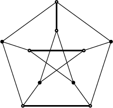
Theorem 2.3

Let $P$ be the Petersen graph, $Cl$ the Clebsch graph, $Gr$ the Grötsch graph, $D$ the dodecahedron (see Figure 2). Then $P\mathrel{\approx}_{{\mathbb{Z}}_{2}}Cl\mathrel{\approx}_{{\mathbb{Z}}_{2}}Gr\mathrel{\approx}_{{\mathbb{Z}}_{2}}D\mathrel{\approx}_{{\mathbb{Z}}_{2}}C_{5}$ . On the other hand, in the homomorphism order no two of these graphs are equivalent.

Proof

We have $C_{5}\subset P\subset Cl$ , $C_{5}\subset D$ , and $C_{5}\subset Gr$ . As inclusion is a homomorphism and hence it induces a $TT$ mapping, we only need to provide mappings $Cl\mathrel{\xrightarrow{TT}}C_{5}$ , $D\mathrel{\xrightarrow{TT}}C_{5}$ , and $Gr\mathrel{\xrightarrow{TT}}C_{5}$ . In Figure 2, we emphasize some edges in each graph. Let $G$ be the considered graph and $A\subseteq E(G)$ the set of bold edges. Put $A_{1}=A$ and let $A_{2}$ , $A_{3}$ , $A_{4}$ , $A_{5}$ denote the sets obtained from $A$ by rotation, so that the sets $A_{i}$ partition $E(G)$ . Define a mapping $E(G)\to E(C_{5})=\{e_{1},\dots,e_{5}\}$ by sending all edges in $A_{i}$ to $e_{i}$ .

Note that 4-edge subgraphs of $C_{5}$ generate its ${\mathbb{Z}}_{2}$ -tension space. Hence it is enough to verify that after deleting any color class we are left with a cut. Due to symmetry we only need to check that $E(G)\setminus A$ is a cut in $G$ . This is straightforward to verify, the corresponding bipartition of vertices is depicted in Figure 2. ∎

Graphs $\Delta(K_{n})$ will be further studied in Section 7. Here we only illustrate Theorem 2.2 by a particular choice $H=C_{5}$ . Graph $\Delta(H)$ consists of two components, each of which is isomorphic to the Clebsch graph $Cl$ . Hence, $G\mathrel{\xrightarrow{TT}}C_{5}$ is equivalent to $G\mathrel{\xrightarrow{hom}}Cl$ . This reproves part of Theorem 2.3 but, more importantly, this observation implicitly appeared in Reza, where a theorem of Gue was used to prove the following result.

Theorem 2.4

Any planar triangle-free graph admits a homomorphism to the Clebsch graph.

The next theorem gives an infinite class of graphs where homomorphisms and $TT$ mappings differ. In particular it implies that for every $n$ there are $n$ -connected graphs that are not homotens.

Theorem 2.5

Let $n$ be odd. Denote $G_{n}$ one of the (two isomorphic) components of $\Delta(K_{n})$ . Graphs $K_{n}$ and $G_{n}$ are $TT_{2}$ -equivalent and both are $(n-1)$ -connected. Finally, $G_{n}\mathrel{\thickspace\thickspace\not\negthickspace\negthickspace\xrightarrow{hom}}K_{n}$ for $n=2^{k}-1$ .

Proof

Using Theorem 2.2 for $G=H=K_{n}$ we get $K_{n}\mathrel{\xrightarrow{hom}}\Delta(K_{n})$ . From connectivity of $K_{n}$ and from Lemma 5 it follows $K_{n}\mathrel{\xrightarrow{TT_{2}}}G_{n}$ . Using Theorem 2.2 for $G=H=\Delta(K_{n})$ we get $\Delta(K_{n})\mathrel{\xrightarrow{TT_{2}}}K_{n}$ , hence also $G_{n}\mathrel{\xrightarrow{TT_{2}}}K_{n}$ .

Graph $K_{n}$ is $(n-1)$ -connected. Easily $\Delta(K_{n})=Q_{n}^{(2)}$ , where $Q_{n}$ is the $n$ -dimensional hypercube and $Q_{n}^{(2)}$ means that we are connecting by an edge the vertices at distance two in the hypercube. It is well-known and straightforward to verify that $Q_{n}$ is $(n-1)$ -connected. The vertices with odd (even) number of 1’s among their coordinates form the two components of $Q_{n}^{(2)}$ ; for an odd $n$ these two components are isomorphic by a mapping $\vec{x}\mapsto(1,1,\dots,1)-\vec{x}$ . Observe that if we take a path in $Q_{n}$ and leave every second vertex out, we obtain a path in $Q_{n}^{(2)}$ . So $Q_{n}^{(2)}$ is $(n-1)$ -connected since $Q_{n}$ is.

For the last part of the theorem, it follows from the remarks in the Section 7.2 that $\chi(G_{n})=n+1$ for $n=2^{k}-1$ . ∎

3 Density

3.1 A Ramsey-type theorem for locally balanced graphs

In this subsection we deal with undirected graphs only. We prove a Ramsey-type theorem that will be used in Section 3.2 as a tool to study $\mathrel{\prec}_{M}$ (on directed graphs).

An ordered graph is an undirected graph with a fixed linear ordering of its vertices. The ordering will be denoted by $<$ , an ordered graph by $(G,<)$ , or shortly by $G$ . We say that two ordered graphs are isomorphic, if the (unique) order-preserving bijection is a graph isomorphism. An ordered graph $(G,<)$ is said to be a subgraph of $(H,<^{\prime})$ , if $G$ is a subgraph of $H$ , and the two orderings coincide on $V(G)$ .

A circuit $C=v_{1},\dots,v_{l}$ in an ordered graph is balanced iff

|\{i;v_{i}<v_{(i\bmod l)+1}\}|=|\{i;v_{i}>v_{(i\bmod l)+1}\}|\,.

This can be reformulated using the notion preceding Lemma 3. Let $\myarrow{G}$ be a directed graph with $V(\myarrow{G})=V(G)$ and $E(\myarrow{G})=\{(u,v);\mbox{$uv\in E(G)$ and $u<v$}\}$ . (We can say that all edges are oriented “up”.) Then a circuit in $G$ is balanced iff the corresponding circuit in $\myarrow{G}$ is ${\mathbb{Z}}$ -balanced. Note that a circuit in $\myarrow{G}$ is ${\mathbb{Z}}_{2}$ -balanced iff its length is even.

Denote by $\mathop{\rm Cyc}_{p}$ the set of all ordered graphs that contain no odd circuit of length at most $p$ . Denote by $\mathop{\rm Bal}_{p}$ the set of all ordered graphs that contain no unbalanced circuit of length at most $p$ .

Nešetřil and Rödl (NR) proved the following Ramsey-type theorem.

Theorem 3.1

Let $k$ , $p$ be positive integers. For any ordered graph $(G,<)\in\mathop{\rm Cyc}_{p}$ there is an ordered graph $(H,<)\in\mathop{\rm Cyc}_{p}$ with the “Ramsey property”: for every coloring of $E(H)$ by $k$ colors there is a monochromatic subgraph ${(G^{\prime},<)}$ , isomorphic to $(G,<)$ .

We will need a version of this theorem for $\mathop{\rm Bal}_{p}$ . By the discussion above, this means that we consider ${\mathbb{Z}}$ -balanced (instead of ${\mathbb{Z}}_{2}$ -balanced) circuits.

Theorem 3.2

Let $r$ , $p$ be positive integers. For any ordered graph $(G,<)\in\mathop{\rm Bal}_{p}$ there is an ordered graph $(H,<)\in\mathop{\rm Bal}_{p}$ with the “Ramsey property”: for every edge coloring of $H$ by $r$ colors there is a monochromatic subgraph ${(G^{\prime},<)}$ , isomorphic to $G$ . This conclusion will be shortly written as $(H,<)\to(G,<)^{2}_{r}$ .

Proof

The proof of Theorem 3.2 uses a variant of the amalgamation method (partite construction) due to the first author and Rödl (see e.g. NR-Ramsey, Nes-Ramsey), which has many applications in structural Ramsey theory.

For the purpose of this proof we slightly generalize the notion of ordered graph. We work with graphs with a quasiordering $\leq$ of its vertices; such graphs are called quasigraphs, $\leq$ is called the standard ordering of $G$ . Alternatively, a quasigraph $(G,\leq)$ is a graph $G=(V,E)$ with a partition $V_{1}\cup V_{2}\cup\cdots\cup V_{a}$ of $V$ : each $V_{i}$ is a set of mutually equivalent vertices of $V$ and $V_{1}<V_{2}<\cdots<V_{a}$ . The number $a$ of equivalence classes of $\leq$ will be fixed throughout the whole proof. In this case we speak about $a$ -quasigraphs. It will be always the case that every $V_{i}$ is an independent set of $G$ .

An embedding $f:(G,\leq)\to(G^{\prime},\leq^{\prime})$ is an embedding (i.e. an isomorphism onto an induced subgraph) $G\to G^{\prime}$ which is moreover monotone with respect to the standard orderings $\leq$ and $\leq^{\prime}$ . Explicitly, such an embedding $f$ is an embedding of $G$ to $G^{\prime}$ for which there exists an increasing mapping $\iota:\{1,2,\dots,a\}\to\{1,2,\dots,a^{\prime}\}$ such that $f(V_{i})\subseteq V^{\prime}_{\iota(i)}$ for $i=1,\dots,a$ . (Here $V^{\prime}_{1}<V^{\prime}_{2}<\cdots<V^{\prime}_{a^{\prime}}$ are equivalence classes of the quasiorder $\leq^{\prime}$ .) By identifying the equivalent vertices of a quasigraph $G$ we get a graph $\bar{G}$ and a homomorphism $\pi:G\to\bar{G}$ ; graph $\bar{G}$ is called the shadow of $G$ , mapping $\pi$ is called shadow projection.

We prove Theorem 3.2 by induction on $p$ . The case $p=1$ is the Ramsey theorem for ordered graphs and so we can use Theorem 3.1 for $p=1$ . In the induction step ( $p\to p+1$ ) consider arbitrary ordered graph $(G,\leq)$ , let $G=(V,E)$ , $|V|=n$ , and $G\in\mathop{\rm Bal}_{p+1}$ . By the induction assumption there exists an ordered graph $(K,\leq)\in\mathop{\rm Bal}_{p}$ such that

K\to(G)_{r}^{2}\,.

Let $V(K)=\{x_{1}<\cdots<x_{a}\}$ and $E(K)=\{e_{1},\dots,e_{b}\}$ . In this situation we shall construct (by induction) $a$ -quasigraphs $P^{0}$ , $P^{1}$ , …, $P^{b}$ (called usually “pictures”). Then the quasigraph $P^{b}$ will be transformed to the desired ordered graph $(H,\leq)\in\mathop{\rm Bal}_{p}$ satisfying

(H,\leq)\to(G,\leq)_{r}^{2}\,.

We proceed as follows. Let $(P^{0},\leq^{0})\in\mathop{\rm Bal}_{p+1}$ be $a$ -quasiordered graph for which for every induced subgraph $G^{\prime}$ of $K$ , such that $(G^{\prime},\leq)$ is isomorphic to $(G,\leq)$ , there exists a subgraph $G_{0}$ of $P^{0}$ with the shadow $G^{\prime}$ . Clearly $(P^{0},\leq^{0})$ exists, as it can be formed by a disjoint union of $\binom{a}{n}$ copies of $G$ with an appropriate quasiordering.

In the induction step $k\to k+1$ ( $k\geq 0$ ) let the picture $(P^{k},\leq^{k})$ be given. Write $P^{k}=(V^{k},E^{k})$ and let $V_{1}^{k}<V_{2}^{k}<\cdots<V_{a}^{k}$ be all equivalence classes of $\leq^{k}$ . Consider the edge $e_{k+1}=\{x_{i_{k+1}},x_{j_{k+1}}\}$ of $K$ ( $x_{i_{k+1}}<x_{j_{k+1}}$ ). To simplify the notation, we will write $i=i_{k+1}$ , $j=j_{k+1}$ . Let $B^{k}=(V^{k}_{i}\cup V^{k}_{j},F^{k})$ be the bipartite subgraph of $P^{k}$ induced by the set $V^{k}_{i}\cup V^{k}_{j}$ . We shall make use of the following lemma.

Lemma 8

For every bipartite graph $B$ there exists a bipartite graph $B^{\prime}$ such that

B^{\prime}\to(B)_{r}^{2}\,.

(The embeddings of bipartite graphs map the upper part to the upper part and the lower part to the lower part.)

This lemma is easy to prove and it is well-known, see e.g. Nes-Ramsey.

Continuing our proof, let

B^{\prime k}\to(B^{k})_{r}^{2}

(1)

be as in Lemma 8 and put explicitly $B^{\prime k}=(V_{i}^{k+1}\cup V_{j}^{k+1},F^{k+1})$ . Let also ${\cal B}_{k}$ be the set of all induced subgraphs of $B^{\prime k}$ , which are isomorphic to $B^{k}$ . Now we are in the position to construct the picture $(P^{k+1},\leq^{k+1})$ .

We enlarge every copy of $B^{k}$ to a copy of $(P^{k},\leq^{k})$ while keeping the copies of $P^{k}$ disjoint outside the set $V_{i}^{k+1}\cup V_{j}^{k+1}$ . The quasiorder $\leq^{k+1}$ is defined from copies of quasiorder $\leq^{k}$ by unifying the corresponding classes. While this description perhaps suffices to many here is an explicit definition of $P^{k+1}$ :

Put $P^{k+1}=(V^{k+1},E^{k+1})$ , where $V^{k+1}=V^{k}\times{\cal B}/{\sim}$ . The equivalence $\sim$ is defined by

(v,B)\sim(v^{\prime},B^{\prime})\quad\Longleftrightarrow\quad v=v^{\prime}\in V_{i}^{k+1}\cup V_{j}^{k+1}\quad\hbox{or $\quad v=v^{\prime}$ and $B=B^{\prime}$.}

Denote by $[v,B]$ the equivalence class of $\sim$ containing $(v,B)$ . We define the edge set by putting $\{[v,B],[v^{\prime},B^{\prime}]\}\in E^{k+1}$ if $\{v,v^{\prime}\}\in E^{k}$ and $B=B^{\prime}$ . Define quasiorder $\leq^{k+1}$ by putting

[v,B]\leq^{k+1}[v^{\prime},B^{\prime}]\Longleftrightarrow v\leq^{k}v^{\prime}\,.

It follows that $\leq^{k+1}$ has $a$ equivalence classes $V_{1}^{k+1}<\cdots<V_{a}^{k+1}$ . (Note that this is consistent with the notation of classes $V_{i}^{k+1}$ , $V_{j}^{k+1}$ of $B^{\prime k}$ .)

Continuing this way, we finally define the picture $(P^{b},\leq^{b})$ . Put $H=P^{b}$ and let $\leq$ be an arbitrary linear ordering that extends the non-symmetric part of the quasiorder $\leq^{b}$ . We claim that the graph $H$ has the desired properties. To verify this it suffices to prove:

(i)

$(H,\leq)\in\mathop{\rm Bal}_{p+1}$ and
(ii)

$(H,\leq)\to(G,\leq)_{r}^{2}$ .

The statement (i) will be implied by the following claim.

Claim

1.

$(P^{0},\leq^{0})\in\mathop{\rm Bal}_{p+1}$ .
2.

If $(P^{k},\leq^{k})\in\mathop{\rm Bal}_{p+1}$ , then ${(P^{k+1},\leq^{k+1})}\in\mathop{\rm Bal}_{p+1}$ .

Proof (of Claim)

The first part follows from the construction. In the second part, suppose that $P^{k+1}$ contains an unbalanced circuit $C=u_{1},u_{2},\dots,u_{l}$ of length $l\leq p+1$ . Let $\pi:V(P^{k+1})\to V(K)$ be the projection, that is for $u\in V_{s}^{k+1}$ we have $\pi(u)=x_{s}$ . From the construction it follows that $\pi$ is a homomorphism $P^{k+1}\mathrel{\xrightarrow{hom}}K$ , in other words that $K$ is the shadow of $P^{k+1}$ .

Consider the closed walk $C_{\pi}=\pi(u_{1}),\pi(u_{2}),\dots,\pi(u_{l})$ in $K$ . As $C_{\pi}$ is unbalanced closed walk, it contains an unbalanced circuit of length $l^{\prime}\leq l$ . Since $K\in\mathop{\rm Bal}_{p}$ , we have $l^{\prime}=l=p+1$ , that is $\pi(u_{1}),\dots,\pi(u_{p+1})$ are all distinct. Let $u_{s}=[v_{s},B_{s}]$ . If $B_{1}=B_{2}=\cdots=B_{l}$ , that is the whole $C$ is contained in one copy of $P^{k}$ , we have a contradiction as $P^{k}\in\mathop{\rm Bal}_{p+1}$ .

Now we use the construction of $P^{k+1}$ as an amalgamation of copies of $P^{k}$ : If $B_{t}\neq B_{t+1}$ (indices modulo $l$ ), then $\pi(u_{t})\in\{x_{i_{k+1}},x_{j_{k+1}}\}$ . As the vertices $\pi(u_{1}),\dots,\pi(u_{l})$ are pairwise distinct, this happens just for two values of $t$ . Consequently, the whole $C^{\prime}$ is contained in two copies of $P^{k}$ and there are indices $\alpha$ , $\beta$ such that $\pi(u_{\alpha})=x_{i_{k+1}}$ and $\pi(u_{\beta})=x_{j_{k+1}}$ .

The circuit $C$ is a concatenation of $P^{\prime}$ and $P^{\prime\prime}$ —two paths between $u_{\alpha}$ and $u_{\beta}$ , each of them properly contained in one copy of $P^{k}$ . No copy of $P^{k}$ contains whole $C$ , therefore both $P^{\prime}$ and $P^{\prime\prime}$ have at least two edges, hence at most $p-1$ edges. Let $\bar{P}^{\prime}$ , $\bar{P}^{\prime\prime}$ denote the shadows of $P^{\prime}$ and $P^{\prime\prime}$ . Both $\bar{P}^{\prime}\cup\{e_{k+1}\}$ and $\bar{P}^{\prime\prime}\cup\{e_{k+1}\}$ are closed walks in $K$ containing at most $p$ edges. As $K\in\mathop{\rm Bal}_{p}$ , both of them are balanced, so $C$ is balanced as well, a contradiction. ∎

We turn to the proof of statement (ii). We use a standard argument that is the core of the amalgamation method. Let $E(H)=E(P^{b})={\cal A}_{1}\cup\dots\cup{\cal A}_{r}$ be a fixed coloring. We proceed by backwards induction $b\to b-1\to\cdots$ and we prove that there exists a quasisubgraph $P_{0}^{k}$ of $P^{b}$ isomorphic to $P^{k}$ such that for any $l>k$ , any two edges of $P_{0}^{k}$ with shadow $e_{l}$ get the same color. This is easy to achieve using the Ramsey properties (1) of graphs $B^{\prime k}$ . Finally, we obtain a copy $P_{0}^{0}$ of $P^{0}$ in $P^{b}$ such that the color of any of its edges depends only on its shadow (in $K$ ). However $K\to(G)_{r}^{2}$ and as for any copy $G^{\prime}$ of $G$ in $K$ there exists a subgraph $G_{0}$ of $\bar{P}^{0}$ such that its shadow is $G^{\prime}$ we get that there exists a monochromatic copy of $G$ in $P^{b}$ . This concludes the proof. ∎

3.2 Density

In this section we prove the density of $TT_{M}$ order (for every abelian group $M$ ). For this we first prove the “Sparse Incomparability Lemma”, Lemma 9 (analogous statement for homomorphisms appears in NR-rigid). Although the proof follows similar path as in the homomorphism case, some steps are considerably harder; the main reason for this is the nonexistence of products in the category of tension-continuous mappings. To overcome this obstacle, we use the Ramsey-type theorem from the previous subsection.

Lemma 9

Let $M$ be an abelian group, let $l$ , $t\geq 1$ be integers. Let $G_{1}$ , $G_{2}$ , …, $G_{t}$ , $H$ be graphs such that $H\thickspace\not\negthickspace\xrightarrow{TT_{M}}G_{i}$ for every $i$ and $H\thickspace\not\negthickspace\xrightarrow{TT_{M}}\overrightarrow{K}_{2}$ . Then there is a graph $G^{\prime}$ such that

1.

$G^{\prime}\mathrel{\prec}_{M}H$ , moreover $G^{\prime}\mathrel{\prec_{h}}H$ ,
2.

all circuits in $G^{\prime}$ shorter than $l$ are $M$ -balanced, and
3.

$G^{\prime}\thickspace\not\negthickspace\xrightarrow{TT_{M}}G_{i}$ for every $i=1,\dots,t$ .

Proof

Choose an odd integer $p$ larger than $\max\{|E(H)|,l\}$ . Pick any linear ordering of $V(H)$ to make $H$ into an ordered graph $(H,<)$ and subdivide each edge to increase the girth. More precisely, we replace every edge $e$ of $H$ by an oriented path $P(e)=e_{1},e_{2},\dots,e_{p}$ ; the ordering of $V(H)$ is extended to the new vertices so, that $e_{j}$ goes up iff $j$ is odd, see Figure 3. When we do this for every edge of $H$ , we forget the orientation of the edges and let $(H^{\prime},<)$ denote the resulting ordered graph. It is $(H^{\prime},<)\in\mathop{\rm Bal}_{p}$ .

Put $r=\max_{i}|E(G_{i})|^{|E(H)|}$ . Using Theorem 3.2 we find a graph $(R,<)\mathop{\rm Bal}_{p}$ satisfying $(R,<)\to(H^{\prime},<)^{2}_{r}$ As every circuit of $(R,<)$ is balanced, it is also $M$ -balanced.

We orient all edges of $R$ up (that is towards the vertex larger in $<$ ), and set $G^{\prime}=H\times R$ (see Figure 3). Formally, $V(G^{\prime})=V(H)\times V(R)$ , and for edges $e=uv$ of $H$ and $e^{\prime}=u^{\prime}v^{\prime}$ of $R$ we have an edge from $(u,u^{\prime})$ to $(v,v^{\prime})$ (this edge will be denoted by $(e,e^{\prime})$ ).

Now $G^{\prime}\mathrel{\xrightarrow{TT_{M}}}R$ (as there is even a homomorphism—the projection), so by Lemma 3 there is no short $M$ -unbalanced circuit in $G^{\prime}$ . This gives part 2 of the statement. The other projection of $G^{\prime}$ gives $G^{\prime}\mathrel{\xrightarrow{TT_{M}}}H$ , and indeed even $G^{\prime}\mathrel{\xrightarrow{hom}}H$ . To prove part 1, we need to exclude the case $H\mathrel{\xrightarrow{TT_{M}}}G^{\prime}$ . If such a mapping exists, denote $\bar{H}$ its image in $G^{\prime}$ . It is easy to verify that $H\mathrel{\xrightarrow{TT_{M}}}\bar{H}$ . As $s>|E(H)|$ , there is no $M$ -unbalanced circuit in $\bar{H}$ , hence $\bar{H}\mathrel{\xrightarrow{TT_{M}}}\overrightarrow{K}_{2}$ . By composition we get $H\mathrel{\xrightarrow{TT_{M}}}\overrightarrow{K}_{2}$ , a contradiction. Hence $G^{\prime}\mathrel{\prec}_{M}H$ , and therefore $G^{\prime}\mathrel{\prec_{h}}H$ too. It remains to prove part 3.

For the contrary, suppose there is an index $i$ and a $TT_{M}$ mapping $f:G^{\prime}\mathrel{\xrightarrow{TT_{M}}}G_{i}$ . As $G^{\prime}=H\times R$ , this induces a coloring $c$ of edges of $R$ by elements of $E(G_{i})^{E(H)}$ (where $c(e^{\prime})$ sends $e$ to $f((e,e^{\prime}))$ ). As we have chosen $R$ to be a Ramsey graph for $H^{\prime}$ , there is a monochromatic copy of $H^{\prime}$ in $R$ . To ease the notation we will suppose this copy is just $H^{\prime}$ , let $g$ be the color of edges of $H^{\prime}$ . We will show that $g$ is a $TT_{M}$ mapping $H\to G_{i}$ , and this will be our desired contradiction.

We will use Lemma 7, hence for any flow $\varphi:E(H)\to M$ we need to show that $\varphi_{g}$ is a flow. Clearly it is enough to verify this for $\varphi$ being an elementary flow, as elementary flows generate the $M$ -flow space on $H$ . So let $C$ be a circuit in $H$ that is the support of $\varphi$ . The corresponding circuit $\bar{C}$ in $H\times R$ has edge set

E(\bar{C})=\bigcup\{\{e\}\times P(e),e\in E(C)\}\,.

Let $\bar{\varphi}$ be the elementary flow on $H\times R$ corresponding to $\varphi$ . Explicitly,

\bar{\varphi}:(e,e_{i})\mapsto\begin{cases}\varphi(e)&\hbox{if $i$ is odd,}\\ -\varphi(e)&\hbox{if $i$ is even.}\\ \end{cases}

As $H^{\prime}$ is $g$ -monochromatic, $f((e,e_{i}))=g(e)$ for every $i$ . Consequently $\varphi_{g}=\bar{\varphi}_{f}$ , so $\varphi_{g}$ is a flow. ∎

Theorem 3.3

Let $M$ be an abelian group, let $t\geq 0$ be an integer. Let $G$ , $H$ be graphs such that $G\mathrel{\prec}_{M}H$ and $H\thickspace\not\negthickspace\xrightarrow{TT_{M}}\overrightarrow{K}_{2}$ . Let $G_{1}$ , $G_{2}$ , …, $G_{t}$ be pairwise incomparable (in $\mathrel{\prec}_{M}$ ) graphs satisfying $G\mathrel{\prec}_{M}G_{i}\mathrel{\prec}_{M}H$ for every $i$ . Then there is a graph $K$ such that

1.

$G\mathrel{\prec}_{M}K\mathrel{\prec}_{M}H$ ,
2.

$K\thickspace\not\negthickspace\xrightarrow{TT}G_{i}\thickspace\not\negthickspace\xrightarrow{TT}K$ for every $i=1,\dots,t$ .

If in addition $G\mathrel{\xrightarrow{hom}}H$ then we have even $G\mathrel{\prec_{h}}K\mathrel{\prec_{h}}H$ .

Proof

Choose $l>\max\{|E(H)|,|E(G_{i})|,i=1,\dots,t\}$ . We use Lemma 9 to get a graph $G^{\prime}$ such that $G^{\prime}\thickspace\not\negthickspace\xrightarrow{TT}G_{i}$ and $G^{\prime}\thickspace\not\negthickspace\xrightarrow{TT}G$ ; then put $K=G+G^{\prime}$ . Easily $G\mathrel{\preccurlyeq}K\leq H$ and $K\thickspace\not\negthickspace\xrightarrow{TT}G_{i}$ , $K\thickspace\not\negthickspace\xrightarrow{TT}G$ (as $G^{\prime}$ has this property). It remains to show $F\thickspace\not\negthickspace\xrightarrow{TT}K$ for $F\in\{H,G_{1},\dots,G_{t}\}$ . Note that it is not enough to show $F\thickspace\not\negthickspace\xrightarrow{TT}G$ and $F\thickspace\not\negthickspace\xrightarrow{TT}G_{i}$ , we have to proceed more carefully.

So suppose we have an $TT_{M}$ mapping $f:F\mathrel{\xrightarrow{TT}}G+G^{\prime}$ . Pick an edge $e_{0}\in E(G)$ , and define $g:E(F)\to E(G)$ as follows:

g(e)=\begin{cases}f(e)&\text{if $f(e)\in E(G)$}\\ e_{0}&\text{otherwise.}\\ \end{cases}

We prove that $g$ is $TT_{M}$ which will be a contradiction. So let $\tau$ be an $M$ -tension on $G$ , we are to prove that $\tau g$ is an $M$ -tension on $F$ . By the choice of $l$ , graph $f(F)\cap G^{\prime}$ doesn’t contain an $M$ -unbalanced circuit (there is no that short unbalanced circuit in $G^{\prime}$ ), hence any constant mapping is an $M$ -tension. So we may choose a tension $\tau^{\prime}$ on $G+G^{\prime}$ that equals a constant $\tau(e_{0})$ on $f(F)\cap G^{\prime}$ and extends $\tau$ . Clearly $\tau g$ is the same function as $\tau^{\prime}f$ , hence it is a tension.

For the last part of statement of the theorem, $G\mathrel{\xrightarrow{hom}}G+G^{\prime}\mathrel{\xrightarrow{hom}}H$ follows immediately (using Lemma 9, part 1). If we had $H\mathrel{\xrightarrow{hom}}K$ or $K\mathrel{\xrightarrow{hom}}G$ , then by Lemma 5 the homomorphism induces a $TT_{M}$ mapping $H\mathrel{\xrightarrow{TT_{M}}}K$ (or $K\mathrel{\xrightarrow{TT_{M}}}G$ , respectively), a contradiction. ∎

To state Theorem 3.3 in a concise form we define open and closed intervals in order $\mathrel{\prec}$ . Let $(G,H)_{M}=\{G^{\prime}\mid G\mathrel{\prec}_{M}G^{\prime}\mathrel{\prec}_{M}H\}$ and $[G,H]_{M}=\{G^{\prime}\mid G\mathrel{\preccurlyeq}_{M}G^{\prime}\mathrel{\preccurlyeq}_{M}H\}$ . Similarly, define $(G,H)_{h}$ and $[G,H]_{h}$ —intervals in order $\mathrel{\prec_{h}}$ . Lemma 5 implies that $[G,H]_{h}\subseteq[G,H]_{M}$ for any group $M$ . On the contrary, none of the two possible inclusions between $(G,H)_{h}$ and $(G,H)_{M}$ is valid for every $G$ , $H$ . Therefore the additions in the following corollaries do indeed provide a strengthening, we will use this strengthening in Section 7.4.

Corollary 3

Suppose $G\mathrel{\prec}_{M}H$ and $H\thickspace\not\negthickspace\xrightarrow{TT_{M}}\overrightarrow{K}_{2}$ . Then $(G,H)_{M}$ is nonempty. If in addition $G\mathrel{\prec_{h}}H$ then $(G,H)_{M}\cap(G,H)_{h}$ is nonempty.

Corollary 4

Suppose $G\mathrel{\prec}_{M}H$ and $H\thickspace\not\negthickspace\xrightarrow{TT_{M}}\overrightarrow{K}_{2}$ . Then any finite antichain of $\mathrel{\prec}_{M}$ restricted to $(G,H)$ can be extended. If in addition $G\mathrel{\prec_{h}}H$ then any finite antichain of $\mathrel{\prec}_{M}$ restricted to $(G,H)_{M}\cap(G,H)_{h}$ can be extended.

Remark 1

Throughout this section we need to assume $H\mathrel{\succ}_{M}\overrightarrow{K}_{2}$ : for example in Corollary 3 there is no graph $K$ satisfying $K_{1}\mathrel{\prec}_{M}K\mathrel{\prec}_{M}\overrightarrow{K}_{2}$ (if $K$ has no edge then it maps to $K_{1}$ , otherwise $\overrightarrow{K}_{2}$ maps to it). We may say that $(K_{1},\overrightarrow{K}_{2})$ is a gap.

If $M={\mathbb{Z}}_{2}$ all results of this section hold for undirected graphs, too, as all orientations of an undirected graph are $TT_{2}$ -equivalent.

Remark 2

If $M$ is finite we can prove Lemma 9 easily by using the construction $\Delta(G)$ (and its variant for general group $M$ ). For details, see NS.

4 Universality of $TT_{2}$ order

In this section we restrict our attention to $TT_{2}$ mappings and consequently to undirected graphs. We first construct a particular $TT_{2}$ -rigid graph. (By Corollary 6 such graph exists, but we need some additional properties.) Then we use this graph to provide a faithful functor from the category of homomorphisms to the category of $TT_{2}$ mappings.

Lemma 10

Let $S$ be the graph in Figure 4.

1.

$S$ is $TT_{2}$ -rigid, i.e. the only $TT_{2}$ mapping $S\to S$ is the identity.
2.

Suppose $G$ is a graph that contains edge-disjoint copies of $S$ : $S_{1}$ , …, $S_{t}$ . Suppose $G$ does not contain triangles nor pentagons, except those pentagons that are contained in some $S_{i}$ . Then the only $TT_{2}$ mapping $S\to G$ is the identity mapping to some $S_{i}$ .

Proof

We will prove the second part, which implies the first (by taking $G=S$ ). Consider a $TT_{2}$ mapping $f:S\to G$ . Let pentagons in $S$ be denoted $C^{1}$ , …, $C^{9}$ as in the figure, note that there are no other pentagons in $S$ . As there are no triangles in $G$ and the only pentagons are contained in some $S_{k}$ , we can deduce by Lemma 7 that each $C^{i}$ maps to a pentagon in some $S_{k}$ (possibly different $k$ for different $i$ ).

Pentagon $C^{i}$ shares an edge with $C^{j}$ iff $i$ and $j$ differ by 1 (modulo 9). As sharing an edge is preserved by any mapping and since different copies of $S$ in $G$ are edge-disjoint, we conclude that there is a copy of $S$ in $G$ (to simplify the notation, we will identify this copy with $S$ ) and a bijection $p:[9]\to[9]$ such that $f(C^{i})=C^{p(i)}$ for each $i$ ; moreover $p$ preserves the cyclic order. Next we note that the size of the intersection of neighbouring pentagons is preserved too. There are exactly three pairs of pentagons that share two edges: $\{C^{1},C^{2}\}$ , $\{C^{3},C^{4}\}$ , $\{C^{6},C^{7}\}$ . As the pairs $\{C^{1},C^{2}\}$ and $\{C^{3},C^{4}\}$ are adjacent, the pairs $\{C^{5},C^{6}\}$ and $\{C^{3},C^{4}\}$ have a common neighbouring pentagon, while the pairs $\{C^{5},C^{6}\}$ and $\{C^{1},C^{2}\}$ do not, we see that $p$ is the identity; that is $f(C^{i})=C^{i}$ for each $i$ .

We still have to prove that $f$ does not permute edges in the respective pentagons. Let $C^{o}$ be the outer cycle and note it is the only 9-cycle in $S$ that shares exactly one edge with each $C^{i}$ . Hence, $f$ is an identity on $E(C^{o})$ . This means that $f$ can only permute two edges that share an endpoint of some of the edges $a$ , $b$ , and $c$ .

Edge $a$ is a part of a 7-cycle $C^{a}$ that has four edges in common with $C^{o}$ . Now, $C^{o}$ is preserved by $f$ , and there is no other 7-cycle in $S$ with the same intersection with $C^{o}$ . Thus, $C^{a}$ is preserved as well, in particular $a$ and the edges incident with it are preserved. Edge $b$ is a part of a 7-cycle $C^{b}$ that intersects $C^{5}$ , $C^{6}$ , $C^{7}$ , $C^{8}$ and $C^{9}$ . Since the edges it has in common with $C^{6}$ , $C^{7}$ , and $C^{8}$ are preserved by $f$ (at least set-wise), and there is no other 7-cycle including these edges, $C^{b}$ is preserved too, in particular $b$ and the edges incident with it are preserved. Similarly, $c$ is contained in an $8$ -cycle that has five of its edges fixed, hence it is fixed by $f$ . ∎

Theorem 4.1

There is a mapping $F$ that assigns (undirected) graphs to (undirected) graphs, such that for any graphs $G$ , $H$ (we stress that we consider loopless graphs only) holds

G\mathrel{\xrightarrow{hom}}H\iff F(G)\mathrel{\xrightarrow{TT_{2}}}F(H)\,.

Moreover $F$ can be extended on mappings between graphs: if $f:G\to H$ is a homomorphism, then $F(f):F(G)\to F(H)$ is a $TT$ mapping and any $TT$ mapping between $F(G)$ and $F(H)$ is equal to $F(f)$ for some homomorphism $f:G\mathrel{\xrightarrow{hom}}H$ . (In category-theory terms $F$ is an embedding of the category of all graphs and their homomorphisms into the category of all graphs and all $TT_{2}$ -mappings between them.)

Proof

Let $S$ be the graph from Lemma 10, let $p$ , $q$ , $r$ , $s$ be its vertices as denoted in Figure 4. For a graph $G$ , let the vertices of $F(G)$ be $(V(G)\times V(S))\mathbin{\dot{\cup}}(E(G)\times\{1,2\})$ . On each set $\{v\}\times V(S)$ we place a copy of $S$ , it will be denoted by $S_{v}$ . For an edge $uv$ of $G$ we introduce edges $(u,p)(v,q)$ , $(u,q)(v,p)$ (we refer to them as to add-on edges) and paths of length two from $(u,r)$ to $(v,s)$ and from $(u,s)$ to $(v,r)$ (we refer to these as to add-on paths, the middle vertices of these paths are $(uv,1)$ and $(uv,2)$ ). There are no other edges in $F(G)$ . See Figure 5 for an example of the construction. As we wish to apply Lemma 10, we first show that $F(G)$ contains no triangles and only those pentagons that are contained in some $S_{v}$ . Suppose $C$ is a cycle violating this. If $C$ contains some add-on path, it is easy to check that the length of $C$ is at least six. If it is not then $C$ has to contain some add-on edges (as $S$ is triangle-free). If it contains only add-on edges and copies of the edge $pq$ then it has even length; otherwise it has length at least seven.

It is clear how to define $F(f)$ for a homomorphism $f:G\to H$ — $F(f)$ maps each $S_{v}$ in $G$ to $S_{f(v)}$ in $H$ in the only way, the edges between different copies of $S$ are mapped in the “canonical” way. Clearly $F(f)$ is a $TT$ mapping induced by a homomorphism.

The only difficult part is to show, that for every $g:F(G)\mathrel{\xrightarrow{TT}}F(H)$ there is an $f:G\mathrel{\xrightarrow{hom}}H$ such that $g=F(f)$ . So let $g$ be such a mapping. By Lemma 10 each copy of $S$ is mapped to a copy of $S$ , to be precise, there is a mapping $f:V(G)\to V(H)$ such that $g$ maps $S_{v}$ to $S_{f(v)}$ . Let $uv$ be an edge of $G$ . First, we show that $f(u)\neq f(v)$ . Suppose the contrary and consider the 7-cycle $(u,p)$ , $(u,q)$ , $(u,r)$ , $(u,s)$ , $x$ , $(v,r)$ , $(v,q)$ ( $x$ is the middle vertex of an add-on path). Since $S$ is rigid, edges $(u,q)(u,r)$ and $(v,q)(v,r)$ map to the same edge, hence the algebraical image of the other five edges is a cycle. However, there is no cycle of length at most five containing edges $pq$ and $rs$ , a contradiction.

Considering again the image of the same cycle shows that $f(u)$ and $f(v)$ are connected by an edge of $H$ , which finishes the proof. ∎

Remark 3

It is interesting to note that graphs $F(G)$ are all triangle-free. We believe that the construction from Theorem 4.1 can be modified to work for other groups than ${\mathbb{Z}}_{2}$ , some modification can possibly produce even graphs of girth at least $g$ , for any given $g$ . If we consider graphs containing complete graphs then the situation becomes easier. In fact (as we show in the next section), $TT$ mappings coincide with homomorphisms on a large class of graphs (called nice graphs)—see Theorem 5.1 and the discussion below it.

5 Random graphs and $TT$ mappings

In this section we investigate cut-continuous, i.e. $TT_{2}$ mappings, only; that is we restrict our attention to the case $M={\mathbb{Z}}_{2}$ and to undirected graphs. We study whether typically (in the sense of random graphs) a $TT_{2}$ mapping is induced by a homomorphism. Recall, that a graph $G$ is said to be homotens if for any graph $H$ any $TT_{2}$ mapping $G\mathrel{\xrightarrow{TT_{2}}}H$ is induced by a homomorphism. The main result of this section is that most graphs are homotens.

We consider the random graph model ${\mathbb{G}}_{n}$ , that is every graph with vertices $\{1,2,\dots,n\}$ has the same probability (although some of the results can be modified for other models too). As it is usual in the random graph setting, we study whether some graph property $P$ holds almost surely (a.s.), that is whether

\lim_{n\to\infty}Pr_{G\in{\mathbb{G}}_{n}}[\mbox{$G$ has $P$}]=1\,.

We start with a useful notion that will help us to handle $TT$ mappings (see Theorem 5.1). We call a graph $G$ nice if the following holds

1.

every edge of $G$ is contained in some triangle
2.

every triangle in $G$ is contained in some copy of $K_{4}$
3.

every copy of $K_{4}$ in $G$ is contained in some copy of $K_{5}$
4.
for every $K$ , $K^{\prime}$ that are copies of $K_{4}$ in $G$ there is a sequence of vertices $v_{1}$ , $v_{2}$ , …, $v_{t}$ such that
- •
  
  $V(K)=\{v_{1},v_{2},v_{3},v_{4}\}$ ,
- •
  
  $V(K^{\prime})=\{v_{t},v_{t-1},v_{t-2},v_{t-3}\}$ ,
- •
  
  $v_{i}v_{j}$ is an edge of $G$ whenever $1\leq i<j\leq t$ and $j\leq i+3$ .

Lemma 11

Let $f:K_{5}\mathrel{\xrightarrow{TT}}H$ , where $H$ is any loopless graph. Then $f$ is induced by an injective homomorphism (that is, by an embedding). Moreover, this isomorphism is uniquely determined.

Proof

Suppose $f(K_{5})$ is a four-colorable graph. A composition of $TT$ mapping $f:K_{5}\to f(K_{5})$ with a $TT$ mapping induced by a homomorphism $f(K_{5})\to K_{4}$ gives $K_{5}\mathrel{\xrightarrow{TT}}K_{4}$ . Consider three cuts of size 4 in $K_{4}$ ; they cover every edge exactly twice. Hence, their preimages are three cuts in $K_{5}$ that cover every edge exactly twice. But $K_{5}$ has 20 edges, while the largest cut has only $2\cdot 3=6$ edges.

Hence, chromatic number of $f(K_{5})$ is at least five. As it has at most 10 edges, the chromatic number is exactly five. Let $V_{1}$ , …, $V_{5}$ be the color classes. There is exactly one edge between two distinct color classes (otherwise the graph is four-colorable). Hence, $f$ is a bijection. Next, $|V_{i}|=1$ for every $i$ (as otherwise, we can split one color-class to several pieces and join these to the other classes; again, the graph would be four-colorable). Consequently, $f(K_{5})$ is isomorphic to $K_{5}$ .

We call star a set of edges sharing a vertex. We know that preimage of every star is a star, hence as $f$ is a bijection, also image of every star is a star. Stars sharing an edge map to stars sharing an edge, hence $f$ is induced by a homomorphism. ∎

Theorem 5.1

Let $G$ be a nice graph, let $f:G\mathrel{\xrightarrow{TT}}H$ . Then $f$ is induced by a homomorphism. Shortly, every nice graph is homotens.

Proof

Let $K$ be a copy of $K_{5}$ in $G$ . By Lemma 11 the restriction of $f$ to $K$ is induced by a homomorphism, let it be denoted by $h_{K}$ . If $K$ is a copy of $K_{4}$ in $G$ , by the third condition from the definition of nice it is contained in some $K^{\prime}$ —copy of $K_{5}$ . The restriction $h_{K}=h_{K^{\prime}}|_{K}$ induces $f$ on $K$ ; clearly such $h_{K}$ is unique (it does not depend on the choice of $K^{\prime}$ ).

As every edge is contained in some copy of $K_{4}$ , it is enough to prove that there is a common extension of all homomorphisms $\{h_{K}\mid K\subseteq G,\ K\simeq K_{4}\}$ (we may define it arbitrarily on the isolated vertices of $G$ ).

We say that $h_{K}$ and $h_{K^{\prime}}$ agree if for any $v\in V(K)\cap V(K^{\prime})$ we have $h_{K}(v)=h_{K^{\prime}}(v)$ . Thus, we need to show that any two homomorphisms $h_{K}$ , $h_{K^{\prime}}$ ( $K\simeq K^{\prime}\simeq K_{4}$ ) agree.

Let first $K$ , $K^{\prime}$ be copies of $K_{4}$ that intersect in a triangle. Then $h_{K}$ and $h_{K^{\prime}}$ agree (note that this does not necessarily hold if the intersection is just an edge).

Now suppose $K$ , $K^{\prime}$ are copies of $K_{4}$ that have a common vertex $v$ . Since $G$ is nice, we find $v_{1}$ , $v_{2}$ , …, $v_{t}$ as in the definition. Let $K_{i}=G[\{v_{i},v_{i+1},v_{i+2},v_{i+3}\}]$ ; every $K_{i}$ is a copy of $K_{4}$ , $K_{1}=K$ and $K_{t-3}=K^{\prime}$ . Suppose $v=v_{l}=v_{r}$ , where $l\in\{1,2,3,4\}$ , $r\in\{t-3,t-2,t-1,t\}$ . Consider a closed walk $W=v_{l},v_{l+1},\dots,v_{r-1},v_{r}$ . Let $v^{\prime}_{i}=h_{K_{i}}(v_{i})$ for $l\leq i\leq r-3$ and $v^{\prime}_{i}=h_{K_{r-3}}(v_{i})$ for $r-3\leq i\leq r$ . Homomorphisms $h_{K_{i}}$ and $h_{K_{i+1}}$ agree, hence $v^{\prime}_{i}v^{\prime}_{i+1}=f(v_{i}v_{i+1})$ is an edge of $H$ . So $W^{\prime}=v^{\prime}_{l},v^{\prime}_{l+1},\dots,v^{\prime}_{r-1},v^{\prime}_{r}$ .

Let $\varphi(e)$ be the number of occurrences of $e$ in $W$ taken modulo 2. Clearly $\varphi$ is a ${\mathbb{Z}}_{2}$ -flow. Similarly, define $\varphi^{\prime}(e)$ as the number of occurrences of $e$ in $W^{\prime}$ taken modulo 2. We have $\varphi^{\prime}=\varphi_{f}$ , hence by Lemma 7 $\varphi^{\prime}$ is a flow. This can happen only if $W^{\prime}$ is a closed walk, that is $v^{\prime}_{l}=v^{\prime}_{r}$ .

By definition, $v^{\prime}_{r}=h_{K^{\prime}}(v)$ . As mappings $h_{K_{i}}$ and $h_{K_{i+1}}$ agree, we have that $h_{K_{i}}(v_{i+3})=h_{K_{i+3}}(v_{i+3})$ . Consequently, $v^{\prime}_{l}=h_{K}(v)$ , which finishes the proof. ∎

Let us remark that Theorem 5.1 may be used to prove Theorem 4.1 in a different way. To do this, it suffices to modify the replacement operation (HN) in such a way that the resulting graph $F(G)$ is nice. (See HN for a nice example of a nice rigid graph.)

Consider the countable random graph ${\mathbb{G}}_{\omega}$ . Surprisingly, it is almost surely isomorphic to a particular graph, the so-called Rado graph. This is a remarkable graph (it is homogeneous and it contains every countable graph as an induced subgraph), see Cameron for more detailed discussion.

Lemma 12

Random graph from ${\mathbb{G}}_{n}$ is almost surely nice. The Rado graph is nice.

Proof

We prove the first statement, the second is proved in exactly the same way, except we do not have to take the limit.

For $S\subseteq V(G)$ (where $G={\mathbb{G}}_{n}$ ) write $C_{S}$ for the event, that there is a common neighbor for all vertices in $S$ . If $|S|=4$ , clearly the probability of $C_{S}$ is $(1-\frac{1}{2^{s}})^{n-s}$ . As $\binom{n}{s}\cdot(1-\frac{1}{2^{s}})^{n-s}$ tends to zero for any fixed $s$ , $C_{S}$ holds a.s. for all $S$ with size at most 4. This implies the first three conditions on $G$ .

To prove the last condition, let $K$ , $K^{\prime}$ be two copies of $K_{4}$ . Denote vertices of $K$ by $v_{1}$ , $v_{2}$ , $v_{3}$ , $v_{4}$ , and vertices of $K^{\prime}$ by $v_{8}$ , $v_{9}$ , $v_{10}$ , $v_{11}$ (in any order). If we find a triangle that is connected to every vertex in $K\cup K^{\prime}$ , we may denote its vertices by $v_{5}$ , $v_{6}$ , $v_{7}$ and we are done. For a given three-element set $S\subseteq V(G)\setminus(V(K)\cup V(K^{\prime}))$ the probability that $S$ induces a triangle and is connected to all vertices in $V(K)\cup V(K^{\prime}))$ is at least $2^{-21}$ , hence the probability that there is no such $S$ is at most $(1-2^{-21})^{n-6/3}$ . As the number of possible pairs $(K,K^{\prime})$ is $O(n^{8})$ , this concludes the proof. ∎

Lemma 13

The complete graph $K_{n}$ is nice whenever $n\geq 5$ .

Proof

The straightforward verification is left to the reader. ∎

From Theorem 5.1, Lemma 12, and Lemma 13 we immediately get the following corollary (a different proof of $K_{4}\mathrel{\prec}K_{5}\mathrel{\prec}\cdots$ is given in LMT).

Corollary 5

1.

Random graph from ${\mathbb{G}}_{n}$ is almost surely homotens.
2.

The Rado graph is homotens.
3.

The complete graph $K_{n}$ is homotens whenever $n\geq 5$ . In particular, in the $TT_{2}$ order we have

$K_{3}\mathrel{\approx}K_{4}\mathrel{\prec}K_{5}\mathrel{\prec}K_{6}\mathrel{\prec}K_{7}\mathrel{\prec}\cdots\,.$

Corollary 5 enables us to prove a $TT$ version of the following result about homomorphisms of random graphs. (The original theorem appears in KR, see also Section 3.6 of HN.)

Theorem 5.2 (KR)

Random graph is almost surely rigid (with respect to homomorphism). There are

\frac{1}{n!}\binom{\binom{n}{2}}{\left\lfloor\frac{1}{2}\binom{n}{2}\right\rfloor}(1-o(1))

graphs on $n$ vertices with no homomorphism between any two of them and with only identical homomorphism on each of them.

Corollary 6

Random graph is almost surely $TT$ -rigid. There are

\frac{1}{n!}\binom{\binom{n}{2}}{\left\lfloor\frac{1}{2}\binom{n}{2}\right\rfloor}(1-o(1))

pairwise $TT$ -incomparable $TT$ -rigid graphs on $n$ vertices.

Remark 4

The method of this section may be used for $M\neq{\mathbb{Z}}_{2}$ as well. In fact, if $M$ is not a power of ${\mathbb{Z}}_{2}$ , we can prove analogy of Lemma 11 for $K_{4}$ . Then we can prove stronger version of Theorem 5.1—for any group $M$ , a nice graph is $M$ -homotens; we can even slightly weaken the definition of “nice” if $M$ is not a power of ${\mathbb{Z}}_{2}$ . Similarly, we can generalize other results of this section. For details, see NS and RSthesis.

6 Influence of the group

In this section we study how the notion of $M$ -tension-continuous mapping depends on the group $M$ . Although the existence of $M$ -tension-continuous mappings seems to be strongly dependent on the choice of $M$ we prove here (in Theorem 6.2) that this dependence relates only to the cyclical structure of $M$ .

Throughout this section, $G$ , $H$ will be two graphs, $f:E(G)\to E(H)$ a mapping, and $M$ , $N$ groups, recall we consider only abelian groups (as is usual in the study of group-valued flows). As we are interested mainly in finite graphs, we can restrict our attention to finitely generated groups—clearly $f$ is $M$ -tension-continuous iff it is $N$ -tension-continuous for every finitely generated subgroup of $M$ .

Hence, we can use the classical characterization of finitely generated Abelian groups (see e.g. Lang).

Theorem 6.1

For a finitely generated abelian group $M$ there are integers $\alpha$ , $k$ , $\beta_{i}$ , $n_{i}$ ( $i=1,\dots,k$ ) so that

M\simeq{\mathbb{Z}}^{\alpha}\times\prod_{i=1}^{k}{\mathbb{Z}}_{n_{i}}^{\beta_{i}}\,.

(2)

For a group $M$ in the form (2), denote $n(M)=\infty$ if $\alpha>0$ , otherwise let $n(M)$ be the least common multiple of $\{n_{1},\dots,n_{k}\}$ .

As a first step to complete characterization we consider a specialized question: given a $TT_{M}$ mapping, when can we conclude that it is $TT_{N}$ as well?

Lemma 14

1.

If $f$ is $TT_{\mathbb{Z}}$ then it is $TT_{M}$ for any $M$ .
2.

Let $M$ be a subgroup of $N$ . If $f$ is $TT_{N}$ then it is $TT_{M}$ .

Proof

1. This appears as Theorem 4.4 in DNR.

2. Let $\tau$ be an $M$ -tension on $H$ . As $M\leq N$ , we may regard $\tau$ as an $N$ -tension, hence $\tau f$ is an $N$ -tension on $G$ . As it attains only values in the range of $\tau$ , hence in $M$ , it is an $M$ -tension, too. ∎

Lemma 15

Let $M_{1}$ , $M_{2}$ be two abelian groups. Mapping $f$ is $TT_{M_{1}}$ and $TT_{M_{2}}$ if and only if it is $TT_{M_{1}\times M_{2}}$ .

Proof

As $M_{1}$ , $M_{2}$ are subgroups of $M_{1}\times M_{2}$ , one implication follows from the second part of Lemma 14. For the other implication let $\tau$ be an $M_{1}\times M_{2}$ tension on $H$ . Write $\tau=(\tau_{1},\tau_{2})$ , where $\tau_{i}$ is an $M_{i}$ -tension on $H$ . By assumption, $\tau_{i}f$ is an $M_{i}$ tension on $G$ , consequently $\tau f=(\tau_{1}f,\tau_{2}f)$ is a tension too. ∎

The following (somewhat surprising) lemma shows that we can restrict our attention to cyclic groups only.

Lemma 16

1.

If $n(M)=\infty$ then $f$ is $TT_{M}$ if and only if it is $TT_{\mathbb{Z}}$ .
2.

Otherwise $f$ is $TT_{M}$ if and only if it is $TT_{n(M)}$ .

Proof

By previous lemmas. Note that ${\mathbb{Z}}_{n}$ is a subgroup of $\prod_{i=1}^{k}{\mathbb{Z}}_{n_{i}}^{\beta_{i}}$ . ∎

By a theorem of Tutte (see Diestel), the number of nowhere-zero flows on a given graph does depend only on the size of the group (that is, surprisingly, it does not depend on the structure of the group). Before proceeding in the main direction of this section, let us note a consequence of Lemma 16, which is an analogy of the Tutte’s theorem.

Theorem 6.2

Given graphs $G$ , $H$ , the number of $TT_{M}$ mappings from $G$ to $H$ depends only on $n(M)$ .

Lemma 16 suggests to define for two graphs the set

TT(G,H)=\{n\geq 1\mid\hbox{there is $f:E(G)\to E(H)$ such that $f$ is $TT_{n}$}\}

and for a particular $f:E(G)\to E(H)$

TT(f,G,H)=\{n\geq 1\mid\hbox{$f$ is $TT_{n}$}\}\,.

Remark that most of these sets contain 1: ${\mathbb{Z}}_{1}$ is a trivial group, hence any mapping is $TT_{1}$ . Therefore $1\in TT(f,G,H)$ for every $f:E(G)\to E(H)$ , while $1\in TT(G,H)$ iff there exists a mapping $E(G)\to E(H)$ . This happens precisely when $E(H)$ is nonempty or $E(G)$ is empty.

Lemma 17

Either $TT(f,G,H)$ is finite or $TT(f,G,H)={\mathbb{N}}$ . In the latter case $f$ is $TT_{\mathbb{Z}}$ .

Proof

It is enough to prove that $f$ is $TT_{\mathbb{Z}}$ if it is $TT_{n}$ for infinitely many integers $n$ . To this end, take a ${\mathbb{Z}}$ -tension $\tau$ on $H$ . As $\tau_{n}:e\mapsto\tau(e)\bmod n$ is a ${\mathbb{Z}}_{n}$ -tension, $\tau_{n}f=\tau f\bmod n$ is a ${\mathbb{Z}}_{n}$ -tension whenever $f$ is $TT_{n}$ . To show $\tau$ is a ${\mathbb{Z}}$ -tension consider a circuit $C$ and let $s$ be the “ $\pm$ -sum” (in ${\mathbb{Z}}$ ) along $C$ . As $s\bmod n=0$ for infinitely many values of $n$ , we have $s=0$ . ∎

Any $f$ induced by a homomorphism provides an example where $TT(f,G,H)$ is the whole ${\mathbb{N}}$ . For finite sets, the situation is more interesting. By the next theorem the sets $TT(f,G,H)$ are precisely ideals in the divisibility lattice.

Theorem 6.3

Let $T$ be a finite subset of ${\mathbb{N}}$ . Then the following are equivalent.

1.

There are $G$ , $H$ , $f$ such that $T=TT(f,G,H)$ .
2.

There is $n\in{\mathbb{N}}$ such that $T$ is the set of all divisors of $n$ .

Proof

First we show 1. implies 2. The set $T$ has the following properties

(i)

If $a\in T$ and $b|a$ then $b\in T$ . (We use the second part of Lemma 14: if $b$ divides $a$ , then ${\mathbb{Z}}_{b}\leq{\mathbb{Z}}_{a}$ .)
(ii)

If $a,b\in T$ then the least common multiple of $a$ , $b$ is in $T$ . (We use Lemma 14 and Lemma 15: if $l=\mathop{\rm lcm}\nolimits(a,b)$ then ${\mathbb{Z}}_{l}\leq{\mathbb{Z}}_{a}\times{\mathbb{Z}}_{b}$ .)

Denote $n$ the maximum of $T$ . By (i), all divisors of $n$ are in $T$ . If there is a $k\in T$ that does not divide $n$ then $\mathop{\rm lcm}\nolimits(k,n)$ is element of $T$ larger than $n$ , a contradiction.

For the other implication, let $f$ be the only mapping from $\myarrow{C}_{n}$ to $\overrightarrow{K}_{2}$ . Then $TT(f,\myarrow{C}_{n},\overrightarrow{K}_{2})=T$ : mapping $f$ is $TT_{k}$ iff for any $a\in{\mathbb{Z}}_{k}$ the constant mapping $E(\myarrow{C}_{n})\mapsto a$ is a ${\mathbb{Z}}_{k}$ -tension; this occurs precisely when $k$ divides $n$ . ∎

Let us turn to description of sets $TT(G,H)$ . Although we are working with finite graphs throughout the paper, we stress here that $G$ , $H$ are finite graphs—in contrary with most of other results, this one is not true for infinite graphs.

Lemma 18

Let $G$ , $H$ be finite graphs. Either $TT(G,H)$ is finite or $TT(G,H)={\mathbb{N}}$ . In the latter case $G\mathrel{\preccurlyeq}_{\mathbb{Z}}H$ .

Proof

As in the proof of Lemma 17, the only difficult step is to show that if $G\mathrel{\preccurlyeq}_{n}H$ for infinitely many values of $n$ , then $G\mathrel{\preccurlyeq}_{\mathbb{Z}}H$ . As $G$ and $H$ are finite, there is only a finite number of possible mappings between their edge sets. Hence, there is one of them, say $f:E(G)\to E(H)$ , that is $TT_{n}$ for infinitely many values of $n$ . By Lemma 17 we have $f:G\mathrel{\xrightarrow{TT_{{\mathbb{Z}}}}}H$ . ∎

When characterizing the sets $TT(G,H)$ we first remark that an analogue of Lemma 15 does not hold: there is a $TT_{M}$ mapping from $\myarrow{C}_{9}$ to $\myarrow{C}_{7}$ for $M={\mathbb{Z}}_{2}$ (mapping induced by a homomorphism of the undirected circuits) and for $M={\mathbb{Z}}_{3}$ (e.g. a constant mapping), but not the same mapping for both, hence there is no $TT_{{\mathbb{Z}}_{2}\times{\mathbb{Z}}_{3}}$ mapping. We will see that the sets $TT(G,H)$ are precisely down-sets in the divisibility poset. First, we prove a lemma that will help us to construct pairs of graphs $G$ , $H$ with a given $TT(G,H)$ . Integer cone of a set $\{s_{1},\dots,s_{t}\}\subseteq{\mathbb{N}}$ is the set $\{\sum_{i=1}^{t}a_{i}s_{i}\mid a_{i}\in{\mathbb{Z}},a_{i}\geq 0\}$ .

Lemma 19

Let $A$ , $B$ be non-empty subsets of ${\mathbb{N}}$ , $a\in{\mathbb{N}}$ , define $G=\bigcup_{a\in A}\myarrow{C}_{a}$ , and $H=\bigcup_{b\in B}\myarrow{C}_{b}$ . Then there is a $TT_{n}$ mapping from $G$ to $H$ if and only if

\hbox{$A$ is a subset of the integer cone of $B\cup\{n\}$}\,.

Proof

We use Lemma 7. Consider a flow $\varphi_{a}$ attaining value 1 on $\myarrow{C}_{a}$ and 0 elsewhere. Algebraical image of this flow is a flow, hence it is (modulo $n$ ) a sum of several flows along the cycles $\myarrow{C}_{b}$ , implying $a$ is in integer cone of $B\cup\{n\}$ . On the other hand if $a=\sum_{i}b_{i}+cn$ then we can map any $c$ edges of $\myarrow{C}_{a}$ to one (arbitrary) edge of $H$ , and for each $i$ any (“unused”) $b_{i}$ edges bijectively to $\myarrow{C}_{b_{i}}$ . After we have done this for each $a\in A$ we will have constructed a ${\mathbb{Z}}_{n}$ -tension-continuous mapping from $G$ to $H$ . ∎

Theorem 6.4

Let $T$ be a finite subset of ${\mathbb{N}}$ . Then the following are equivalent.

1.

There are $G$ , $H$ such that $T=TT(G,H)$ .
2.

There is a finite set $M\subset{\mathbb{N}}$ such that

$T=\{k\in{\mathbb{N}};(\exists m\in M)k|m\}\,.$

Proof

If $T$ is empty, we take $M$ empty. In the other direction, if $M$ is empty we just consider graphs such that $E(H)$ is empty and $E(G)$ is not. Next, we suppose $M$ is nonempty.

By the same reasoning as in the proof of Theorem 6.3 we see that if $a\in T$ and $b|a$ then $b\in T$ . Hence, 1 implies 2, as we can take $M=T$ (or, to make $M$ smaller, let $M$ consist of the maximal elements of $T$ in the divisibility relation).

For the other implication let $p>4\max M$ be a prime, let $p^{\prime}\in(1.25p,1.5p)$ be an integer. Let $A=\{p,p^{\prime}\}$ and

B=\{p-m;m\in M\}\cup\{p^{\prime}-m;m\in M\}\,;

note that every element of $B$ is larger than $\tfrac{3}{4}p$ . As in Lemma 19 we define $G=\bigcup_{a\in A}\myarrow{C}_{a}$ , $H=\bigcup_{b\in B}\myarrow{C}_{b}$ . We claim that $TT(G,H)=T$ . By Lemma 19 it is immediate that $TT(G,H)\supseteq T$ . For the other direction take $n\in TT(G,H)$ . By Lemma 19 again, we can express $p$ and $p^{\prime}$ in form

\sum_{i=1}^{t}b_{i}+cn

(3)

for integers $c,t\geq 0$ , and $b_{i}\in B$ .

•

If $t\geq 2$ then the sum in (3) is at least $1.5p$ ; hence neither $p$ nor $p^{\prime}$ can be expressed with $t\geq 2$ .
•
If $t=1$ then we distinguish two cases.
- $\bullet$
  
  $p=(p-m)+cn$ , hence $n$ divides $m$ and $n\in T$ .
- $\bullet$
  
  $p=(p^{\prime}-m)+cn$ , hence $p^{\prime}-p\leq m$ . But $p^{\prime}-p>0.25p>m$ , a contradiction.
Considering $p^{\prime}$ we find that either $n\in T$ or $p^{\prime}=(p-m)+cn$ .
•

Finally, consider $t=0$ . If $p=cn$ then either $n=1\in t$ or $n=p$ . (We don’t claim anything about $p^{\prime}$ .)

To summarize, if $n\in TT(G,H)\setminus T$ then necessarily $n=p$ . For $p^{\prime}$ we have only two possible expressions, $p^{\prime}=cn$ and $p^{\prime}=(p-m)+cn$ . We easily check that both of them lead to a contradiction. The first one contradicts $1.25p<p^{\prime}<1.5p$ . In the second expression $c=0$ implies $p^{\prime}<p$ while $c\geq 1$ implies $p^{\prime}\geq 2p-m\geq 1.75p$ , again a contradiction. ∎

Remark 5

This paper concentrates on $TT$ mappings. We remark, however, that the same proof yields a characterization of sets $XY(f,G,H)$ and $XY(G,H)$ for $XY\in\{FF,FT,TF\}$ (which are defined for $FF$ , $FT$ , and $TF$ mappings in the same way as sets $TT(f,G,H)$ and $TT(G,H)$ for $TT$ mappings).

7 Miscellanea

7.1 Complexity

Let $\mathop{\textsc{TT}}_{M}(H)$ denote the problem of decision, whether for a given graph $G$ there is a $TT_{M}$ mapping $G\mathrel{\xrightarrow{TT_{M}}}H$ . The complexity of the related problem $\mathop{\textsc{HOM}}(H)$ (that is the testing of the existence of a homomorphism to $H$ ) is now well understood, at least for undirected graphs: $\mathop{\textsc{HOM}}(H)$ is NP-complete if and only if $H$ contains an odd circuit, otherwise it is in P (as it is equivalent to decide whether $G$ is bipartite), see HN-complexity. In the same spirit, we wish to determine the complexity of the problem $\mathop{\textsc{TT}}_{M}(H)$ .

Theorem 7.1

Let $H$ be an undirected graph. Then $\mathop{\textsc{TT}}_{{\mathbb{Z}}_{2}}(H)$ is NP-complete if $H$ contains an odd circuit; otherwise it is polynomial.

Proof

By Theorem 2.2, problems $\mathop{\textsc{TT}}_{2}(H)$ and $\mathop{\textsc{HOM}}(\Delta(H))$ have the same answer for any graph $G$ , hence they have the same complexity. Observe that $\Delta(H)$ is bipartite iff $H$ is bipartite: $H$ and $\Delta(H)$ are $TT_{2}$ equivalent and any graph is bipartite iff it admits a $TT_{2}$ mapping to $\overrightarrow{K}_{2}$ . Consequently, $\mathop{\textsc{TT}}_{2}(H)$ is NP-complete iff $H$ contains an odd circuit.

For $M\neq{\mathbb{Z}}_{2}$ (or ${\mathbb{Z}}_{2}^{k}$ ), we may still reduce $\mathop{\textsc{TT}}_{M}(H)$ to $\mathop{\textsc{HOM}}(H^{\prime})$ for a suitable graph $H^{\prime}$ . However, now we deal with directed graphs, where the complexity of $\mathop{\textsc{HOM}}$ is not characterized. Another obstacle is that for $M={\mathbb{Z}}$ the graph $H^{\prime}$ is infinite. (For $H$ infinite, the complexity of $\mathop{\textsc{HOM}}(H)$ was investigated in BN.)

7.2 Codes and $\chi/\chi_{TT}$

In this section we first restate parts of LMT in our terminology. Inspired by the definition of $\chi(G)$ via homomorphisms we may define

\chi_{TT}(G)=\min\{n;G\mathrel{\xrightarrow{TT_{2}}}K_{n}\}\,.

For random graphs, Corollary 5 implies that $\chi_{TT}(G)=\chi(G)$ almost surely. For general graph $G$ , Lemma 5 implies $\chi_{TT}(G)\leq\chi(G)$ , on the other hand $\chi_{TT}(G)>\chi(G)/2$ follows from the fact that homomorphisms and $TT_{2}$ mappings to $K_{2^{k}}$ coincide (LMT, DNR). More precise information on behaviour of $\chi(G)/\chi_{TT}(G)$ is desirable.

Consequently, let ${\cal G}_{n}=\{G\mid G\mathrel{\xrightarrow{TT_{2}}}K_{n}\}$ and study $\chi(G)$ for $G\in{\cal G}_{n}$ . By Lemma 2.2, $G\in{\cal G}_{n}$ is equivalent to $G\mathrel{\xrightarrow{hom}}\Delta(K_{n})$ . In other words,

•

$\Delta(K_{n})\in{\cal G}_{n}$ ; and
•

for every $G\in{\cal G}_{n}$ we have $G\mathrel{\xrightarrow{hom}}\Delta(K_{n})$ .

This reduces the problem of behaviour of $\chi_{TT}(G)/\chi(G)$ to special values of $G$ .

Problem 2

Determine the limit of $\chi(\Delta(K_{n}))/n$ (and in particular decide, whether the limit exist). (We only know the fraction is always in the interval $[1,2]$ .)

The chromatic number of $\Delta(K_{n})$ was studied before (with the same motivation) in LMT. In HKSS, the connection with injective chromatic number of hypercubes is presented. In Dvorak graphs $\Delta(K_{n})$ are studied (as a special type of graphs arising from hypercubes) in the context of embedding of trees. It is claimed there that $\chi(\Delta(K_{9}))\geq 13$ . There is a chapter on the topic in JT (“chromatic number of cube-like graphs”).

If we see the vertices of $\Delta(K_{n})$ as $\{0,1\}^{n}$ then an independent set forms a “code” — a set where no two elements have Hamming distance 2. With some more work we can use results from theory of error-correcting codes. This approach was taken in LMT and HKSS. After using Best they obtained what seems to be the strongest result so far: $\chi(\Delta(K_{n-3}))=n$ for $n=2^{k}$ ( $k\geq 2$ ).

We add a new piece of information to the picture: if we restrict our attention to sparse graphs we see the same set of values $\chi_{TT}(G)/\chi(G)$ .

Lemma 20

Let $n$ , $c$ be integers, $n\geq 3$ . There is $G\in{\cal G}_{n}$ such that $\chi(G)=\chi(\Delta(K_{n}))$ and $g(G)>c$ .

In the proof we will use Sparse incomparability lemma for homomorphisms in the following form.

Lemma 21

Let $H$ , $G_{1}$ , …, $G_{k}$ be (undirected) graphs such that $H$ is not bipartite and $H\mathrel{\thickspace\thickspace\not\negthickspace\negthickspace\xrightarrow{hom}}G_{i}$ for every $i$ . Let $c$ be an integer. Then there is an undirected graph $G$ such that

•

$g(G)>c$ (that is $G$ contains no circuit of size at most $c$ ),
•

$G\mathrel{\prec_{h}}H$ , and
•

$G\mathrel{\thickspace\thickspace\not\negthickspace\negthickspace\xrightarrow{hom}}G_{i}$ for every $i$ .

Proof

(of Lemma 20) Suppose $\chi(\Delta(K_{n}))=t$ , hence $\Delta(K_{n})\mathrel{\thickspace\thickspace\not\negthickspace\negthickspace\xrightarrow{hom}}K_{t-1}$ . By Lemma 21 we get $G$ with $g(G)>c$ such that $G\mathrel{\xrightarrow{hom}}\Delta(K_{n})$ and $G\mathrel{\thickspace\thickspace\not\negthickspace\negthickspace\xrightarrow{hom}}K_{t-1}$ . Hence $G\in{\cal G}_{n}$ and $\chi(G)>t-1$ . On the other hand $\chi(G)\leq\chi(\Delta(K_{n}))=t$ . ∎

Remark 6

In LMT it is proved that if we define $\chi_{TT_{\mathbb{Z}}}$ by $TT_{\mathbb{Z}}$ mappings, then $\chi_{TT_{\mathbb{Z}}}(G)=\chi(G)$ for every graph $G$ . It may be worth to study $\chi_{TT_{M}}$ for other groups $M$ , too.

7.3 Dualities in the $TT$ order

Dualities were introduced as an example of good characterization which can help to solve $\mathop{\textsc{HOM}}(H)$ for some graphs $H$ . We say that a tuple $(F_{1},\dots,F_{t};H)$ forms a duality if for every $G$

G\mathrel{\xrightarrow{hom}}H\iff(\forall i\in\{1,\dots,t\})F_{i}\mathrel{\thickspace\thickspace\not\negthickspace\negthickspace\xrightarrow{hom}}G\,.

It is well-known that $G$ has a homomorphism to $\overrightarrow{T}\!_{n}$ (transitive tournament with $n$ vertices) iff it does not contain $\overrightarrow{P}\!_{n+1}$ (path with $n+1$ vertices). Hence, the pair $(\overrightarrow{P}\!_{n+1};\overrightarrow{T}\!_{n})$ is a duality. If $(F_{1},\dots,F_{t};H)$ is a duality, we can solve $\mathop{\textsc{HOM}}(H)$ in polynomial time. Dualities are studied in a sequence of papers, see NT, HN and references there. We present a sample of results:

•

for undirected graphs there are only trivial dualities $(K_{2};K_{1})$ and $(K_{1};K_{0})$ .
•

for directed graphs, for any $t$ and any trees $F_{1}$ , …, $F_{t}$ , there is an $H$ such that $(F_{1},\dots,F_{t};H)$ is a duality; there are no other dualities.
•

similarly as for directed graphs, it is possible to characterize all dualities for arbitrary relational systems.

Here we adopt proof of the homomorphic case (for undirected graphs) to characterize dualities for $TT_{M}$ , that is we characterize all tuples $(F_{1},\dots,F_{t};H)$ for which

G\mathrel{\xrightarrow{TT}}H\iff(\forall i\in\{1,\dots,t\})F_{i}\thickspace\not\negthickspace\xrightarrow{TT}G\,.

(4)

We suppose $M\neq{\mathbb{Z}}_{1}$ to avoid trivialities.

Theorem 7.2

For every group $M$ , there are no dualities in the $TT_{M}$ order, up to the trivial ones, that is $H\mathrel{\approx}_{M}K_{1}$ and for some $i$ we have $F_{i}\mathrel{\approx}_{M}\overrightarrow{K}_{2}$ .

Proof

Let $(F_{1},\dots,F_{t};H)$ be a duality. Denote $g=\max\{g_{\scriptscriptstyle M}(F_{1}),\dots,g_{\scriptscriptstyle M}(F_{t})\}$ . If $g=\infty$ , then there is an $i$ such that $F_{i}\mathrel{\xrightarrow{TT_{M}}}\overrightarrow{K}_{2}$ . In this case, the right-hand side of $(\ref{eq:duality})$ holds iff $G$ is edgeless. This is equivalent to $G\mathrel{\xrightarrow{TT_{M}}}H$ exactly when $H$ is edgeless, that is $H\mathrel{\approx}_{M}K_{1}$ .

If $g$ is finite, we consider a graph $G$ such that $\chi(G)>c$ ( $c$ will be specified later) and all circuits in $G$ are longer than $g$ . (Such graphs exist by the celebrated theorem of Erdős.) We orient the edges of $G$ arbitrarily. Now $F_{i}\thickspace\not\negthickspace\xrightarrow{TT_{M}}G$ by Lemma 4, it remains to prove $G\thickspace\not\negthickspace\xrightarrow{TT_{M}}H$ . So suppose the contrary; by Lemma 16 and 14 we may suppose $M$ is finite. By Theorem 2.2 (and the remarks following it), there is a finite directed graph $H^{\prime}$ such that $G\mathrel{\xrightarrow{TT_{M}}}H$ iff $G\mathrel{\xrightarrow{hom}}H^{\prime}$ . Hence it is enough to choose $c=\chi(H^{\prime})$ . ∎

7.4 Bounded antichains in the $TT$ order

In DNR, the following question is posed (for $M={\mathbb{Z}}_{2}$ as Problem 6.9, for $M={\mathbb{Z}}$ implicitly at the end of Section 8).

Problem (DNR)

Is there an infinite antichain in the order $\mathrel{\preccurlyeq}_{M}$ , that consists of graphs with bounded chromatic number?

Our approach provides a straightforward answer in a very strong form.

Corollary 7

For every $M$ , there is an infinite antichain in the order $\mathrel{\preccurlyeq}_{M}$ , that consists of graphs with chromatic number at most 3.

Proof

Let $G=\overrightarrow{K}_{2}$ and choose a 3-colorable $H$ such that $H\mathrel{\succ}_{M}\overrightarrow{K}_{2}$ : we can take $H=\myarrow{C}_{3}$ whenever $M$ is not a power of ${\mathbb{Z}}_{3}$ . In that case we choose $H=\myarrow{C}_{5}$ .

Denote $I=(G,H)_{h}\cap(G,H)_{M}$ . By Corollary 3, $I$ is nonempty, hence choose $G_{0}\in I$ . Now we inductively find (using Corollary 4) graphs $G_{1}$ , $G_{2}$ , … from $I$ such that for every $k$ , $G_{0}$ , …, $G_{k}$ is an antichain in the order $\mathrel{\prec}_{M}$ . Hence $\{G_{n},n\geq 0\}$ is an infinite antichain, and as for every $i$ , $G_{i}\mathrel{\xrightarrow{hom}}H$ , every $G_{i}$ is 3-colorable.

For $M={\mathbb{Z}}_{2}$ , an alternative proof is provided by Theorem 4.1: the homomorphism order is known to have infinite antichain of bounded chromatic number, this is mapped to an infinite antichain in $\mathrel{\preccurlyeq}_{2}$ of bounded $\chi_{TT_{2}}$ , hence of bounded chromatic number ( $\chi_{TT_{2}}\geq 2\chi$ , see Section 7.2). ∎

Remark 7

In the presented proof we can choose $H$ more carefully, namely we can let $H=\myarrow{C}_{p}$ where $p$ is a large enough prime (so that $\myarrow{C}_{p}\thickspace\not\negthickspace\xrightarrow{TT_{M}}\overrightarrow{K}_{2}$ ). In this way, we obtain an infinite antichain of order $\mathrel{\prec}_{M}$ that consists of graphs with circular chromatic number bounded by $2+1/\varepsilon$ .

7.5 Differences between $\mathrel{\preccurlyeq}_{M}$ and $\mathrel{\preccurlyeq_{h}}$

We restrict our attention to $M={\mathbb{Z}}_{2}$ and $M={\mathbb{Z}}$ , which seem to be the two most important cases. As shown by Theorem 2.5 there are pairs of arbitrary highly connected graphs $G$ , $H$ such that $G\mathrel{\approx}_{2}H$ while $G\mathrel{\prec_{h}}H$ . Note that this means that $H$ is not nice: indeed, $H=\Delta(K_{n})$ for a suitable $n$ , and although $\Delta(K_{n})$ contains $K_{n}$ , not every copy of $K_{4}$ is contained in a copy of $K_{5}$ . On the contrary, Corollary 5 shows that for almost all graphs $\mathrel{\preccurlyeq}_{2}$ and $\mathrel{\preccurlyeq_{h}}$ coincide. It would be interesting to know, whether $\mathrel{\preccurlyeq}_{2}$ and $\mathrel{\preccurlyeq_{h}}$ coincide for random regular graphs, or for sparse random graphs.

For $TT_{\mathbb{Z}}$ the situation is rather different. Any two oriented trees are $TT_{\mathbb{Z}}$ -equivalent, hence we have plenty of 1-connected graphs for which $\mathrel{\preccurlyeq}_{\mathbb{Z}}$ and $\mathrel{\preccurlyeq_{h}}$ differ. For 2-connected examples, consider any permutation $\pi:E(\myarrow{C}_{n})\to E(\myarrow{C}_{n})$ . This is $TT_{\mathbb{Z}}$ , but (except for $n$ of them) is not induced by a homomorphism. We may now use the replacement operation of HN, that is we replace every edge of $\myarrow{C}_{n}$ by a suitable graph (for every edge we use a different graph). In this way we produce from the oriented circuit two graphs $G$ and $H$ , such that there is only one mapping $G\mathrel{\xrightarrow{TT_{{\mathbb{Z}}}}}H$ , it “obeys” one of the permutations $\pi:E(\myarrow{C}_{n})\to E(\myarrow{C}_{n})$ . So if we choose $\pi$ that is not a cyclic shift, we obtain graphs such that $G\mathrel{\approx}_{\mathbb{Z}}H$ and $G\not\mathrel{\approx_{h}}H$ . These graphs are (vertex) 2-connected, while they may have arbitrary edge-connectivity. Presently, we do not know whether there are (vertex) 3-connected graphs, where $\mathrel{\preccurlyeq}_{\mathbb{Z}}$ and $\mathrel{\preccurlyeq_{h}}$ differ; in fact we are not aware of (vertex) 3-connected graph that is not ${\mathbb{Z}}$ -homotens.

References

(1) Mark R. Best and Andries E. Brouwer, The triply shortened binary Hamming code is optimal, Discrete Math. 17 (1977), no. 3, 235–245.
(2) Manuel Bodirsky and Jaroslav Nešetřil, Constraint satisfaction with countable homogeneous templates, Computer science logic, Lecture Notes in Comput. Sci., vol. 2803, Springer, Berlin, 2003, pp. 44–57.
(3) Peter J. Cameron, The random graph, The mathematics of Paul Erdős, II, Algorithms Combin., vol. 14, Springer, Berlin, 1997, pp. 333–351.
(4) Matt DeVos, Jaroslav Nešetřil, and André Raspaud, On flow and tension-continuous maps, KAM-DIMATIA Series 567 (2002).
(5) Reinhard Diestel, Graph theory, Graduate Texts in Mathematics, vol. 173, Springer-Verlag, New York, 2000.
(6) Tomáš Dvořák, Ivan Havel, Jean-Marie Laborde, and Petr Liebl, Generalized hypercubes and graph embedding with dilation, Proceedings of the 7th Fischland Colloquium, II (Wustrow, 1988), no. 39, 1990, pp. 13–20.
(7) Bertrand Guenin, Packing T-joins and edge colouring in planar graphs, (to appear).
(8) Geňa Hahn, Jan Kratochvíl, Jozef Širáň, and Dominique Sotteau, On the injective chromatic number of graphs, Discrete Math. 256 (2002), no. 1-2, 179–192.
(9) Pavol Hell and Jaroslav Nešetřil, On the complexity of $H$ -coloring, J. Combin. Theory Ser. B 48 (1990), no. 1, 92–110.
(10) Pavol Hell and Jaroslav Nešetřil, Graphs and homomorphisms, Oxford Lecture Series in Mathematics and Its Applications, Oxford University Press, 2004.
(11) François Jaeger, On graphic-minimal spaces, Ann. Discrete Math. 8 (1980), 123–126, Combinatorics 79 (Proc. Colloq., Univ. Montréal, Montreal, Que., 1979), Part I.
(12) Tommy R. Jensen and Bjarne Toft, Graph coloring problems, Wiley-Interscience Series in Discrete Mathematics and Optimization, John Wiley & Sons Inc., New York, 1995, A Wiley-Interscience Publication.
(13) Alexander K. Kelmans, On edge bijections of graphs, Tech. Report 93-41, DIMACS, 1993.
(14) Václav Koubek and Vojtěch Rödl, On the minimum order of graphs with given semigroup, J. Combin. Theory Ser. B 36 (1984), no. 2, 135–155.
(15) Serge Lang, Algebra, Graduate Texts in Mathematics, vol. 211, Springer-Verlag, New York, 2002.
(16) Nathan Linial, Roy Meshulam, and Michael Tarsi, Matroidal bijections between graphs, J. Combin. Theory Ser. B 45 (1988), no. 1, 31–44.
(17) Reza Naserasr, Homomorphisms and edge colourings of planar graphs, (to appear in J. Combin. Theory Ser. B).
(18) Jaroslav Nešetřil, Ramsey theory, Handbook of combinatorics (R.L. Graham, M. Grötschel, and L. Lovász, eds.), Elsevier, Amsterdam, 1995, pp. 1331–1403.
(19) Jaroslav Nešetřil and Vojtěch Rödl, Simple proof of the existence of restricted Ramsey graphs by means of a partite construction, Combinatorica 1 (1981), no. 2, 199–202.
(20) Jaroslav Nešetřil and Vojtěch Rödl, Chromatically optimal rigid graphs, J. Combin. Theory Ser. B 46 (1989), no. 2, 133–141.
(21) Jaroslav Nešetřil and Claude Tardif, Duality theorems for finite structures (characterising gaps and good characterisations), J. Combin. Theory Ser. B 80 (2000), no. 1, 80–97.
(22) Jaroslav Nešetřil and Robert Šámal, On tension continuous mapings, in preparation.
(23) Jaroslav Nešetřil and Vojtěch Rödl, On Ramsey graphs without cycles of short odd lengths, Comment. Math. Univ. Carolin. 20 (1979), no. 3, 565–582.
(24) Robert Šámal, On XY mappings, Ph.D. thesis, Charles University, 2005.
(25) Emo Welzl, Color-families are dense, Theoret. Comput. Sci. 17 (1982), no. 1, 29–41.
(26) Hassler Whitney, Congruent graphs and the connectivity of graphs, Am. J. Math. 54 (1932), 150–168.
(27) Hassler Whitney, 2-isomorphic graphs., Am. J. Math. 55 (1933), 245–254.

Tension continuous maps—their structure and applicationsJournal: CombinatoricaThanks: Institute for Theoretical Computer Science is supported as projects LN00A056 and 1M0021620808 by Ministry of Education of the Czech Republic.

Abstract

Keywords:

1 Introduction

Theorem 1.1

Theorem 1.2 (Density)

Theorem 1.3

Corollary 1 (universality)

2 Definition & Basic Properties

2.1 Basic notions

2.2 Definitions

2.3 Basic properties

Lemma 1

Lemma 2

Proof

Corollary 2

Lemma 3

Proof

Lemma 4

Proof

Lemma 5

Proof

Problem 1

Lemma 6

Theorem 2.1 (DNR)

Lemma 7

Theorem 2.2

Proof

Theorem 2.3

Proof

Theorem 2.4

Theorem 2.5

Proof

3 Density

3.1 A Ramsey-type theorem for locally balanced graphs

Theorem 3.1

Theorem 3.2

Proof

Lemma 8

Claim

Proof (of Claim)

3.2 Density

Lemma 9

Proof

Theorem 3.3

Proof

Corollary 3

Corollary 4

Remark 1

Remark 2

4 Universality of T​T2TT_{2} order

Lemma 10

Proof

Theorem 4.1

Proof

Remark 3

5 Random graphs and T​TTT mappings

Lemma 11

Proof

Theorem 5.1

Proof

Lemma 12

Proof

Lemma 13

Proof

Corollary 5

Theorem 5.2 (KR)

Corollary 6

Remark 4

6 Influence of the group

Theorem 6.1

Lemma 14

Proof

Lemma 15

Proof

Lemma 16

Proof

Theorem 6.2

Lemma 17

Proof

4 Universality of $TT_{2}$ order

5 Random graphs and $TT$ mappings

7.2 Codes and $\chi/\chi_{TT}$

7.3 Dualities in the $TT$ order

7.4 Bounded antichains in the $TT$ order

7.5 Differences between $\mathrel{\preccurlyeq}_{M}$ and $\mathrel{\preccurlyeq_{h}}$