Legendrian knots and links classified by classical invariants
Abstract.
It is shown that Legendrian (resp. transverse) cable links in with its standard tight contact structure, i.e. links consisting of an unknot and a cable of that unknot, are classified by their oriented link type and the classical invariants (Thurston-Bennequin invariant and rotation number in the Legendrian case, self-linking number in the transverse case). The analogous result is proved for torus knots in the –jet space with its standard tight contact structure.
Keywords: Legendrian knots and links, Thurston-Bennequin invariant, rotation number, convex surfaces.
Mathematics Subject Classification 2000: 53D35, 57M25.
1. Introduction
In [9], Etnyre and Honda explored the methods of convex surface theory in contact geometry as a tool for the classification of Legendrian and transverse knots (up to Legendrian or transverse isotopy, respectively). Their main result was that Legendrian resp. transverse torus knots in with the standard tight contact structure
are classified by their topological knot type and the so-called classical invariants: Thurston-Bennequin invariant and rotation number in the Legendrian case, self-linking number in the transverse case. Regarding the former case, the only previous work in that direction had been the corresponding result for unknots (in any tight contact –manifold), due to Eliashberg and Fraser [6]. In the transverse case, there are also results due to Eliashberg, Etnyre, Birman-Wrinkle and Menasco; see [9] for references.
The aim of the present note is to apply the methods of Etnyre and Honda to the study of certain Legendrian and transverse links, where we obtain analogous positive results. The first knot type whose Legendrian realisations, by contrast, are not determined by the classical invariants was found by Chekanov [2]; this and further examples of links with that property are described in [17] and [18].
In order to avoid undue repetition, we assume that the reader is familiar with the contact geometric concepts discussed in Section 2 of [9]. We shall also have to appeal to a number of results from convex surface theory as discussed in Section 3 of that paper, and many of our reasonings are parallel to those employed by Etnyre and Honda, so we advise the reader to have a copy of their paper at hand (and better also a copy of Honda’s fundamental paper [14]). Nonetheless, we have tried to give additional details whenever this seemed to clarify the exposition. For a brief introduction to convex surface theory one may also consult [7]; for a survey on knots in contact geometry see [8].
2. Cable links in
Our first result concerns the (oriented) link in , with a trivial knot and a cable of , that is, a torus knot on the boundary of a tubular neighbourhood of . Let be a meridian of the complementary solid torus , oriented in the same direction as . Let a meridian of (and hence a longitude of ), oriented in such a way that form a positive basis for , with oriented as the boundary of , see Figure 1 (where we use the standard orientation of ).

Homologically (on ), is equivalent to with coprime integers. Usually we are not going to distinguish between such homologically equivalent curves and simply say that ‘is’ . The corresponding link will be referred to as a –cable link. (Beware that is a –torus knot on , but a –cable of . Our choice of notation is more convenient for arguing in analogy with [9]. The only crucial point, anyway, is the distinction between positive and negative torus knots, determined by the relative sign of and .) We now consider Legendrian realisations of such links.
Theorem 1.
Two oriented Legendrian cable links in are Legendrian isotopic if and only if their oriented link types and their classical invariants agree.
This theorem will be proved in Section 4. During the course of that proof we determine — implicitly, but completely — the range of the classical invariants realised by cable links. This amounts to a complete classification of such links.
3. Torus knots in
By methods analogous to the proof of Theorem 1, we can also prove a result about Legendrian torus knots in the –jet space of the circle with its standard contact structure . This contact structure is defined as
where , the fibre coordinate of is denoted by , and is the second –coordinate. By a torus knot in we mean a knot that sits on a torus topologically isotopic to
The following proposition must be well-known to some of the experts, but we have not found it explicitly stated in the literature.
Proposition 2.
Let be a Legendrian unknot in with . Then there is a contactomorphism
Remark.
The condition , together with the Bennequin inequality
with a Seifert surface for the Legendrian knot (which in the case of we may take to be a disc), forces . Thus, by the theorem of Eliashberg and Fraser [6], the contactomorphism type of does not depend on the specific choice of .
Given a Legendrian knot in homotopic to times a generator of the fundamental group , we define the classical invariants by
Proposition 2 and the following theorem about Legendrian torus knots in will be proved in Section 5. There we also justify the above formulae for the classical invariants. Our proof is based on the proof of Theorem 1; this again allows one to determine the range of the classical invariants.
Theorem 3.
Two oriented Legendrian torus knots in are Legendrian isotopic if and only if their oriented knot types and their classical invariants agree.
4. Proof of Theorem 1
Let and be two oriented Legendrian links of the type considered in Theorem 1 which have the same link type and classical invariants. In particular, and are topological unknots with the same classical invariants, hence Legendrian isotopic by the result of Eliashberg and Fraser [6]. We may therefore assume that .
The Thurston-Bennequin invariant of the unknot can take any negative integer value; we are going to write with . This means that we can find an arbitrarily small tubular neighbourhood of with convex boundary having two dividing curves of slope relative to our chosen , i.e. dividing curves that are homologically of the form . The rotation number of the unknot with can take any value in the set
We shall frequently have to refer to the concept of convex tori in so-called standard form, so we state the definition formally, see [14, Section 3.2.1].
Remark/Definition.
The dividing set of a convex torus consists (in a suitable identification of the torus with ) of parallel curves of some slope . Such a convex torus is said to be in standard form if the characteristic foliation consists of a linear family (of slope ), called the Legendrian ruling, with singularities along Legendrian divides parallel to the dividing curves. By a –small perturbation of the torus, the characteristic foliation may be brought into standard form. In particular, by a perturbation near the Legendrian divides, the slope of the Legendrian ruling can be modified to any value .
Write as with coprime integers. Since and have the same oriented link type, we have
By changing the orientations of both and , if necessary, we may assume that .
Remark.
By reversing the role of the interior and the exterior of the torus on which sits, Etnyre and Honda could assume in [9] that in addition . We are no longer free to make this choice because of the presence of . This will affect the calculations of certain maximal Thurston-Bennequin invariants.
Case 1: . In this case, and are topologically trivial in , and therefore Legendrian isotopic by the result of Eliashberg and Fraser.
Case 2: . Then and are Hopf links. The knots and have tubular neighbourhoods and , respectively, with convex boundary having two dividing curves of the form , i.e. of slope . This allows one to find a contactomorphism sending to and preserving the choice of longitude (and of course the meridian ).
We may choose a standard tubular neighbourhood of such that . Set
The Legendrian rulings on the two convex boundary components of give a section of over . In the local model
for a neighbourhood of a Legendrian curve , this simply corresponds to the vector field . In particular, extends over and so as to coincide with the section of defined by the oriented Legendrian knots and . It follows that the relative Euler class evaluates (up to fixing signs) to and on the annuli and , respectively (cf. [14, p. 354]). This determines completely.
The contact structure restricted to the thickened torus is minimally twisting in the sense of [14, p. 313] — this corresponds to the –torsion in the sense of [12, Defn. 1.2] being zero —, for otherwise we would find an overtwisted disc in . Therefore, from the classification of such contact structures on a thickened torus [14, Prop. 4.22 resp. Prop. 4.9], we deduce that the identity map on and the contactomorphism extend to a contactomorphism of . By a result of Eliashberg [4, Cor. 2.4.3], any such contactomorphism is contact isotopic to the identity. It follows that and are Legendrian isotopic.
Remark.
In the above argument, where we appeal to Honda’s classification of minimally twisting contact structures on a thickened torus, his Proposition 4.22 is used when the slopes of the dividing curves on the two boundary tori are different. Here the different contact structures are distinguished by the relative Euler class, which we have shown to be determined by and . Honda’s Proposition 4.9 is used in the nonrotative case, when the two boundary slopes are equal. This is the case if and only if (and ).
Remark.
It is easy to see in the front projection picture for Legendrian knots that in Cases 1 and 2 each of the two Legendrian unknots can realise any combination of and allowed for a single unknot.
Case 3: . In this case we must have , and we claim that . Indeed, if , this follows from the classification of torus knots [1, Thm. 3.29]. The case is equivalent to (and hence ) being a trivial knot, so we deduce , but potentially of opposite sign. We see that in this case as well by considering the –fold covering of by itself, branched along . The inverse image of under this covering has components, each representing . Any two of these components have linking number . For the situation is analogous, and since the link types of and agree we conclude that .
We now have to distinguish two subcases, distinguished by the sign of . It will be understood from now on that and .
Case 3 (a): and . The maximal Thurston-Bennequin invariant of a Legendrian –torus knot with (including the case , i.e. the trivial knot) is , see [9, Thm. 4.1]. The rotation number of a Legendrian torus knot realising this maximal Thurston-Bennequin invariant equals ; this follows immediately from the Thurston-Bennequin inequality and the fact that the (positive) –torus knot has a Seifert surface of Euler characteristic , cf. [1, Cor. 4.11] and [16]. An explicit example of such a Legendrian torus knot is shown in Figure 8 (top) of [9]; this front projection picture is valid without the restriction . We can add a meridional Legendrian unknot (with any possible combination of and ) to that picture so as to obtain a Legendrian realisation of our cable link , so the maximal Thurston-Bennequin invariant of has that same value .
Lemma 4.
If , then and are Legendrian isotopic.
Proof.
The argument is largely parallel to the proof of the corresponding Lemma 4.7 of [9]. Using the reasoning of Etnyre and Honda, we obtain two Heegaard splittings and of into two solid tori with the following properties:
- •
is a convex torus on which sits,
- •
is contained in the interior of ,
- •
is a standard neighbourhood of a Legendrian unknot with (and );
analogously for the primed spaces. We may assume in addition that .
We briefly elaborate on that third point (the characterisation of ), since variants of this argument will be used below. The boundary torus may be assumed in standard form, since the existence of additional intersection points of with the dividing set would allow a stabilisation of , which is impossible for being maximal. Moreover, there is a unique tight contact structure on a solid torus with a fixed convex boundary of slope , so one finds a contactomorphism .
As in the argument for Case 2 (with taking the role of ), determines the contact structure on the thickened torus . This then yields a contact isotopy that moves to itself and to . The ruling curves on then define a Legendrian isotopy of to that extends to a contact isotopy fixing . (For a proof of the Legendrian isotopy extension theorem see [10].) ∎
The proof of Case 3 (a) is now completed by showing as in Lemma 4.8 of [9] that if is not maximal, then it is a stabilisation of a Legendrian knot (with maximal Thurston-Bennequin invariant). By the last lemma, this determines the link up to Legendrian isotopy. The number of positive and the number of negative stabilisations are determined by and . There is only one small point where one has to take extra care:
Again we are dealing with a Heegaard splitting into solid tori, with and a torus on which sits. If the slope of , when regarded as the boundary of , is less than or equal to , the argument of Etnyre and Honda applies without any changes. If the slope of is less than when regarded as the boundary of , we need to ensure that we can find a convex torus with two dividing curves of slope not simply in , but in . Since may be taken to be a standard neighbourhood of with two dividing curves on of slope (relative to meridian and longitude adapted to !), and slopes decrease as we move outwards, this is indeed possible: Lemma 3.15 of [9] guarantees that we can find a torus of slope , but possibly with more than two dividing curves. Theorem 2.2 (1) of [14] then allows us to split off a nonrotative collar of on the toric annulus between and , such that the torus in the interior of this toric annulus has the same slope as , but only two dividing curves. (The existence statement of that theorem is not affected by the erratum.) This is all the information that is necessary to ensure that can be destabilised.
Case 3 (b): and . Again the first task we have to deal with is to determine the maximal Thurston-Bennequin invariant of .
If , then is a nontrivial negative torus knot, in which case Lemma 4.9 of [9] tells us that . We want to obtain the same estimate in the case .
Lemma 5.
If , then or .
Proof.
Suppose that . Any –fold stabilisation of has . Perform Legendrian surgery on such a stabilised knot , i.e. contact –surgery in the sense of [3]. The result of this surgery will be a fillable and hence tight contact structure on some lens space. The framing of this surgery relative to the surface framing of is . With our definition of and , this means that the curve (and hence ) bounds a disc in the surgered manifold.
If we had , we could stabilise so as to obtain a Legendrian knot topologically isotopic to and with . But is also the linking of with a parallel copy of it on the torus on which it sits. This implies that in the surgered manifold the contact framing of and its surface framing coincide, making it the boundary of an overtwisted disc. This contradicts the tightness of the surgered manifold.
Thus, if , we must in fact have (but we only need the weaker statement of the lemma). ∎
Therefore — still in the case —, if , we have the desired estimate in this case as well. If, however, , then the lemma tells us that . Since , we may regard as a cable of the unknot . In terms of the corresponding choice of meridian and longitude (of the complement of a tubular neighbourhood of !) the class of on is .
Thus, by interchanging the roles of and , if necessary, we may always assume that . In the next lemma we determine the actual maximal Thurston-Bennequin invariant of in a Legendrian realisation of our cable link. Recall that we wrote .
Lemma 6.
We have .
Remark.
If , this yields as in [9].
Proof of Lemma 6.
First we are going to find a Legendrian cable link where realises the claimed maximal Thurston-Bennequin invariant. We may assume that is convex with two dividing curves of the form , i.e. curves of slope when seen from the exterior solid torus , and characteristic foliation in standard form.
(i) In the case that , that is, , there is (by Lemma 3.16 of [9]) a convex torus in , parallel to , with two dividing curves of slope . Take to be one of its two Legendrian divides, which have the same slope , so that is of the form . For a Legendrian divide, the contact framing coincides with the framing it inherits from the torus. This implies .
(i’) If , then in particular , so we may assume that the Legendrian ruling curves on have slope . Let be such a ruling curve. We claim that . For that we have to appeal to the (second part of the) following result of Kanda [15], cf. [9, Thm. 3.4]:
Theorem 7 (Kanda).
If is a Legendrian curve in a surface , then may be isotoped relative to so that it is convex if and only if the twisting of the contact planes along relative to the framing induced by satisfies . If is convex, then
where denotes the number of intersection points of with the dividing set of . ∎
This implies that if is a parallel curve to in , then
In our case this yields
(ii) It remains to show that the values for that we have found in (i) and (i’) are the maximal possible. Thus, let be a Legendrian realisation of our –cable link. Let be a standardly embedded torus in on which sits. The linking of with a push-off along equals . As we observed before this lemma, we have . It follows that , so by Kanda’s theorem we can make convex without moving . Furthermore, we only need to deal with the case .
We may choose a small standard neighbourhood of such that . The slope of the dividing curves of must be negative and greater than or equal to (the slope of ), otherwise we would find (again by Lemma 3.15 of [9]) a torus between and of slope , giving rise to an overtwisted disc (and hence a contradiction). Write the slope of as with . Observe that, since ,
so the algebraic intersection number of with a dividing curve equals . The geometric intersection number has to be at least as big as that, so Kanda’s formula yields, assuming that there are dividing curves,
This concludes the proof of Lemma 6. ∎
Classifying Legendrian links realising this maximal Thurston-Bennequin invariant is much more involved in Case 3 (b) than it was in Case 3 (a), since here the rotation number can take on different values (at least if ). This also implies that stabilisations of different such links can yield Legendrian isotopic links. Before we address these issues, we show as in Case 3 (a) that links with non-maximal Thurston-Bennequin invariant can be destabilised.
Lemma 8.
Let be a Legendrian realisation of a –cable link. If , then there is a link such that and is a stabilisation of in .
Proof.
Since , Kanda’s theorem allows us to assume that lies on a convex, standardly embedded torus in . Let be the slope of (the dividing curves of) . If , then the algebraic intersection number of with the dividing set of is zero, but the actual geometric intersection number is positive by Kanda’s formula. In this case, can be destabilised (see [9, p. 85]).
We may therefore assume that . Let be the Heegaard splitting associated with , where may be taken as a standard neighbourhood with convex boundary having two dividing curves of slope and in standard form.
(i) If , then . By the same reasoning as above we can find a convex torus of slope either in (if ), or in (if ). Connect with a Legendrian divide on by an annulus . Since (the surface framing coincides with the contact framing), and , Kanda’s theorem allows us to assume that is convex. (In fact, it is enough to know that for a –torus knot in order to deal with both and at one stroke.) Now the dividing curves on will intersect more often than . This gives rise to a bypass and hence a destabilisation of .
(ii) If , then (hence , cf. part (ii) of the proof of Lemma 6) or the number of dividing curves on is greater than . Otherwise, by Kanda’s formula, we would have
Since , we may assume that the Legendrian ruling curves on have slope . Let be an annulus connecting with such a ruling curve. As in (i), we may take to be convex. The number of intersection points of with the dividing curves of is equal to
that last number being equal to the number of intersection points of a Legendrian ruling curve on with the dividing curves of . At least one of the two inequalities is strict. As in (i), this allows one to perform a destabilisation of . ∎
It turns out that the case with is analogous to the case of negative torus knots in [9], whereas the case with can be treated much more simply by methods analogous to the case of positive torus knots. We begin with that latter case.
Case 3 (b1): , , and . Here, analogous to Lemma 4, the following lemma says that the links with realising the maximal Thurston-Bennequin invariant are Legendrian isotopic. Together with Lemma 8 this finishes the proof of Theorem 1 in the present case.
Lemma 9.
If , then and are Legendrian isotopic.
Proof.
Let be a standardly embedded torus in on which sits. By Kanda’s theorem we can make convex without moving . Moreover, the fact that is maximal allows us to assume that is in standard form. In the computations in part (ii) of the proof of Lemma 6 we have equality everywhere (i.e. maximal Thurston-Bennequin invariant) if and only if the slope of equals and there are dividing curves.
The argument is now analogous to the proof of Lemma 4, but with one small added complication regarding the classification of tight contact structures on (with notation as in Lemma 4). This classification is essentially determined by the dividing set on and not affected by assuming to be standard with Legendrian ruling of slope (i.e. with Legendrian meridians), see [14, Prop. 4.2]. In that case, contact structures on are classified by the rotation number of the meridian, see [14, Prop. 4.23].
Since (and likewise ) and have the same slope and two dividing curves each, we are in the nonrotative case dealt with in [14, Prop. 4.9]. According to that proposition, there is a unique contact structure (up to diffeomorphism) on the thickened torus . Moreover, this implies that the rotation number of a meridian of equals . By what we said above, this allows us to find a contactomorphism . The proof now concludes like that of Lemma 4. ∎
From this lemma we immediately conclude that the rotation number of a Legendrian knot realising this maximal Thurston-Bennequin invariant (in a cable link) must be fixed by the data for . The following lemma establishes that rotation number.
Lemma 10.
If , then .
Remark.
The method of proof used here is related to that introduced by Etnyre and Honda for negative torus knots [9, pp. 88–93], and one that we shall also have to use in greater generality below for the remaining case .
Proof of Lemma 10.
As seen in part (i’) of the proof of Lemma 6, can be realised as a Legendrian ruling curve of slope on a standard convex torus of slope . The standard model for a convex torus of slope (of the dividing curves) and Legendrian ruling of slope is given by , where
with contact structure
on . (Remember that we are measuring slopes with respect to the complementary solid torus .) The dividing set of is
the Legendrian ruling curves are the –coordinate lines on .
Now regard as a neighbourhood of , with given by (and oriented by ). Strictly speaking, we may have to take of smaller radius in the –plane, but this does not affect the following homotopical arguments. The rotation number measures the rotation of the tangent vector field along relative to a trivialisation of . The same counting of rotations of relative to a trivialisation of is possible along any closed curve, even if is not tangent to that curve. This associates a ‘generalised’ rotation number with any (not necessarily Legendrian) closed curve in . In particular, the curve of slope will have generalised rotation number , since it is homotopic in to the curve .
It is now possible to make a –small perturbation of (through tori in standard form) such that it becomes a torus in standard form with Legendrian rulings of slope (and divides still of slope ), cf. [14, Cor. 3.6]. Let be a non-zero section of along the curve defined by the Legendrian ruling curves (on each perturbed torus). Thus, we start out with and end with a tangent vector field to a Legendrian –ruling curve . The rotation number is the rotation of relative to a trivialisation of . By the described deformation argument, this equals the rotation of along the curve on , that is, . ∎
Remark.
The preceding proof shows in particular how to realise a Legendrian link with any allowable classical invariants for the unknot and equal to the maximum ; according to the lemma, is then determined.
Example.
Here is an explicit realisation of the cable link with in the case that (and the other conditions of Case 3 (b1), so in particular ). Regard as a link in with its standard tight contact structure
this space is contactomorphic to the complement of a point in , cf. [10]. Represent the oriented knot by its front projection to the –plane. Define the Legendrian knot by the following front projection picture: Begin with a Legendrian push-off of , given by a parallel copy of the front projection, but with reversed orientation (to ensure ). Then and . Moreover, we have . Next, add meridional loops around to as shown in Figure 2; take to be the resulting knot.
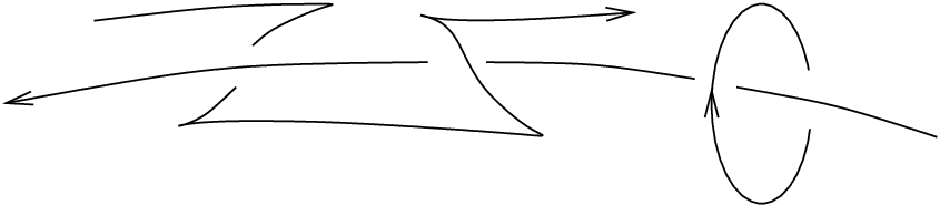
Then , so represents . For each of the meridional loops we add four cusps to the front projection (but leave its writhe unchanged), so
Since we have added as many up-cusps as down-cusps by introducing extra meridional loops, we have . Here we have used the well-known formulae for computing and from the front projection, cf. [7]. In the next section these formulae are stated for , but they hold equally in .
Case 3 (b2): , , and . Assume that is a Legendrian realisation of our –cable link with taking on the maximal possible value. By the now familiar argument involving Kanda’s theorem we may assume that sits on a convex torus standardly embedded in . Since equals the linking of with a push-off along , Kanda’s formula implies that the slope of must be . Moreover, it may be assumed that is in standard form, the number of Legendrian divides is two, and that is one of them (cf. the end of the proof of Lemma 4.8 in [9] and appeal to Giroux flexibility rel boundary [11], cf. [14, Thm. 3.4]).
Our first task is to show that the other classical invariants, i.e. , and , then determine up to Legendrian isotopy. Moreover, one has to determine the range of and, finally, to discuss the equivalence of Legendrian links , with equal invariants that destabilise to links with different invariants.
In order to deal with these issues, we need to recall an invariant of homology classes of curves on a convex torus in standard form, as defined in [9, p. 88]. Let be a globally non-zero section of , and a section of that is tangent to the Legendrian ruling curves and transverse to the Legendrian divides. (In [9], is chosen transverse to the ruling and tangent to the Legendrian divides, but up to homotopy this is the same as our choice.) For a closed, oriented curve on , define as the rotation of relative to along . This function has the following properties, which are not difficult to check (for the second one cf. the argument in the proof of Lemma 10 above).
- •
The function is well-defined and linear on homology classes.
- •
The function is invariant under isotopies of through convex tori in standard form.
- •
If is a Legendrian ruling curve or a Legendrian divide, then .
In particular, we have
The goal now is to show that actually determines and , and that this is the key to completing the classification. Since Etnyre and Honda may assume without loss of generality that , but we — unfortunately — may not, we have to make one last division into three subcases.
Case 3 (b2-i): , , , and . In this case, the arguments of [9] apply, and we only need to add a few details. Etnyre and Honda derive various properties of the function , notably the range of the values and . From there one concludes that the rotation number does indeed determine both and . Moreover, the possible values of (for being maximal) are shown to lie in
All these rotation numbers are realised by a Legendrian knot forming part of a cable link : in Figure 8 (bottom) of [9] one finds an explicit realisation of , to which a meridional loop can be added with and equal to one of the allowable values .
Lemma 11.
Let and be –cable links with . Then and are Legendrian isotopic if and only if .
Proof.
We split into a solid torus (with boundary , and in the complementary solid torus), a standard neighbourhood of , and a thickened torus with boundaries and ; similarly we define and .
The rotation number determines (which equals the rotation number of when the Legendrian ruling is made horizontal), and hence the contact structure on resp. by the classification of tight contact structures on solid tori [14, Prop. 4.23]. Thus, we have a contactomorphism .
Let be the corresponding function on homology classes of closed curves on . By slight abuse of notation, we regard and as classes both on and on , and we identify with . In the standard neighbourhood (as in Case 2), we may in fact take the vector field in the definition of to be equal to ; at any rate, extends as a nonzero section of over , coinciding with the tangent vector field to along that Legendrian curve. It follows that and .
The Legendrian rulings on and define a section of over , with and . Let be the corresponding relative Euler class. Then, up to sign convention,
and
It follows that and determine the relative Euler class of . The boundary slopes of are and . Thus, as in Case 2 we conclude that and are contactomorphic. As in the proof of Lemma 4, we find a contact isotopy that moves to itself and sends to . In that lemma, and the image of under the isotopy were Legendrian ruling curves and hence isotopic. Here, they are Legendrian divides, which are isotopic by [9, Lemma 3.17]. That lemma states that these divides can be realised as the intersection of with a pre-Lagrangian, i.e. linearly foliated torus with closed leaves (inside a small neighbourhood of ). Thus, the two Legendrian divides of are Legendrian isotopic via a family of leaves on the pre-Lagrangian torus. ∎
Remark.
The actual choice of Legendrian rulings on the two boundary tori is irrelevant for the computation of the relative Euler class, since all Legendrian rulings are homotopic to one another.
The following lemma is the direct analogue of Lemma 4.12 in [9], and the proof goes through essentially without any changes, except that once again we have to use the classification of tight contact structures on a thickened torus. By we denote the –fold positive resp. negative stabilisation of a Legendrian knot.
Lemma 12.
Let and be –cable links with . Write with and .
If , then and are Legendrian isotopic.
If , then and are Legendrian isotopic. ∎
From this lemma, the proof of Theorem 1 in Case 3 (b2-i) concludes as in Theorem 4.13 of [9]. The structure of the argument will become clearer in our discussion of the remaining cases, where we have to provide details, since [9] can no longer be invoked directly.
Case 3 (b2-ii): , (sic!), , and . Write with and . Thus the slope of lies in the interval . (Here the set-up with and maximal is as before.) By arguments as in the proof of Case 3 (a), we find a solid torus with convex boundary having two dividing curves of slope . Similarly, there is a solid torus containing in the interior, with convex boundary having two dividing curves of slope .
Let and be the functions on homology classes, as discussed in the preceding case, corresponding to the tori and , respectively. In order to apply the results of [9], we regard as the boundary of , with positive basis for given by meridian and longitude . In terms of this basis, we have . So the considerations of [9, pp. 88/89] for negative torus knots apply if we replace in their formulae by , respectively. This yields the following:
- (i)
or .
- (ii)
.
- (iii)
If , then .
- (iv)
If , then .
Here, however, the straightforward analogy with [9] ends, for the presence of now imposes additional restrictions on the allowable rotation numbers for . First we need the following lemma.
Lemma 13.
If , then . If , then .
Proof.
The fact that is implicit in [9, p. 92]. Here is the argument. Make the Legendrian ruling curves on and meridional, and let be a meridional annulus between the two tori, with Legendrian boundary . Denote the boundary curves of by and . With denoting either boundary curve and its push-off along , we have , and hence . So Kanda’s theorem allows us to assume that is convex.
The dividing curves on will intersect and in and points, respectively. As shown in [9, p. 92], there must be dividing curves running from to , and one dividing curve with both endpoints on , cutting off a disc-like region (a so-called boundary-parallel dividing curve). Otherwise there would be a boundary-parallel dividing curve for , and Etnyre and Honda show that this would give rise to an overtwisted disc.
By [14, Prop. 4.5], the relative Euler class of the thickened torus between and , when evaluated on , equals , i.e. the difference in Euler characteristics of the positive and negative regions into which the dividing curves partition . The dividing curves running from to give positive and negative disc-like regions; the boundary parallel arc adds one positive or negative disc-like region. It follows that , as claimed.
We now want to establish the sign in this equation. Consider the case that ; the case is completely analogous. Make the Legendrian ruling of by curves of slope , and let be an annulus between such a Legendrian ruling curve and a Legendrian divide (likewise of slope ) on . The linking of either boundary curve of with its push-off along equals , the maximal Thurston-Bennequin invariant of a –torus knot. Thus, Kanda’s formula and theorem once again imply that may be assumed to be convex. Let be the relative Euler class of the thickened torus between and . Then
The dividing curves of intersect on in two points. In a convex longitudinal disc with Legendrian boundary, therefore, there will be only one dividing curve, separating the disc into one positive and one negative region. Since may be computed by counting the difference between the number of positive and negative regions on a longitudinal disc (cf. [14, Prop. 4.23]), we have .
Arguing by contradiction, we now assume that . Then, together with equation (iii) before this lemma, we obtain
The dividing curves on do not intersect the boundary of ; the dividing curves on intersect the boundary of in
points. Thus, all (non-closed) dividing curves on have both endpoints on , and can be at most equal to (if there are positive disc-like regions and one negative annulus-like region on ) — unless there are closed dividing curves on .
Since our previous computation gave , such closed dividing curves would indeed have to exist. But this is impossible in a tight contact manifold by a criterion of Giroux, cf. [14, Thm. 3.5]. This contradiction proves the lemma. ∎
Corollary 14.
If , then
If , then
Proof.
This follows from by a straightforward computation, using the preceding lemma and equations (iii), (iv). ∎
Combined with the next lemma, this shows how the range of the rotation number is restricted by the value of (or vice versa). Observe that the equations and imply .
Lemma 15.
We have .
Proof.
Consider a convex meridional annulus, with Legendrian boundary curves, between the tori and . Analogous to the proof of Lemma 13, there must be dividing curves on this annulus running from one boundary component to the other, and dividing curves with both endpoints on . By the reasoning employed in that proof, the difference
can be at most equal to , the maximum being attained if all the extra dividing curves are boundary-parallel and separate off disc-like regions of the same sign. ∎
Lemma 13 and condition (ii) before that lemma (with replaced by ) yield:
- •
If , then
- •
If , then
This apparent dichotomy is only superficial. By some simple arithmetic, the condition on can be rewritten as
| (1) |
Not surprisingly, this is the same condition as in Case 3 (b2-i), with replaced by . However, it is no longer obvious how to add an unknot to Figure 8 (bottom) of [9] realising any combination of and , because now corresponds to a longitudinal curve in that figure. Indeed, the preceding lemmas give the restriction
| (2) |
with the choice of sign as in condition (1). Notice that by the parity condition
satisfied by any Legendrian knot in , cf. [5, Prop. 2.3.1], only every other value in the range allowed by condition (2) can actually be attained by .
We claim that all the rotation numbers allowed by conditions (1) and (2) are indeed realised by a Legendrian –cable link. By the observations above, Figure 8 (bottom) of [9] gives a Legendrian realisation of the –torus knot once we replace in that figure by .
Given this , we choose a solid torus as at the beginning of the discussion of the present Case 3 (b2-ii). With respect to the solid torus , the slope of is equal to . By the classification of tight contact structures on solid tori [14, Prop. 4.23], the contact structure on is unique up to isotopy, since a meridional disc of that torus is intersected only once by each of the two dividing curves, cf. the proof of Lemma 13. We may therefore identify with the solid torus in the standard model
Let be the Legendrian unknot in corresponding to the spine in that model, oriented so as to be isotopic to in our customary notation. Then and . By –fold stabilisation of , we obtain a Legendrian unknot topologically isotopic to , with and taking on any given value in the allowable range (subject to the parity condition mentioned above).
Lemma 11 is valid unchanged in the present case. Lemma 12 has to be replaced by the following, with the obvious changes in the proof.
Lemma 16.
Let and be –cable links with . Write with and .
If , then and are Legendrian isotopic.
If , then and are Legendrian isotopic. ∎
Now, again, the proof of Theorem 1 in Case 3 (b2-ii) concludes as in Theorem 4.13 of [9]. The argument goes as follows. Graph the possible pairs as dots in the plane, with labelled along a horizontal axis and along a vertical axis. Then these dots will form a ‘mountain range’, cf. Figure 9 of [9]. The peaks correspond to pairs with taking on the maximal value . By Lemma 11, there are unique Legendrian realisations of our cable link with having the classical invariants corresponding to such a peak (and a given allowable pair of classical invariants for the unknot ).
By condition (1), neighbouring peaks in that mountain range have distance or . Lemma 16 shows that the valley between any two such peaks also corresponds to a unique Legendrian realisation .
Since positive and negative stabilisations commute with each other, it is now elementary to see that any two Legendrian –cable links , with the same classical invariants can be destabilised to links , with invariants that are the same for both destabilisations and which allow a unique Legendrian realisation. This means that and are Legendrian isotopic, and so will be and .
Case 3 (b2-iii): , , and . The set-up with realising the maximal Thurston-Bennequin invariant is as described at the beginning of Case 3 (b2). Since now has integral slope , the considerations of the previous case give and
As seen in Case 3 (b2-i), for a standard neighbourhood of we have and . As in Lemma 15 we have
Thus, given , the conditions above give the allowable range of , which in turn determines via
All the rotation numbers allowed by these conditions can be realised by a Legendrian link as follows. Notice that the condition implies that is an unknot; this has a Legendrian realisation with and in the described range.
We now want to find a Legendrian unknot with and , where has to satisfy the Thurston-Bennequin inequality and the parity condition mod . Moreover, has to be in the class .
Set . The conditions above translate into , and together with the parity condition mod we get mod . We can therefore find unique non-negative integers satisfying
Let be the Legendrian push-off of (defined by a parallel copy of in the front projection picture as in the example at the end of case 3 (b1)), but with reversed orientation. Then , so may be regarded as a cable of representing the class . Now define as the stabilisation ; this does not change the topological picture.
We compute
and
Now we come to the proof of Theorem 1 in the present case. Since determines , the proof of Lemma 11 goes through as before. The analogue of Lemmas 12 and 16 is the following.
Lemma 17.
Let and be –cable links with . If , then and are Legendrian isotopic.
Proof.
Observe that the assumption implies that is not equal to the minimal possible value , hence .
In Section 4.4.5 of [14] it is explained how the classification of contact structures on a solid torus is achieved by decomposing a thickened torus into ‘positive’ and ‘negative layers’ of negative integer boundary slopes. The sign of these layers is exactly determined by the function . Moreover, positive and negative layers can be shuffled around. The fact that means that there must be at least one negative layer in , which we may take to be the outermost one. This implies that we can find a convex torus in with two dividing curves of slope and with .
Now consider an annulus between and of slope , with and equal to a Legendrian ruling curve. Both boundary curves satisfy the condition that allows us to assume that is convex: the Legendrian ruling curve must satisfy this condition with respect to the convex torus , and hence also with respect to ; the Legendrian divide actually has by Kanda’s formula.
The dividing curves of do not intersect the boundary component , and they intersect the boundary component on in
points. So there is one boundary-parallel dividing curve along . This implies that is a negative stabilisation of : the sign of the stabilisation follows from the condition and the fact that the Legendrian knots in question lie in the class .
Similarly, we find a convex torus in with two dividing curves of slope and
We then find an annulus with .
The proof of Theorem 1 now concludes exactly as in the previous two subcases.
5. Contact geometry of
In this section we discuss the classical invariants of Legendrian knots in the –jet space and prove Theorem 3. The definition of these invariants is based on Proposition 2.
Proof of Proposition 2.
Define a map by
with . This is a diffeomorphism of onto , where
A straightforward calculation yields
so is indeed a contactomorphism from to preserving (co-)orientations.
Remark.
The idea behind the definition of is the following: If we change coordinates on from to with
then , which exhibits an obvious Legendrian –fibration of over . Likewise, there is a Legendrian Hopf fibration of over . Take to be a fibre, and define sending fibres to fibres. In terms of the coordinates , the map is given by
It remains to check that . Recall that is the linking number of with a parallel copy obtained by pushing in the direction of a vector field along transverse to . A candidate for such a vector field is , so we may take
The linking number can be computed as the intersection number of Seifert surfaces and of and resp. in the –ball . For we may take the disc
for , the disc
These discs intersect at the origin only, and one checks that a positively oriented basis for the tangent space followed by a positive basis for is a negative basis for . ∎
By identifying with , we can visualise a Legendrian knot in its front projection to a strip in the –plane. The usual definition for the Thurston-Bennequin invariant of is
where the quantities on the right are computed from the front projection of . This is the signed number of crossing changes required to ‘unlink’ from its push-off in the –direction (i.e. transverse to ), that is, the number of crossing changes that will allow one to separate the two knots in .
The images of the curves , , under the contactomorphism are Hopf fibres, any two of which have linking number . This accounts for the correction term between and .
Regarding the rotation number, we observe the following. The contact structure admits the global sections and . For an oriented Legendrian knot , the rotation number counts the rotations of a positive tangent vector to relative to this ordered basis of sections as we go once around . Similarly, in one counts rotations relative to a trivialisation and orientation of given by the vector fields
where these vector fields are written in terms of the basis . We compute
which is homotopic through nonvanishing sections of to the vector field . This proves that . The same considerations as for the standard contact structure on (defined likewise by , now with ) apply to show that in the front projection to the –plane we have
with the number of cusps oriented upwards or downwards, respectively.
Proof of Theorem 3.
Let and be two oriented Legendrian torus knots in which have the same oriented knot type and classical invariants. With denoting the contactomorphism defined in the proof of Proposition 2, we have the Legendrian cable links and in . The formulae relating the classical invariants in and imply that and have the same invariants and are therefore isotopic by Theorem 1. Notice that because of , the case discussed after the proof of Lemma 5, where we might have had to reverse the roles of and , does not occur.
The proof of Theorem 1 does not, however, guarantee the existence of an isotopy fixing . Instead, we may argue as follows. What the proof does give is a contactomorphism of sending to and equal to the identity map in a neighbourhood of . This translates into a contactomorphism of sending to , equal to the identity map outside a compact set.
If we change coordinates on from to with
then . This identifies as the space of cooriented contact elements of .
A contactomorphism of that space, fixed outside a compact set, may be regarded as a contactomorphism of the space of contact elements of the closed –disc , fixed near the boundary . According to [13, Thm. 1], the isotopy classification of such contactomorphisms coincides with the isotopy classification of diffeomorphisms of , fixed near the boundary.
By a beautiful argument of Smale [19], any diffeomorphism of fixed near the boundary is isotopic to the identity map. ∎
6. Transverse knots and links
The argument of [9, Thm. 2.10] concerning the classification of transverse knots in a contact manifold (i.e. knots everywhere transverse to the contact structure) via that of Legendrian knots carries over without changes and yields the following corollary to Theorems 1 and 3. Notice that transverse knots and links carry a natural orientation making them positively transverse to the given (cooriented) contact structure.
Corollary 18.
Transverse cable links in are classified up to transverse isotopy by their oriented link type and the self-linking numbers of the two components.
Transverse torus knots in are classified up to transverse isotopy by their oriented knot type and self-linking number. ∎
Acknowledgements.
F. D. is partially supported by grant no. 10201003 of the National Natural Science Foundation of China. H. G. is partially supported by grant no. GE 1245/1-1 of the Deutsche Forschungsgemeinschaft within the framework of the Schwerpunktprogramm 1154 “Globale Differentialgeometrie”. Most of this research was carried out during a visit by F. D. to the Mathematical Institute of the Universität zu Köln.
References
- [1] G. Burde and H. Zieschang, Knots, de Gruyter Stud. Math. 5 (Walter de Gruyter & Co., Berlin, 1985).
- [2] Yu. Chekanov, Differential algebra of Legendrian links, Invent. Math. 150 (2002), 441–483.
- [3] F. Ding and H. Geiges, A Legendrian surgery presentation of contact –manifolds, Math. Proc. Cambridge Philos. Soc. 136 (2004), 583–598.
- [4] Ya. Eliashberg, Contact –manifolds twenty years since J. Martinet’s work, Ann. Inst. Fourier (Grenoble) 42 (1992), 165–192.
- [5] Ya. Eliashberg, Legendrian and transversal knots in tight contact –manifolds, in Topological Methods in Modern Mathematics (Stony Brook, NY, 1991) (Publish or Perish, Houston, 1993), pp. 171–193.
- [6] Ya. Eliashberg and M. Fraser, Classification of topologically trivial Legendrian knots, in Geometry, Topology, and Dynamics (Montréal, 1995), CRM Proc. Lecture Notes 15 (American Mathematical Society, Providence, 1998), pp. 17–51.
- [7] J. B. Etnyre, Introductory lectures on contact geometry, in Topology and Geometry of Manifolds (Athens, GA, 2001), Proc. Sympos. Pure Math. 71 (American Mathematical Society, Providence, 2003), pp. 81–107.
- [8] J. B. Etnyre, Legendrian and transversal knots, in Handbook of Knot Theory (North-Holland, Amsterdam), to appear.
- [9] J. B. Etnyre and K. Honda, Knots and contact geometry I: Torus knots and the figure eight knot, J. Symplectic Geom. 1 (2001), 63–120.
- [10] H. Geiges, Contact geometry, in Handbook of Differential Geometry, vol. 2 (North-Holland, Amsterdam), to appear.
- [11] E. Giroux, Convexité en topologie de contact, Comment. Math. Helv. 66 (1991), 637–677.
- [12] E. Giroux, Structures de contact en dimension trois et bifurcations des feuilletages de surfaces, Invent. Math. 141 (2000), 615–689.
- [13] E. Giroux, Sur les transformations de contact au-dessus des surfaces, in Essays on Geometry and Related Topics, eds. É. Ghys et al., vol. 2, Monogr. Enseign. Math. 38 (Genève, 2001), pp. 329–350.
- [14] K. Honda, On the classification of tight contact structures I, Geom. Topol. 4 (2000), 309–368; erratum: Factoring nonrotative layers, Geom. Topol. 5 (2001), 925–938.
- [15] Y. Kanda, On the Thurston-Bennequin invariant of Legendrian knots and nonexactness of Bennequin’s inequality, Invent. Math. 133 (1998), 227–242.
- [16] J. Milnor, Singular Points of Complex Hypersurfaces, Annals of Math. Studies 61 (Princeton University Press, 1968).
- [17] L. Ng, Computable Legendrian invariants, Topology 42 (2003), 55–82.
- [18] L. Ng and L. Traynor, Legendrian solid-torus links, J. Symplectic Geom., to appear.
- [19] S. Smale, Diffeomorphisms of the –sphere, Proc. Amer. Math. Soc. 10 (1959), 621–626.