Complements of tori and Klein bottles in the4-sphere that have hyperbolic structure

Let $\mathbf{H}^{n}$ be the $n$-dimensional hyperbolic space and let $G$ be a discrete subgroup of $\Isom\mathbf{H}^{n}$, the isometries of $\mathbf{H}^{n}$. If $G$ is torsion-free, then $M=\mathbf{H}^{n}/G$ is a hyperbolic manifold of dimension $n$. A hyperbolic manifold of interest in this paper is also complete, noncompact and has finite volume and the term “hyperbolic manifold” will be understood to include those additional properties. Such a manifold $M$ is the interior of a compact manifold with boundary $\overline{M}$. Every boundary component $E$ of $\overline{M}$ is a compact flat (Euclidean) manifold, i.e. a manifold of the form $\mathbf{R}^{n-1}/K$, where $K$ is a discrete subgroup of $\Isom\mathbf{R}^{n-1}$, the isometries of $\mathbf{R}^{n-1}$. For simplicity, we sometimes inaccurately call $E$ a boundary component of $M$ (rather than $\overline{M}$, whose boundary component it really is).

When $n=3$, $M$ is the interior of a compact 3-manifold $\overline{M}$ whose boundary consists of tori and Klein bottles. When all the boundary components are tori, $M$ may be diffeomorphic to $S^{3}$ with several closed solid tori removed, which in turn is diffeomorphic to $S^{3}-A$, where $A$ is the link consisting of the core circles of the solid tori. Indeed, it is a well known fact that many hyperbolic 3-manifolds are link complements in $S^{3}$.

The first example of a generalization of this situation to dimension 4 was given by Ivanšić [6], where it was shown that $\widetilde{M}_{1011}$, the orientable double cover of one of the 1049 nonorientable hyperbolic 4-manifolds that Ratcliffe and Tschantz constructed [9], is a complement of 5 tori in $S^{4}$. Finite covers of $\widetilde{M}_{1011}$ were also shown to be complements of a collection of tori in a simply-connected 4-manifold with even Euler characteristic.

In this paper, we find 11 additional examples of hyperbolic 4-manifolds that are complements in $S^{4}$ of a set of tori or a combination of tori and Klein bottles. The list of examples is in Theorem 4.4. Like $\widetilde{M}_{1011}$, all of them are orientable double covers of some of Ratcliffe and Tschantz’s nonorientable manifolds. Proving that those manifolds are complements in $S^{4}$ is typically trickier than in [6], since the many symmetries of $M_{1011}$ enabled an easier computation.

By taking finite covers of some of the link complements we also find additional examples of hyperbolic 4-manifolds that are complements of a collection of tori and Klein bottles in a simply-connected 4-manifold with even Euler characteristic. Example 4.10 displays 8 different families of examples, illustrating the richness of such objects, many more of which likely exist.

Manifolds $\widetilde{M}_{1091}$ and $\widetilde{M}_{1011}$ were used by Ratcliffe and Tschantz [10] to construct the first examples (infinitely many) of aspherical homology 4-spheres. Three other examples in this paper can be used for the same purpose, see Example 4.11.

When looking for examples of link complements in $S^{4}$ among the orientable double covers of the 1049 nonorientable manifolds, the main difficulty is to reduce the number of potential examples with which to experiment. We use a homological and a group-theoretical criterion (see §4) to rule out all except 49 manifolds from having the desired property. Then we show that some of the remaining 49 manifolds have orientable double covers that are complements of tori and Klein bottles in the 4-sphere. Essentially, we use group presentations to show that the manifold $N$ resulting from closing up the boundary components of the double covers is simply-connected. This, along with the fact that the Euler characteristic $\chi(N)$ is 2, guarantees that $N$ is homeomorphic to $S^{4}$.

Ratcliffe and Tschantz constructed their manifolds by side-pairings of a hyperbolic noncompact right-angled 24-sided polyhedron, making computations with them laborious, especially if they have to be done repeatedly. The two criteria were checked using a computer, but we emphasize that the results of this paper do not depend on a computer calculation, since it is verified by hand that some of the “promising” examples indeed have a double cover that is a complement in the 4-sphere.

Let $M$ be hyperbolic $n$-manifold. We say that $M$ is a (codimension-2) complement in $N$ if $M=N-A$, where $N$ is a closed $n$-manifold and $A$ is a closed $(n-2)$-submanifold of $N$ that has a tubular neighborhood in $N$ and has as many components as $\partial\overline{M}$. Then every component $E$ of $\partial\overline{M}$, being the boundary of a tubular neighborhood, must be an $S^{1}$-bundle over a component of $A$. The $(n-1)$-manifold $E$ is flat. The following theorem (see [5] or [1] Theorem 6.40) summarizes when a flat manifold is an $S^{1}$-bundle and, when it is, what its $S^{1}$-fibers are.

We say that a translation $t$ is normal in $E$ if $\left<t\right>$ is a normal subgroup, we say it is primitive in $E$ if it is not a power of any other element of $K$.

By Theorem 2.1, if $M$ is a hyperbolic 4-manifold that is a complement in $N$, it must be a complement of flat 2-manifolds, that is, tori and Klein bottles. We are interested in the case when $N=S^{4}$. When $M=N-A$, an immediate consequence of the fact that components of $A$ are flat is that $\chi(M)=\chi(N)$, so examples of complements in $S^{4}$ must be searched for among manifolds with $\chi(M)=2$. Nonorientable examples of Ratcliffe and Tschantz are very suitable for this purpose, since their Euler characteristic is 1: passing to the orientable double cover will give us the required Euler characteristic.

Once we have found a hyperbolic manifold $M$ all of whose boundary components are $S^{1}$-bundles, $M=N-A$. To show that $N$ is a topological $S^{4}$, it suffices to show that $\pi_{1}N=1$ and $\chi(N)=2$ (see [3] or [2]). The following application of van Kampen’s theorem shows how to compute $\pi_{1}N$ from $\pi_{1}M$; details are in [6].

Hyperbolic manifolds $M$ of interest in this paper are given by side-pairings of a hyperbolic finite-volume noncompact polyhedron $Q$. Side-pairings determine sets of points on the polyhedron, called cycles, that are identified in the manifold. Boundary components of $\overline{M}$ correspond to cycles of ideal vertices of $Q$. If $[v_{i}]$ is the cycle of an ideal vertex corresponding to $E_{i}$, then $\stab v_{i}$ is isomorphic to $\pi_{1}E_{i}$, making the inclusion $\pi_{1}E_{i}\to\pi_{1}M$ injective. Elements of $\pi_{1}E_{i}$ are parabolic isometries, thus, they preserve horospheres centered at $v_{i}$ and act like Euclidean isometries on them.

Let $\Gamma$ be a discrete subgroup of $\Isom\mathbf{H}^{n}$ with fundamental polyhedron $P$. Then $\Gamma$ is generated by side-pairings of $P$, isometries that send a side of $P$ to another side of $P$. If $s$ is an isometry sending side $S$ of $P$ to $S^{\prime}$, then, if we start moving from $P$ and pass through $S$, we wind up in $s^{-1}P$. Similarly, if we take a path $P$ to $\gamma P$ that passes through interiors of translates of sides $S_{1},\dots,S_{m}$ whose side-pairings are $s_{1},\dots,s_{k}$, then $\gamma=s_{1}^{-1}\dots s_{m}^{-1}$. Furthermore, if $G$ is a finite-index subgroup of $\Gamma$ with transversal $X$ (that is, a set of right-coset representatives, so $\Gamma=\cup_{x\in X}Gx$), then the fundamental polyhedron of $G$ is $Q=\cup_{x\in X}xP$, where elements of $X$ can be chosen so that $Q$ is connected.

The fundamental groups $G$ of Ratcliffe and Tschantz’s manifolds are all minimal index torsion-free subgroups of a certain reflection group $\Gamma$, which is generated by reflections in a 10-sided right-angled polyhedron $P$. The side-pairings generating $\Gamma$ are, of course, reflections in the sides of $P$. Every subgroup $G$ corresponding to a Ratcliffe-Tschantz manifold has the same transversal in $\Gamma$, a finite group $K$ isomorphic to $\mathbf{Z}_{2}^{4}$ and generated by reflections in the four coordinate planes in the ball model of $\mathbf{H}^{4}$. The fundamental polyhedron of $G$ is $Q=KP$, a 24-sided regular right-angled hyperbolic polyhedron that we call the 24-cell. Let $f$ be a side-pairing of $Q$ that sends side $R$ to side $R^{\prime}$. As was shown in [9] and [6], $f$ has to have form $f=kr=r^{\prime}k$, where $k\in K$ is an element such that $k(R)=R^{\prime}$, and $r$, $r^{\prime}$ are reflections in $R$, $R^{\prime}$, respectively. We will call $k$ the $K$-part of $f$. Thus, it is enough to specify elements $k\in K$ in order to define a side-pairing of $Q$.

As is clear from Theorem 2.1 and Proposition 2.2, we will need the ability to recognize when a composite of side-pairings is a translation. The following proposition, proved in [6], will be used for that purpose:

In this paper we work with presentations of groups and their subgroups. If a group $G$ is given by presentation $\left<Y\,|\,R\right>$, and $H$ is a finite-index subgroup of $G$ with Schreier transversal $X$ (i.e. $G=\cup_{x\in X}Hx$ and every initial segment of an element $x\in X$ is also an element of $X$), then the presentation of $H$ can be derived from the presentation of $G$. Let $g\mapsto\overline{g}$ be the map $G\to X$ sending $g$ to its coset representative, that is $Hg=H\overline{g}$, and let $\gamma:G\to H$ be the map $\gamma(g)=g{\overline{g}}^{-1}$.

Working in the ball model of $\mathbf{H}^{4}$, let $S_{****}$ be one of the 24 spheres of radius 1 centered at a point in $\mathbf{R}^{4}$ whose coordinates have two zeroes and two $\pm 1$’s. The string $*$$*$$*$$*$ consists of symbols $+$,$-$,0 and identifes the sphere by its center. For example, $S_{+0-0}$ is the sphere centered at $(1,0,-1,0)$. These spheres are orthogonal to $\partial\mathbf{H}^{4}$, hence they determine hyperplanes in $\mathbf{H}^{4}$. The 24-sided polyhedron $Q$ is defined to be the intersection of the half-spaces corresponding to those hyperplanes that contain the origin. The side of $Q$ lying on the sphere $S_{****}$ is also denoted by $S_{****}$. All the dihedral angles of $Q$ are $\pi/2$ and its 24 ideal vertices are $v_{\pm 000}=(\pm 1,0,0,0)$, $v_{0\pm 00}=(0,\pm 1,0,0)$, $v_{00\pm 0}=(0,0,\pm 1,0)$, $v_{000\pm}=(0,0,0,\pm 1)$ and $v_{\pm\pm\pm\pm}=(\pm 1/2,\pm 1/2,\pm 1/2,\pm 1/2)$. The polyhedron $Q$ has no real vertices.

Note that two sides intersect if and only if their identifying strings have equal nonzero entries in one position and the positions of the remaining nonzero entries are different. Two sides touch at $\partial\mathbf{H}^{4}$ when they have equal nonzero entries in one position and opposite nonzero entries in another position, or if the positions where they have nonzero entries are complementary. Furthermore, an ideal vertex is on a side if its Euclidean distance from the center of the sphere defining the side is 1. In the case of vertices whose label has one nonzero entry, a vertex is on a side if and only if the side has an equal nonzero entry in the same position as the vertex; in the case of vertices $v_{\pm\pm\pm\pm}$, a vertex is on a side if and only if the nonzero entries in the label of the side coincide with the entries in the label of the vertex in the same position. For example, $S_{0-+0}$ and $S_{+-00}$ intersect, $S_{0-+0}$ and $S_{0+0+}$ are disjoint, the side $S_{0+0-}$ has six ideal vertices $v_{0+00}$, $v_{000-}$, $v_{\pm+\pm-}$; $S_{0-+0}$ and $S_{0--0}$ touch at $v_{0-00}$, and $S_{0-+0}$ and $S_{-00-}$ touch at $v_{--+-}$.

As mentioned in §2, every Ratcliffe-Tschantz example has side-pairing isometries of form $rk$, where $k\in\mathbf{Z}_{2}^{4}$ is a composite of reflections in the coordinate planes $x_{1}=0,\dots,x_{4}=0$. The label $\pm$$\pm$$\pm$$\pm$ identifies an element of $K$, for example, $k_{+--+}$ is the composite of reflections in $x_{2}$ and $x_{3}$. Ratcliffe and Tschantz have found in [9] that all sides whose labels have nonzero entries in the same two positions must have the same $K$-part for their side-pairing.

Side-pairing labeling convention Group letters $a,\dots,l$ and the sides of $Q$ as follows:

The two letters in each group denote the side-pairings of the four sides from the group. The first letter always pairs the side labeled $++$, and the second letter pairs the side whose label is the next unused one, where the symbols $\pm\pm$ have been ordered in the dictionary order: $++$, $+-$, $-+$, $--$.

The encoding of the side-pairing transformation is done like in [9]. A string of six characters from $\{1,\dots,9,A,\dots,F\}$, one for each group above, encodes the $K$-part of each side-pairing. Each character stands for a hexadecimal number, which is turned into binary form and the order of digits is reversed. Converting every 0 into a plus and every 1 into a minus obtains the label of $k$. For example, $1$ stands for $k_{-+++}$; $C=12$ stands for $k_{++--}$. (See Example 4.6.)

The presentation of a group $G$ generated by side-pairings of a polyhedron is obtained by applying Poincaré’s polyhedron theorem ([8] Theorem 11.2.2). Finding presentations of the groups and identifying usable translations in parabolic groups is crucial to our proof of Theorem 4.4. An efficient method for these two tasks is essential if one is to deal with a dozen examples, so we elaborate on it.

Let $C$ be a small enough horosphere centered at $v_{++++}$ that intersects only the sides of $Q$ that contain $v_{++++}$. Then $Q_{C}=C\cap Q$ is a cube with opposing sides $S_{++00}$ and $S_{00++}$, $S_{+0+0}$ and $S_{0+0+}$, $S_{0++0}$ and $S_{+00+}$ (see Figure 1). The tiling of $\mathbf{H}^{4}$ by translates of $Q$ intersected with $C$ gives a tiling of $C$ by cubes, one of which is $Q_{C}$.

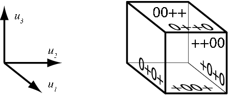
We use the term ridge to denote a codimension-2 face of a polyhedron, while an edge is a 1-face. Every edge of the cube $Q_{C}$ represents a ridge of $Q$. Circling around the edge once gives a cycle relation for the presentation in Poincaré’s theorem. To easily determine which sides we pass through, use Figure 2. The left column depicts the intersections of the tiling of $C$ with the three planes that pass through the center of $Q_{C}$ and are parallel to its sides. The side-pairings in that figure are the ones for manifold $M_{56}$ from Example 4.6.

Let $s$ be the side-pairing sending $S$ to $S^{\prime}$, $r_{S}$ the reflection in $S$ and let $k_{S}$ be the $K$-part of $s$. Consider a ridge $U\cap S$, where $U$ is another side of $Q$. The ridge $U\cap S$ is sent via $s$ to a ridge $V\cap S^{\prime}$, where $V$ is another side of $Q$. Now $V\cap S^{\prime}=k_{S}r_{S}(U\cap S)=k_{S}(U\cap S)=k_{S}(U)\cap S^{\prime}$ so we conclude $V=k_{S}(U)$. Therefore, adjacent to $Q$ on the other side of $S$ is $s^{-1}Q$, whose sides $s^{-1}V$ and $s^{-1}S^{\prime}$ meet at ridge $U\cap S=s^{-1}(V\cap S^{\prime})$.

The observation $V=k_{S}(U)$ allows us to easily find the labelings on all the struts in the diagrams in the left column of Figure 2 (labelings inside the square come from $Q_{C}$). For example, consider the sides around the vertex labeled 1 in the topmost diagram. The bottom left strut is the translate of the side $k_{S_{+00+}}(S_{0+0+})=k_{-++-}(S_{0+0+})=S_{0+0-}$, whose side-pairing is $j$. The left bottom strut is the translate of $k_{S_{0+0+}}(S_{+00+})=k_{--++}(S_{+00+})=S_{-00+}$, whose side-pairing is $h^{-1}$.

Cycle relations are words obtained circling an edge of $Q_{C}$ and successively adding the side-pairings at the end of the word. Care must be taken to add $s^{-1}$ at the end of the word whenever we exit through a side labeled $s$ and to add $s$ whenever we enter into a side labeled $s$. Going in the direction of the arrow around vertex 1 we exit through $g$ and $j$ and then enter into $h^{-1}$ and $i$, so the cycle relation is $g^{-1}j^{-1}h^{-1}i=1$.

We thus obtain 12 relations for $G$ from the first column of Figure 2. Because $Q$ has 96 ridges that fall into 24 ridge cycles, each corresponding to a relation, 12 further relations are needed. They are found by going around other edges in the tiling of $C$. If we reflect the three planes we used for sections of $Q_{C}$ in the sides of $Q_{C}$ parallel to them, we get new sections of the tiling represented by diagrams in the middle and right columns of Figure 2. The fact $V=k_{S}(U)$ from above is now used to see that the labelings on the new diagrams are obtained by applying $k_{S}$ to every label in the original diagram, where $S$ is the side used to reflect the section plane.

The middle and right columns do not include struts because cycle relations follow from only the labels on the square part and the cycle relations for the left column. If $A=\{S_{1},kS_{1},S_{2},kS_{2}\}$ is the set of four sides whose labels all have the same nonzero positions, and are hence paired by the same element $k\in K$, we note that any element $k^{\prime}\in K$ acts on $A$ and, due to commutativity of $K$, preserves or interchanges the subsets of $A$ containing paired sides. Along with the fact that $k^{\prime 2}=1$ for every $k^{\prime}\in K$ this means that action of $k^{\prime}$ on $A$ can be inferred just from knowing $k^{\prime}S_{1}$. For example, in the third row in Fig. 1, we see that by applying $k_{S_{0++0}}$ to the sides labeled $i$ and $a$ we get sides labeled $j$ and $a^{-1}$. We infer that applying $k_{S_{0++0}}$ to sides labeled $j$ and $b$ gives sides labeled $i$ and $b^{-1}$. Thus, the cycle relation for vertex 2 in the new diagram is the cycle relation $i^{-1}b^{-1}ia$ for vertex 2 in the old diagram with letters replaced in the above pattern, obtaining $j^{-1}bja^{-1}$. Now, if a cycle relation coming from the new diagram is the inverse, a cyclic permutation or a combination of the two of a corresponding cycle relation in the old diagram, we have found the same ridge cycle, and have to reflect the section plane in the other side of the cube $Q_{C}$.

We argue that the nine diagrams thus obtained will contain all the cycle relations (multiple times, in fact). Note that in $Q$ every ridge is an ideal triangle, two of whose ideal vertices are of type $v_{\pm\pm\pm\pm}$. For example, the ridge $R=S_{0+0+}\cap S_{0++0}$ is an ideal triangle with vertices $v_{0+00}$, $v_{++++}$ and $v_{-+++}$ and edges $E_{1}=S_{0+0+}\cap S_{0++0}\cap S_{00++}$, $E_{2}=S_{0+0+}\cap S_{0++0}\cap S_{++00}$, and $E_{3}=S_{0+0+}\cap S_{0++0}\cap S_{-+00}$. The intersection of translates of edges of $Q$ with $C$ are the vertices in the tiling of $C$. An edge of the cube $Q_{C}$ is an arc in the ideal triangle going from one edge of the triangle to another. Because elements of $K$ do not change the nonzero positions in the labeling of sides, only $E_{2}$ and $E_{3}$ might be in the same cycle of edges. Thus, in the manifold $\mathbf{H}^{4}/G$ the ideal triangle might only have its edges $E_{2}$ and $E_{3}$ identified, since no points on $E_{1}$ are identified. If ridge $R$ and the ridge represented by reflection of $R\cap C$ in the side $S_{00++}$ of $Q_{C}$ were in the same cycle, the segment consisting of $R\cap C$ and its reflection would project to a smooth curve in the ideal triangle that crosses $E_{1}$ twice, which is impossible. Since in $Q$ there are only 8 ridges of type $S_{0\pm 0\pm}\cap S_{0\pm\pm 0}$ we conclude that every one of them is either in the cycle of $R$, or the cycle of the ridge represented by the reflection of $C\cap R$ in $S_{00++}$. Reasoning similarly for all the other ridge cycles we see that the opportunity for cycle relation repetitions occurs only for ridges represented by vertices labeled 2 and 3 in the middle column. Often there are no repetitions: in Example 4.6 we needed three section planes only in the first row.

Now we describe how to identify and choose suitable translations in parabolic subgroups. Let $G_{v}$ be the parabolic group that is the stabilizer of an ideal vertex $v$ of $Q$, and let $C$ be a horosphere centered at $v$. The intersection $Q_{C}=Q\cap C$ is always a Euclidean cube. Position a coordinate system with origin in the center of $Q_{C}$ and axes perpendicular to its sides, and consider the tiling of $C$ by translates of $Q_{C}$. To simplify language, we identify a cube $gQ_{C}$ and the element $g$. According to Proposition 2.3, by considering a path from $Q_{C}$ to $gQ_{C}$ that passes only through sides of cubes (e.g. a path that is piecewise parallel to the coordinate axes), we may write $g=(r_{m}\dots r_{1})(k_{1}^{-1}\dots k_{m}^{-1})$. Since $r_{m}\dots r_{1}$ preserves $v$, $g\in G_{v}$ if and only if $k_{1}^{-1}\dots k_{m}^{-1}v=v$.

Let $v=v_{+000}$, $v_{0+00}$, $v_{00+0}$ or $v_{000+}$. The coordinate axes perpendicular to sides of $Q_{C}$ may be identified with coordinate axes $x_{1}$, $x_{2}$, $x_{3}$ and $x_{4}$, in the arrangement suggested by Figure 3. The 4-symbol labels on the axes indicate which side we pass through if we move from the center of $Q_{C}$ in the direction of the arrow. Parallel sides of each $Q_{C}$ have same nonzero positions but differ in sign in positions other than the nonzero position of the vertex label (a side and a vertex have the same symbol in the nonzero position of the vertex label when the vertex is on the side). Moving two steps in the directions of the axes produces translations since $k_{1}=k_{2}$ in every case. Let $T_{v}$ be the subgroup of $G_{v}$ generated by those three translations and let $TG_{v}$ be the translation subgroup of $G_{v}$. For our purposes we look for translations only in $8Q_{C}$, the $2\times 2\times 2$ block of cubes that is the fundamental polyhedron for $T_{v}$. A Euclidean transformation $Ax+a$ is a translation if and only if its rotational part $A$ is the identity. We get the rotational part of $r_{m}\dots r_{1}k_{1}^{-1}\dots k_{m}^{-1}$ by replacing $r_{i}$ by an element $k_{r_{i}}$ that represents the reflection in the coordinate plane parallel to the reflection plane of $r_{i}$ and computing the product. Note that it is enough to find the rotational parts of the three cubes adjacent to $Q_{C}$ in the direction of the three axes. Any other rotational part is obtained by multiplying those three: every time we move by one step in the direction of an axis, we multiply by the rotational part of one of the three cubes that corresponds to that axis. The dots in Figure 3 represent centers of cubes comprising $8Q_{C}$; the dot is filled if it corresponds to an element preserving $v$. Labels on the dots give the rotational part of the group element corresponding to the dot. The three zero positions in the vertex label give the rotational part of the transformation, while the nonzero position tells whether the transformation preserves $v$. For example, in the topmost diagram in Figure 3 the label $+$$+$$-$$+$ on a vertex reveals an element that preserves $v$ whose rotational part is a reflection in the $x_{3}$-plane. The label $-$$-$$+$$+$ reveals that the corresponding element does not preserve $v$. Arrows in the middle column indicate translations found in $8Q_{C}$, they correspond to dots labeled $+$$+$$+$$+$. The right column of the diagram computes the group elements corresponding to the dots of interest. This is done by considering which translates of sides we pass through as we go from $Q_{C}$ to the dot.

Let $v=v_{++++}$, then $Q_{C}$ is the cube from Figure 1. Here the condition $k_{1}^{-1}\dots k_{m}^{-1}v=v$ becomes $k_{1}^{-1}\dots k_{m}^{-1}=1$, since $K$ acts freely on the set of vertices $v_{\pm\pm\pm\pm}$. Moving four steps in the directions of the three axes produces translations because $k_{1}=k_{3}$, $k_{2}=k_{4}$ and $r_{1}\dots r_{4}$ is a composite of reflections in four parallel planes. Let $T_{v}$ be the subgroup of $G_{v}$ generated by those three translations and $TG_{v}$ be the translation subgroup of $G_{v}$. For our purposes, we look for translations in $64Q_{C}$, the $4\times 4\times 4$ block of cubes that is the fundamental polyhedron for $T_{v}$. It is clear that we get a translation if and only if we move an even number of steps in the direction of each axis, and have $k_{1}^{-1}\dots k_{m}^{-1}=1$. Therefore, we have to check $k_{1}^{-1}\dots k_{m}^{-1}=1$ for the 7 cubes obtained by moving $Q_{C}$ by a combination of two units in every direction. The dots in Figure 4 depict the centers of some cubes in $64Q_{C}$, and the ones at the vertices of the cube are the interesting ones. Labels indicate the products of the $K$-parts, so a $+$$+$$+$$+$ label means the dot corresponds to a translation. At right we compute the group elements corresponding to the dots of interest. One of the translations is omitted, since it is the sum of the other two in the diagram.

In this section we show that 12 nonorientable Ratcliffe-Tschantz manifolds have orientable double covers that are complements of tori and Klein bottles in $S^{4}$. First of all, we need criteria that rule out a manifold from having this property. The first criterion is:

The other criterion was developed in [6] and exploits a homomorphism that exists for every group $G$ of a Ratcliffe-Tschantz manifold. It is defined by $\phi:G\to\mathbf{Z}_{2}^{6}$, $a,b\mapsto e_{1}$, $c,d\mapsto e_{2},\dots,k,l\mapsto e_{6}$, where $e_{i}$ is a canonical generator of $\mathbf{Z}_{2}^{6}$.

Using a computer to test the 1149 nonorientable Ratcliffe-Tschantz manifolds for both criteria, we found that only 49 remained eligible to have double-cover complements in $S^{4}$, namely, manifolds numbered

If the double cover of any of these manifolds is a complement in $S^{4}$, the potential link structure is visible from its homology by Proposition 4.1. The computer calculation showed that only twelve different link structures are possible. We then proceeded to prove (manually) that for each of those link structures there is at least one manifold from the above list whose orientable double cover is the complement of such a link in $S^{4}$. Those manifolds are listed in Theorem 4.4. Most likely, other manifolds from the list above have the same property, but it is not easy to ascertain that we will be getting examples different from the ones in Theorem 4.4, since orientable double covers of nonisometric manifolds may be isometric.

Let $G$ be any group, $H$ a normal subgroup of $G$ and let $\left<\left<A\right>\right>_{H}$ be the normal closure of a set $A\subset H$ in $H$. If $G$ is the biggest group under consideration, $\left<\left<A\right>\right>$ or $\left<\left<A\right>\right>_{G}$ will denote the normal closure of $A$ in $G$. Clearly, $\left<\left<A\right>\right>_{H}$ is the set of all elements of the form $\prod h_{i}a_{i}h_{i}^{-1}$, where $h_{i}\in H$, $a_{i}\in A\cup A^{-1}$. If $X$ is a transversal of $H$ in $G$ it is easy to see that for a set $A\subset H$, $\left<\left<A\right>\right>_{G}=\left<\left<xAx^{-1},\ x\in X\right>\right>_{H}$. Note that $\left<\left<A\right>\right>_{G}$ is a subgroup of $H$, since $H$ is normal in $G$.

While $\left<\left<A\right>\right>_{H}\subseteq\left<\left<A\right>\right>_{G}$, in general, $\left<\left<A\right>\right>_{H}\neq\left<\left<A\right>\right>_{G}$. For example, if $H=\left<a\right>*\left<b\right>$, $G=H\rtimes\mathbf{Z}_{2}$, where $\mathbf{Z}_{2}$ acts on $H$ by swapping the generators $a$ and $b$, then clearly $\left<\left<a\right>\right>_{G}=H$, while $\left<\left<a\right>\right>_{H}$ is a subgroup of $H$ with infinite index.

The following proposition will prove useful.

References

- [1] B N Apanasov, Conformal geometry of discrete groups and manifolds, de Gruyter Expositions in Mathematics 32, Walter de Gruyter & Co., Berlin (2000) \MR1800993
- [2] M H Freedman, F Quinn, Topology of 4-manifolds, Princeton Mathematical Series 39, Princeton University Press, Princeton, NJ (1990) \MR1201584
- [3] R E Gompf, A I Stipsicz, -manifolds and Kirby calculus, Graduate Studies in Mathematics 20, American Mathematical Society, Providence, RI (1999) \MR1707327
- [4] W Hantzsche, H Wendt, Dreidimensionale euklidische Raumformen, Math. Ann. 110 (1935) 593–611
- [5] D Ivanšić, Embeddability of noncompact hyperbolic manifolds as complements of codimension-1 and -2 submanifolds, Topology Appl. 120 (2002) 211–236 \MR1895493
- [6] D Ivanšić, Hyperbolic structure on a complement of tori in the 4-sphere, Adv. Geom. 4 (2004) 119–139
- [7] R C Lyndon, P E Schupp, Combinatorial group theory, Classics in Mathematics, Springer-Verlag, Berlin (2001) \MR1812024
- [8] J G Ratcliffe, Foundations of hyperbolic manifolds, Graduate Texts in Mathematics 149, Springer-Verlag, New York (1994) \MR1299730
- [9] J G Ratcliffe, S T Tschantz, The volume spectrum of hyperbolic 4-manifolds, Experiment. Math. 9 (2000) 101–125 \MR1758804
- [10] J G Ratcliffe, S T Tschantz, Some examples of aspherical 4-manifolds that are homology 4-spheres, Topology 44 (2005) 341–350 \MRMR2114711
- [11] J A Wolf, Spaces of constant curvature, Publish or Perish Inc., Houston, TX (1984) \MR928600
Received:\qua1 March 2005 Revised:\qua28 June 2005