A divergent Teichmüller geodesic with uniquely ergodic vertical foliationThanks: This research is partially supported by NSF grant DMS0244472.
Abstract
We construct an example of a quadratic differential whose vertical foliation is uniquely ergodic and such that the Teichmüller geodesic determined by the quadratic differential diverges in the moduli space of Riemann surfaces.
1 Introduction and Statement of theorem
We let be a closed surface of genus and the Teichmüller space of equipped with the Teichmüller metric. Let denote the mapping class group of . It acts on by isometries with quotient space , the moduli space of surfaces of genus . It is well-known that is not compact; one leaves compact sets of by finding curves whose lengths in the hyperbolic metric on the surfaces goes to zero. For any Riemann surface a holomorphic quadratic differential assigns to each uniformizing parameter a holomorphic function such that is invariant under holomorphic change of coordinates. Away from the zeroes of there are natural coordinates so that so that defines a metric which is locally Euclidean away from the zeroes of . A saddle connection is a geodesic in this metric joining a pair of (not necessarily distinct) zeroes that has no zeroes in its interior. It is represented by a straight line in the natural Euclidean metric and determines a holonomy vector with horizontal and vertical components which we denote by and respectively.
Associated to are the horizontal and vertical trajectories. These are the arcs along which and . For each one can define a new quadratic differential on a new Riemann surface by expanding along the horizontal trajectories of by a factor of and contracting along the vertical trajectories by a factor of . The family of form a Teichmüller geodesic through whose projection to defines a geodesic in . The underlying map of Riemann surfaces is called a Teichmüller map. In the appropriate natural coordinates on away from the zeroes of , and natural coordinates on away from the zeroes of , the map is given by
One may study the dynamics of the family of vertical trajectories of which defines the vertical foliation . An important notion in topological dynamics is that of minimality. The foliation is minimal if the full orbit of every leaf is dense. It is a standard fact [St] that if there are no saddle connections with zero horizontal holonomy, then the vertical foliation is minimal.
For minimal foliations it is natural to study their ergodic behavior. A foliation is uniquely ergodic if every leaf is uniformly distributed on the surface. Equivalently, the foliation is uniquely ergodic if there is a unique, up to scalar multiplication, measure transverse to invariant under holonomy along leaves of . (To avoid trivialities, we assume these measures are supported on the complement of the singularities) An interesting phenomenon found by [S], [V1], [K],[KN] is the existence of minimal foliations that are not uniquely ergodic. The last two examples were in the context of interval exchange transformations, but a suspension of an interval exchange transformation yields a (oriented) measured foliation.
In [M] a connection was made between the dynamics of the foliation and the dynamics of the corresponding geodesic determined by in . It was shown that if the foliation is minimal, but not uniquely ergodic, then the geodesic diverges in . This means that it eventually leaves every compact set. The question arises if this condition is necessary; does divergent imply is nonuniquely ergodic? We show the answer is negative.
Theorem 1.
There exist quadratic differentials with uniquely ergodic such that the Teichmuller geodesic diverges in .
We will construct an example in genus two, although our method will produce examples in any genus. That such examples should exist was already suggested by Kerckhoff to the second author (oral communication). We consider the “zippered rectangle” construction of Veech [V2]. This is a way of defining an Abelian differential on a Riemann surface such that the first return map of the vertical trajectories of the Abelian differential to a horizontal interval is a given interval exchange transformation.
We then recall the notion of Rauzy induction ([R].) This is a procedure which by taking the first return map on a subinterval of the horizontal interval gives a new interval exchange and also gives a new zippered rectangle. Associated to Rauzy induction is a graph of permutations of interval exchanges. The point of this construction in our context is that successive applications of Rauzy induction gives a discrete set of points along the Teichmüller geodesic defined by the zippered rectangles.
We then specialize to interval exchanges on four intervals and explicitly find the graph of permutations. We produce an infinite path in this graph that allows us to explicitly compute the lengths and heights of the zippered rectangles given by Rauzy induction. The interval exchange whose sequence of Rauzy inductions give this path has the desired properties. Namely, it is uniquely ergodic, and any Abelian differential formed by the zippered rectangle construction yields a divergent geodesic.
2 Interval exchanges and zippered rectangles
Let be a vector of positive lengths and an irreducible permutation on for some . Recall irreducibility means for . Associated to the pair is an interval exchange map defined as follows. Let where and for . Then is the map defined on by the formula: for
We recall a construction in [V2] of “zippered rectangles” to suspend . Let be vectors satisfying the inequalities
| (1) | |||||
| (2) | |||||
| (3) | |||||
| (4) | |||||
| and the system of linear equations | |||||
| (5) | |||||
where by convention and is the permutation on defined by
The surface is obtained by glueing together rectangles along their boundaries in the following manner. Let be the rectangle in with base on the real axis and height . There are three cases depending on the sign of and in each case there will be three sets of identifications, all of which are the form .
First, consider the case . The first set of identifications is
- (1)
the top of is glued to the interval at the base for .
To describe the remaining identifications we shall use the notation
to mean the right side of between heights and is glued to the left side of between heights and . (For this to be well-defined, we must have .) The remaining identifications in the case are
- (2)
for , and
- (3)
for .
Now consider the case . Let . All identifications remain the same except the th in (2), which is replaced with
Similarly, in the case all identifications remain the same as in the first case except the th in (3), which is replaced with
The collection of glued rectangles is called the zippered rectangle associated to . Since the glueing maps are of the form , carries the structure of a Riemann surface and the -form induces an Abelian differential on . The interval exchange is the first return map to under the flow in the vertical direction generated by the vector field .
Note if each cycle of contains at least two elements in , then has a zero at and at for . In particular, each has at most one zero on each of its vertical sides. More specifically, the left side always contains a zero while the right side contains a zero except when , or when , .
Example 1.
Let , and . Then is a zippered rectangle with , or with and , where . See Figure 1.

3 Rauzy induction
Let denote an alphabet with elements. A marked interval exchange is a pair where is an interval exchange on intervals and a bijection from to . We think of the intervals of as being marked from left to right with names . If is a interval exchange, then the names of the image intervals from left to right are given by where
An alternative way to represent a marked interval exchange is via a triple where is the function given by
The function and the vector are represented by the same symbol so that is the length of the interval marked , while is the length of the th interval from left to right. We shall also refer to the pair as a marked permutation. In what follows, we fix .
We define Rauzy induction on the space of marked interval exchange transformations. First for a vector let denote the sum of the lengths of the components. Now given a marked interval exchange , consider the first return map found by inducing on the longer of the two subintervals where . If
then the interval marked is shortened. The new marked permutation is where and is the ordering obtained from by inserting is the position immediately after and moving forward one place the names of the intervals appearing after .
Likewise, if
then the interval marked is shortened, and is the ordering obtained from by inserting in the position immediately after and moving forward one place the names of the intervals appearing after . We ignore the case .
The result of Rauzy induction is a new marked interval exchange . In the first case the lengths are related by
| (9) |
where is the elementary matrix whose only nonzero off-diagonal entry is a in the position. In the second case the matrix is the transpose of the above matrix so that it has a in the position. We can rephrase the statement about the new marked permutation as follows. The new marked permutation is in the first case and in the second where are the bijections on the set of marked permutations defined by
| (10) | ||||
| (11) | ||||
| and | ||||
(The context will make it clear whether is an operation on the set of marked permutations or a vector of lengths in .)
By repeating this procedure, we obtain a sequence of elementary matrices and length vectors satisfying
The sequence is called the expansion of . The corresponding sequence of marked permutations is a path in the extended Rauzy diagram. This is a directed graph whose vertex set is the extended Rauzy class consisting of all marked permutations obtainable by applying the operations and to . There is a directed edge from to if and only if either or . The edges in the Rauzy diagram are labeled by or as the case may be. A directed path starting at is uniquely represented by a word in the alphabet . If is a word in , let denote the path starting at obtained by following the letters of from left to right. Let denote the corresponding product of elementary matrices. If the path ends at and is another word, then where denotes the concatenation of the words and .
3.1 Rauzy induction with heights
Rauzy induction also gives a transformation on the space of zippered rectangles. Let be a zippered rectangle. Let
| (15) |
and define, if (edge )
| (16) |
and if (edge )
| (17) |
Then the Riemann surface is biholomorphically equivalent to and the Abelian differential is equivalent to the Abelian differential . In the first case, the last rectangle is stacked on top (as far right as possible) of a piece of the one that goes to the last. In the second case a piece of the last rectangle is stacked on top of the one that goes to the last. See Figure 2. In particular, the last rectangle of the new set of zippered rectangles has a zero on its right side if the corresponding edge is labeled with an ’a’ (the first case).
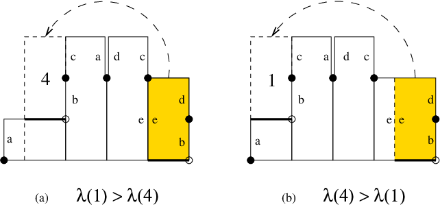
4 Interval exchanges with four intervals
For the rest of the paper we will consider interval exchanges on four intervals. Let where and . The extended Rauzy diagram is shown in Figure 3.

Now for each we form a pair of paths
and
that begin and end at . We form the corresponding product of elementary matrices and and set . One computes as follows. At each stage on the path, the marked permutation is determined from the previous marked permutation by (8) and (9). Each marked permutation determines an elementary matrix as in (9) and the discussion that follows. The matrix is the product of these elementary matrices. It is then easily verified that the entries of are polynomials in whose leading terms are
For each , set
For any , let be such that
Then successive applications of Rauzy induction on the interval exchange produces the interval exchange . Now let be the standard simplex in and regard each as a projective linear transformation from to itself.
Proposition 1.
The sets are a decreasing sequence with infinite intersection a single point denoted by . The interval exchange is uniquely ergodic.
In order to prove the proposition we use the Hilbert metric on . We will prove a general proposition stronger than what is needed. For any matrix with all positive entries set
Proposition 2.
Let be the open standard simplex in . Let be a sequence of projective linear transformation defined by positive matrices with
Then for any sequence of matrices with nonnegative entries,
is a single point.
Proof.
For define
and the Hilbert metric
Now for any matrix with nonnegative entries,
so it is enough to show that
Since the metric is a path metric, it is enough to show this inequality for arbitrarily small. By Lemma 15.2 of [F]
Writing , we see that the right hand side of the above expression is of the form
and so
which implies that
which gives the desired estimate. ∎
We now turn to the proof of Proposition 1. From the form of the leading terms of the matrix we compute that the entries of the matrix are all positive polynomials in whose leading terms are
We see immediately that there is an integer such that the entries of satisfy
for any , so that
Proposition 2 then implies that
as . Now it is a standard fact [K] that if is minimal, it is uniquely ergodic.
We now show that is minimal. Fix a unit area Abelian differential . (This means that the first return map of the vertical leaves to a horizontal segment defines the interval exchange and defines a zippered rectangle with height vector .)
If is not minimal then has a vertical saddle connection . Choose large enough so that does not intersect in its interior. This means that there is some rectangle in the ”zippered rectangles” determined by that has as part of its vertical side. In that case there would be a pair of zeros on a side which contradicts the zippered rectangle construction.
5 Proof of Theorem 1
We show that determines a divergent Teichmüller geodesic . To do that we need to show that for all sufficiently large times along the geodesic there is a simple closed curve which is short in the flat metric defined by .
The word that is used to form the matrix ends with . Recall that this means that the zippered rectangle for each interval exchange has a zero on the right side of the fourth rectangle. Thus there is a saddle connection such that the horizontal component of its holonomy is equal to , and such that the vertical component of its holonomy is at most . We will show that this saddle connection becomes short in some time interval and that these time intervals cover for large enough . Since has only one singularity, this saddle connection will always be a closed curve.
We first give a bound for . By (9) the length vectors satisfy the equation
and by (15) the height vector satisfies
| (18) |
The form of the leading terms of these matrices insures that for ,
| (19) |
and
| (20) |
Since
the above estimates show that
| (21) |
Moreover the form of the leading terms of the matrices also gives
which together with (19) and (21) gives
| (22) |
Now define by
| (23) |
and by
| (24) |
Now the flow contracts vertical holonomy by and expands horizontal holonomy by . By a slight abuse of notation we denote by , the saddle connection with respect to the Abelian differential .
These times are chosen so that for any
and
which implies that the length of is bounded by for any in this interval.
If we can show that the intervals and overlap, then we would be done, since this would imply that at all times there is a short saddle connection. By (22), (23),(24) and the fact that implies that
| (25) |
Now the form of the leading terms of the matrix implies that
(Here, means and .) Using (19) and the form of the leading terms of the matrix we have
so that
| (26) |
References
- [B] M. Boshernitzan, A condition for minimal interval exchange maps to be uniquely ergodic, Duke Math. J., v.52 (1985), no.3, 723–752.
- [F] H.Furstenberg, Stationary Processes and Prediction Theory Annals of Math Studies, 44 (1960).
- [K] M.Keane, Nonergodic interval exchange transformations Israel J.Math 141 (1977) 188-196.
- [Ke] S. Kerckhoff, Simplicial systems for interval exchange transformations and measured foliations, Ergodic Theory Dynamical Systems 5 (1985), 257-271.
- [KN] H. B. Keynes and D. Newton, A “minimal”, non-uniquely ergodic interval exchange transformation, Math. Z. 148 (1976), no. 2, 101-105.
- [M] H. Masur, Hausdorff dimension of the set of nonergodic foliations of a quadratic differential, Duke Math. J., 66 (1992), 387-442.
- [MMY] S. Marmi, P. Moussa, J.-C. Yoccoz, On the cohomological equation for interval exchange maps, arXiv:math.DS/0304469, 1 (2003), 1-11.
- [R] G. Rauzy, Echanges d’intervalles et transformations induites Acta Arith 34 (1979) 315-328.
- [S] E.Sataev, On the number of invariant measures of flows on orientable surfaces Izv. Acad. Sci. USSR 9 (1975) 860-878.
- [St] K. Strebel. Quadratic differentials. Springer-Verlag, (1984).
- [V1] W.Veech, Strict ergodicity in zero dimensional dynamical systems and the Kronecker-Weyl theorem mod 2, Trans. AMS, 140, (1969), 1-34.
- [V2] W.Veech Gauss measures for transformations on the space of interval exchange maps, Ann. Math. 115 (1982) 201-242.