Weight systems for Milnor invariants

A string link of $k$ components is a proper embedding of $k$ disjoint line segments into a solid cylinder so that each strand has one endpoint on the bottom and one on the top, and the order of the strands is the same at both ends. More formally, we have the following definition:

Note that any string link can be closed up to a link by joining the top and bottom of each component by an arc which lies outside of $D\times I$ (and which is unlinked with the other arcs). An isotopy invariant of string links is a map from the space of string links to some set which is invariant under ambient isotopies of the embedding of the line segments in the cylinder which leave the endpoints of the line segments fixed. A homotopy invariant is invariant under ambient isotopies, and also under crossing changes of a strand with itself (but not under crossing changes between two different strands).

We will also consider the more general notion of a $(l,2k-l)-tangle$, which has $k$ strands embedded in the cylinder $D\times I$ with $l$ endpoints arranged along the bottom of the cylinder and $2k-l$ along the top. So the order of the endpoints may be different on the top and bottom, or there may be strands which have both endpoints at the same end of the cylinder.

Roughly speaking, Milnor’s invariants detect how deeply the longitudes of the components of a string link lie in the lower central series of the link group.

Given a string link $L$, its link group $\pi_{1}((D^{2}\times I)-L)$ has a Wirtinger presentation, generated by the arcs of the string link diagram. We also have a presentation of the link group modulo the $q$th subgroup in its lower central series (see [5, 10]):

Note in particular that if component $j$ overcrosses all other components, then $\mu_{i_{1}...i_{n},j}$ is trivial, since the longitude $l_{j}$ will be the empty word. Also, if any component $i_{1},...,i_{n}$ undercrosses the other components, then its meridian will never appear in $l_{j}$, and $\mu_{i_{1}...i_{n},j}$ will likewise be trivial.

However, this definition can be rather unwieldy for computation. Polyak [11] has shown that the $\mu$-invariants without repeating indices (i.e. the homotopy invariants) satisfy a skein relation, similar to the skein relations for the Conway-Alexander and Jones polynomials, which provides another method of computation. Consider two string links (or oriented tangles) $L_{+}$ and $L_{-}$ which are identical except for one crossing of components $i_{k}$ and $j$, where $L_{+}$ has the positive crossing and $L_{-}$ has the negative crossing. We can ”split” this crossing in two ways to define two other oriented tangles. Let $L^{\prime}_{i_{k}}$ be a strand which follows $L_{j}$ (respecting orientation) until reaching the crossing, and then follows $L_{i_{k}}$ against the orientation. Let $L^{\prime}_{j}$ be a strand which follows $L_{i_{k}}$ and then switches to $L_{j}$, respecting the orientation on both components. Then we define $L_{0}=(L-L_{i_{k}}-L_{j})\cup L^{\prime}_{j}$ and $L_{\infty}=(L-L_{i_{k}}-L_{j})\cup L^{\prime}_{i_{k}}$ as shown in Figure 1.

Polyak showed that Milnor’s $\mu$-invariants satisfy the following skein relation:

In particular, in the cases when $k=1$ or $k=n$, we have:

So we can reduce any computation of $\mu$-invariants to a computation of linking numbers for tangles, which can be defined (using Gauss’s formula) as one-half the sum of the signs of the crossings (a positive crossing contributes +1, and a negative crossing -1). Since tangles may have an odd number of crossings, this will not always yield an integer, as it does for links and string links.

Notation: We will often consider the invariant $\mu_{1...n,n+1}$, or other invariants where the indices are a sequence of consecutive integers. For convenience, we will use $\mu_{i;j}$ to denote $\mu_{i,i+1,...,j-1,j}$.

Our treatment of finite type invariants will follow the combinatorial approach of Birman and Lin [4]. We will give a brief overview of this combinatorial theory; for more details, see [1, 4].

We first note that we can extend any tangle invariant to an invariant of singular tangles, where a singular $(l,2k-l)$-tangle is an immersion of a disjoint union of line segments in a solid cylinder (with $l$ endpoints on the bottom and $2k-l$ on the top) which is an embedding except for a finite number of isolated double points. We extend a tangle invariant $v$ to singular tangles via the relation in Figure 2

An invariant $v$ of singular tangles is then said to be of finite type, specifically of type n, if $v$ is zero on any tangle with more than $n$ double points (where $n$ is a finite nonnegative integer). We denote by $V_{n}$ the vector space over ${\mathbb{C}}$ generated by (framing-independent) finite type invariants of type $n$. We can completely understand the space of finite type invariants by understanding all of the vector spaces $V_{n}/V_{n-1}$. An element of this vector space is completely determined by its behavior on tangles with exactly $n$ singular points. In addition, since such an element is zero on tangles with more than $n$ singular points, any other (non-singular) crossing of the tangle can be changed without affecting the value of the invariant. This means that elements of $V_{n}/V_{n-1}$ can be viewed as functionals on the space of chord diagrams:

Functionals on the space of chord diagrams which are derived from finite type tangle invariants will satisfy certain relations. This leads us to the definition of a weight system:

The natural map from elements of $V_{n}/V_{n-1}$ to functionals on chord diagrams is a homomorphism into the space of weight systems [1, 4]. Kontsevich proved the much more difficult fact that these spaces are isomorphic [1, 7] (the inverse map is the famous Kontsevich integral). So we can take the dual approach, and simply study the space of chord diagrams of degree $n$ modulo the 1-term and 4-term relations.

When we are looking at homotopy invariants, such as the $\mu$-invariants, we can add another relation. Any homotopy invariant will vanish on a singular tangle with a double point where a component crosses itself, since the two resolutions differ only by a crossing change of the component with itself. This means that the associated weight system will vanish on any chord diagram that has a chord with both endpoints on the same component.

It is well-known that Milnor’s invariants are finite type invariants of string links [2, 8], but the proofs are rather complicated. We will use Polyak’s skein relation to give a simple combinatorial proof for the invariants without repeating indices.

Proof: The proof is by induction on $n$. It is well-known (and easy to prove) that the linking numbers $\mu_{i,j}$ are type 1. So we assume inductively that $\mu_{i_{1}...i_{k},j}$ is type $k$ for $k<n$, and consider a string link $L$ with $n+1$ double points. Without loss of generality, we can consider the invariant $\mu_{1...n,n+1}$, denoted $\mu_{1;n+1}$ (this is just a relabeling of the components). If none of the double points involves component $n+1$, we can look at the result of bringing component $n+1$ to the front (so it overcrosses all other components) by a series of crossing changes. The resulting string link $L^{\prime}$ has trivial $\mu_{1...n,n+1}$, and the difference between $L$ and $L^{\prime}$ is a linear combination of string links with $n+2$ double points, one of which involves component $n+1$. So it suffices to show that $\mu_{1...n,n+1}$ is trivial on any string link with at least $n+1$ double points, at least one of which involves component $n+1$. And any such link is a linear combination of string links with exactly $n+1$ double points (making sure to keep a double point involving component $n+1$).

So we may assume that $L$ has exactly $n+1$ singular crossings $c_{1},c_{2},...,c_{n+1}$, and that crossing $c_{n+1}$ involves components $n+1$ and $k$. Let $L_{e_{1},...,e_{n+1}}$, where $e_{i}=\pm 1$, be the string link resulting from resolving each singular crossing $c_{i}$ into a real crossing with sign $e_{i}$. Then:

Where the * indicates that the crossing has become a double point again. By continuing in this way, we will eventually obtain:

where $L_{S,\infty}$ has $c_{i}$ singular if $i\in S$ and negative otherwise, and $L_{S,0}$ has $c_{i}$ positive if $i\in S$ and singular otherwise.

By our inductive hypothesis, the terms of this sum will be trivial if $r>k-1$ or $n-r>n-k$. So the only non-trivial terms are when $r\leq k-1$ and $r\geq k$. But this is impossible, so all terms of the sum will be trivial, concluding the proof. $\Box$

We begin by making some useful observations about the connection graph of the chord diagram.

Proof: $C(D)$ is a graph with $n+1$ vertices and $n$ edges. If it is not a tree, then the graph must not be connected (since any connected graph with $n+1$ vertices and $n$ edges is a tree). So $D$ consists of two disjoint chord diagrams $D_{1}$ and $D_{2}$, where $D_{1}$ corresponds to the connected component of $C(D)$ containing vertex $n+1$, and $D_{2}$ is the remainder of the diagram. Recall that $M_{1;n+1}(D)=\mu_{1;n+1}(S(D))$, where $S(D)$ is any singular string link representing the chord diagram $D$ (this is well-defined since $\mu_{1;n+1}$ is type $n$). Choose $S(D)$ so that the components of $S(D_{1})$ are everywhere above the components of $S(D_{2})$; this is possible since there are no double points joining these sets of components. Then every term in the linear combination of string links represented by $S(D)$ has the components of $D_{1}$ lying above the components of $D_{2}$, so the longitude of component $n+1$ will not detect the components in $D_{2}$, and the word $l_{n+1}$ will not contain any of the meridians of the components in $D_{1}$. Therefore, $\mu_{1;n+1}$ is trivial on every one of these terms, and thus on $S(D)$. We conclude that $M_{1;n+1}(D)=0$, as desired. $\Box$

In particular, this means that (if $M_{1;n+1}(D)$ is non-trivial) $C(D)$ can have no multiple edges or loops, so $D$ cannot have multiple chords between two components, or chords with both endpoints on the same component. We should also observe that if $D$ has a chord with an endpoint on a component $r>n+1$, then $M_{1;n+1}(D)=0$, since $\mu_{1;n+1}$ cannot detect the difference in the two resolutions of the corresponding double point.

Recall from the proof of Theorem 1 that

On the level of weight systems, this means that

where $c$ is the chord between components $k$ and $n+1$, $J$ is a subset of the chords of $D-c$, $D_{J,\infty}$ is the chord diagram formed from $D$ by replacing components $k$ and $n+1$ by a new component $k$ as in Figure 4 and including the chords in $J$, and $D_{J,0}$ is the chord diagram formed from $D$ by replacing components $k$ and $n+1$ by a new component $n+1$ as in Figure 4 and including the chords in $(D-c)-J$.

The chords in $J$ must have both endpoints on components in $\{1,...,k,n+1\}$, and the chords in $(D-c)-J$ must have both endpoints on components in $\{k,k+1,...,n,n+1\}$. Since $c$ was the only chord between components $k$ and $n+1$ (by Lemma 1, there are no multiple chords between pairs of components), the chords in $J$ must have at least one endpoint on the chords $\{1,...,k-1\}$, and the chords in $(D-c)-J$ must have at least one endpoint on the chords $\{k+1,...,n\}$. So, in fact, the choice of $J$ is determined, and we have:

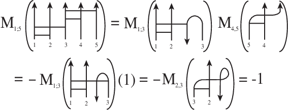
In particular, this product is trivial unless $|J|=k-1$, by Theorem 1. The product is also trivial if any chord in $D_{J,\infty}$ or $D_{J,0}$ has an endpoint on one of the ”erased” sections of components $k$ or $n+1$. Figure 5 shows how to use relation (1) to compute $M_{1;n+1}(D)$.

We will end this section with a useful lemma which uses Theorem 2 to give another sufficient condition for $M_{1;n+1}$ to be trivial.

Proof: Our proof will be by induction on $n$. Since $i,j,k,l$ are all distinct, $D$ must have at least 4 components, so our base case is $n=3$ ($n+1=4$). In this case $i=1$, $k=2$, $j=3$ and $l=n+1=4$. Applying relation (1) to $D$ using chord $b$, we get $M_{1;4}(D)=M_{1,2}(D_{J,\infty})\cdot M_{3,4}(D_{J,0})$, where $J$ is the set of chords with at least one endpoint on component 1. So chord $a$ is in $J$. But since the other endpoint of $a$ is on component 3, $M_{1,2}(D_{J,\infty})=0$, and so $M_{1;4}(D)=0$.

Inductively, we assume the lemma is true for $n<r$, and consider the case $n=r$. If $l=n+1=r+1$, we can apply relation (1) to chord $b$ and find that $M_{1;n+1}(D)=0$ as in the base case. If $l<n+1$, then there is a third chord $c$ with endpoints on components $m$ and $n+1$ (otherwise $C(D)$ is not connected, and $M_{1;n+1}(D)=0$ as in Lemma 1). We apply relation (1) to chord $c$. If $m>l$ then $D_{J,\infty}$ contains both chords $a$ and $b$, so $M_{1;m}(D_{J,\infty})=0$ by the inductive hypothesis. Similarly, if $m<i$ then $D_{J,0}$ contains both $a$ and $b$, so $M_{m+1;n+1}(D_{J,\infty})=0$. Otherwise we must have $i<m<j$ or $k<m<l$, in either case one of the chords $a$ or $b$ interlaces with chord $c$, so $M_{1;m}(D_{J,\infty})=0$ as in the base case. This completes the induction. $\Box$

We will show that the weight system $M_{1;n+1}$ depends only on the intersection graph of the chord diagram. The intersection graph for a tangle chord diagram is defined as follows:

Figure 6 shows an example of a chord diagram and its intersection graph.

Observe that the intersection graph $\Gamma(D)$ determines the connection graph $C(D)$, since $C(D)$ depends only on the labels of the vertices in $\Gamma(D)$. We will need the following lemma:

Proof: Since $C$ is a tree, every chord in $D_{1}$ and $D_{2}$ has its endpoints on different components, and two chords can share at most one component. This means that every edge in $\Gamma$ is directed. Hence, the relative positions of the endpoints along each component are determined by the directions of the edges in $\Gamma$, which completely determines the original chord diagram. $\Box$

By Lemma 1, if $\Gamma(D_{1})=\Gamma(D_{2})$ and $C(D_{1})=C(D_{2})$ is not a tree, then $M_{1;n+1}(D_{1})=M_{1;n+1}(D_{2})=0$. Together with Lemma 3, this gives us:

Using Theorem 2, we could also prove this by showing that we can obtain $\Gamma(D_{J,\infty})$ and $\Gamma(D_{J,0})$ from $\Gamma(D)$. This exercise is left to the reader. This approach also leads to the following useful corollary.

As a result of Corollary 1, we can ”redraw” chord diagrams as a different diagram with the same intersection graph, without changing the values of the Milnor weight system. In practice, we will often redraw tangle diagrams as string link diagrams (with disjoint parallel chords) in order to simplify our work.

We would like to have a better understanding of how the Milnor weight systems are related to intersection graphs. We will show that $M_{1;n+1}$ detects the presence of a certain kind of spanning tree - it is $\pm 1$ if this tree exists, and 0 otherwise. We will also see how the tree determines the sign.

We will begin by defining a special subgraph of the intersection graph of a chord diagram - the simplified intersection graph (or SIG). The idea of the SIG is to focus on the order of the chords along each component, and strip away any extraneous edges.

Proof: Let $D$ be a degree $n$ chord diagram on $n+1$ components, with $M_{1;n+1}(D)\neq 0$. Note that $SIG(D)$ must be connected - otherwise, either $C(D)$ is disconnected, or there are two chords with endpoints on the same components (so the edges between the vertices have cancelled ”mod 2”) and $C(D)$ has a loop. Either case contradicts Lemma 1.

We will first show that $SIG(D)$ is a tree. Assume $SIG(D)$ contains a loop $v_{1}v_{2}...v_{k}v_{1}$, where $v_{i}$ is labeled by $\{a_{i},b_{i}\}$; so $v_{i}$ corresponds to a chord $c_{v_{i}}$ with endpoints on components $a_{i}$ and $b_{i}$. We first consider the case when all the $a_{i}$’s are the same - i.e. all the chords have an endpoint on the same component. By Lemma 1, $C(D)$ is a tree, so no two chords can have the same labels; hence, all the $b_{i}$’s are distinct. Then the order of the chords along component $a=a_{i}$ is the same as the order of the vertices in the loop $v_{1}...v_{k}v_{1}$, which means that the chord $c_{v_{1}}$ is simultaneously above and below the chord $c_{v_{k}}$ along component $a$. This is impossible.

But if the $c_{v_{i}}$’s do not all have endpoints on the same component, then as we follow the loop we move from one component of $D$ to another, and ultimately return to the original component. This gives a loop in $C(D)$, which contradicts Lemma 1. So $SIG(D)$ must be a tree.

It remains to show that $SIG(D)$ is a rooted tree. We will show that every vertex has outdegree 1 except for one vertex (the root) which has outdegree 0, and that the root must have a label $\{i,n+1\}$. Then any directed path from any vertex must ultimately terminate at the root (since there are no loops). Assume there is a vertex $v$ (corresponding to chord $c_{v}$) with outdegree 0 and with label $\{i,j\}$, where $i<j<n+1$. If there is a vertex $w$ labeled $\{i,n+1\}$ or $\{j,n+1\}$ then we can apply relation 1 to the corresponding chord $c_{w}$. Since $v$ has outdegree 0, and $SIG(D)$ is connected, $c_{v}$ must be above $c_{w}$ along component $i$ (respectively, $j$). So after applying relation 1 to $c_{w}$, $c_{v}$ has an endpoint on an erased segment of $i$ (resp. $j$) in $D_{J,0}$ (resp. $D_{J,\infty}$). This means that $M_{1;n+1}(D)=0$, a contradiction.

If we do not have a vertex labeled $\{i,n+1\}$ or $\{j,n+1\}$, there will be some other vertex $u$ labeled $\{k,n+1\}$, $k\neq i,j$. The chord $c_{u}$ does not interlace $c_{v}$ by Lemma 2, so $c_{v}$ will be in either $D_{J,0}$ or $D_{J,\infty}$ when we apply relation (1) to $c_{u}$. By induction on the number of components, either $M_{1;k}D_{J,\infty}=0$ or $M_{k+1;n+1}D_{J,0}=0$; in either case $M_{1;n+1}(D)=0$, a contradiction. So any vertex with outdegree 0 must be labeled $\{i,n+1\}$ for some $i$. Since there is a directed path through the vertices with label $n+1$, there can be at most one such vertex; but since $SIG(D)$ is a tree, there must be at least one vertex with outdegree 0. We conclude that there is exactly one vertex with outdegree 0, and it has label $n+1$. This is the root $r$.

We still need to show that no vertex can have an outdegree greater than 1. Assume vertex $v$ has directed edges out to vertices $w$ and $u$. Then we can start at $v$ and follow a directed path through $w$ or through $u$. These paths must share some other vertex - if nothing else, they must both terminate at the unique root $r$. This would mean that $SIG(D)$ has a (undirected) loop, which is a contradiction. Therefore, except for $r$, every vertex has outdegree 1, and $SIG(D)$ is a rooted directed tree. $\Box$

While it is necessary that $SIG(D)$ be a rooted tree for $M_{1;n+1}(D)$ to be non-trivial, it is not sufficient. In the case when $SIG(D)$ is a rooted tree, we can define another spanning tree of $\Gamma(D)$ which we call the branched simplified intersection graph (BSIG). Unlike $SIG(D)$, the graph $BSIG(D)$ is dependent on the labels of the vertices (just as the Milnor invariants are dependent on the order of the indices). Before we define this new spanning tree, we will look at some implications of the simplified intersection graph being a tree.

For each component $i$ in $D$, let $r_{i}$ be the top chord on component $i$ in $D$ (and the corresponding vertex in $SIG(D)$). Note that only the root $r$ can be the top chord on two different components. Since every other chord has outdegree 1, every chord is a top chord on one component. Let $V_{i}$ be the set of vertices in $SIG(D)$ with label $\{i,j\}$ for some $j$. Then we can partition $V_{i}-\{r_{i}\}$ into two sets $L_{i}$ and $R_{i}$ (the left and right hand branches), where $L_{i}=\{\{i,j\}:j<i\}$ and $R_{i}=\{\{i,j\}:j>i\}$. If vertex $\{i,j\}$ is in $L_{i}$ or $R_{i}$, then it must be the top chord $r_{j}$ on component $j$, and vice versa; so the collection of the $L_{i}$’s and $R_{i}$’s is a partition of all the vertices of $SIG(D)$ except the root $r$. Obviously, $R_{n+1}$ is empty.

The branched simplified intersection graph takes each path in $SIG(D)$ through the vertices in $V_{i}$ and splits it into two paths - one through the vertices in $L_{i}$ and the other through the vertices in $R_{i}$ - joining the paths at $r_{i}$.

So $BSIG(D)$, when it exists, is also a rooted directed tree which is a spanning tree for $\Gamma(D)$. Figure 7 gives the branched simplified intersection graph for the chord diagram in Figure 6.

So the graph in Figure 7 is a good branched simplified intersection graph. We can now state the main result of this section.

For example, if $D$ is the chord diagram in Figure 6, with $BSIG(D)$ shown in Figure 7, then $L=|L_{2}|+|L_{4}|=2$, and $M_{1;8}(D)=(-1)^{2}=1$. We will prove this theorem in two parts. In Lemma 5 we show that if $D$ does not have a good $BSIG(D)$, then $M_{1;n+1}(D)=0$. In Lemma 6 we show that if $D$ does have a good $BSIG(D)$, then $M_{1;n+1}(D)=(-1)^{L}$.

Proof: If $BSIG(D)$ does not exist then $SIG(D)$ is not a rooted directed tree, so $M_{1;n+1}(D)=0$ by Lemma 4. So we can assume that $BSIG(D)$ exists, but that it fails one of the three conditions in Definition 8.

References

- [1] Bar-Natan, D.: On the Vassiliev Knot Invariants, Topology, Vol. 34, No. 2, 1995, pp. 423-472
- [2] Bar-Natan, D.: Vassiliev Homotopy String Link Invariants, J. of Knot Theory and its Ramifications, Vol. 4, No. 1, 1995, pp. 13-32
- [3] Bar-Natan, D. and Garoufalidis, S.: On the Melvin-Morton-Rozansky Conjecture, Invent. Math. 125, 1996, pp. 103-133
- [4] Birman, J. and Lin, X.S.: Knot polynomials and Vassiliev’s Invariants, Invent. Math. 111, 1993, pp. 225-270
- [5] Habegger, N. and Lin, X.S.: The Classification of Links up to Link-Homotopy, J. of the Amer. math. Soc., Vol. 3, No. 2, 1990, pp. 389-419
- [6] Habegger, N. and Masbaum, G: The Kontsevich Integral and Milnor’s Invariants, Topology, Vol. 39, No. 6, 2000, pp. 1253-1289
- [7] M. Kontsevich, Vassiliev’s knot invariants, Advances in Soviet Mathematics 16, Part 2, 1993, pp. 137-150
- [8] Lin, X.S.: Power Series Exapansions and Invariants of Links, Proceedings of the Georgia International Topology Conference, 1993
- [9] Mellor, B.: Intersection Graphs for String Links, preprint, 2003, arXiv:math.GT/0312347
- [10] Milnor, J.: Isotopy of Links, in Algebraic Geometry and Topology (edited by R. Fox), Princeton University Press, 1957, pp. 280-306
- [11] Polyak, M.: Skein Relations and Gauss Diagram Formulas for Milnor’s -invariants, preprint, 1999, http://www.math.tau.ac.il/ polyak/publ/skein.ps.gz