The space of doubly periodic minimal tori with parallel ends: Standard examples
Abstract. We describe a 3-parametric family of properly embedded minimal tori with four parallel ends in quotients of by two independent translations, which we will call the standard examples. These surfaces generalize the examples given by Karcher, Meeks and Rosenberg in [3, 4, 7]. can be endowed with a natural structure of a self-conjugated 3-dimensional real analytic manifold diffeomorphic to whose degenerate limits are the catenoid, the helicoid, the simply and doubly periodic Scherk minimal surfaces and the Riemann minimal examples. Pérez, Rodríguez and Traizet [9] characterize in the following sense: If is a properly embedded minimal torus in a quotient of by two independent translations with any number of parallel ends, then is a finite covering of a standard example.
1 Introduction
Scherk [10] presented in 1935 the first properly embedded minimal surface11 1 Unless explicitly mentioned, all surfaces in the paper are supposed to be connected and orientable. in , invariant by two linearly independent translations (we will shorten by saying a doubly periodic minimal surface). This surface is known as Scherk’s first surface, and fits naturally into a 1-parameter family of examples, called doubly periodic Scherk minimal surfaces. In the quotient by its more refined period lattice (i.e. the period lattice generated by its shortest period vectors), each has genus zero and four asymptotically flat annular ends: two top and two bottom ones, provided that the period lattice is horizontal. This kind of annular ends are called Scherk-type ends. The parameter in this family is the angle between top and bottom ends of . We can clearly consider the quotient of these by less refined period lattice to have two top and bottom ends for any natural , keeping genus zero in the quotient. Lazard-Holly and Meeks [5] proved that these are the only possible examples in this setting; i.e., if the quotient of a doubly periodic minimal surface has genus zero, then must be a doubly periodic Scherk minimal surface up to translations, rotations and homotheties. Moreover, the angle map is a diffeomorphism. Hence the moduli space of properly embedded minimal surfaces with genus zero in , a flat torus, is diffeomorphic to after identifying by rotations, translations and homotheties.
In 1988, Karcher [3] defined another -parameter family of doubly periodic minimal surfaces, called toroidal halfplane layers, with genus one and four Scherk-type parallel ends in its smallest fundamental domain (these examples will be denoted as in Section 2). Furthermore, he exposed two distinct -parameter deformations of each toroidal halfplane layer, obtaining other doubly periodic minimal tori with parallel ends (denoted as and , with , in Section 2). We generalize these Karcher’s examples in Section 2, by obtaining a -parameter family.
Theorem 1
There exists a -parameter family of properly embedded doubly periodic minimal surfaces with genus one and four parallel ends in the quotient by their more refined period lattices. This family can be endowed with a natural structure of a real analytic -dimensional manifold with the topology of the uniform convergence on compact sets. Furthermore:
- 1.
The isometry group of any surface is isomorphic to , or , depending on the values of , and it contains an orientation reversing involution without fixed points, producing a quotient Klein bottle with parallel ends.
- 2.
is self-conjugate, in the sense that the conjugate surface22 2 Two minimal surfaces are conjugate if the coordinate functions of are harmonic conjugate to the coordinate functions of . of any example in also belongs to .
- 3.
The possible limits of surfaces in are the catenoid, the helicoid, any singly or doubly periodic Scherk minimal surface, any Riemann minimal example or another surface in .
We refer to the examples in as standard examples. It is clear that we can consider quotients of the standard examples by less refined period lattices to have ends for any natural , keeping genus one. Pérez, Rodríguez and Traizet [9] have proved that these are the only possible examples in this setting.
Theorem 2
[9] If is a doubly periodic minimal surface with parallel ends and genus one in the quotient, then must be a standard example in up to translations, rotations and homotheties.
Meeks and Rosenberg [7] developed a general theory for doubly periodic minimal surfaces having finite topology in the quotient, and used an approach of minimax type to find theoretically some new examples with parallel ends and genus one in the quotient, besides those given by Karcher. After studying in detail the surfaces in , the uniqueness Theorem 2 assures that Meeks and Rosenberg’s examples are nothing but , for . Thus at least two of the most symmetric 1-parameter families in were known by Karcher [3, 4] and by Meeks and Rosenberg [7] (although our approach here is different from theirs). For this reason, the surfaces in also appear sometimes in the literature as KMR examples.
We will construct all standard examples as branched coverings of the sphere by their Gauss maps. The spherical configuration of a standard example, defined as the position in of the branch values of its Gauss map, allows us to read all the information concerning the minimal surface, see Section 2. Besides giving a unified method to produce all standard examples and studying their geometry, our motivation for writing this paper was to study the topology of .
Theorem 3
The space of properly embedded minimal surfaces with genus one and parallel ends in , a -dimensional flat torus, is diffeomorphic to .
The proof of Theorem 3 is inspired by the arguments of Pérez, Traizet and the author [9] to prove Theorem 2 (they follow the ideas of Meeks, Pérez and Ros [6]). We model the family of standard examples as an analytic subset in a complex manifold of finite dimension (roughly, consists of all admissible Weierstrass data for our problem). In the boundary of in , we can find the -parameter family of singly periodic Scherk minimal surfaces [3, 10]. We consider the classifying map , defined on , which associates to each surface in two geometric invariants: its period at the ends and its flux along a nontrivial homology class with vanishing period vector. Theorem 3 is a simple consequence of the following statements:
- 1.
is a proper map.
- 2.
is a local diffeomorphism.
- 3.
There exists such that consists of only one surface in .
- 4.
is a proper, divergent curve in .
The paper is organized as follows. In Section 2 we study the family of standard examples. Section 3 is devoted to introduce the space of admissible Weierstrass data and the classifying map that we use as a tool to demonstrate Theorem 3, and we prove that is a proper map. The goal of Section 4 is to prove the second statement above; i.e. is a local diffeomorphism. Finally, it can be found in Section 5 the proof of Theorem 3.
I sincerely want to thank Joaquín Pérez for his invaluable hepl along these years, and for leading me through this work.
2 Standard examples (proof of Theorem 1)
We dedicate this section to introduce the -parameter family of standard examples appearing in Theorem 1, to which the uniqueness Theorem 2 applies. First, let us point out some general facts. Let be a doubly periodic minimal surface with period lattice . Such induces a properly embedded minimal surface in the complete flat -manifold , where is a -dimensional flat torus. Reciprocally, if is a properly embedded nonflat minimal surface, then its lift is a connected doubly periodic minimal surface, by the Strong Halfspace Theorem of Hoffman and Meeks [2]. Assume that the topology of is a finitely punctured torus and that its ends are parallel. Then Meeks and Rosenberg [7] ensure that has finite total curvature and Scherk-type ends, for some natural . Therefore is conformally equivalent to a torus minus punctures. If we consider to be the more refined period lattice of , then Theorem 2 implies that .
Since has finite total curvature, its Gauss map extends meromorphically to . After a rotation so that the ends of are horizontal, takes values at the punctures, and the third coordinate function (which is not well-defined on ) defines an univalent holomorphic -form on , which we will call the height differential. Meeks and Rosenberg [7] proved that one of the meromorphic differentials has a simple pole at each puncture. As has no zeros on (it has no poles), we conclude that is unbranched at the ends, and has degree two. The Riemann-Hurwitz formula implies that the total branching number of is four.
Any standard example will be given in terms of the branch values of its Gauss map, which will consist of two pairs of antipodal points in the sphere . We label those points so that , . Since the Gauss map is unbranched at the ends (which are horizontal), we impose these branch values to be different from the North and South Poles. We denote by the equator that contains and by the point that bisects the angle between and , . We will call a spherical configuration to any set as above.
2.1 Toroidal halfplane layers
With the notation above, given we set the equator to be the inverse image of the imaginary axis through the stereographic projection from the North Pole, and , see Figure 1 left.

After stereographic projection we have , with , and the remaining branch values of the Gauss map of the example we are constructing are the four roots of the polynomial . Thus the underlying conformal compactification of the potential surface is the rectangular torus
The degree two extended Gauss map of is , the punctures correspond to , and the height differential must be for certain .
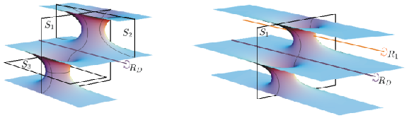
We consider . Then the set corresponds on to two closed horizontal geodesics which are the fixed point set of reflection symmetries in two horizontal planes (the reflection in both planes induce the same isometry of the quotient surface); the set corresponds on to four geodesics traveling from a zero to a pole of the Gauss map , which are the fixed point set of a reflection symmetry across two planes orthogonal to the -axis; and the set corresponds to two geodesics which are the fixed point set of a reflection symmetry in a vertical plane orthogonal to the -axis. The later geodesics cut orthogonally four straight lines parallel to the -axis and contained in , which correspond to the set . We will denote by the -rotation around any such straight line, see Figure 4 left.
We now construct a different model of , as a quotient of the -plane over a rectangular lattice. Let be one of the two components of . is topologically a disk and its boundary contains the branch point corresponding to the branch value of and one of the ends corresponding to a pole of . Let be an open rectangle in the -plane of consecutive vertices with the segment being horizontal, such that there exists a biholomorphism with boundary values , , and . Then the composition of with defines a biholomorphism between and . After symmetric extension of this biholomorphism across the boundary curves we will get a biholomorphism from to the quotient of the -plane modulo the translations given by four times the sides of the rectangle . We abuse the notation by labeling also the points of the -plane that correspond to the branch values of . The deck transformation of corresponds in the -plane to the -rotation about the branch points of . It will be also useful to see as a branched covering of through the map , i.e. two copies of glued along common cuts from to and from to , both contained in the imaginary axis.
In the -plane model of , corresponds to the reflection across the line passing through (or across its parallel line after translation by half a horizontal period, see Figure 1 right); is the reflection across the line passing through (or across its parallel line after translation by half a vertical period); is the reflection across the line passing through (or through ); and is the reflection across the line passing through (or through ). It is easy to see that Iso coincides with the group of conformal transformations of the underlying conformal torus , which is isomorphic to with generators .
Remark 1
All surfaces to be defined will have the same conformal compactification as . So from now on the sixteen elements in Iso generated by will be seen as conformal transformations of . Those that leave invariant the distribution of zeros and poles of the Gauss map of will be precisely the isometries of this last surface.
Concerning the period problem for , let be the simple closed curves in obtained as quotients of the horizontal and vertical lines in the -plane passing through and through respectively (see Figure 1 right). Clearly is a basis of . We normalize so that , which determines or, equivalently, the value of ,
| (1) |
where , , is the complete elliptic integral of the first kind. With this choice of , the period and flux vectors of along a small loop around the end of are respectively
| (2) |
The remaining ends of are
see Figure 1 right. From the behavior of the Weierstrass form under pullback by , one obtains that
| (3) |
where denotes the residue at the point . Note that (2) and (3) determine completely the periods and fluxes at :
| (4) |
Similar arguments imply that the periods and fluxes along the homology basis are
| (5) |
where
| (6) |
From equations (2), (4) and (5) we conclude that is a complete immersed minimal surface invariant by the rank two lattice generated by . Moreover, has genus one and four horizontal Scherk-type ends in the quotient, and can be decomposed in 16 congruent disjoint pieces. Karcher [3] proved that each of these pieces is the conjugate surface of certain Jenkins-Serrin graph defined on a convex domain. In particular, is embedded.
Next we study the limit surfaces of the examples in the family . When goes to zero, the function diverges to . After changing variables for with , it is easy to see that degenerates as into two spheres . The limiting Gauss map of as is and the height differential of converges smoothly to . Hence, when , the example converges smoothly to two vertical catenoids with flux , see Figure 2 left.
If , then and degenerates into two spheres . In this case, the limiting Gauss map is and the height differential collapses to zero because the limit of when vanishes. After scaling, it holds that as . Therefore, after blowing up, converges smoothly as to two doubly periodic Scherk minimal surfaces with two horizontal and two vertical ends, see Figure 2 right.

2.2 The examples
Given , and with , we consider the equator to be the rotated image of the imaginary axis in the sphere by angle around the -axis. If we denote by the rotated point by angle around the -axis of the North Pole, then our new point will be the rotation of by angle along , see Figure 3 left. Note that when , then coincides with the North Pole, which is not allowed in this setting. Also note that the spherical configuration associated to is nothing but the rotated image of that of by the Möbius transformation corresponding to the composition of the rotation of angle around the -axis with the rotation of angle around the -axis.

Consequently, we define the Gauss map of the standard example we want to construct as , i.e.
for , where and . Since depends analytically of , the same holds for its zeros and poles. We will denote by the ends of , understanding that each zero or pole of is defined by analytical continuation of the corresponding zero or pole of . Choosing the same homology class as in Subsection 2.1, we obtain that the height differential of is , with as in (1). Thus, the Weierstrass data of coincides with those of when .
The group Iso of isometries of the induced metric by always contains the deck transformation (we follow the notation in Subsection 2.1, see Remark 1). Furthermore, the antipodal map in leaves invariant the spherical configuration of , so Iso also contains two antiholomorphic involutions without fixed points, and . It is straightforward to check that we can label , and hence . This information is enough to solve the period problem for .
The period and flux vectors of at the end are given by
| (7) |
where we have used the identification of with by , and
The periods and fluxes at the remaining ends , and can be obtained from the equations in (4), which are still valid.
We choose the homology classes as in Subsection 2.1 (note that we can even take the same curve representatives as in the case except when or ). In particular, the third coordinate of the period of along equals , given by (6), so are linearly independent. It also holds
| (8) |
where denotes the Weierstrass form for . Equalities in (8) and (3) imply and , from which we deduce
| (9) |
All of these facts imply that is a complete immersed minimal torus invariant by the rank two lattice generated by , which has four horizontal Scherk-type ends in the quotient. Since is embedded and the heights of the ends of depend continuously on , which are in the connected set , we deduce that is embedded outside a fixed compact set. This fact together with a standard application of the Maximum Principle ensure that is embedded for all values of .
We next discuss what is the list of isometries of for different values of . As we mentioned above, Iso always contains the subgroup , which is isomorphic to with generators , . The deck transformation represents in a central symmetry about any of the four branch points of , and consists of a translation by . In particular, the ends of are equally spaced. If and , then the puncture lies on the open rectangle , see Figure 3 right. By Remark 1, Iso does not contain either for these values of , and so Iso. Thus it remains to study the special cases and .
- 1.
The case was studied in Subsection 2.1.
- 2.
Suppose that and , . In the -plane model of , the puncture moves vertically from its original position at the upper left corner of when downwards until collapsing for with the branch point ; next it goes on moving horizontally to the right until reaching the lower right corner of for , see Figure 3 right. The group of isometries Iso is isomorphic to with generators . Here represents in (as in Subsection 2.1) a reflection symmetry across a plane orthogonal to the -axis, and corresponds to a -rotation in around a line parallel to the -axis that cuts the surface orthogonally. When (resp. ), contains four (resp. two) straight lines parallel to the -axis, see Figure 4 right (resp. Figure 5 left). In both cases, is the -rotation around any of such line.
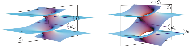
Figure 5: Left: for and . Right: for and . - 3.
In the case , , the puncture coincides with the lower right corner of , and Iso Iso. The isometry represents in a reflection symmetry across a plane orthogonal to the -axis. In this case, (resp. ) represents in a -rotation around one of the four (resp. two) straight lines parallel to the -axis (resp. -axis) contained on , see Figure 5 right.
- 4.
If and , then is an isometry of , since moves from the lower right corner of to its upper right corner, as varies from to . And Iso is isomorphic to with generators . Now represents in a -rotation around any of the four straight lines parallel to the -axis contained on , and is the composition of a reflexion symmetry across a plane orthogonal to the -axis with a translation by half a horizontal period, see Figure 6.

Figure 6: The standard example . - 5.
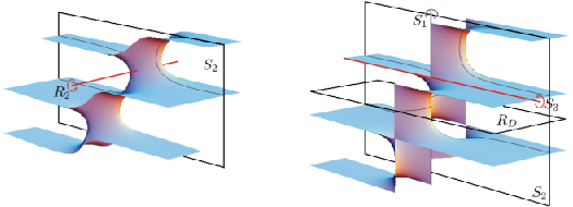
Suppose now that and . The puncture moves horizontally to the right running along the upper boundary side of . Thus Iso is isomorphic to , with generators , , . As in the case of , represents in space a reflection symmetry across two planes orthogonal to the -axis, and is a -rotation around a line parallel to the -axis that cuts orthogonally, see Figure 7 left.
- 6.
If , then is nothing but the rotated image of by angle around the -axis, hence we reduce the study to . Now lies on the upper right corner of , so all leave invariant the distribution of zeros and poles of the Gauss map of , and IsoIso. represents a reflection symmetry across two planes orthogonal to the -axis, (resp. ) represents in a -rotation around one of the four (resp. two) straight lines parallel to the -axis (resp. -axis) contained on , and corresponds to a reflection symmetry across two horizontal planes, see Figure 7 right.
Lemma 1
With the notation above, if and only if .
Proof.From (5) we know that when . Now suppose that and let us conclude that both and vanish.
If , is an isometry of , and we have and . Moreover, we obtain from (4) and (7) that and , with . Thus
and the second component of equals , which is not possible. Hence it must be . Since differs from in a rotation about the -axis, it also holds . This is, , and we can choose for every the same curve representative as in the case (i.e. ).
Since , then , and
| (10) |
Therefore, we deduce from that
The only possibility is then , and equation (10) reduces to
which is equivalent to
which only is satisfied for . Hence , as we wanted to prove.

We finalize this subsection by listing all the possible degenerate limits of the standard examples , all of which can be directly computed by using the Weierstrass data.
- •
When , for some , converges smoothly to a Riemann minimal example.
- •
When and , converges smoothly to two catenoids with flux , see Figure 2 left.
- •
When and , converges smoothly to two copies of the singly periodic Scherk minimal surfaces with four ends, two of them horizontal, and with angle33 3 We will call the angle of any singly or doubly periodic Scherk minimal surface to the angle between its nonparallel ends. , see Figure 8.
- •
When and , converges smoothly (after blowing up) to two vertical helicoids spinning oppositely, see Figure 9.

Figure 9: for and . - •
When and , converges smoothly (after blowing up) to two copies of the doubly periodic Scherk minimal surfaces with four ends, two of them horizontal, and with angle , see Figure 2 right.
Remark 2
We have defined the -parametric family of doubly periodic minimal surfaces, with , and in this range of parameters the end runs entirely along the closure of except its lower left corner . can be identified conformally through the -map with an octant of . We can easily extend the range of parameters so that runs entirely the sphere minus the branch values of the -map, which can be achieved by varying in . We can define for similarly as for , but it is straightforward to check that, up to translations, rotations and homotheties:
- •
coincides with , which does not depend on .
- •
is the reflected image of with respect to a plane orthogonal to the -axis.
- •
coincides with .
- •
is the reflected image of with respect to a plane orthogonal to the -axis.
Therefore, we define the family of standard examples as , where
| (11) |
We choose this space of parameters to avoid repeating surfaces twice, see Remark 2.
Remark 3
By construction, the branch values of the Gauss map of are contained in a spherical equator of , so a consequence of Theorem 14 in [8] assures that the space of bounded Jacobi functions on coincides with the space of linear functions of , (in particular, such space is -dimensional). This condition is usually referred in literature as the nondegeneracy of , which can be interpreted by means of an Implicit Function Theorem argument to obtain that is a -dimensional real analytic manifold (Hauswirth and Traizet [1]).
2.3 The space of standard examples is self-conjugate
In the previous subsection we have defined the family of standard examples. Given with Weierstrass data , we let denote the conjugate surface of , with Weierstrass data . Taking into account that the flux vector (resp. the period vector) of the conjugate surface along a given curve in the parameter domain equals the period vector (resp. the opposite of the flux vector) of the original surface along the same curve, we deduce from (4), (7) and (9) that is a complete immersed torus invariant by the rank two lattice generated by the horizontal vector and (whose third coordinate is ) and which has four horizontal Scherk-type ends in the quotient. Moreover, is embedded thanks to the Maximum Principle, since the heights of its ends depend continuously on , and is embedded (it is constructed from congruent blocks being Jenkins-Serrin graphs).
Note that, by (9), the period vector of along vanishes, and that the third component of the flux of along equals given by (6). The next lemma ensure that, after scaling and rotating the surfaces around the -axis, the families and coincide, which finishes the proof of Theorem 1.
Lemma 2
Given , the surface coincides with up to normalizations.
Proof.It is easy to see that . Since the Möbius transformation takes the set of branch points of the -projection of bijectively to the set of branch points of the -projection of , it follows that is a biholomorphism between and . On the other hand, it is straightforward to check that , where the subindex means the parameters of the standard example for which the corresponding is the Gauss map. Denoting by its height differential (recall that it only depends on ) a direct computation gives . Hence up to normalizations. Since by Remark 2, the lemma is proved.
3 The classifying map
The surfaces in can be naturally seen inside the 4-dimensional complex manifold consisting roughly of all admissible Weierstrass data in the setting of Theorem 2.
Definition 1
We denote by the space of tuples , where is a degree two meromorphic map defined on a torus which is unbranched at its zeros and at its poles , and is a homology class in , which is not trivial in .
See [9] for a detailed description of . We will shorten the elements in simply by , and call them marked meromorphic maps. Each determines a unique holomorphic differential on such that
| (12) |
since the complex space of holomorphic differentials on has dimension one. Thus each can be seen as the Weierstrass data , defined on , of a potential surface in the setting of Theorem 2. Equation (12) means that the period vector of along is horizontal and its flux along has third coordinate .
Definition 2
We will say that closes periods when the next equations hold
| (13) |
Note that the first equation in (13), together with (12), says that and . The next lemma justifies the above definition of closing periods.
Lemma 3 ([9])
If closes periods, then is the Weierstrass pair of a properly immersed minimal surface , for a certain flat torus , with total curvature and four horizontal Scherk-type ends. Furthermore, the fluxes at the ends are equal to for the positive real number appearing in (13), .
Next we describe how to see each standard example as an element of which closes periods. In a first step we rotate about the -axis so that the period at its end (we follow the notation in Section 2) is for certain . Now we associate to the marked meromorphic map
where everything has been already defined in Subsection 2.2 except the homology class . Recall that the ends depend continuously on and that we described explicitly the loop for . For the remaining values of , we take a embedded closed curve depending continuously on so that remains constant in .
3.1 The ligature map
We call ligature map to the holomorphic map defined as follows
which clearly distinguishes when a marked meromorphic map closes periods:
A marked meromorphic map closes periods if and only if there exist and such that .
Since the residues of a meromorphic differential on a compact Riemann surface add up to zero, if the second equation in (13) holds, then .
Let be the 1-dimensional moduli space of singly periodic Scherk minimal surfaces with two horizontal ends, vertical part of the flux at its two nonhorizontal ends equals to and period vector in the direction of the -axis. For each , let the singly periodic Scherk surface of angle . The limiting normal vectors of at its nonhorizontal ends project stereographically to . Recall we can obtain two copies of by taking limits from standard examples, see Subsection 2.2. We identify with the list , where:
- •
is a Riemann surface with nodes constructed by gluing two copies of with nodes .
- •
is the map which associates to each point in its complex value as a point in , (in particular, the degree of equals two).
- •
are respectively the zero and infinity in , .
- •
is an embedded closed curve in the homology class , where (resp. ) is a small loop in around (resp. ) with the positive orientation.

With the above identification, we can see in . From Lemma 6 and Theorem 2 of [9], one deduces that is a -dimensional complex manifold where extends holomorphically, and this extended ligature map is a biholomorphism in a small neighborhood of in . A straightforward computation gives us
| (14) |
3.2 The classifying map
In this subsection we will study the topology of the space , and the key ingredient for this study will be the classifying map that associates roughly to each marked standard surface its period at the ends and the horizontal component of its flux along a nontrivial homology class with zero period vector.
Definition 3
We denote and define the classifying map by so that and (hence ), provided that and is the height differential of .
Let be a marked surface in , and . Denote by a small loop around , oriented positively. If with , then , see Lemma 3. Since we want to avoid associating more than one different image to the same geometrical surface, it is necessary to restrict
Recall that is a 3-dimensional real analytic manifold, see Remark 3. It is clear from the definition above that is smooth. Also note that is essentially . Since extends as a biholomorphism in a small neighborhood of in , it follows that can be endowed with a structure of a 3-dimensional real analytic manifold and is also smooth. Remark that is not proper, since is contained in the boundary of in but . In detail, from (14) we have
| (15) |
Proposition 1
The classifying map is proper.
Proof.Take a sequence so that converges to some point , and let us prove that a subsequence of converges to a surface in .
First suppose that, after passing to a subsequence, for every , and let , see (11), be the angles which determine the spherical configuration of . Extracting a subsequence, we can assume that . By equation (7) we deduce that equals the modulus of , and so:
- •
If , then . These limits correspond, after blowing up, to two vertical helicoids when and , or to two copies of a doubly periodic Scherk minimal surface otherwise, see Subsection 2.2.
- •
If , but and , then . These limits correspond to the vertical catenoid when , or to a Riemann minimal example otherwise.
Therefore, the only possibilities are:
- •
and , and then converges to two copies of a singly periodic Scherk minimal surface.
- •
, so converges to the standard example .
- •
, hence (see Remark 2).
- •
, hence .
Hence admits a subsequence converging in (this can be also obtained by arguing as in the proof of Theorem 5 in [9]).
4 The classifying map is a local diffeomorphism
Proposition 2
The classifying map is a local diffeomorphism.
Proof.The relationship between and allows us to assure that is a diffeomorphism in a small neighborhood of in . Thus it only remains to demonstrate that is a local diffeomorphism. Consider a standard example and denote by its lifting to . It suffices to check that if is a Jacobi function that lies in the kernel of , then .
We can write for certain variation of . Let be the period lattice of , and . Since , then
| (16) |
By Lemma 2 and after normalizations, the conjugation map , which associates to each standard example its conjugate surface, is a well-defined map. Furthermore, is clearly differentiable since it is the restriction to of the map on the space of allowed Weierstrass data. Since clearly identity, then we deduce that is a diffeomorphism. Hence it suffices to prove that the tangent vector defined as the image of by the differential of , vanishes identically. Notice that , being the conjugate surface of . In particular, is a Jacobi function on , which is moreover bounded since all the have horizontal ends.
First suppose that is a bounded Jacobi function on the quotient of by its period lattice. By Remark 3 we know that is of the kind , for some . Theorem 3 in [8] assures that there exists a unique element of the space of complete branched minimal immersions into (including the constant maps) with finite total curvature and planar ends whose extended Gauss map is , such that . Thus is constantly , and corresponds to a translation of in . As we are considering the surfaces in up to translations, it holds . Therefore it only remains to prove that descends to the quotient .
Recall that the flux of at its ends is (up to sign) and its flux along the homology class in the last component (viewed as a marked standard example) is . Therefore the period lattice of (before normalization) is generated by and . We parameterize by , and denote by the diffeomorphisms induced by , i.e. those satisfying
| (17) |
By (16), . Therefore,
Analogously . Thus descends to the quotient and Proposition 2 is proved.
5 The topology of (proof of Theorem 3)
By Propositions 1 and 2, is a proper local diffeomorphism, and so a finite sheeted covering map. We deduce from Lemma 1, Remark 2 and equation (15) that the only surfaces with , for some , are the standard examples . Since is a strictly decreasing function in , the number of sheets of the covering map is one, and so it is a diffeomorphism. Moreover, the set consists of the proper arc , from where it follows that is diffeomorphic to the complement in of such arc, which in turn is diffeomorphic to . This proves Theorem 3.
Remark 4
Since is a diffeomorphism, any standard example is completely determined by its image through . This justifies the words classifying map for .
Recall that we can identify some standard examples in by symmetries (see Remark 2). Since there are standard examples invariant by such symmetries, we deduce that the quotient of by these symmetries has structure of -dimensional orbifold. Notice that this quotient space is the moduli space of doubly periodic minimal surfaces with parallel ends and genus one in the quotient.
M. Magdalena Rodríguez at magdarp@ugr.es
References
- [1] L. Hauswirth and M. Traizet. The space of embedded doubly-periodic minimal surfaces. Indiana Univ. Math. J., 51(5):1041–1079, 2002. MR1947868.
- [2] D. Hoffman and W. H. Meeks III. The strong halfspace theorem for minimal surfaces. Invent. Math., 101:373–377, 1990. MR1062966, Zbl 722.53054.
- [3] H. Karcher. Embedded minimal surfaces derived from Scherk’s examples. Manuscripta Math., 62:83–114, 1988. MR0958255, Zbl 658.53006.
- [4] H. Karcher. Construction of minimal surfaces. Surveys in Geometry, pages 1–96, 1989. University of Tokyo, 1989, and Lecture Notes No. 12, SFB256, Bonn, 1989.
- [5] H. Lazard-Holly and W. H. Meeks III. Classification des surfaces minimales de genre zéro proprement plongées dans . Comptes–Rendus de l’Académie des Sciences de Paris, pages 753–754, 1997.
- [6] W. H. Meeks III, J. Pérez, and A. Ros. Uniqueness of the Riemann minimal examples. Invent. Math., 131:107–132, 1998. MR1626477, Zbl 916.53004.
- [7] W. H. Meeks III and H. Rosenberg. The global theory of doubly periodic minimal surfaces. Invent. Math., 97:351–379, 1989. MR1001845, Zbl 676.53068.
- [8] S. Montiel and A. Ros. Schrödinger operators associated to a holomorphic map. In Global Differential Geometry and Global Analysis (Berlin, 1990), volume 1481 of Lecture Notes in Mathematics, pages 147–174. Springer-Verlag, 1991. MR1178529, Zbl 744.58007.
- [9] J. Pérez, M. M. Rodríguez, and M. Traizet. The classification of doubly periodic minimal tori with parallel ends. J. of Differential Geometry, 69(3):523–577, 2005. MR2170278, Zbl pre05004289.
- [10] H. F. Scherk. Bemerkungen über die kleinste Fläche innerhalb gegebener Grenzen. J. R. Angew. Math., 13:185–208, 1835.