We consider hashing with linear probing for a hashing table with a set of $m$ places, $\{1,2,...,m\}$, $n$ items $\{c_{1},c_{2},...,c_{n}\}$, and $\ell=m-n$ empty places ($\ell>0$). Hashing with linear probing is a fundamental object in analysis of algorithms: its study goes back to the 1960’s [29, 31] and is still active [2, 23, 30, 42]. For a non computer science-minded reader, we shall use, all along the paper, the metaphore of $n$ cars parking on $m$ places, leaving $\ell$ places empty: each car $c_{i}$ chooses a place $p_{i}$ at random, and if $p_{i}$ is occupied, $c_{i}$ tries successively $p_{i}+1$, $p_{i}+2$, until it finds an empty place. We use the convention that place $m+1$ is also place $1$.

Under the name of parking function, hashing with linear probing has been and is still studied by combinatorists [25, 26, 45, 49, 50, 51]. Section 4 of [23] contains nice developments on the connections between parking functions and many other combinatorial objects. In this paper, we use mainly a - maybe less exploited - connection between parking functions and empirical processes of mathematical statistics (see also [15, 39]) .

Let $B_{k}^{m,\ell}$ denote the size of the $k^{th}$ largest block of consecutive cars, and let $B^{m,\ell}=(B_{k}^{m,\ell})_{k\geq 1}$ be the decreasing sequence of sizes of blocks, ended by an infinite sequence of $0$’s. Pittel [42] proves that when $\ell/m$ goes to some positive limit $\beta$, $B_{1}^{m,\ell}$ satisfies

where $\Xi_{m}$ converges weakly to an extreme-value distribution. This paper is concerned with what we would call the ”emergence of a giant block”, by reference to the emergence of a giant component [4, 9, 14, 22, 28]. We have:

Thus a phase transition occurs for $\ell=\Theta(\sqrt{m})$. The main result of this paper is the description of this phase transition with the help of Brownian motion theory, following [4]. More precisely, as in [4], the asymptotic behaviour of blocks’ sizes is described by widths of excursions of stochastic processes related to the Brownian motion. It turns out, by nature of the problem, and also owing to previous works of Aldous & Pitman [8], that the description given here (specially by Theorem 1.3) is more precise than in [4].

Recall some notations and definitions from Brownian motion theory. An excursion (from $0$) of the function $f$ is the restriction of $f$ to an interval $[a,b]$ such that

$b-a$ is the width or length of the excursion, $a$ is the starting point (or the beginning) of the excursion, $b$ the end of the excursion. Let us adopt the notation of [54, Lecture 4] for the Brownian scaling of a function $f$ over some interval $[a,b]$:

If $f$ is the standard linear Brownian motion, and $g$ (resp. $d$) is the last zero of $f$ before $1$ (resp. the first zero of $f$ after $1$), then $e=\left|f^{[g,d]}\right|$ is called the normalized Brownian excursion. When it is convenient, we regard the normalized Brownian excursion $e(t)$ as defined on the whole real line, being periodic with period $1$. We define, for $\lambda\geq 0$, the operator $\Psi_{\lambda}$ on the set of bounded functions on the line by

If $f$ has period 1, then so has $\Psi_{\lambda}f$. Evidently, $\Psi_{\lambda}f$ is nonnegative, and we have

Let $B(\lambda)=(B_{k}(\lambda))_{k\geq 1}$ be the sequence of widths of excursions of $\Psi_{\lambda}e$, sorted in decreasing order. The sequence $B(\lambda)$ is a random element of the simplex

We have:

For instance, to complete Theorem 1.1, note that

Before we discuss the law of $B(\lambda)$, in the next Subsection, let us pursue the description of the asymptotics of the phase transition for parking blocks: up to now, we only considered the parking process frozen at a given time $n=m-\ell$, that is, just after the arrival of car $c_{n}$. The next Theorem describes the evolution of blocks’ sizes, as cars arrive, during the phase transition: asymptotically, the joint law of sequences of blocks’ sizes $B^{m,\lceil\lambda_{i}\sqrt{m}\rceil}$ after successive arrivals of cars $c_{n(i)}$, $n(i)=m-\lceil\lambda_{i}\sqrt{m}\rceil$, $\lambda_{1}>\lambda_{2}>\cdots>\lambda_{k}$, once these sequences are normalized, converges to the joint law of $\left(B(\lambda_{i})\right)_{i=1,2,...,k}$. More formally, set

We have:

Though, in the random graph model, the asymptotic distribution of sizes of clusters (connected components) has a description similar to that given at Theorem 1.2, the analog of Theorem 1.3 is false, as observed by Aldous [4]: in coalescence models based on excursions of stochastic processes, clusters (excursions) can only merge with their neighbors, while this is not true for connected components of the random graph. In Section 4, at the price of heavier notations, we give the analog of Theorem 1.3 for the asymptotic behaviour of sizes and positions of blocks.

As a consequence of [34, Theorem 4], we have

Theorem 4 of [34] gives the limit law of the largest tree in a random forest: it turns out that forests and parking schemes are in one-to-one correspondence (see Subsection 5.1). Flajolet & Salvy [24] have a direct approach, to the computation of the density of $B_{1}(\lambda)$, by methods based on Cauchy coefficient integrals to which the saddle point method is applied: the density they obtain is a variant of the Dickman function [52, Ch. III, Sec. 5.3].

In view of Theorem 1.4, the joint law of $(B_{1}(\lambda),B_{2}(\lambda),\,\dots\,,B_{k}(\lambda))$ seems out of reach, but we are more lucky with the joint law of the first terms of a sequence $R(\lambda)$ obtained by permutation of the terms of $B(\lambda)$. Roughly speaking, in the size-biased permutation $R(\lambda)$ of a random probability distribution such as $B(\lambda)$, the largest terms of the sequence $B(\lambda)$ appear with a high probability at the beginning of the sequence $R(\lambda)$: we have

the $k^{th}$ term of $R(\lambda)$ being also drawn randomly with a probability proportional to its size, but among the terms that did not appear before. A more formal definition of size-biased permutations, by construction through a rejection method, is given in [38]: consider a sequence of independent, positive, integer-valued random variables $(I_{k})_{k\geq 1}$, distributed according to $B(\lambda)$:

With probability $1$ the terms of $B(\lambda)$ are positive, as $\Psi_{\lambda}e$ has infinitely many excursions, so each positive integer appears at least once in the sequence $(I_{k})_{k\geq 1}$. Erase each repetition after the first occurence of a given integer in the sequence: there remains a random permutation $(\sigma(k))_{k\geq 1}$ of the positive integers. Set:

We have:

Actually, Theorem 1.5 gives an implicit description of the law of $B(\lambda)$, for instance it proves that almost surely each $R_{k}(\lambda)$ is positive, and thus a.s. $0<B_{k}(\lambda)<1$. Size-biased permutations of random discrete probabilities have been studied, among others, by Aldous [1] and Pitman [37, 38]. The most celebrated example is the size-biased permutation of the sequence of limit sizes of cycles of a random permutation. While the limit distribution of the sizes of the largest, second largest … cycle have a complicated expression [19, 47], the successive terms $R_{1},R_{2},~~...~~$ of their size-biased permutation satisfies

in which the $U_{k}$ are uniform on $[0,1]$ and independent. Actually, it is common that the distribution of the size-biased permutation of a sequence has a simpler distribution than the original sequence, when the sequence is related to a Poisson point process, a famous example being the Poisson-Dirichlet distribution [10, 11, 35, 36, 41]. The distribution of $R(\lambda)$, as described in Theorem 1.5, already appeared as the law of the $\Delta$-valued fragmentation process derived from the continuum random tree, introduced by Aldous & Pitman in their study of the standard additive coalescent [8, Corollary 5]: this is commented in the next Subsection.

As in the case of sizes of cycles, the unnatural size-biased permutation of $B(\lambda)$ is the limit of a natural permutation of $B^{(m)}(\lambda)$: define $R^{m,\ell}=\left(R_{k}^{m,\ell}\right)_{k\geq 1}$ as the sequence of sizes of blocks when the blocks are sorted by increasing date of birth (in increasing order of first arrival of a car). If $\ell\geq m$, or if there are less than $k$ blocks, set $R_{k}^{m,\ell}=0$. For instance, on Figure 1, $B^{m,\ell}=(3,3,1,0,\ \dots\ )$ and $R^{m,\ell}=(3,1,3,0,\ \dots\ )$. Concerning $R^{m,\ell}$, we have an analog of Theorem 1.2 :

Set

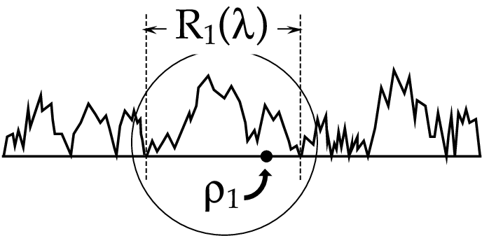
For an analog of Theorem 1.3 to hold true, giving the convergence of finite dimensional distributions of $R^{(m)}$, we should define $\left(R(\lambda)\right)_{\lambda\geq 0}$ as a process. This is not straightforward, as there are many possible definitions of the size-biased permutation $\sigma_{\lambda}$ that throws $B(\lambda)$ on $R(\lambda)$ : $\sigma_{\lambda}$ has to be defined as a process too. For sake of brevity, we shall only state a result for the first component of $R(\lambda)$. Consider a random number $\rho_{1}$, uniform on $[0,1]$ and independent of $e$, and define $R_{1}(\lambda)$ as the width of the excursion of $\Psi_{\lambda}e$ that contains $\rho_{1}$ (see Figure 3). Then $R_{1}(\lambda)$ is defined, and satisfies (1.2),

simultaneously for each value of $\lambda$. We have:

It turns out that the limit process has a rather simple description: set

We have

It is well known that the family of first hitting times of levels $\lambda$ by the Brownian motion is also the stable subordinator with exponent $1/2$. The following description of the stable subordinator with exponent $1/2$, by its finite dimensional distributions, will be useful for the proof: for any $k$ and any k-tuple of positive numbers $(\lambda_{i})_{1\leq i\leq k}$,

in which the $N_{k}$ are standard Gaussian and independent.

The well known fact that $\Sigma(\lambda)$ is a pure jump process makes sense in the parking scheme context, since the block of car $c_{1}$ is known to increase by $O(m)$ while only $O(\sqrt{m})$ cars arrived: it can only be explained by coalescence with other blocks of size $O(m)$, that is, by instantaneous jumps. Incidentally, let $L(\lambda)$ denote the length of the excursion of $\Psi_{\lambda}e$ beginning at $0$, and set

Bertoin [12] nicely proves that $(\Sigma,R_{1})$ and $(\tilde{\Sigma},L)$ have the same law. For the moment, we do not see any combinatorial explanation of this identity between $R_{1}$ and $L$.

We give here a brief account of coalescence, which is masterfully surveyed in [5, 6]. We essentially quote the two previously cited references. Models of coalescence (aggregation, coagulation, gelation …) have been studied in many scientific disciplines, essentially physical chemistry, but also astronomy, bubble swarms, mathematical genetics, and recently random graph theory [6, Section 1.4]. In a basic model, clusters with different masses move through space, and when two clusters (say, with masses $x$ and $y$) are sufficiently close, there is some chance that they merge into a single cluster of mass $x+y$ [6, Section 1.1]. The probability that they merge is quantified, in some sense, by a rate kernel $K(x,y)$. As far as parking is concerned, the growth of clusters (parking blocks) is due partly to cars’ arrivals, partly to aggregation with other blocks, but we saw that during the phase transition the coalescence factor is preponderant.

A complete model for coalescence, detailing mass, position, and velocity of each cluster, is too complicated for analysis, so recent works focused on the evolution of masses of clusters through time: the general stochastic coalescent [21] is the continuous-time Markov process whose state space is the infinite-dimensional simplex

(the $x_{i}$’s are the sizes of clusters) and that evolves according to the rule

It means that, if at time $t$ the state of the system is $(x_{i})_{i\geq 1}$, the next pair $(I,J)$ of clusters that will merge and the time $t+T$ when they merge are jointly distributed as follows: assume we are given a set of independent random variables $(T_{i,j})_{1\leq i<j}$ with distribution described by

and set

It turns out that the way connected components merge in the random graph process is somehow related to the multiplicative coalescent ($K(x,y)=xy$) [4]. One rather expects the parking to be related to the additive coalescent ($K(x,y)=x+y$): given that a parking scheme with $m$ places, $n$ cars and $\ell=m-n$ empty places has two blocks with size $x$ and $y$, the probability that these two blocks merge at the next arrival is

as the number of empty places after block $x$ but before block $y$ is random uniform on $1,2,\dots,\ell-1$, and, given that this number is $1$ (resp. $\ell-1$, $\notin\{1,\ell-1\}$) the conditional probability that the two blocks merge at the next arrival is $\frac{x+1}{m}$ (resp. $\frac{y+1}{m}$, $0$). Aldous & Pitman [8] give a construction of the additive coalescent through a fragmentation process $Y=\left(Y(\lambda)\right)_{\lambda\geq 0}$: the $\Delta$-valued random variable $Y(\lambda)$ is the ranked sequence of masses of tree components of continuum forests obtained by cutting the ”edges” of the Brownian continuum random tree by a Poisson process of cuts with rate $\lambda$ by unit length. As more or less expected, according to Theorem 1.5 and to [8, Corollary 5], the distributions of $Y(\lambda)$ and $B(\lambda)$ are the same.

Furthermore, let $\rho_{1}^{\star}$ be a leaf, of the Brownian continuum random tree, picked uniformly at random according to the mass measure, and let $Y_{1}^{\star}(\lambda)$ denote the mass of the tree component of the random forest that contains $\rho_{1}^{\star}$ when the cutting intensity is $\lambda$. Then, according to Theorem 1.8 and to [8, Theorem 6], the distributions of the stochastic processes $Y_{1}^{\star}$ and $R_{1}$ are the same. These facts suggest that

Theorem 1.9 is actually the main result of a recent paper by Bertoin [12]. In Section 7, we give an alternative proof of Theorem 1.9, that relies on Theorem 1.10, a path decomposition result for $\Psi_{\lambda}e$.

Note that Theorem 1.8 is not a mere consequence of Theorem 1.9 and [8, Theorem 6], as the very similar selection mechanisms leading to $Y_{1}^{\star}$ (resp. $R_{1}$) depend not only on the stochastic processes $Y$ (resp. $B$), but on underlying richer structures, a family of Poisson point processes of cuts of a Brownian continuum random tree on one hand, and the family of stochastic processes $\Psi_{\lambda}e$ on the other hand. Even if one of the constructions of the Brownian continuum random tree uses the normalized Brownian excursion [3, Corollary 22], we do not know for the moment any extension of Theorem 1.9 to these richer structures, that would yield a direct proof of the identity between the distributions of the stochastic processes $Y_{1}^{\star}$ and $R_{1}$. However, in the concluding remarks, we give a rather convincing combinatorial explanation of the connection between the two richer structures.

In previous subsections, objects from Brownian motion theory allowed to describe phase transition for parking schemes. In this subsection, we translate the parking schemes combinatorial identity:

to obtain Theorem 1.10, a property of decomposition of sample paths of $\Psi_{\lambda}e$ used in Section 7 to give simple proofs of Theorems 1.5, 1.8 and 1.9.

Let $\rho_{1}$ be a random variable uniformly distributed on $[0,1]$ and independent of $e$. Almost surely, $\Psi_{\lambda}e(\rho_{1})$ is positive. Let $g(\lambda)$ (resp. $d(\lambda)$) denote the last zero of $\Psi_{\lambda}e$ in the interval $[0,\rho_{1})$ (resp. the first zero in the interval $(\rho_{1},1]$), so that $R_{1}(\lambda)=d(\lambda)-g(\lambda)$. To avoid the extensive use of notation $\{x\}$ for the fractional part of the real number $x$, we shall extend $\Psi_{\lambda}e$, as well as other functions defined on $[0,1]$, such as $q$ or $r$ defined below, to periodic functions on the line. We set

Let $\tau_{x}$ denote the shift operator for functions on the line, defined by

Actually, not only the conditional distribution of $\tau_{w}r$, but also the conditional distribution of $r$ has a simple description in terms of the Brownian motion, and also as a nonuniform random shift of $\Psi_{\frac{\lambda}{\sqrt{1-x}}}e$ [16]. However, the weaker form $(iii)$ fills our needs for the proofs of Theorems 1.5, 1.8 and 1.9.

The paper is organized as follows. Section 2 analyses the block containing a given car or a given site, leading to the proof of Theorem 1.1. At Section 3, we give the proof of the main result, Theorem 1.2, with the help of a close coupling between empirical processes of mathematical statistics and the profile obtained by assuming that each car lays a $1/\sqrt{m}$-thick layer of sediment on the way between its first try and its final place (see Figure 5). We extend these arguments at Section 4 to obtain the asymptotic of the joint law, at different times, of widths and positions of blocks. Distributional results, Theorems 1.4 and 1.6, are proven at Section 5 by combinatorial arguments. We prove Theorems 1.7 and 1.10 at Section 6, with the help of Theorem 3.1, about weak convergence of profiles. Finally, in Section 7, Theorems 1.5, 1.8 and 1.9 are shown to be consequences of Theorem 1.10. Section 8 concludes the paper with an attempt of combinatorial explanation for the connections between our paper and [8].

Propositions 3.3 and 3.4, at the end of this subsection, are the key points for the convergence of blocks’ sizes. Given a sequence $(U_{k})_{k\geq 1}$ of independent uniform random variables, we assume that first try of car $c_{k}$ is place $\lceil mU_{k}\rceil$, all parking schemes being thus equiprobable. If $Y_{k}$ denotes the number of cars whose first try was place $k$, then we have:

since either place $k$ is occupied by car $c_{i}$ and, among the $H_{k}$ cars that tried place $k$, only car $c_{i}$ won’t visit place $k+1$, so that $H_{k+1}=Y_{k+1}+(H_{k}-1)$, or place $k$ is empty and $H_{k+1}=Y_{k+1}$. We understand this equation, when $k=m$, as $H_{1}=Y_{1}+(H_{m}-1)_{+}$. This induction alone does not give the $H_{k}$’s, since we do not have any starting value. The gap is filled by Proposition 3.2, that gives the connection between hashing (or parking) and empirical processes.

Given a sample $(U_{1},U_{2},...,U_{n})$ of uniform random variables, the empirical distribution $F_{n}$ and the empirical process $\alpha_{n}$ (see [18, 43, 48] for background) are respectively defined by

References

- [1] D. J. Aldous, Exchangeability and related topics. Ecole d’ete de probabilites de Saint-Flour XIII - 1983, Lect. Notes Math. 1117, 1-198 (1985).
- [2] D. Aldous, Hashing with linear probing, under non-uniform probabilities. Probab. Eng. Inform. Sci., 2, 1-14 (1988).
- [3] D. Aldous, The continuum random tree III. Ann. Probab. 21, 248-289 (1993).
- [4] D. J. Aldous, Brownian excursions, critical random graphs and the multiplicative coalescent. Ann. Probab. 25, No.2, 812-854 (1997).
- [5] D. Aldous, Stochastic coalescence. Documenta Mathematica, Extra Volume I.C.M. 1998, III, 205-211 (1998).
- [6] D. Aldous, Deterministic and stochastic models for coalescence (aggregation and coagulation): a review of the mean-field theory for probabilists. Bernoulli 5, No. 1, 3-48 (1999).
- [7] D. J. Aldous & Jim Pitman, Brownian bridge asymptotics for random mappings. Random Structures Algorithms 5, No. 4, 487-512 (1994).
- [8]
D. J. Aldous
&Jim Pitman, The standard additive coalescent. Ann. of Proba. 26, 1703-1726 (1998). - [9] N. Alon & J.H. Spencer, The probabilistic method. With an appendix by Paul Erdos. John Wiley & Sons, Inc., New York-London-Sydney (1992).
- [10] R. Arratia, A. D. Barbour & S. Tavaré, Poisson process approximations for the Ewens sampling formula. Ann. Appl. Probab. 2, No. 3, 519-535 (1992).
- [11] R. Arratia, A. D. Barbour & S. Tavaré, On Poisson-Dirichlet limits for random decomposable combinatorial structures. Combin. Probab. Comput. 8, No. 3, 193-208 (1999).
- [12] J. Bertoin, A fragmentation process connected to Brownian motion. Probab. Theory Relat. Fields 117, 289-301 (2000).
- [13] P. Billingsley, Convergence of Probability Measures. John Wiley & Sons, Inc., New York-London-Sydney (1968).
- [14] B. Bollobás, Random graphs. Academic Press, London-New York (1985).
- [15] P. Chassaing & J.F. Marckert, Parking functions, empirical processes and the width of rooted labeled trees. Electronic J. Combinatorics 8(1), R14 (2001).
- [16] P. Chassaing & S. Janson, A Vervaat-like path transformation for the reflected Brownian bridge conditioned on its local time at , Ann. Probab., October 2001.
- [17] P. Chassaing & G. Louchard, Phase transition for parking blocks, Brownian excursion and coalescence. Prépublication 99/34 de l’Institut Elie Cartan, Sep. 1999, available at: http://www.iecn.u-nancy.fr/chassain
- [18] M. Csörgö, P. Révész, Strong approximations in probability and statistics. Probability and Mathematical Statistics. Academic Press, Inc., New York-London (1981).
- [19] K. Dickman, On the frequency of numbers containing prime factors of a certain relative magnitude. Ark. Mat. Astronomi och Fysik 22, 1-14 (1930).
- [20] M. D. Donsker, Justification and extension of Doob’s heuristic approach to the Kolmogorov-Smirnov theorems. Ann. Math. Statistics 23, 277-281 (1952).
- [21] S. N. Evans & J. Pitman, Construction of Markovian coalescents. Ann. Inst. Henri Poincaré 34, No. 3, 339-383 (1998).
- [22] P. Flajolet, D.E. Knuth & B. Pittel, The first cycles in an evolving graph., Graph theory and combinatorics (Cambridge, 1988). Discrete Math. 75, No. 1-3, 167-215 (1989).
- [23] P. Flajolet, P. Poblete, A. Viola, On the Analysis of Linear Probing Hashing, Algoritmica Vol. 22, No. 4, 490-515 (1998).
- [24] Ph. Flajolet & B. Salvy, private communication.
- [25]
D. Foata,
&J. Riordan, Mappings of acyclic and parking functions. Aequationes math. 10, 10-22 (1974). - [26] J. Françon, Acyclic and parking functions. J. Combinat. Theory Ser. A 18, 27-35 (1975).
- [27] J. M. Harrison, Brownian motion and stochastic flow systems. Wiley Series in Probability and Mathematical Statistics: Probability and Mathematical Statistics. John Wiley & Sons, Inc., New York (1985).
- [28] S. Janson, D.E. Knuth, T. Łuczak, & B. Pittel, The birth of the giant component. Random Structures Algorithms 4, No. 3, 231-358 (1993).
- [29] D.E. Knuth,The art of computer programming. Vol. 3: sorting and searching, 2nd ed., Addison-Wesley (1997).
- [30] D. E. Knuth, Linear Probing and Graphs, Algoritmica 22, No. 4, 561-568 (1998).
- [31] A.G. Konheim, B. Weiss, An occupancy discipline and applications, SIAM J. Appl. Math. 14, No. 6, 1266-1274 (1966).
- [32] G. Louchard, Large finite population queuing systems: the finite server model, Stoch. Proc. Appl. 55, 117-145 (1994).
- [33] P. Massart, The tight constant in the Dvoretzky-Kiefer-Wolfowitz inequality, Ann. Probab. 18, No.3, 1269-1283 (1990).
- [34] Yu. L. Pavlov, The asymptotic distribution of maximum tree size in a random forest. Th. Probab. Appl. 22, 509-520 (1977).
- [35] M. Perman, Order statistics for jumps of normalised subordinators. Stochastic Process. Appl. 46, No. 2, 267-281 (1993).
- [36] M. Perman, J. Pitman, M. Yor, Size-biased sampling of Poisson point processes and excursions. Probab. Theory Related Fields 92, No. 1, 21-39 (1992).
- [37] J. Pitman, Exchangeable and partially exchangeable random partitions. Probab. Theory Relat. Fields 102, No.2, 145-158 (1995).
- [38] J. Pitman, Random discrete distributions invariant under size-biased permutation. Adv. in Appl. Probab. 28, No.2, 525-539 (1996).
- [39] J. Pitman & R. Stanley, A polytope related to empirical distributions, plane trees, parking functions, and the associahedron. Discrete and Computational Geometry 27, 603-634 (2002).
- [40] J. Pitman & M. Yor, Arcsine laws and interval partitions derived from a stable subordinator. Proc. London Math. Soc.(3) 65, No. 2, 326-356 (1992).
- [41] J. Pitman, M. Yor, The two-parameter Poisson-Dirichlet distribution derived from a stable subordinator. Ann. Probab. 25, No. 2, 855-900 (1997).
- [42] B. Pittel, Linear probing: the probable largest search time grows logarithmically with the number of records. J. Algorithms 8, No. 2, 236-249 (1987).
- [43] D. Pollard, Convergence of stochastic processes. Springer Series in Statistics. Springer-Verlag, New York-Berlin (1984).
- [44] D. Revuz, M.Yor, Continuous Martingales and Brownian Motion, Springer, edition (1994).
- [45] J. Riordan, Ballots and trees. J. Combinatorial Theory 6, 408-411 (1969).
- [46] L. C. G. Rogers, D. Williams, Diffusions, Markov processes, and martingales. Vol. 1. Foundations. Second edition. Wiley Series in Probability and Mathematical Statistics: Probability and Mathematical Statistics. John Wiley & Sons, Ltd., Chichester (1994).
- [47] L. A. Shepp, S. P. Lloyd, Ordered cycle lengths in a random permutation., Trans. Amer. Math. Soc. 121, 340-357 (1966).
- [48] G. R. Shorack, J. A. Wellner, Empirical processes with applications to statistics. Wiley Series in Probability and Mathematical Statistics: Probability and Mathematical Statistics. John Wiley & Sons, Inc., New York (1986).
- [49] M. P. Schutzenberger, On an enumeration problem. J. Combinatorial Theory 4, 219-221 (1968).
- [50] R. Stanley, Parking functions and noncrossing partitions. Electron. J. Comb. 4, No. 2 (1997).
- [51] R. Stanley, Hyperplane arrangements, parking functions, and tree inversions, in Mathematical Essays in Honor of Gian-Carlo Rota (B. Sagan and R. Stanley, eds.), Birkhäuser, Boston/Basel/Berlin, 259-375 (1998).
- [52] G. Tenenbaum, Introduction à la théorie analytique et probabiliste des nombres., Second edition. Cours Spécialisés, Société Mathématique de France, Paris (1995).
- [53] W. Vervaat, A relation between Brownian bridge and Brownian excursion, Ann. Probab. 7, no. 1, 143-149 (1979).
- [54] M. Yor, Local times and excursions for Brownian motion: a concise introduction, Lecciones en Matemáticas, Universidad Central de Venezuela (1995).