跳到论文正文
W Papers独立论文阅读器 arXiv:math/0412375 论文正文 计算阅读时间 · 0%
引用这篇论文根据当前论文元数据生成,正式投稿前建议核对。


License: Assumed arXiv.org perpetual non-exclusive license
arXiv:math/0412375v1 [math.PR] 19 Dec 2004

Longest common subsequences and the Bernoulli matching model: numerical work and analyses of the r-reach simplification

Jonah Blasiak
Abstract

The expected length of longest common subsequences is a problem that has been in the literature for at least twenty five years. Determining the limiting constants γk\gamma_{k} appears to be quite difficult, and the current best bounds leave much room for improvement. Boutet de Monvel explores an independent version of the problem he calls the Bernoulli Matching model. He explores this problem and its relation to the longest common subsequence problem. This paper continues this pursuit by focusing on a simplification we term r-reach. For the string model, 𝐋r​(u,v)\mathbf{L}_{r}(u,v) is the longest common subsequence of uu and vv given that each matched pair of letters is no more than r letters apart.

1 Introduction

In our technology oriented society fast processing of digital data is becoming increasingly important. String comparison is a kind of data processing that has applications in a wide range of fields including molecular biology, human speech recognition, computer spelling correction, and gas chromatography [4]. A robust, extensively studied, method for comparing two strings, uu and vv say, is to compute the length of one of their longest common subsequences (denote this length by 𝐋⁡(u,v)\mathbf{L}(u,v)). A subsequence of a string uu is a string obtained by deleting some elements of uu. For example, netra is a subsequence of cinematography. A longest common subsequence of two strings uu and vv is a subsequence of uu and vv of maximum length. For example, netra is an longest common subsequence of cinematography and neurotransmitter because there is no longer string that is a subsequence of both strings.

1.1 The Random String model

The following notation will be useful for working with strings:

Definition. Define an alphabet Σ\Sigma of size kk to be {0,1,…,k−1}\{0,1,\ldots,k-1\}. Let Σn\Sigma^{n} be the set of all sequences of length nn on alphabet Σ\Sigma.

Definition. If u=u1​u2​…​unu=u_{1}u_{2}\ldots u_{n} and uiu_{i} ∈\in Σ\Sigma, define u⁡(i​…​j)u(i\ldots j) to be the substring ui​ui+1​…​uj​.u_{i}u_{i+1}\ldots u_{j\text{.}}

A very interesting and difficult problem is to compute the average length of longest common subsequences over all possible pairs of strings. Or more precisely, define

𝐄𝐋n(k)=1k2​n​∑u,v∈Σn𝐋⁡(u,v)\mathbf{EL}_{n}^{(k)}={\frac{1}{k^{2n}}}\sum_{u,v\in\Sigma^{n}}\mathbf{L}(u,v)

An open problem is to compute the following limit:

γk=limn→∞𝐄𝐋n(k)n\gamma_{k}=\lim_{n\rightarrow\infty}\frac{\mathbf{EL}_{n}^{(k)}}{n}

Klarner and Rivest established that 𝐄𝐋n\mathbf{EL}_{n} is superadditive–𝐄𝐋n+m≥𝐄𝐋n+𝐄𝐋m\mathbf{EL}_{n+m}\geq\mathbf{EL}_{n}+\mathbf{EL}_{m}–and from this it can be shown that the above limit exists (see e.g., [1]).

The current best lower and upper bounds as well as Monte Carlo approximations of γk\gamma_{k} are shown in Figure (1).

k lowerbound{\text{lower}\atop\text{bound}} approximation upperbound{\text{upper}\atop\text{bound}} k upperbound{\text{upper}\atop\text{bound}} approximation lowerbound{\text{lower}\atop\text{bound}}
2 .77391 .8123 .83763 9 .40321 .4936 .55394
3 .63376 .7176 .76581 10 .38656 .4747 .53486
4 .55282 .6544 .70824 11 .37196 .4580 .51785
5 .50952 .6075 .66443 12 .35899 .4432 .50260
6 .47169 .5707 .62932 13 .34737 .4297 .48880
7 .44502 .5405 .60019 14 .33687 .4176 .47620
8 .42237 .5152 .57541 15 .32732 .4066 .46462
Figure 1: Current best bounds and Monte Carlo approximations of γk\gamma_{k}. Lower bounds are from [3] and [1]. Upper bounds are from [3]. Approximations are from [2] and were computed using Monte Carlo simulations extrapolated to large nn using 𝐄𝐋​nn=γk+Akn​ln⁡n+Ckn​ln⁡n\frac{\mathbf{EL}n}{n}=\gamma_{k}+\frac{A_{k}}{\sqrt{n}\ln n}+\frac{C_{k}}{n\ln n}, for real numbers AkA_{k}, CkC_{k} that don’t depend on nn.

Longest common subsequence computations can also be formulated as a dynamic programming algorithm or as a directed time passage percolation model (see e.g. [3],[2]). In the directed time passage percolation model, we work with the two dimensional lattice in the first quadrant: vertices exist at the points (i,j)(i,j) for i,j∈{0,1,2,…}i,j\in\{0,1,2,...\}. On each vertex (i,j)(i,j) 𝐃i,j\mathbf{D}_{i,j} will is an integer, and 𝐃i,0\mathbf{D}_{i,0} and 𝐃0,i\mathbf{D}_{0,i} are initialized to 00. Given two strings uu and vv, 𝐋⁡(u,v)\mathbf{L}(u,v) is computed by preserving 𝐃i,j=𝐋⁡(u⁡(1​…​i),v⁡(1​…​j))\mathbf{D}_{i,j}=\mathbf{L}(u(1\ldots i),v(1\ldots j)). The necessary recurrence is

𝐃i,j={𝐃i−1,j−1+1if ​δu⁡(i),v⁡(j)=1m​a​x​{𝐃i,j−1,𝐃i−1,j}if ​δu⁡(i),v⁡(j)=0\mathbf{D}_{i,j}=\left\{\begin{array}[]{ll}\mathbf{D}_{i-1,j-1}+1&\text{if }\delta_{u(i),v(j)}=1\\ max\{\mathbf{D}_{i,j-1},\mathbf{D}_{i-1,j}\}&\text{if }\delta_{u(i),v(j)}=0\end{array}\right.

Where δu⁡(i),v⁡(j)\delta_{u(i),v(j)} is the Kronecker delta (the motivations for this notation will become clear in the next section). Another way of looking at this recurrence is to make bonds between adjacent vertices in the lattice directed in the positive xx and yy directions. A diagonal bond from (i−1,j−1)(i-1,j-1) to (i,j)(i,j) is added if and only if δu⁡(i),v⁡(j)=1\delta_{u(i),v(j)}=1. If the horizontal and vertical bonds are given weight 00, and the diagonal bonds are given weight 11, 𝐋⁡(u,v)\mathbf{L}(u,v) is the weight of a maximum weight path from (0,0)(0,0) to (|u|,|v|)(|u|,|v|).

1.2 The Bernoulli Matching model

A related problem called the Bernoulli Matching model is named and well explored by Boutet de Monvel in [2]. It is most readily seen as a modification of the directed time passage percolation model. Instead of placing diagonal bonds based on a match in a pair of strings, diagonal bonds are placed independently at each location with probability 1/k1/k. In the random string model, the probability of a bond between (i−1,j−1)(i-1,j-1) and (i,j)(i,j) is 1/k1/k, but these probabilities are not independent. The recurrence for the Bernoulli Matching model is

𝐃i,j={𝐃i−1,j−1+1if ​ϵi​j=1m​a​x​{𝐃i,j−1,𝐃i−1,j}if ​ϵi​j=0\mathbf{D}_{i,j}=\left\{\begin{array}[]{ll}\mathbf{D}_{i-1,j-1}+1&\text{if }\epsilon_{ij}=1\\ max\{\mathbf{D}_{i,j-1},\mathbf{D}_{i-1,j}\}&\text{if }\epsilon_{ij}=0\end{array}\right.

where the ϵi​j\epsilon_{ij} are independent random variables with Pr⁡(ϵi​j=1)=1/k\Pr(\epsilon_{ij}=1)=1/k and Pr⁡(ϵi​j=0)=1−1/k\Pr(\epsilon_{ij}=0)=1-1/k. Let 𝐄𝐋nB⁡(k)\mathbf{EL}_{n}^{B(k)} be the expected value of 𝐃n,n\mathbf{D}_{n,n} given this model. 𝐄𝐋nB⁡(k)\mathbf{EL}_{n}^{B(k)}, like 𝐄𝐋n(k)\mathbf{EL}_{n}^{(k)}, is superadditive [2] and therefore the following limit exists:

γkB=limn→∞𝐄𝐋nB⁡(k)n\gamma_{k}^{B}=\lim_{n\rightarrow\infty}\frac{\mathbf{EL}_{n}^{B(k)}}{n}

Boutet de Monvel [2] has conjectured that γkB=21+k\gamma_{k}^{B}=\frac{2}{1+\sqrt{k}} and gives a more general conjecture for the off diagonal lattice positions (Steele conjectured this for the Random String model in 1982, Boutet de Monvel refined it in 1999). He also presents a nice derivation of this result based on cavity methods typically used for the mean field theory of disordered systems, which he does not try to justify rigorously. Though not yet a proof, the method appears to solve the problem quite elegantly and agrees well with numerical approximations.

1.3 The r-reach simplification

A straight-forward way of obtaining a lower bound for 𝐄𝐋n(k)\mathbf{EL}_{n}^{(k)} is to only consider common subsequences that do not match letters ”too far” from each other. This is equivalent to restricting the lattice to a diagonal band of fixed width with center line x=yx=y. More precisely, let 𝐋r​(u,v)\mathbf{L}_{r}(u,v) be the length of a common subsequence of uu and vv as long as possible given that if u⁡(i)=v⁡(j)u(i)=v(j) are paired by the subsequence, then |i−j|≤r|i-j|\leq r. We will use 𝐑\mathbf{R} instead of 𝐃\mathbf{D} when working with r-reach. The recurrence is modified as follows (𝐑i,0\mathbf{R}_{i,0}, and 𝐑0,i\mathbf{R}_{0,i} are initialized to 00 as before):

𝐑i,j={𝐑i−1,j−1+1if ​δu⁡(i),v⁡(j),(ϵi​j)=1max⁡{𝐑i,j−1,𝐑i−1,j}if ​δu⁡(i),v⁡(j),(ϵi​j)=0and ​|i−j|<r𝐑i,j−1if ​δu⁡(i),v⁡(j),(ϵi​j)=0and ​j−i≥r𝐑i−1,jif ​δu⁡(i),v⁡(j),(ϵi​j)=0and ​i−j≥r\mathbf{R}_{i,j}=\left\{\begin{array}[]{lll}\mathbf{R}_{i-1,j-1}+1&\text{if }\delta_{u(i),v(j)},\left(\epsilon_{ij}\right)=1&\\ \max\{\mathbf{R}_{i,j-1},\mathbf{R}_{i-1,j}\}&\text{if }\delta_{u(i),v(j)},\left(\epsilon_{ij}\right)=0&\text{and }|i-j|<r\\ \mathbf{R}_{i,j-1}&\text{if }\delta_{u(i),v(j)},\left(\epsilon_{ij}\right)=0&\text{and }j-i\geq r\\ \mathbf{R}_{i-1,j}&\text{if }\delta_{u(i),v(j)},\left(\epsilon_{ij}\right)=0&\text{and }i-j\geq r\end{array}\right.

Let 𝐄𝐋n,k,r\mathbf{EL}_{n,k,r}, (𝐄𝐋n,k,rB)\left(\mathbf{EL}_{n,k,r}^{B}\right) be the expected value of 𝐑n,n\mathbf{R}_{n,n} given this model. Superadditivity still holds in this model ((i.e. OPEN𝐄𝐋n,k,r+𝐄𝐋m,k,r≤𝐄𝐋(n+m),k,r)\mathbf{EL}_{n,k,r}+\mathbf{EL}_{m,k,r}\leq\mathbf{EL}_{(n+m),k,r}) because a maximum weight path from (0,0)(0,0) to (n+m,n+m)\mathbf{(}n+m,n+m) has weight at least as large as (weight of maximum weight path from (0,0)(0,0) to (n,n)(n,n))+(weight of maximum weight path from (n,n)(n,n) to (n+m,n+m)(n+m,n+m)). The same argument applies to 𝐄𝐋n,k,rB\mathbf{EL}_{n,k,r}^{B}. Now define

γk,r=limn⟶∞𝐄𝐋n,k,rn​, ​γk,rB=limn⟶∞𝐄𝐋n,k,rBn\gamma_{k,r}=\lim_{n\longrightarrow\infty}\frac{\mathbf{EL}_{n,k,r}}{n}\text{, }\gamma_{k,r}^{B}=\lim_{n\longrightarrow\infty}\frac{\mathbf{EL}_{n,k,r}^{B}}{n}

A simple but quite interesting fact is

Claim 1
limr⟶∞γk,rB=γkB​ and ​limr⟶∞γk,r=γk\lim_{r\longrightarrow\infty}\gamma_{k,r}^{B}=\gamma_{k}^{B}\text{ and }\lim_{r\longrightarrow\infty}\gamma_{k,r}=\gamma_{k}

Proof. r-reach effectively reduces the allowable paths. It is easy to see that for fixed values of ϵi​j\epsilon_{ij}, 𝐃n,n⩾𝐑n,n\mathbf{D}_{n,n}\geqslant\mathbf{R}_{n,n}, and therefore

𝐄𝐋n,k,rB≤𝐄𝐋nB⁡(k)⟹γk,rB≤γkB⟹limr⟶∞γk,rB≤γkB\mathbf{EL}_{n,k,r}^{B}\leq\mathbf{EL}_{n}^{B(k)}\Longrightarrow\gamma_{k,r}^{B}\leq\gamma_{k}^{B}\Longrightarrow\lim_{r\longrightarrow\infty}\gamma_{k,r}^{B}\leq\gamma_{k}^{B}

Next apply superadditivity and 𝐄𝐋r,k,rB=𝐄𝐋rB⁡(k)\mathbf{EL}_{r,k,r}^{B}=\mathbf{EL}_{r}^{B(k)} to show

γk,rB=limn⟶∞𝐄𝐋n,k,rBn⩾𝐄𝐋r,k,rBr=𝐄𝐋rB⁡(k)r.\gamma_{k,r}^{B}=\lim_{n\longrightarrow\infty}\frac{\mathbf{EL}_{n,k,r}^{B}}{n}\geqslant\frac{\mathbf{EL}_{r,k,r}^{B}}{r}=\frac{\mathbf{EL}_{r}^{B(k)}}{r}.

Taking the limit of both sides yields

limr⟶∞γk,rB⩾limr⟶∞𝐄𝐋rB⁡(k)r=γkB\lim_{r\longrightarrow\infty}\gamma_{k,r}^{B}\geqslant\lim_{r\longrightarrow\infty}\frac{\mathbf{EL}_{r}^{B(k)}}{r}=\gamma_{k}^{B}

The analogous result for the Random String model is proved the same way.  

2 Solutions to Bernoulli Matching model r-reach for small r

For small rr, the percolation problem can be dissected in full detail. The approach used is fairly straight-foward and computationally intensive. Unfortunately it appears that the r-reach problem is not as elegant as the original–possibly because of the ”discontinuous” boundary effects at the displaced diagonals (i,i+r)(i,i+r) and (i+r,i)(i+r,i). There are several reasons this problem is worth studying, however. First of all it gives lower bounds for the original problem. Also, it is an interesting setting to compare the Random String model with the Bernoulli Matching model. The methods outlined below seem very difficult to use to solve the problem for general rr, however they provide foundations for numerical work on large rr.

The basic idea of the following analyses is to break the lattice into sections consisting of the 2​r+12r+1 vertices (n−r,n),(n−r+1,n),…​(n,n),(n,n−1),…​(n,n−r)(n-r,n),(n-r+1,n),...(n,n),(n,n-1),...(n,n-r) and then compute probabilities that 𝐑\mathbf{R} takes on specific values at these vertices. We only need to know the distribution of the nt​hn^{th} section to compute the distribution of the (n+1)s​t(n+1)^{st} section. More formally, let Pn​(z)P_{n}(z) be the probability that 𝐑n,n=z\mathbf{R}_{n,n}=z. For notational convenience let x0=y0=zx_{0}=y_{0}=z. For (n⩾r)(n\geqslant r) let Rn​(z,x1,y1,x2,y2,…,xr,yr)R_{n}(z,x_{1},y_{1},x_{2},y_{2},...,x_{r},y_{r}) be the event that (𝐑n−i,n=xi (\mathbf{R}_{n-i,n}=x_{i\text{ }}and 𝐑n,n−i=yi\mathbf{R}_{n,n-i}=y_{i} OPEN∀i∈{0,1,…,r})\forall i\in\{0,1,...,r\}). Also define

Pn​(z,x1,y1,x2,y2,…,xr,yr)=Pr⁡(Rn​(z,x1,y1,x2,y2,…,xr,yr)).P_{n}(z,x_{1},y_{1},x_{2},y_{2},...,x_{r},y_{r})=\Pr(R_{n}(z,x_{1},y_{1},x_{2},y_{2},...,x_{r},y_{r})).

Let Pn​(z)→\overrightarrow{P_{n}(z)} be a row vector of length 22​r2^{2r} whose set of components is

{Pn(z,x1,y1,x2,y2,…,xr,yr):∀i∈{1,2,…,r},\{P_{n}(z,x_{1},y_{1},x_{2},y_{2},...,x_{r},y_{r}):\forall i\in\{1,2,...,r\},
xi=xi−1−dix and yi=yi−1−diy for some dix,diy∈{0,1}}.x_{i}=x_{i-1}-d_{i}^{x}\text{ and }y_{i}=y_{i-1}-d_{i}^{y}\text{ for some }d_{i}^{x},d_{i}^{y}\in\{0,1\}\}.

The order of these components in the vector is not important; we will need to pick an order later to do matrix multiplication, but for now we will leave this unspecified. The values of 𝐑\mathbf{R} at adjacent lattice points can only differ by 11 or 00 so the vector Pn​(z)→\overrightarrow{P_{n}(z)} contains all possible values for vertices in the same section as (n,n)(n,n). Thus

Pn​(z)=∑i=122​rPn​(z)→i=Pn​(z)→​𝟏P_{n}(z)=\mathop{\displaystyle\sum}\limits_{i=1}^{2^{2r}}\overrightarrow{P_{n}(z)}_{i}=\overrightarrow{P_{n}(z)}\mathbf{1}

where 𝟏\mathbf{1} is the column vector (1,…,1)′\mathbf{(}1,...,1)^{\prime}.

Now we look at the relationship between Pn​(z)→\overrightarrow{P_{n}(z)} and Pn−1​(z)→\overrightarrow{P_{n-1}(z)}. Let x0′=y0′=z′x_{0}^{\prime}=y_{0}^{\prime}=z^{\prime}. If Pn​(z)→j=Pn​(z,x1,y1,x2,y2,…,xr,yr)\overrightarrow{P_{n}(z)}_{j}=P_{n}(z,x_{1},y_{1},x_{2},y_{2},...,x_{r},y_{r}) and Pn−1​(z′)→i=Pn−1​(z′,x1′,y1′,x2′,y2′,…,xr′,yr′)\overrightarrow{P_{n-1}(z^{\prime})}_{i}=P_{n-1}(z^{\prime},x_{1}^{\prime},y_{1}^{\prime},x_{2}^{\prime},y_{2}^{\prime},...,x_{r}^{\prime},y_{r}^{\prime}) and z′∈{z,z^{\prime}\in\{z, z−1}z-1\} define

Pr⁡(Rn​(z,x1,y1,x2,y2,…,xr,yr)​ and ​Rn−1​(z′,x1′,y1′,x2′,y2′,…,xr′,yr′))={𝐌i​jif ​z′=z𝐍i​jif ​z′=z−1\Pr(R_{n}(z,x_{1},y_{1},x_{2},y_{2},...,x_{r},y_{r})\text{ and }R_{n-1}(z^{\prime},x_{1}^{\prime},y_{1}^{\prime},x_{2}^{\prime},y_{2}^{\prime},...,x_{r}^{\prime},y_{r}^{\prime}))=\left\{\begin{array}[]{ll}\mathbf{M}_{ij}&\text{if }z^{\prime}=z\\ \mathbf{N}_{ij}&\text{if }z^{\prime}=z-1\end{array}\right. (1)

It sufficed to define this only for z′=zz^{\prime}=z or z−1z-1 because otherwise the probability is 00. Therefore summing over all possibilites for Rn−1​()R_{n-1}() in the above expression gives us Pn​(z)→j\overrightarrow{P_{n}(z)}_{j}:

∑i=1Pn−1​(z)→i​𝐌i​j+∑i=1Pn−1​(z−1)→i​𝐍i​j=Pr⁡(Rn​(z,x1,y1,x2,y2,…,xr,yr))=Pn​(z)→j\mathop{\displaystyle\sum}\limits_{i=1}\overrightarrow{P_{n-1}(z)}_{i}\mathbf{M}_{ij}+\mathop{\displaystyle\sum}\limits_{i=1}\overrightarrow{P_{n-1}(z-1)}_{i}\mathbf{N}_{ij}=\Pr(R_{n}(z,x_{1},y_{1},x_{2},y_{2},...,x_{r},y_{r}))=\overrightarrow{P_{n}(z)}_{j}

Taking the convention that Pn​(z)→\overrightarrow{P_{n}(z)} is the zero vector for n<rn<r, this yields the recurrence that is true for all n≠rn\neq r:

Pn​(z)→=Pn−1​(z)→𝐌+Pn−1​(z−1)→𝐍 (n≠r)\overrightarrow{P_{n}(z)}=\overrightarrow{P_{n-1}(z)}\mathbf{M}+\overrightarrow{P_{n-1}(z-1)}\mathbf{N}\text{ }(n\neq r) (2)

Now we will construct some generating functions. The convention made above allows the generating function variables nn and zz to extend over all integers. We will work with the two different generating functions Hn​(b)→=∑z\overrightarrow{H_{n}(b)}=\mathop{\displaystyle\sum}\limits_{z} Pn​(z)→​bz\overrightarrow{P_{n}(z)}b^{z} and G⁡(a,b)→=∑n,z\overrightarrow{G(a,b)}=\mathop{\displaystyle\sum}\limits_{n,z} Pn​(z)→​an​bz\overrightarrow{P_{n}(z)}a^{n}b^{z}.

2.1 The generating function G⁡(a,b)→\overrightarrow{G(a,b)}

Multiplying (2) by an​bza^{n}b^{z} and summing over all n≠rn\neq r and all zz yields

∑n≠r,zPn​(z)→​an​bz=∑n≠r,z(Pn−1​(z)→​𝐌​an​bz)+∑n≠r,z(Pn−1​(z−1)→​𝐍​an​bz)\mathop{\displaystyle\sum}\limits_{n\neq r,z}\overrightarrow{P_{n}(z)}a^{n}b^{z}=\mathop{\displaystyle\sum}\limits_{n\neq r,z}(\overrightarrow{P_{n-1}(z)}\mathbf{M}a^{n}b^{z})+\mathop{\displaystyle\sum}\limits_{n\neq r,z}(\overrightarrow{P_{n-1}(z-1)}\mathbf{N}a^{n}b^{z})

Add ar​Hr​(b)→a^{r}\overrightarrow{H_{r}(b)} to both sides to obtain

∑n,zPn​(z)→​an​bz=(∑n≠r,zPn−1​(z)→​an​bz)​𝐌+(∑n≠r,zPn−1​(z−1)→​an​bz)​𝐍+ar​Hr​(b)→\mathop{\displaystyle\sum}\limits_{n,z}\overrightarrow{P_{n}(z)}a^{n}b^{z}=\left(\mathop{\displaystyle\sum}\limits_{n\neq r,z}\overrightarrow{P_{n-1}(z)}a^{n}b^{z}\right)\mathbf{M}+\left(\mathop{\displaystyle\sum}\limits_{n\neq r,z}\overrightarrow{P_{n-1}(z-1)}a^{n}b^{z}\right)\mathbf{N}+a^{r}\overrightarrow{H_{r}(b)}

Since Pr−1​(z)→\overrightarrow{P_{r-1}(z)} is the zero vector, this becomes

G⁡(a,b)→=a​G⁡(a,b)→​𝐌+a​b​G⁡(a,b)→​𝐍+ar​Hr​(b)→.\overrightarrow{G(a,b)}=a\overrightarrow{G(a,b)}\mathbf{M}+ab\overrightarrow{G(a,b)}\mathbf{N}+a^{r}\overrightarrow{H_{r}(b)}.

Then

G⁡(a,b)→​(𝐈−a​𝐌−a​b​𝐍)=ar​Hr​(b)→.\overrightarrow{G(a,b)}(\mathbf{I}-a\mathbf{M}-ab\mathbf{N})=a^{r}\overrightarrow{H_{r}(b)}. (3)

2.2 The generating function Hn​(b)→\overrightarrow{H_{n}(b)}

.We can also multiply (2) by bzb^{z} and sum over all zz to obtain

∑zPn​(z)→​bz\displaystyle\mathop{\displaystyle\sum}\limits_{z}\overrightarrow{P_{n}(z)}b^{z} =\displaystyle= (∑zPn−1​(z)→bz)𝐌+(∑zPn−1​(z−1)→bz)𝐍 (n≠r) ⟹\displaystyle\left(\mathop{\displaystyle\sum}\limits_{z}\overrightarrow{P_{n-1}(z)}b^{z}\right)\mathbf{M}+\left(\mathop{\displaystyle\sum}\limits_{z}\overrightarrow{P_{n-1}(z-1)}b^{z}\right)\mathbf{N}\text{ \ }(n\neq r)\text{ }\Longrightarrow
Hn​(b)→\displaystyle\overrightarrow{H_{n}(b)} =\displaystyle= Hn−1​(b)→𝐌+bHn−1​(b)→𝐍 (n≠r)\displaystyle\overrightarrow{H_{n-1}(b)}\mathbf{M+}b\overrightarrow{H_{n-1}(b)}\mathbf{N}\text{ \ }(n\neq r)

This shows we can obtain Hn​(b)→\overrightarrow{H_{n}(b)} by successive multiplications by 𝐌+b​𝐍\mathbf{M}+b\mathbf{N}; that is, let 𝐓⁡(b)=𝐌+b​𝐍\mathbf{T(}b\mathbf{)}=\mathbf{M}+b\mathbf{N}.

Hn​(b)→=Hr​(b)→​𝐓​(b)n−r\overrightarrow{H_{n}(b)}=\overrightarrow{H_{r}(b)}\mathbf{T}(b)^{n-r}

To obtain the behavior of 𝐓​(b)n−r\mathbf{T(}b\mathbf{)}^{n-r} as n⟶∞n\longrightarrow\infty we assume from now on b⩾0b\geqslant 0. We can then apply results about positive matrices (see e.g. [5]). Let det(𝐓⁡(b)−λ​𝐈)=g⁡(λ,b)\det(\mathbf{T}(b)-\lambda\mathbf{I)=}g(\lambda,b), a polynomial in λ\lambda and bb. g⁡(λ,b)=(λ−f1​(b))​(λ−f2​(b))​…​(λ−f22​r​(b))g(\lambda,b)=(\lambda-f_{1}(b))(\lambda-f_{2}(b))...(\lambda-f_{2^{2r}}(b)). Let 𝐞⁡(b)=(e1​(b),…,er​(b))′>𝟎\mathbf{e}(b)=(e_{1}(b),...,e_{r}(b))^{\prime}>\mathbf{0} be s.t. 𝐓⁡(b)​𝐞​(b)=𝐞⁡(b)​f1​(b)\mathbf{T(}b\mathbf{)e}(b)=\mathbf{e}(b)f_{1}(b) and let 𝐞∗​(b)=(e1∗​(b),…,er∗​(b))>𝟎′\mathbf{e}^{\ast}(b)=(e_{1}^{\ast}(b),...,e_{r}^{\ast}(b))>\mathbf{0}^{\prime} s.t. 𝐞∗​(b)​f1​(b)=𝐞∗​(b)​𝐓​(b)\mathbf{e}^{\ast}(b)f_{1}(b)=\mathbf{e}^{\ast}(b)\mathbf{T(}b\mathbf{)}. Normalize 𝐞⁡(b)\mathbf{e}(b) and 𝐞∗​(b)\mathbf{e}^{\mathbf{\ast}}(b) so that 𝐞⁡(b)​𝟏=1,𝐞∗​(b)​𝟏=1\mathbf{e}(b)\mathbf{1=}1,\mathbf{e}^{\ast}(b)\mathbf{1=}1. Applying results for positive matrices,

limn⟶∞𝐓​(b)nf1​(b)n=𝐞⁡(b)​𝐞∗​(b)⇒limn⟶∞(𝐓​(b)n)i​jn​f1​(b)n=0\lim_{n\longrightarrow\infty}\frac{\mathbf{T(}b\mathbf{)}^{n}}{f_{1}(b\mathbf{)}^{n}}=\mathbf{e(}b\mathbf{)e}^{\mathbf{\ast}}(b)\Rightarrow\lim_{n\longrightarrow\infty}\frac{(\mathbf{T(}b\mathbf{)}^{n})_{ij}}{nf_{1}(b\mathbf{)}^{n}}=0 (4)

When b=1b=1, this becomes

limn⟶∞𝐓​(1)n=𝟏​𝐞∗​(1)\lim_{n\longrightarrow\infty}\mathbf{T(}1\mathbf{)}^{n}=\mathbf{1e}^{\mathbf{\ast}}(1) (5)

since 𝐓⁡(1)\mathbf{T}(1) is the transition matrix between probability distributions Hn−1​(1)→\overrightarrow{H_{n-1}(1)} and Hn​(1)→.\overrightarrow{H_{n}(1)}.

Let hn​(b)=(𝐓​(b)n)i​jn​f1​(b)nh_{n}(b)=\frac{(\mathbf{T(}b\mathbf{)}^{n})_{ij}}{nf_{1}(b\mathbf{)}^{n}}. We need the following limit result to complete the analysis. It appears that it should follow from (4), but a proof eludes us. For now, we will assume it to complete the analysis.

Claim 2
limn⟶∞d​hn​(b)d​b=0\lim_{n\longrightarrow\infty}\frac{dh_{n}(b)}{db}=0

The next step is

d​hn​(b)d​b=1n​f1​(b)nd​(𝐓​(b)n)i​jd​b−(𝐓​(b)n)i​jf1​(b)n+1d​f1​(b)d​b ⇒\frac{dh_{n}(b)}{db}=\frac{1}{nf_{1}(b\mathbf{)}^{n}}\frac{d(\mathbf{T(}b\mathbf{)}^{n})_{ij}}{db}-\frac{(\mathbf{T(}b\mathbf{)}^{n})_{ij}}{f_{1}(b\mathbf{)}^{n+1}}\frac{df_{1}(b\mathbf{)}}{db}\text{ }\Rightarrow
d​hn​(b)d​b|b=1=1nd​(𝐓​(b)n)i​jd​b|b=1−(𝐓(1)n)i​jd​f1​(b)d​b|b=1 ⇒{dh_{n}(b)\overwithdelims. \vert db}_{b=1}=\frac{1}{n}{d(\mathbf{T(}b\mathbf{)}^{n})_{ij}\overwithdelims. \vert db}_{b=1}-(\mathbf{T(}1\mathbf{)}^{n})_{ij}{df_{1}(b\mathbf{)}\overwithdelims. \vert db}_{b=1}\text{ }\Rightarrow
limn⟶∞1n​d⁡(𝐓​(b)n)d​b|b=1=limn⟶∞(𝐓​(1)n)​d​f1​(b)d​b|b=1​ =​𝟏​𝐞∗​(1)​d​f1​(b)d​b|b=1\lim_{n\longrightarrow\infty}\frac{1}{n}{d(\mathbf{T(}b\mathbf{)}^{n})\overwithdelims. \vert db}_{b=1}=\lim_{n\longrightarrow\infty}(\mathbf{T(}1\mathbf{)}^{n}){df_{1}(b\mathbf{)}\overwithdelims. \vert db}_{b=1}\text{ =}\mathbf{1e}^{\mathbf{\ast}}(1){df_{1}(b\mathbf{)}\overwithdelims. \vert db}_{b=1} (6)

Where the last implication follows from the unproven claim and (5). Now we can apply this result to find 𝐄​Pn​(z)→\mathbf{E}\overrightarrow{P_{n}(z)} which is defined below

𝐄​Pn​(z)→≡∑zz​Pn​(z)→=d​Hn​(b)→d​b|b=1\mathbf{E}\overrightarrow{P_{n}(z)}\equiv\mathop{\displaystyle\sum}\limits_{z}z\overrightarrow{P_{n}(z)}={d\overrightarrow{H_{n}(b)}\overwithdelims. \vert db}_{b=1}

Dividing by nn and taking the limit of both sides yields

limn⟶∞𝐄​Pn​(z)→n=limn⟶∞1n​d​Hn​(b)→d​b|b=1=limn⟶∞1n​d⁡(Hr​(b)→​𝐓​(b)n−r)d​b|b=1=\lim_{n\longrightarrow\infty}\frac{\mathbf{E}\overrightarrow{P_{n}(z)}}{n}=\lim_{n\longrightarrow\infty}\frac{1}{n}{d\overrightarrow{H_{n}(b)}\overwithdelims. \vert db}_{b=1}=\lim_{n\longrightarrow\infty}\frac{1}{n}{d(\overrightarrow{H_{r}(b)}\mathbf{T}(b)^{n-r}\mathbf{)}\overwithdelims. \vert db}_{b=1}=
limn⟶∞(1n​𝐓​(1)n−r​d⁡(Hr​(b)→)d​b|b=1+1n​Hr​(1)→​d⁡(𝐓​(b)n−r)d​b|b=1)=\lim_{n\longrightarrow\infty}\left(\frac{1}{n}\mathbf{T}(1)^{n-r}{d(\overrightarrow{H_{r}(b)}\mathbf{)}\overwithdelims. \vert db}_{b=1}+\frac{1}{n}\overrightarrow{H_{r}(1)}{d(\mathbf{T}(b\mathbf{)}^{n-r}\mathbf{)}\overwithdelims. \vert db}_{b=1}\right)=
limn⟶∞(1n​𝐓​(1)n−r​𝐄​Pr​(z)→+1n​Hr​(1)→​d⁡(𝐓​(b)n−r)d​b|b=1)=\lim_{n\longrightarrow\infty}\left(\frac{1}{n}\mathbf{T}(1)^{n-r}\mathbf{E}\overrightarrow{P_{r}(z)}+\frac{1}{n}\overrightarrow{H_{r}(1)}{d(\mathbf{T}(b\mathbf{)}^{n-r}\mathbf{)}\overwithdelims. \vert db}_{b=1}\right)=
Hr​(1)→​limn⟶∞(1n​d⁡(𝐓​(b)n−r)d​b|b=1)=Hr​(1)→​𝟏​𝐞∗​(1)​d​f1​(b)d​b|b=1=𝐞∗​(1)​d​f1​(b)d​b|b=1\overrightarrow{H_{r}(1)}\lim_{n\longrightarrow\infty}\left(\frac{1}{n}{d(\mathbf{T}(b\mathbf{)}^{n-r}\mathbf{)}\overwithdelims. \vert db}_{b=1}\right)=\overrightarrow{H_{r}(1)}\mathbf{1e}^{\mathbf{\ast}}(1){df_{1}(b\mathbf{)}\overwithdelims. \vert db}_{b=1}=\mathbf{e}^{\mathbf{\ast}}(1){df_{1}(b\mathbf{)}\overwithdelims. \vert db}_{b=1}

This last line uses (6) and Hn​(1)→𝟏=∑z\overrightarrow{H_{n}(1)}\mathbf{1}=\mathop{\displaystyle\sum}\limits_{z} Pn​(z)→​𝟏=∑zPn​(z)=1\overrightarrow{P_{n}(z)}\mathbf{1}=\mathop{\displaystyle\sum}\limits_{z}P_{n}(z)=1. The equality above and the equation obtained by multiplying it by 𝟏\mathbf{1} are stated below; they will be useful later.

limn⟶∞𝐄​Pn​(z)→n=𝐞∗​(1)​d​f1​(b)d​b|b=1​ and ​limn⟶∞𝐄𝐋n,k,rBn=γk,rB=d​f1​(b)d​b|b=1\lim_{n\longrightarrow\infty}\frac{\mathbf{E}\overrightarrow{P_{n}(z)}}{n}=\mathbf{e}^{\mathbf{\ast}}(1){df_{1}(b\mathbf{)}\overwithdelims. \vert db}_{b=1}\text{ and }\lim_{n\longrightarrow\infty}\frac{\mathbf{EL}_{n,k,r}^{B}}{n}=\gamma_{k,r}^{B}={df_{1}(b\mathbf{)}\overwithdelims. \vert db}_{b=1} (7)

The following claim makes computing d​f1​(b)d​b|b=1{df_{1}(b\mathbf{)}\overwithdelims. \vert db}_{b=1} easier.

Claim 3

Let f1​(b)f_{1}(b) be the root of gg with f1​(1)=1f_{1}(1)=1. Then d​f1​(b)d​b|b=1=−d​g​(1,b)d​b|b=1​(λ−1g⁡(λ,1))|λ=1{df_{1}(b)\overwithdelims. \vert db}_{b=1}=-{dg(1,b)\overwithdelims. \vert db}_{b=1}\left.{\lambda-1\overwithdelims( )g(\lambda,1)}\right|_{\lambda=1}

Proof.

d​g​(1,b)d​b=d​(1−f1​(b))d​b​(1−f2​(b))​…​(1−f22​r​(b))+(1−f1​(b))​d⁡((1−f2​(b))​…​(1−f22​r​(b)))d​b\frac{dg(1,b)}{db}=\frac{d(1-f_{1}(b))}{db}(1-f_{2}(b))...(1-f_{2^{2r}}(b))+(1-f_{1}(b))\frac{d((1-f_{2}(b))...(1-f_{2^{2r}}(b)))}{db}

evaluating at b=1b=1 yields

−d​f1​(b)d​b|b=1​(1−f2​(1))​…​(1−f22​r​(1)).-{df_{1}(b\mathbf{)}\overwithdelims. \vert db}_{b=1}(1-f_{2}(1))...(1-f_{2^{2r}}(1)).

g⁡(λ,1)=(λ−1)​(λ−f2​(1))​…​(λ−f22​r​(1))g(\lambda,1)=(\lambda-1)(\lambda-f_{2}(1))...(\lambda-f_{2^{2r}}(1)) so λ−1\lambda-1 divides g⁡(λ,1)g(\lambda,1). g⁡(λ,1)g(\lambda,1) has only one root at λ=1\lambda=1 because this root corresponds to the eigenvector 𝟏\mathbf{1} of 𝐓⁡(1);𝟏\mathbf{T}(1);\mathbf{1} is the unique positive eigenvector of 𝐓⁡(1)\mathbf{T}(1) (see e.g. [5]). Thus λ−1g⁡(λ,1)\frac{\lambda-1}{g(\lambda,1)} is defined at λ=1\lambda=1 and equals

1(1−f2​(1))​…​(1−f22​r​(1))\frac{1}{(1-f_{2}(1))...(1-f_{2^{2r}}(1))}

from which the claim follows directly.  

2.3 Detailed analysis of 1-reach

When r=1r=1, Pn​(z)→=(Pn​(z,z,z),Pn​(z,z,z−1),Pn​(z,z−1,z),Pn​(z,z−1,z−1))\overrightarrow{P_{n}(z)}=(P_{n}(z,z,z),P_{n}(z,z,z-1),P_{n}(z,z-1,z),P_{n}(z,z-1,z-1)). The matrices 𝐌\mathbf{M} and 𝐍\mathbf{N} are not difficult to compute by hand; they are

​Pn−1​(z,z,z)Pn−1​(z,z,z−1)Pn−1​(z,z−1,z)Pn−1​(z,z−1,z−1)​[(k−1)3k3000(k−1)2k2000(k−1)2k2000k−1k000]\displaystyle\text{ \ \ \ \ \ }\begin{array}[]{l}{\small P}_{n-1}{\small(z,z,z)}\\ {\small P}_{n-1}{\small(z,z,z-1)}\\ {\small P}_{n-1}{\small(z,z-1,z)}\\ {\small P}_{n-1}{\small(z,z-1,z-1)}\end{array}\begin{bmatrix}\frac{(k-1)^{3}}{k^{3}}&0&0&0\\ \frac{(k-1)^{2}}{k^{2}}&0&0&0\\ \frac{(k-1)^{2}}{k^{2}}&0&0&0\\ \frac{k-1}{k}&0&0&0\end{bmatrix} =\displaystyle= 𝐌​\displaystyle\mathbf{M}\text{ }
​Pn−1​(z−1,z−1,z−1)Pn−1​(z−1,z−1,z−2)Pn−1​(z−1,z−2,z−1)Pn−1​(z−1,z−2,z−2)​[1k2k−1k2k−1k2(k−1)2k301k0k−1k2001kk−1k20001k]\displaystyle\text{\ }\begin{array}[]{c}{\small P}_{n-1}{\small(z-1,z-1,z-1)}\\ {\small P}_{n-1}{\small(z-1,z-1,z-2)}\\ {\small P}_{n-1}{\small(z-1,z-2,z-1)}\\ {\small P}_{n-1}{\small(z-1,z-2,z-2)}\end{array}\begin{bmatrix}\frac{1}{k^{2}}&\frac{k-1}{k^{2}}&\frac{k-1}{k^{2}}&\frac{(k-1)^{2}}{k^{3}}\\ 0&\frac{1}{k}&0&\frac{k-1}{k^{2}}\\ 0&0&\frac{1}{k}&\frac{k-1}{k^{2}}\\ 0&0&0&\frac{1}{k}\end{bmatrix} =\displaystyle= 𝐍\displaystyle\mathbf{N}

The expressions to the left of each matrix label the rows according to the component order defined above; the columns correspond to Pn​(z,z,z),Pn​(z,z,z−1),Pn​(z,z−1,z),Pn​(z,z−1,z−1)P_{n}(z,z,z),P_{n}(z,z,z-1),P_{n}(z,z-1,z),P_{n}(z,z-1,z-1) in that order. We can also easily compute by hand H1​(b)→=(k−1k,0,0,bk)\overrightarrow{H_{1}(b)}=(\frac{k-1}{k},0,0,\frac{b}{k}).

2.3.1 The two variable generating function

(3) gives us

G⁡(a,b)→=a⁡(k−1k,0,0,bk)​(𝐈−a​𝐌−a​b​𝐍)−1​.\overrightarrow{G(a,b)}=a\left(\frac{k-1}{k},0,0,\frac{b}{k}\right)(\mathbf{I}-a\mathbf{M}-ab\mathbf{N})^{-1}\text{.}

Solving this problem with the two variable generating function is computationally intensive, but it’s nothing Maple can’t handle. We obtain

G⁡(a,b)→′=[a​k2​(k−1)​(−k+a​b)−a2​b​(k−1)2​k−a2​b​(k−1)2​k−a​b​(a2​b2−a​b​k2−a​b​k+k3)]÷\overrightarrow{G(a,b)}^{\prime}=\begin{bmatrix}ak^{2}(k-1)(-k+ab)\\ -a^{2}b(k-1)^{2}k\\ -a^{2}b(k-1)^{2}k\\ -ab(a^{2}b^{2}-abk^{2}-abk+k^{3})\end{bmatrix}\div
(a3​b3−a2​b2​(k2+2​k)+a2​b​(k3−3​k2+3​k−1)+a​b​(2​k3+k2)+a⁡(k4−3​k3+3​k2−k)−k4)(a^{3}b^{3}-a^{2}b^{2}(k^{2}+2k)+a^{2}b(k^{3}-3k^{2}+3k-1)+ab(2k^{3}+k^{2})+a(k^{4}-3k^{3}+3k^{2}-k)-k^{4})

This potentially gives us the entire distribution of the two variables. The generating function for the expected value of Pn​(z)→,\overrightarrow{P_{n}(z)}, 𝐄​Pn​(z)→=∑zz​Pn​(z)→\mathbf{E}\overrightarrow{P_{n}(z)}=\mathop{\displaystyle\sum}\limits_{z}z\overrightarrow{P_{n}(z)}, is found by differentiating with respect to bb and then evaluating at b=1b=1. We restrict to the k=2k=2 case to make the expression simpler and more readable.

∑n𝐄​Pn​(z)→′​an=[−8​a2​(a3−7​a2+14​a−12)4​a2​(a3−4​a2−a+8)4​a2​(a3−4​a2−a+8)8​a​(3​a3−16​a2+26​a−16)]​(a3−7​a2+22​a−16)−2\mathop{\displaystyle\sum}\limits_{n}\mathbf{E}\overrightarrow{P_{n}(z)}^{\prime}a^{n}=\begin{bmatrix}-8a^{2}(a^{3}-7a^{2}+14a-12)\\ 4a^{2}(a^{3}-4a^{2}-a+8)\\ 4a^{2}(a^{3}-4a^{2}-a+8)\\ 8a(3a^{3}-16a^{2}+26a-16)\end{bmatrix}(a^{3}-7a^{2}+22a-16)^{-2}

Using Mathematica’s Discrete Math Rsolve package and a little computation by hand, we get

𝐄​Pn​(z)→′=[32121​n−3441331+2−2​n​O​(n)16121​n−401331+2−2​n​O​(n)16121​n−401331+2−2​n​O​(n)24121​n+721331+2−2​n​O​(n)]\mathbf{E}\overrightarrow{P_{n}(z)}^{\prime}=\begin{bmatrix}\frac{32}{121}n-\frac{344}{1331}+2^{-2n}O(n)\\ \frac{16}{121}n-\frac{40}{1331}+2^{-2n}O(n)\\ \frac{16}{121}n-\frac{40}{1331}+2^{-2n}O(n)\\ \frac{24}{121}n+\frac{72}{1331}+2^{-2n}O(n)\end{bmatrix}

where the O⁡(n)O(n) terms vary like n​cos⁡(n​θ)n\cos(n\theta). Summing these components gives us

𝐄𝐋n,2,1B=811​n−32121+2−2​n​O​(n).\mathbf{EL}_{n,2,1}^{B}=\frac{8}{11}n-\frac{32}{121}+2^{-2n}O(n).

Mathematica can also solve the case for general kk, but the expression is difficult to pick apart because it’s so long. To get the behavior of 𝐄𝐋n,k,1Bn\frac{\mathbf{EL}_{n,k,1}^{B}}{n} divide ∑n𝐄𝐋n,k,1B​an\mathop{\displaystyle\sum}\limits_{n}\mathbf{EL}_{n,k,1}^{B}a^{n} by aa and integrate with respect to aa. This generating function has the form

∑n𝐄𝐋n,k,1Bn​an=c1​(k)1−a+c2​(k)​ln⁡(a−1)−c3​(k)​ln⁡(O⁡(a2))+c4​(k)​a​r​c​t​a​n​h​(O⁡(a))\mathop{\displaystyle\sum}\limits_{n}\frac{\mathbf{EL}_{n,k,1}^{B}}{n}a^{n}=\frac{c_{1}(k)}{1-a}+c_{2}(k)\ln(a-1)-c_{3}(k)\ln(O(a^{2}))+c_{4}(k)arctanh(O(a))

where ci​(k)c_{i}(k) are functions only of kk; the O⁡(a2)O(a^{2}) and O⁡(a)O(a) are quadratic and linear polynomials in aa with coefficients a function of kk. Inferring from the k=2k=2 case, we guess that

𝐄𝐋n,k,1B=c1​(k)​n−c2​(k)+2−2​n​O​(n)​c5​(k).\mathbf{EL}_{n,k,1}^{B}=c_{1}(k)n-c_{2}(k)+2^{-2n}O(n)c_{5}(k).

And Maple tells us that

c1​(k)=3​k+2(k2+3​k+1)​, ​c2​(k)=k⁡(2​k2+3​k+2)(k4+6​k3+11​k2+6​k+1)c_{1}(k)=\frac{3k+2}{(k^{2}+3k+1)}\text{, }c_{2}(k)=\frac{k(2k^{2}+3k+2)}{(k^{4}+6k^{3}+11k^{2}+6k+1)}

2.3.2 The one variable generating function

det(𝐓(b)−λ𝐈)=g(λ,b)=1k5(−λk+b)×\det(\mathbf{T}(b)-\lambda\mathbf{I)}\mathbf{=}g(\lambda,b)=\frac{1}{k^{5}}(-\lambda k+b)\times
(b3−b2​k​λ​(k+2)+b​λ​(k3+2​k3​λ−3​k2+k2​λ+3​k−1)+λ2​k​(k3−λ​k3−3​k2+3​k−1)CLOSE(b^{3}-b^{2}k\lambda(k+2)+b\lambda(k^{3}+2k^{3}\lambda-3k^{2}+k^{2}\lambda+3k-1)+\lambda^{2}k(k^{3}-\lambda k^{3}-3k^{2}+3k-1) (10)

By (3)

d​f1​(b)d​b|b=1=−d​g​(1,b)d​b|b=1​(λ−1g⁡(λ,1))|λ=1={df_{1}(b)\overwithdelims. \vert db}_{b=1}=-{dg(1,b)\overwithdelims. \vert db}_{b=1}\left.{\lambda-1\overwithdelims( )g(\lambda,1)}\right|_{\lambda=1}=
−(−1k5​(k−1)3​(3​k+2))​(k5(k2+3​k+1)​(k−1)3)=3​k+2(k2+3​k+1).-\left(-\frac{1}{k^{5}}(k-1)^{3}(3k+2)\right)\left(\frac{k^{5}}{(k^{2}+3k+1)(k-1)^{3}}\right)=\frac{3k+2}{(k^{2}+3k+1)}.

Next we compute 𝐞∗​(1)\mathbf{e}^{\ast}(1) (using Maple even though it’s not necessary)

𝐞∗​(1)=N​[k111+kk]\mathbf{e}^{\ast}(1)=N\begin{bmatrix}k&1&1&\frac{1+k}{k}\end{bmatrix}

Choose NN so that 𝐞∗​(1)​𝟏=1\mathbf{e}^{\ast}(1)\mathbf{1=}1 ⇒N=kk2+3​k+1\Rightarrow N=\frac{k}{k^{2}+3k+1}. From (7) we have

limn⟶∞𝐄​Pn​(z)→n=𝐞∗​(1)​d​f1​(b)d​b|b=1=n​k⁡(3​k+2)(k2+3​k+1)2​[k111+kk]\lim_{n\longrightarrow\infty}\frac{\mathbf{E}\overrightarrow{P_{n}(z)}}{n}=\mathbf{e}^{\mathbf{\ast}}(1){df_{1}(b\mathbf{)}\overwithdelims. \vert db}_{b=1}=n\frac{k(3k+2)}{(k^{2}+3k+1)^{2}}\begin{bmatrix}k&1&1&\frac{1+k}{k}\end{bmatrix}

Summing all the components gives us

γk,1B=3​k+2(k2+3​k+1)\gamma_{k,1}^{B}=\frac{3k+2}{(k^{2}+3k+1)}

This does not give us as much asymptotic information as the two variable generating function, but it is much less messy and allows us to easily see the limiting behavior of 𝐄​Pn​(z)→\mathbf{E}\overrightarrow{P_{n}(z)}.

It is interesting to compare this limiting behavior to the conjectured behavior for γkB\gamma_{k}^{B}. It is guessed that k​γkB⟶2\sqrt{k}\gamma_{k}^{B}\longrightarrow 2 as k⟶∞k\longrightarrow\infty, whereas k​γk,1B⟶3k\gamma_{k,1}^{B}\longrightarrow 3 as k⟶∞k\longrightarrow\infty.

2.4 2 and 3 reach

When r=2r=2, 𝐌\mathbf{M} and 𝐍\mathbf{N} are matrices of size 16×1616\times 16. For the two variable generating function approach, we will restrict to the case k=2k=2. Maple can solve for G⁡(a,b)→\overrightarrow{G(a,b)}; G⁡(a,b)→​𝟏\overrightarrow{G(a,b)}\mathbf{1} is a polynomial in aa and bb with leading term a11​b11a^{11}b^{11} divided by a polynomial with leading term a10​b10a^{10}b^{10}. As with 1-reach, we can find ∫(∑n𝐄𝐋n,2,2B​an−1)​𝑑a\mathop{\displaystyle\int}\left(\mathop{\displaystyle\sum}\limits_{n}\mathbf{EL}_{n,2,2}^{B}a^{n-1}\right)da to obtain the limiting behavior of 𝐄𝐋n,2,2B\mathbf{EL}_{n,2,2}^{B}. The result is an expression about a page long that is very difficult to read. But it appears that most relevant parts of it to the asymptotic behavior are:

a⁡(1−a)2​(1−a)+152197​(1−a)+16872​(1−a)38809​(1−a)​ln⁡(a−1)\frac{a(1-a)}{2(1-a)}+\frac{152}{197(1-a)}+\frac{16872(1-a)}{38809(1-a)}\ln(a-1)

From which we conclude

𝐄𝐋n,2,2B∼152197​n−1687238809.\mathbf{EL}_{n,2,2}^{B}\mathbf{\sim}\frac{152}{197}n-\frac{16872}{38809}.

This seems to be consistent with the Monte Carlo approximations, as will be seen later.

Now for the one variable generating function approach. This can be solved for general kk. g⁡(λ,b)g(\lambda,b) is too large an expression to be of much worth written down here. The resulting expression for d​f1​(b)d​b|b=1{df_{1}(b)\overwithdelims. \vert db}_{b=1} is surprisingly simple however.

d​f1​(b)d​b|b=1=−d​g​(1,b)d​b|b=1​(λ−1g⁡(λ,1))|λ=1={df_{1}(b)\overwithdelims. \vert db}_{b=1}=-{dg(1,b)\overwithdelims. \vert db}_{b=1}\left.{\lambda-1\overwithdelims( )g(\lambda,1)}\right|_{\lambda=1}=
−(−1k28(k+1)(5k3+20k2+15k+2)(k4+k3+3k2+k+1)(k−1)15(k4+3k3+5k2+3k+1))×-\left(-\frac{1}{k^{28}}(k+1)(5k^{3}+20k^{2}+15k+2)(k^{4}+k^{3}+3k^{2}+k+1)(k-1)^{15}(k^{4}+3k^{3}+5k^{2}+3k+1)\right)\times
(k28(k4+3​k3+5​k2+3​k+1)​(k−1)15​(k+1)​(k4+k3+3​k2+k+1)​(k4+10​k3+20​k2+10​k+1))=\left(\frac{k^{28}}{(k^{4}+3k^{3}+5k^{2}+3k+1)(k-1)^{15}(k+1)(k^{4}+k^{3}+3k^{2}+k+1)(k^{4}+10k^{3}+20k^{2}+10k+1)}\right)=
5​k3+20​k2+15​k+2k4+10​k3+20​k2+10​k+1=γk,2B​.\frac{5k^{3}+20k^{2}+15k+2}{k^{4}+10k^{3}+20k^{2}+10k+1}=\gamma_{k,2}^{B}\text{.}

when k=2k=2, this gives 152197\frac{152}{197} which confirms part of the guess for 𝐄𝐋n,2,2B\mathbf{EL}_{n,2,2}^{B} found by the two variable generating function approach. 𝐞∗​(1)\mathbf{e}^{\mathbf{\ast}}(1) is illustrated as follows: We reshape the vector into a matrix so that it is easier to read. The component of 𝐞∗​(1)\mathbf{e}^{\mathbf{\ast}}(1) that corresponds to Pn​(z,z−d1x,z−d1y,z−d2x,z−d2y)P_{n}(z,z-d_{1}^{x},z-d_{1}^{y},z-d_{2}^{x},z-d_{2}^{y}) in Pn​(z)→\overrightarrow{P_{n}(z)} is represented by d2xd_{2}^{x} d1xd_{1}^{x} 00 d1yd_{1}^{y} d2yd_{2}^{y} .

00 01 11 12 00 01 11 12 00 01 11 12 00 01 11 12]⇕{\begin{bmatrix}\begin{tabular}[]{ll|l|}\hline\cr\vrule\lx@intercol${\tiny 0}$\hfil\lx@intercol &\vrule\lx@intercol${\tiny 0}$\hfil\lx@intercol\vrule\lx@intercol &${\tiny 0}$\\ \hline\cr&&${\tiny 0}$\\ \cline{3-3}\cr&&${\tiny 0}$\\ \cline{3-3}\cr\end{tabular}&\begin{tabular}[]{ll|l|}\hline\cr\vrule\lx@intercol${\tiny 0}$\hfil\lx@intercol &\vrule\lx@intercol${\tiny 0}$\hfil\lx@intercol\vrule\lx@intercol &${\tiny 0}$\\ \hline\cr&&${\tiny 0}$\\ \cline{3-3}\cr&&${\tiny 1}$\\ \cline{3-3}\cr\end{tabular}&\begin{tabular}[]{ll|l|}\hline\cr\vrule\lx@intercol${\tiny 0}$\hfil\lx@intercol &\vrule\lx@intercol${\tiny 0}$\hfil\lx@intercol\vrule\lx@intercol &${\tiny 0}$\\ \hline\cr&&${\tiny 1}$\\ \cline{3-3}\cr&&${\tiny 1}$\\ \cline{3-3}\cr\end{tabular}&\begin{tabular}[]{ll|l|}\hline\cr\vrule\lx@intercol${\tiny 0}$\hfil\lx@intercol &\vrule\lx@intercol${\tiny 0}$\hfil\lx@intercol\vrule\lx@intercol &${\tiny 0}$\\ \hline\cr&&${\tiny 1}$\\ \cline{3-3}\cr&&${\tiny 2}$\\ \cline{3-3}\cr\end{tabular}\\ \begin{tabular}[]{ll|l|}\hline\cr\vrule\lx@intercol${\tiny 1}$\hfil\lx@intercol &\vrule\lx@intercol${\tiny 0}$\hfil\lx@intercol\vrule\lx@intercol &${\tiny 0}$\\ \hline\cr&&${\tiny 0}$\\ \cline{3-3}\cr&&${\tiny 0}$\\ \cline{3-3}\cr\end{tabular}&\begin{tabular}[]{ll|l|}\hline\cr\vrule\lx@intercol${\tiny 1}$\hfil\lx@intercol &\vrule\lx@intercol${\tiny 0}$\hfil\lx@intercol\vrule\lx@intercol &${\tiny 0}$\\ \hline\cr&&${\tiny 0}$\\ \cline{3-3}\cr&&${\tiny 1}$\\ \cline{3-3}\cr\end{tabular}&\begin{tabular}[]{ll|l|}\hline\cr\vrule\lx@intercol${\tiny 1}$\hfil\lx@intercol &\vrule\lx@intercol${\tiny 0}$\hfil\lx@intercol\vrule\lx@intercol &${\tiny 0}$\\ \hline\cr&&${\tiny 1}$\\ \cline{3-3}\cr&&${\tiny 1}$\\ \cline{3-3}\cr\end{tabular}&\begin{tabular}[]{ll|l|}\hline\cr\vrule\lx@intercol${\tiny 1}$\hfil\lx@intercol &\vrule\lx@intercol${\tiny 0}$\hfil\lx@intercol\vrule\lx@intercol &${\tiny 0}$\\ \hline\cr&&${\tiny 1}$\\ \cline{3-3}\cr&&${\tiny 2}$\\ \cline{3-3}\cr\end{tabular}\\ \begin{tabular}[]{ll|l|}\hline\cr\vrule\lx@intercol${\tiny 1}$\hfil\lx@intercol &\vrule\lx@intercol${\tiny 1}$\hfil\lx@intercol\vrule\lx@intercol &${\tiny 0}$\\ \hline\cr&&${\tiny 0}$\\ \cline{3-3}\cr&&${\tiny 0}$\\ \cline{3-3}\cr\end{tabular}&\begin{tabular}[]{ll|l|}\hline\cr\vrule\lx@intercol${\tiny 1}$\hfil\lx@intercol &\vrule\lx@intercol${\tiny 1}$\hfil\lx@intercol\vrule\lx@intercol &${\tiny 0}$\\ \hline\cr&&${\tiny 0}$\\ \cline{3-3}\cr&&${\tiny 1}$\\ \cline{3-3}\cr\end{tabular}&\begin{tabular}[]{ll|l|}\hline\cr\vrule\lx@intercol${\tiny 1}$\hfil\lx@intercol &\vrule\lx@intercol${\tiny 1}$\hfil\lx@intercol\vrule\lx@intercol &${\tiny 0}$\\ \hline\cr&&${\tiny 1}$\\ \cline{3-3}\cr&&${\tiny 1}$\\ \cline{3-3}\cr\end{tabular}&\begin{tabular}[]{ll|l|}\hline\cr\vrule\lx@intercol${\tiny 1}$\hfil\lx@intercol &\vrule\lx@intercol${\tiny 1}$\hfil\lx@intercol\vrule\lx@intercol &${\tiny 0}$\\ \hline\cr&&${\tiny 1}$\\ \cline{3-3}\cr&&${\tiny 2}$\\ \cline{3-3}\cr\end{tabular}\\ \begin{tabular}[]{ll|l|}\hline\cr\vrule\lx@intercol${\tiny 2}$\hfil\lx@intercol &\vrule\lx@intercol${\tiny 1}$\hfil\lx@intercol\vrule\lx@intercol &${\tiny 0}$\\ \hline\cr&&${\tiny 0}$\\ \cline{3-3}\cr&&${\tiny 0}$\\ \cline{3-3}\cr\end{tabular}&\begin{tabular}[]{ll|l|}\hline\cr\vrule\lx@intercol${\tiny 2}$\hfil\lx@intercol &\vrule\lx@intercol${\tiny 1}$\hfil\lx@intercol\vrule\lx@intercol &${\tiny 0}$\\ \hline\cr&&${\tiny 0}$\\ \cline{3-3}\cr&&${\tiny 1}$\\ \cline{3-3}\cr\end{tabular}&\begin{tabular}[]{ll|l|}\hline\cr\vrule\lx@intercol${\tiny 2}$\hfil\lx@intercol &\vrule\lx@intercol${\tiny 1}$\hfil\lx@intercol\vrule\lx@intercol &${\tiny 0}$\\ \hline\cr&&${\tiny 1}$\\ \cline{3-3}\cr&&${\tiny 1}$\\ \cline{3-3}\cr\end{tabular}&\begin{tabular}[]{ll|l|}\hline\cr\vrule\lx@intercol${\tiny 2}$\hfil\lx@intercol &\vrule\lx@intercol${\tiny 1}$\hfil\lx@intercol\vrule\lx@intercol &${\tiny 0}$\\ \hline\cr&&${\tiny 1}$\\ \cline{3-3}\cr&&${\tiny 2}$\\ \cline{3-3}\cr\end{tabular}\end{bmatrix}\atop\Updownarrow}
[ 000000000000100100100100110110110110210210210210
[k22​kk12​kk+4k+22​(k+1)kkk+2k+12​k+1k12​(k+1)k2​k+1kk2+4​k+1k2]\begin{bmatrix}{k}^{2}&2\,{k}&{k}&1\\ 2k&k+4&k+2&\frac{2\,\left(k+1\right)}{k}\\ {k}&k+2&k+1&\frac{2k+1}{k}\\ 1&\frac{2\,\left(k+1\right)}{k}&\frac{2k+1}{k}&\frac{{k}^{2}+4\,k+1}{k^{2}}\end{bmatrix}

To normalize 𝐞∗​(1)\mathbf{e}^{\mathbf{\ast}}(1), the above matrix must be multiplied by k2k4+10​k3+20​k2+10​k+1\frac{k^{2}}{k^{4}+10k^{3}+20k^{2}+10k+1} which finally gives

𝐄Pn​(z)→ ∼ nk2​(5​k3+20​k2+15​k+2)(k4+10​k3+20​k2+10​k+1)2[k22​kk12​kk+4k+22​(k+1)kkk+2k+12​k+1k12​(k+1)k2​k+1kk2+4​k+1k2]\mathbf{E}\overrightarrow{P_{n}(z)}\text{ }\mathbf{\sim}\text{ }n\frac{k^{2}(5k^{3}+20k^{2}+15k+2)}{(k^{4}+10k^{3}+20k^{2}+10k+1)^{2}}\begin{bmatrix}{k}^{2}&2\,{k}&{k}&1\\ 2k&k+4&k+2&\frac{2\,\left(k+1\right)}{k}\\ {k}&k+2&k+1&\frac{2k+1}{k}\\ 1&\frac{2\,\left(k+1\right)}{k}&\frac{2k+1}{k}&\frac{{k}^{2}+4\,k+1}{k^{2}}\end{bmatrix}

The case r=3,r=3, k=2k=2 is also computable in a reasonable amount of time (it took Maple about a half an hour on a 1992 Mega Hertz Dell). The result is

γ2,3B=33764279​.\gamma_{2,3}^{B}=\frac{3376}{4279}\text{.}

3 Applications to the Random String model

The machinery developed for r-reach with the Bernoulli matching model can be applied to 1-reach with the Random String model when k=2k=2. For r>1r>1, it appears this same brute force conditional probability approach is so complicated as to be almost useless. r=1r=1 and k>2k>2 seems significantly more difficult than r=1r=1, k=2k=2, which is rather surprising. We get an interesting reduction for the k=2k=2 case, as will be seen shortly. The reason for pursuing this approach despite its appearance of being difficult to generalize, is that it may lead to a short proof of γ2,1B>γ2,1\gamma_{2,1}^{B}>\gamma_{2,1}, which may be generalizable. It has been conjectured that limn⟶∞γkB​k=limn⟶∞γk​k\lim_{n\longrightarrow\infty}\gamma_{k}^{B}\sqrt{k}=\lim_{n\longrightarrow\infty}\gamma_{k}\sqrt{k} (actually Sankoff and Mainville conjectured that limn⟶∞γk​k=2\lim_{n\longrightarrow\infty}\gamma_{k}\sqrt{k}=2 (see e.g. [3]) and Boutet de Monvel [2] conjectured that limn⟶∞γkB​k=2\lim_{n\longrightarrow\infty}\gamma_{k}^{B}\sqrt{k}=2). If 1-reach is solved for general kk, it may provide some insights into this problem.

3.1 Detailed analysis of 1-reach

The reduction for the case k=2k=2 is not difficult, but it requires a fair amount of notation to discuss.

Definition. If ϵi​j\epsilon_{ij} is defined for |i−j|≤r|i-j|\leq r and 1≤i,j≤n1\leq i,j\leq n, ϵi​j\epsilon_{ij} is a string realizable configuration of weight ww if ϵi​j=δu⁡(i),v⁡(j)\epsilon_{ij}=\delta_{u(i),v(j)} for ww distinct (u,v)​ϵ​Σn​x​Σn.(u,v)\epsilon\Sigma^{n}x\Sigma^{n}.

It is easy to convince oneself of the following claim by doing a case by case analysis for n=3n=3. Such an analysis extends easily to general nn.

Claim 4

Let k=2k=2 and let ϵi​j\epsilon_{ij} be defined for |i−j|≤1|i-j|\leq 1 and 1≤i,j≤n1\leq i,j\leq n. ϵi​j\epsilon_{ij} is a string realizable configuration of weight 22 if

∀i∈{1,…,n}, ϵi−1,i−1+ϵi,i−1+ϵi−1,i +ϵi,i∈{0,2,4}\forall i\in\{1,...,n\}\text{, }\epsilon_{i-1,i-1}+\epsilon_{i,i-1}+\epsilon_{i-1,i\text{ }}+\epsilon_{i,i}\in\{0,2,4\} (11)

and is a string realizable configuration of weight 00 otherwise.

Proof. k=2k=2 means the alphabet, Σ\Sigma, is {0,1}\{0,1\} so that [δu⁡(i−1),v⁡(i)δu⁡(i),v⁡(i)δu⁡(i−1),v⁡(i−1)δu⁡(i),v⁡(i−1)]≡𝐗⁡(u⁡(i−1,i),v⁡(i−1,i))\begin{bmatrix}\delta_{u(i-1),v(i)}&\delta_{u(i),v(i)}\\ \delta_{u(i-1),v(i-1)}&\delta_{u(i),v(i-1)}\end{bmatrix}\equiv\mathbf{X(}u(i-1,i),v(i-1,i)) must be in the set

𝐘≡{[1111],[0110],[0011],[1010],[0000],[1001],[1100],[0101]}.\mathbf{Y}\equiv\left\{\begin{bmatrix}1&1\\ 1&1\end{bmatrix},\begin{bmatrix}0&1\\ 1&0\end{bmatrix},\begin{bmatrix}0&0\\ 1&1\end{bmatrix},\begin{bmatrix}1&0\\ 1&0\end{bmatrix},\begin{bmatrix}0&0\\ 0&0\end{bmatrix},\begin{bmatrix}1&0\\ 0&1\end{bmatrix},\begin{bmatrix}1&1\\ 0&0\end{bmatrix},\begin{bmatrix}0&1\\ 0&1\end{bmatrix}\right\}. (12)

This shows that if the condition in (11) fails, ϵi​j\epsilon_{ij} is a string realizable configuration of weight 00.

For the other part of the claim we proceed by induction on nn. The case n=1n=1 can be seen by noting that each element of 𝐘\mathbf{Y} is equal to 22 of the 1616 possibilities for 𝐗⁡(u⁡(i−1,i),v⁡(i−1,i))\mathbf{X}(u(i-1,i),v(i-1,i)). Suppose n>1n>1 and the claim holds for n−1n-1. Let u,v,u′,v′u,v,u^{\prime},v^{\prime} be the strings of length n−1n-1 such that ∀i,j∈{1,…,n−1}\forall i,j\in\{1,...,n-1\} and |i−j|≤1,|i-j|\leq 1, ϵi​j=δu⁡(i),v⁡(j)=δu′​(i),v′​(j)\epsilon_{ij}=\delta_{u(i),v(j)}=\delta_{u^{\prime}(i),v^{\prime}(j)}. By hypothesis, 𝐙n≡[ϵn−1,nϵn​nϵn−1,n−1ϵn,n−1]\mathbf{Z}_{n}\equiv\begin{bmatrix}\epsilon_{n-1,n}&\epsilon_{nn}\\ \epsilon_{n-1,n-1}&\epsilon_{n,n-1}\end{bmatrix} is one of the eight matrices belonging to 𝐘\mathbf{Y}. For each matrix in 𝐘\mathbf{Y}, we can choose u⁡(n)u(n) and v⁡(n)v(n) as shown below so that ∀i,j∈{1,…,n}\forall i,j\in\{1,...,n\} and |i−j|≤1,|i-j|\leq 1, ϵi​j=δu⁡(i),v⁡(j)\epsilon_{ij}=\delta_{u(i),v(j)}. The same goes for u′u^{\prime} and v′v^{\prime}.

𝐙n\mathbf{Z}_{n}
1 1
1 1
0 1
1 0
0 0
1 1
1 0
1 0
0 0
0 0
1 0
0 1
1 1
0 0
0 1
0 1
u⁡(n)=,v⁡(n)={u(n)=,\atop v(n)=} u⁡(n−1),v⁡(n−1){u(n-1),\atop v(n-1)} 1−u⁡(n−1),1−v⁡(n−1){1-u(n-1),\atop 1-v(n-1)} 1−u⁡(n−1),v⁡(n−1){1-u(n-1),\atop v(n-1)} u⁡(n−1),1−v⁡(n−1){u(n-1),\atop 1-v(n-1)} u⁡(n−1),v⁡(n−1){u(n-1),\atop v(n-1)} 1−u⁡(n−1),1−v⁡(n−1){1-u(n-1),\atop 1-v(n-1)} 1−u⁡(n−1),v⁡(n−1){1-u(n-1),\atop v(n-1)} u⁡(n−1),1−v⁡(n−1){u(n-1),\atop 1-v(n-1)}

This shows ϵi​j\epsilon_{ij} is a string realizable configuration of weight at least 22. The weight cannot exceed 22 because then ϵi​j\epsilon_{ij} restricted to i,j∈{1,…,n−1}i,j\in\{1,...,n-1\} would have weight greater than 22.  

This claim lets us count the probabilities Pn​(z,x1,y1)P_{n}(z,x_{1},y_{1}) much like we did for the Bernoulli Matching model. We define the analogous probability vector but we have to break Pn​(z,x1,y1)P_{n}(z,x_{1},y_{1}) into two pieces: Pn​(z,x1,y1)=P_{n}(z,x_{1},y_{1})= Pnon​(z,x1,y1)+Pnoff​(z,x1,y1)P_{n}^{\text{on}}(z,x_{1},y_{1})+P_{n}^{\text{off}}(z,x_{1},y_{1}).

Pnon​(z,x1,y1)=Pr⁡(Rn​(z,x1,y1)​ and ​ϵn​n=1)​, ​Pnoff​(z,x1,y1)=Pr⁡(Rn​(z,x1,y1)​ and ​ϵn​n=0).P_{n}^{\text{on}}(z,x_{1},y_{1})=\Pr(R_{n}(z,x_{1},y_{1})\text{ and }\epsilon_{nn}=1)\text{, }P_{n}^{\text{off}}(z,x_{1},y_{1})=\Pr(R_{n}(z,x_{1},y_{1})\text{ and }\epsilon_{nn}=0).

The reason for this split is that we need to know ϵn−1,n−1\epsilon_{n-1,n-1} to determine how {𝐑n−1,n−1,𝐑n−2,n−1,𝐑n−1,n−2}\{\mathbf{R}_{n-1,n-1},\mathbf{R}_{n-2,n-1},\mathbf{R}_{n-1,n-2}\} affects {𝐑n,n,𝐑n−1,n,𝐑n,n−1}\{\mathbf{R}_{n,n},\mathbf{R}_{n-1,n},\mathbf{R}_{n,n-1}\}. The computation of 𝐌\mathbf{M} and 𝐍\mathbf{N} was done by hand and was a little trickier than for the Bernoulli Matching model.

 Pn−1off​(z,z,z)Pn−1off​(z,z,z−1)Pn−1off​(z,z−1,z)Pn−1off​(z,z−1,z−1)Pn−1on​(z,z,z)Pn−1on​(z,z,z−1)Pn−1on​(z,z−1,z)Pn−1on​(z,z−1,z−1)[1/400000001/400000001/400000001/20000000000000001/400000001/400000001/20000000]=𝐌\text{ \ \ \ \ }\begin{array}[]{l}{\small P}_{n-1}^{\text{off}}{\small(z,z,z)}\\ {\small P}_{n-1}^{\text{off}}{\small(z,z,z-1)}\\ {\small P}_{n-1}^{\text{off}}{\small(z,z-1,z)}\\ {\small P}_{n-1}^{\text{off}}{\small(z,z-1,z-1)}\\ {\small P}_{n-1}^{\text{on}}{\small(z,z,z)}\\ {\small P}_{n-1}^{\text{on}}{\small(z,z,z-1)}\\ {\small P}_{n-1}^{\text{on}}{\small(z,z-1,z)}\\ {\small P}_{n-1}^{\text{on}}{\small(z,z-1,z-1)}\end{array}\begin{bmatrix}{\small 1/4}&{\small 0}&{\small 0}&{\small 0}&{\small 0}&{\small 0}&{\small 0}&{\small 0}\\ {\small 1/4}&{\small 0}&{\small 0}&{\small 0}&{\small 0}&{\small 0}&{\small 0}&{\small 0}\\ {\small 1/4}&{\small 0}&{\small 0}&{\small 0}&{\small 0}&{\small 0}&{\small 0}&{\small 0}\\ {\small 1/2}&{\small 0}&{\small 0}&{\small 0}&{\small 0}&{\small 0}&{\small 0}&{\small 0}\\ {\small 0}&{\small 0}&{\small 0}&{\small 0}&{\small 0}&{\small 0}&{\small 0}&{\small 0}\\ {\small 1/4}&{\small 0}&{\small 0}&{\small 0}&{\small 0}&{\small 0}&{\small 0}&{\small 0}\\ {\small 1/4}&{\small 0}&{\small 0}&{\small 0}&{\small 0}&{\small 0}&{\small 0}&{\small 0}\\ {\small 1/2}&{\small 0}&{\small 0}&{\small 0}&{\small 0}&{\small 0}&{\small 0}&{\small 0}\end{bmatrix}=\mathbf{M}
 Pn−1off​(z−1,z−1,z−1)Pn−1off​(z−1,z−1,z−2)Pn−1off​(z−1,z−2,z−1)Pn−1off​(z−1,z−2,z−2)Pn−1on​(z−1,z−1,z−1)Pn−1on​(z−1,z−1,z−2)Pn−1on​(z−1,z−2,z−1)Pn−1on​(z−1,z−2,z−2)[1/400001/41/4001/40001/401/4001/40001/41/400000001/201/41/401/4001/401/40001/401/4001/40001/41/400000001/2]=𝐍\text{ \ \ \ \ }\begin{array}[]{l}{\small P}_{n-1}^{\text{off}}{\small(z-1,z-1,z-1)}\\ {\small P}_{n-1}^{\text{off}}{\small(z-1,z-1,z-2)}\\ {\small P}_{n-1}^{\text{off}}{\small(z-1,z-2,z-1)}\\ {\small P}_{n-1}^{\text{off}}{\small(z-1,z-2,z-2)}\\ {\small P}_{n-1}^{\text{on}}{\small(z-1,z-1,z-1)}\\ {\small P}_{n-1}^{\text{on}}{\small(z-1,z-1,z-2)}\\ {\small P}_{n-1}^{\text{on}}{\small(z-1,z-2,z-1)}\\ {\small P}_{n-1}^{\text{on}}{\small(z-1,z-2,z-2)}\end{array}\begin{bmatrix}{\small 1/4}&{\small 0}&{\small 0}&{\small 0}&{\small 0}&{\small 1/4}&{\small 1/4}&{\small 0}\\ {\small 0}&{\small 1/4}&{\small 0}&{\small 0}&{\small 0}&{\small 1/4}&{\small 0}&{\small 1/4}\\ {\small 0}&{\small 0}&{\small 1/4}&{\small 0}&{\small 0}&{\small 0}&1{\small/4}&{\small 1/4}\\ {\small 0}&{\small 0}&{\small 0}&{\small 0}&{\small 0}&{\small 0}&{\small 0}&{\small 1/2}\\ {\small 0}&1/4&{\small 1/4}&{\small 0}&{\small 1/4}&{\small 0}&{\small 0}&{\small 1/4}\\ {\small 0}&1/4&{\small 0}&{\small 0}&{\small 0}&1/4&{\small 0}&{\small 1/4}\\ {\small 0}&{\small 0}&{\small 1/4}&{\small 0}&{\small 0}&{\small 0}&{\small 1/4}&{\small 1/4}\\ {\small 0}&{\small 0}&{\small 0}&{\small 0}&{\small 0}&{\small 0}&{\small 0}&1/2\end{bmatrix}=\mathbf{N}

The two variable generating function approach determines the fine limiting behavior:

∑n𝐄𝐋n,2,1​an=a⁡(a2−2​a+8)2​(a2−4​a+8)​(a−1)2\mathop{\displaystyle\sum}\limits_{n}\mathbf{EL}_{n,2,1}a^{n}=\frac{a(a^{2}-2a+8)}{2(a^{2}-4a+8)(a-1)^{2}}

Using Mathematica’s Discrete Math Rsolve package and a little computation by hand, we obtain

𝐄𝐋n,2,1=710n−725+2−3n/2O(1).\mathbf{EL}_{n,2,1}=\frac{7}{10}n-\frac{7}{25}+2^{-3n/2}O(1).

where the O⁡(1)O(1) term varies like cos⁡(n​θ)\cos(n\theta). We will compare this result to numerical approximations.

The one variable generating function produces

det(𝐓⁡(b)−λ​𝐈)=g⁡(λ,b)=−1128​λ3​(b−2​λ)​(b−4​λ)​(b3+b2​(−8​λ+1)+2​b​λ​(−1+10​λ)+4​λ2​(−4​λ+1))\det(\mathbf{T}(b)-\lambda\mathbf{I)}\mathbf{=}g(\lambda,b)=-\frac{1}{128}\lambda^{3}(b-2\lambda)(b-4\lambda)(b^{3}+b^{2}(-8\lambda+1)+2b\lambda(-1+10\lambda)+4\lambda^{2}(-4\lambda+1))

and

d​f1​(b)d​b|b=1=−d​g​(1,b)d​b|b=1​(λ−1g⁡(λ,1))|λ=1={df_{1}(b)\overwithdelims. \vert db}_{b=1}=-{dg(1,b)\overwithdelims. \vert db}_{b=1}\left.{\lambda-1\overwithdelims( )g(\lambda,1)}\right|_{\lambda=1}=
−(−21128)​(6415)=710-\left(-\frac{21}{128}\right)\left(\frac{64}{15}\right)=\frac{7}{10}

𝐞∗​(1)=120​[81100334]\mathbf{e}^{\mathbf{\ast}}(1)=\frac{1}{20}\begin{bmatrix}8&1&1&0&0&3&3&4\end{bmatrix}.

We can also ”blow up” the 1-reach Bernoulli Matching model, so that we work with Pnon​(z)→\overrightarrow{P_{n}^{\text{on}}(z)} and Pnoff​(z)→\overrightarrow{P_{n}^{\text{off}}(z)} even though we don’t need to. The resulting matrices are included in the appendix. It is interesting to note that the matrices only differ in the two rows corresponding to Pn−1​(z−1,z−1,z−1)P_{n-1}(z-1,z-1,z-1). The result is

gB​(λ,b)=132​λ4​(b−2​λ)​(b3−8​b2​λ+b​λ​(1+20​λ)+2​λ2​(1−8​λ))g^{B}(\lambda,b)=\frac{1}{32}\lambda^{4}(b-2\lambda)(b^{3}-8b^{2}\lambda+b\lambda(1+20\lambda)+2\lambda^{2}(1-8\lambda))

and this polynomial is the same as one obtained earlier (in (10)) except for the λ4\lambda^{4} term. Also,

𝐞B∗(1)=122[72201226]\mathbf{e}^{B\mathbf{\ast}}(1)=\frac{1}{22}\begin{bmatrix}7&2&2&0&1&2&2&6\end{bmatrix} which is more precise behavior than that determined by the 4×44\times 4 matrix method.

It is unclear whether there is a more direct way to see that the difference in the matrices for the Random String model and the Bernoulli Matching model lead to the conclusion γ2,1<\gamma_{2,1}< γ2,1B\gamma_{2,1}^{B}

4 Numerical Work

We ran Monte Carlo simulations for k=2k=2 and r=1,2​…​10,15,20,25,35,40r=1,2...10,15,20,25,35,40. 1000010000 trials were computed up to n=1000n=1000 for each rr. To obtain behavior varying with nn, approximations of 𝐄𝐋n,2,rB\mathbf{EL}_{n,2,r}^{B} and 𝐄𝐋n,2,r\mathbf{EL}_{n,2,r} for all nn from 11 to 10001000 were computed for each trial. Ideally, we should have computed separate trials for each nn, but these results appear to lead to good extrapolations to large n. Following the work in [2], we extrapolate to γ2,rB\gamma_{2,r}^{B} from the small n simulations based on;

𝐄𝐋n,2,r ∼ γ2,rn−Ar, 𝐄𝐋n,2,rB ∼ γ2,rBn−ArB.\mathbf{EL}_{n,2,r}\text{ }\mathbf{\sim}\text{ }\gamma_{2,r}n-A_{r},\text{ }\mathbf{EL}_{n,2,r}^{B}\text{ }\mathbf{\sim}\text{ }\gamma_{2,r}^{B}n-A_{r}^{B}. (13)

Where ArA_{r} (ArB)(A_{r}^{B}) is a constant, and was found by minimizing the variance of 𝐄𝐋n,2,r+Arn\frac{\mathbf{EL}_{n,2,r}\mathbf{+}A_{r}}{n} (𝐄𝐋n,2,rB+ArBn)(\frac{\mathbf{EL}_{n,2,r}^{B}\mathbf{+}A_{r}^{B}}{n}). Extrapolations for γ2,rB\gamma_{2,r}^{B}, ArBA_{r}^{B}, and γ2,r\gamma_{2,r}, ArA_{r} based on Monte Carlo simulations are shown below. We did this extrapolation from n=50​…​1000n=50...1000 to minimize the effect of the 2−2​n​O​(n)2^{-2n}O(n) term (we only saw this for r=1r=1, but there are probably similar terms for larger rr).

rr 11 22 33 44 55 66 77 88 99
γ2,rB\gamma_{2,r}^{B} 0.727260.72726 0.771660.77166 0.788980.78898 0.798130.79813 0.803960.80396 0.807960.80796 0.811190.81119 0.812840.81284 0.814580.81458
ArBA_{r}^{B} 0.27710.2771 0.46260.4626 0.56410.5641 0.68520.6852 0.80330.8033 0.93990.9399 0.99310.9931 1.08141.0814 1.19001.1900
γ2,r\gamma_{2,r} 0.700140.70014 0.737670.73767 0.756100.75610 0.767180.76718 0.774670.77467 0.780040.78004 0.784080.78408 0.787260.78726 0.789760.78976
ArA_{r} 0.26520.2652 0.43350.4335 0.57480.5748 0.70480.7048 0.81950.8195 0.92180.9218 1.01631.0163 1.11211.1121 1.20441.2044
rr 1010 1515 2020 2525 3030 3535 4040
γ2,rB\gamma_{2,r}^{B} 0.815920.81592 0.819940.81994 0.821820.82182 0.822900.82290 0.823550.82355 0.824060.82406 0.824150.82415
ArBA_{r}^{B} 1.26531.2653 1.52531.5253 1.68141.6814 1.75361.7536 1.80581.8058 1.83681.8368 1.83951.8395
γ2,r\gamma_{2,r} 0.791800.79180 0.798190.79819 0.801490.80149 0.803400.80340 0.804620.80462 0.805460.80546 0.806030.80603
ArA_{r} 1.28771.2877 1.63771.6377 1.87531.8753 2.0282.028 2.12732.1273 2.19392.1939 2.23712.2371

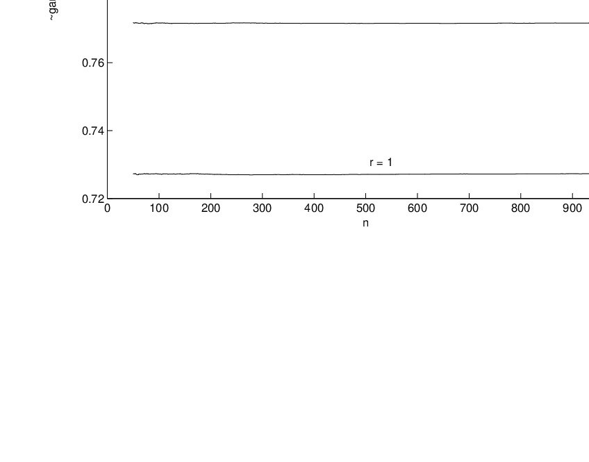
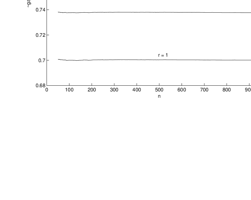
Shown in figure (2) are M​o​n​t​e​C​a​r​l​o​(𝐄𝐋n,2,rB)n\frac{MonteCarlo(\mathbf{EL}_{n,2,r}^{B})}{n} and M​o​n​t​e​C​a​r​l​o​(𝐄𝐋n,2,rB)+Arn\frac{MonteCarlo(\mathbf{EL}_{n,2,r}^{B})\mathbf{+}A_{r}}{n} and the corresponding Random String model data is shown in (3). It appears that the approximation 𝐄𝐋n,2,r\mathbf{EL}_{n,2,r} ∼\mathbf{\sim} γ2,r​n−Ar\gamma_{2,r}n-A_{r} gets increasingly worse for larger rr and likewise for the Bernoulli Matching model.

Refer to caption
Refer to caption
Figure 2: The Monte Carlo approximations of 𝐄𝐋n,2,rBn\frac{\mathbf{EL}_{n,2,r}^{B}}{n} and this same data corrected by (13) to obtain the limiting behavior.
Refer to caption
Refer to caption
Figure 3: The Monte Carlo approximations of 𝐄𝐋n,2,rn\frac{\mathbf{EL}_{n,2,r}}{n} and this same data corrected by (13) to obtain the limiting behavior.

For the Bernoulli Matching model we also can compute 𝐄𝐋n,2,rB\mathbf{EL}_{n,2,r}^{B} exactly for small nn by applying (2) directly beginning with Pr​(z)→\overrightarrow{P_{r}(z)}. This allows us to do two checks on the quality of the Monte Carlo approximations. Firstly, we can observe the difference M​o​n​t​e​C​a​r​l​o​(𝐄𝐋n,2,rB)n−𝐄𝐋n,2,rBn\frac{MonteCarlo(\mathbf{EL}_{n,2,r}^{B})}{n}-\frac{\mathbf{EL}_{n,2,r}^{B}}{n}. The statistic

Sr≡11000​∑j=11000(M​o​n​t​e​C​a​r​l​o​(𝐄𝐋n,2,rB)n−𝐄𝐋n,2,rBn)2S_{r}\equiv\frac{1}{1000}\mathop{\displaystyle\sum}_{j=1}^{1000}\left(\frac{MonteCarlo(\mathbf{EL}_{n,2,r}^{B})}{n}-\frac{\mathbf{EL}_{n,2,r}^{B}}{n}\right)^{2}

gives us an idea of how crude an approximation we get with 1000010000 trials. Also, we can see how good the approximation 𝐄𝐋n,2,rB\mathbf{EL}_{n,2,r}^{B} ∼\mathbf{\sim} γ2,rB​n−ArB\gamma_{2,r}^{B}n-A_{r}^{B} is by using that on the exact values of 𝐄𝐋n,2,rB\mathbf{EL}_{n,2,r}^{B} to extrapolate γ2,rB\gamma_{2,r}^{B} (for this extrapolation we use n=1​…​2000n=1...2000).

rr SrS_{r} Monte Carlo γ2,rB\gamma_{2,r}^{B} γ2,rB\gamma_{2,r}^{B} from 𝐄𝐋n,2,rB\mathbf{EL}_{n,2,r}^{B} γ2,rB\gamma_{2,r}^{B} from fractionsderived previously{\text{from fractions}\atop\text{derived previously}}
11 5.2994×10−85.2994\times 10^{-8} 0.72726340.7272634 0.72727272730.7272727273 0.72727272720.7272727272
22 5.0758×10−85.0758\times 10^{-8} 0.77166760.7716676 0.77157360430.7715736043 0.77157360400.7715736040
33 1.0180×10−81.0180\times 10^{-8} 0.78898740.7889874 0.78896938510.7889693851 0.78896938530.7889693853
44 1.5954×10−81.5954\times 10^{-8} 0.79813540.7981354 0.79822220510.7982222051 −-
rr Monte Carlo ArBA_{r}^{B} ArBA_{r}^{B} from 𝐄𝐋n,2,rB\mathbf{EL}_{n,2,r}^{B} ArB​from fractionsderived previouslyA_{r}^{B}{\text{from fractions}\atop\text{derived previously}}
11 0.27710.2771 0.2644630.264463 0.26446280.2644628
22 0.46260.4626 0.4347450.434745 0.43474450.4347445
33 0.56410.5641 0.5743120.574312 −-
44 0.68520.6852 0.6965340.696534 −-

We also note that M​o​n​t​e​C​a​r​l​o​(γ2,1)=0.7001417MonteCarlo(\gamma_{2,1})=0.7001417 compared to γ2,1=.7\gamma_{2,1}=.7 and M​o​n​t​e​C​a​r​l​o​(A2,1)=0.2652MonteCarlo(A_{2,1})=0.2652 compared to A2,1=.28A_{2,1}=.28

5 Conclusions and future work

It is hoped that the results presented in this paper lead the way to more significant results. In particular, it is hoped that the Random String model analysis may lead to a short proof of γ2,1<γ2,1B\gamma_{2,1}<\gamma_{2,1}^{B}. The limiting behavior of γk,1−γk,1B\gamma_{k,1}-\gamma_{k,1}^{B} would also be of interest. We seek a conjecture for the quantities γk,rB\gamma_{k,r}^{B}, though it is unclear if trying to determine γkB\gamma_{k}^{B} via limr⟶∞γk,rB=γkB\lim_{r\longrightarrow\infty}\gamma_{k,r}^{B}=\gamma_{k}^{B} is a good idea.

The pseudoproof of γkB=21+k\gamma_{k}^{B}=\frac{2}{1+\sqrt{k}} given by Boutet de Monvel may provide a way to simplify the r-reach computations. The limiting behavior of r-reach may be describable only by differences between adjacent values of 𝐑,\mathbf{R,} thereby reducing the ”problemsize” from 22​r2^{2r} to 2​r2r. Preliminary investigations suggest that this reduction may be possible but not as straight forward as the argument in the pseudoproof.

6 Appendix

The expanded version of the Bernoulli Matching model r=1,k=2r=1,k=2 case has matrices as follows. These are given for comparison with the matrices for the Random String model r=1,k=2r=1,k=2 case.

 Pn−1off​(z,z,z)Pn−1off​(z,z,z−1)Pn−1off​(z,z−1,z)Pn−1off​(z,z−1,z−1)Pn−1on​(z,z,z)Pn−1on​(z,z,z−1)Pn−1on​(z,z−1,z)Pn−1on​(z,z−1,z−1)[1/800000001/400000001/400000001/200000001/800000001/400000001/400000001/20000000]=𝐌\text{ \ \ \ \ }\begin{array}[]{l}{\small P}_{n-1}^{\text{off}}{\small(z,z,z)}\\ {\small P}_{n-1}^{\text{off}}{\small(z,z,z-1)}\\ {\small P}_{n-1}^{\text{off}}{\small(z,z-1,z)}\\ {\small P}_{n-1}^{\text{off}}{\small(z,z-1,z-1)}\\ {\small P}_{n-1}^{\text{on}}{\small(z,z,z)}\\ {\small P}_{n-1}^{\text{on}}{\small(z,z,z-1)}\\ {\small P}_{n-1}^{\text{on}}{\small(z,z-1,z)}\\ {\small P}_{n-1}^{\text{on}}{\small(z,z-1,z-1)}\end{array}\begin{bmatrix}{\small 1/8}&{\small 0}&{\small 0}&{\small 0}&{\small 0}&{\small 0}&{\small 0}&{\small 0}\\ {\small 1/4}&{\small 0}&{\small 0}&{\small 0}&{\small 0}&{\small 0}&{\small 0}&{\small 0}\\ {\small 1/4}&{\small 0}&{\small 0}&{\small 0}&{\small 0}&{\small 0}&{\small 0}&{\small 0}\\ {\small 1/2}&{\small 0}&{\small 0}&{\small 0}&{\small 0}&{\small 0}&{\small 0}&{\small 0}\\ {\small 1/8}&{\small 0}&{\small 0}&{\small 0}&{\small 0}&{\small 0}&{\small 0}&{\small 0}\\ {\small 1/4}&{\small 0}&{\small 0}&{\small 0}&{\small 0}&{\small 0}&{\small 0}&{\small 0}\\ {\small 1/4}&{\small 0}&{\small 0}&{\small 0}&{\small 0}&{\small 0}&{\small 0}&{\small 0}\\ {\small 1/2}&{\small 0}&{\small 0}&{\small 0}&{\small 0}&{\small 0}&{\small 0}&{\small 0}\end{bmatrix}=\mathbf{M}
 Pn−1off​(z−1,z−1,z−1)Pn−1off​(z−1,z−1,z−2)Pn−1off​(z−1,z−2,z−1)Pn−1off​(z−1,z−2,z−2)Pn−1on​(z−1,z−1,z−1)Pn−1on​(z−1,z−1,z−2)Pn−1on​(z−1,z−2,z−1)Pn−1on​(z−1,z−2,z−2)[1/81/81/801/81/81/81/801/40001/401/4001/40001/41/400000001/21/81/81/801/81/81/81/801/40001/401/4001/40001/41/400000001/2]=𝐍\text{ \ \ \ \ }\begin{array}[]{l}{\small P}_{n-1}^{\text{off}}{\small(z-1,z-1,z-1)}\\ {\small P}_{n-1}^{\text{off}}{\small(z-1,z-1,z-2)}\\ {\small P}_{n-1}^{\text{off}}{\small(z-1,z-2,z-1)}\\ {\small P}_{n-1}^{\text{off}}{\small(z-1,z-2,z-2)}\\ {\small P}_{n-1}^{\text{on}}{\small(z-1,z-1,z-1)}\\ {\small P}_{n-1}^{\text{on}}{\small(z-1,z-1,z-2)}\\ {\small P}_{n-1}^{\text{on}}{\small(z-1,z-2,z-1)}\\ {\small P}_{n-1}^{\text{on}}{\small(z-1,z-2,z-2)}\end{array}\begin{bmatrix}{\small 1/8}&{\small 1/8}&{\small 1/8}&{\small 0}&{\small 1/8}&{\small 1/8}&{\small 1/8}&{\small 1/8}\\ {\small 0}&{\small 1/4}&{\small 0}&{\small 0}&{\small 0}&{\small 1/4}&{\small 0}&{\small 1/4}\\ {\small 0}&{\small 0}&{\small 1/4}&{\small 0}&{\small 0}&{\small 0}&1{\small/4}&{\small 1/4}\\ {\small 0}&{\small 0}&{\small 0}&{\small 0}&{\small 0}&{\small 0}&{\small 0}&{\small 1/2}\\ {\small 1/8}&{\small 1/8}&{\small 1/8}&{\small 0}&{\small 1/8}&{\small 1/8}&{\small 1/8}&{\small 1/8}\\ {\small 0}&1/4&{\small 0}&{\small 0}&{\small 0}&1/4&{\small 0}&{\small 1/4}\\ {\small 0}&{\small 0}&{\small 1/4}&{\small 0}&{\small 0}&{\small 0}&{\small 1/4}&{\small 1/4}\\ {\small 0}&{\small 0}&{\small 0}&{\small 0}&{\small 0}&{\small 0}&{\small 0}&1/2\end{bmatrix}=\mathbf{N}

References

  • [1] R. A. Baeza-Yates, R. Gavaldà, G. Navarro, and R. Scheihing. Bounding the Expected Length of Longest Common Subsequences and Forests, Theory Comput. Systems 32 (1999), 435-452.
  • [2] Boutet de Monvel, J. Extensive Simulations for Longest Common Subsequences. Europ. Phys. J. B 7 (1999), 293-308.
  • [3] V. Dančík. Expected Length of Longest Common Subsequences. Ph.D. Thesis, CS Dept., University of Warwick, Warwick, England, 1994.
  • [4] D. Sankoff and J. B. Kruskal. Time Warps, String Edits, and Macromolecules: The Theory and Practice of Sequence Comparison, Addison-Wesley, Reading, MA, 1983.
  • [5] Y. Sinai. Probability Theory, Springer-Verlag, Berlin, 1992.