A splitting formula for the spectral flow of the odd signature operator on –manifoldscoupled to a path of connections
Abstract
We establish a splitting formula for the spectral flow of the odd signature operator on a closed –manifold coupled to a path of connections, provided , where is the solid torus. It describes the spectral flow on in terms of the spectral flow on , the spectral flow on (with certain Atiyah–Patodi–Singer boundary conditions), and two correction terms which depend only on the endpoints.
Our result improves on other splitting theorems by removing assumptions on the non-resonance level of the odd signature operator or the dimension of the kernel of the tangential operator, and allows progress towards a conjecture by Lisa Jeffrey in her work on Witten’s –manifold invariants in the context of the asymptotic expansion conjecture [17].
keywords
Spectral flow, odd signature operator, gauge theory, Chern–Simons theory, Atiyah–Patodi–Singer boundary conditions, Maslov indexhttp://www.math.uni-bonn.de/people/himpel/
57M27 \secondaryclass57R57, 53D12, 58J30
eometry & opology Volume 9 (2005) 2261–2302\nlPublished: 6 December 2005
Email:\stdspace\theemail
URL:\stdspace\theurl
Abstract
AMS Classification numbers Primary: \theprimaryclass
Secondary: \thesecondaryclass
Keywords: \thekeywords
Proposed: Ronald Stern Received: 4 December 2004\nlSeconded: Peter Teichner, Ronald Fintushel Accepted: 1 November 2005
1 Introduction
This article analyzes the spectral flow of the odd signature operator coupled to a path of connections on a 3 manifold given a decomposition with a solid torus.
The question is motivated by Edward Witten’s description of certain –manifold invariants [26] and Lisa Jeffrey’s work [17] on the asymptotic expansion conjecture [25, Conjectures 7.6 and 7.7], particularly [17, Conjecture 5.8] in the case of torus bundles over .
This work is preceded by Paul Kirk and Erik Klassen [20] where they treat the problem of computing the spectral flow between irreducible flat connections under some restrictions. In this paper these restrictions are removed.
In particular Kirk and Klassen analyzed the spectral flow on a torus bundle over the circle by way of the splitting theorem in [8] applied to a decomposition of the manifold into a solid torus and its complement. They showed that the spectral flow between irreducible, flat connections is [20, Theorem 7.5], provided that the kernel of the tangential operator for the odd signature operator on the splitting torus along the path of connections has constant dimension.
Kirk and Klassen proposed [20, Appendix] that it might be possible to always to find a solid torus so that the kernel of the tangential operator has constant dimension. It is shown in Proposition 6.2.1, that this is not always the case. Thus we are forced to deal with the case that the dimension changes.
There have been a lot of general splitting formulas [8, 6, 11, 23, 24]. Unfortunately, for all practical purposes one has to make a couple of technical assumptions in order to apply any of these splitting formulas, namely
- 1.
that the non-resonance level (see [24]) of the operator in question is zero, and
- 2.
that the kernel of the tangential operator has constant dimension.
The purpose of this article is to establish a splitting formula in the case where one side is a solid torus without making the above assumptions. We will also show how to apply this tool to explicitly to compute spectral flow.
The main results of this article are the following.
- •
- •
In Section 4 we consider a decomposition of a 3 manifold with the solid torus and express the spectral flow of the twisted odd signature operator between flat connections as the sum of the spectral flow on , the spectral flow on (with boundary conditions ), and two Maslov triple indices (Theorem 4.3.1).
- •
- •
In Section 6 we use Theorem 4.3.1 to compute the spectral flow of the twisted odd signature operator between irreducible, flat connections on torus bundles over (Theorem 6.3.3). In particular we eliminate the technical assumption used in [20] on the dimension of the kernel of the twisted de Rham operator.
Complete calculations and proofs can be found in the author’s thesis [15].
Acknowledgments The results of this article were obtained during the author’s Ph.D. studies at Indiana University, Bloomington. The author is grateful for the guidance and support of his advisor and friend Paul Kirk. The comments of the referee were much appreciated. The author thanks the Max–Planck–Institut in Bonn for their hospitality and financial support while this paper was written.
2 Preliminaries
Familiarity with [3, 20, 23, 24] is useful. However, we introduce all the necessary facts for the convenience of the reader.
2.1 Setup
For the rest of the article let us assume the following.

- 1.
The orientation of the torus is determined by . is given the product metric with the standard metric on . The fundamental group is the free abelian group generated by and .
- 2.
The solid torus is oriented so that is a positive multiple of the volume form when and we have as oriented manifolds (outward normal first convention). Consider a metric on such that a collar of may be isometrically identified with . is equipped with the product metric of our metrics on and . Then there is a collar of which is isometric to . This is consistent with our metric on . The fundamental group is infinite cyclic generated by , and is trivial in .
- 3.
The –manifold has boundary and is oriented so that as oriented manifolds. Consider a metric on such that a collar of is isometric to .
- 4.
- 5.
Let be a trivialized principal bundle with structure group over and consider its restriction to , and .
2.2 Spectral flow
Let , , be a –parameter family of (possibly unbounded) self-adjoint operators with compact resolvent, continuous in the graph metric. Then, given smaller than the modulus of the largest negative eigenvalue of and , the spectral flow is roughly defined to be the algebraic intersection number in of the track of the spectrum
and the line segment from to . The orientations are chosen so that if has spectrum then . For a detailed discussion on spectral flow with rigorous definitions and proofs see [4].
Given a continuous family of self-adjoint elliptic operators on a closed manifold , one can use standard theorems (for example in [18]) to conclude that the spectrum is discrete for each and varies continuously in .
For a compact manifold with boundary one needs to choose boundary conditions. In [4] the authors treat this in more generality, but for the results in the present article it is sufficient to confine ourselves to Atiyah–Patodi–Singer boundary conditions (see Section 2.5 for a definition) on a manifold with a collar. It is shown in [21], that by choosing a continuous family of Atiyah–Patodi–Singer boundary conditions the spectrum of varies continuously in (see [21, Theorem 4.1 and Section 5]).
2.3 Connections and representations
There are several equivalent definitions for connections, but in the case of principal bundles over –manifolds we have a particularly nice description for connections.
We will identify the Lie group with the unit quaternions
The group multiplication will be the usual multiplication in the quaternions. Its Lie algebra can be identified with the vector space of imaginary quaternions. The adjoint action ad of on corresponds to the conjugation of imaginary quaternions by unit quaternions.
Consider the principal bundle over . The chosen trivialization of induces an identification
- •
of the group of gauge transformations with , and
- •
of the affine space of connections with Lie-algebra-valued –forms on , where the product (or trivial) connection corresponds to .
Then the action of a gauge transformation on an connection on is given by
The choice of trivialization induces a trivialization of the adjoint bundle associated to . Thus we can associate to a connection on a covariant derivative on by defining
where means taking the Lie bracket on the coefficients and wedging the form part. We extend the covariant derivative to by the Leibniz rule.
The curvature of a connection is the –form in defined by , where . We have . We call flat, if . Let be the set of all flat connections on . If is flat, then the holonomy is a representation of the fundamental group of .
Let be the set of conjugacy classes of representations of the fundamental group . Then the holonomy map identifies with [13, Proposition 2.2.3].
2.4 The odd signature operator and the de Rham operator
We introduce two first order differential operators on and . These depend on the orientation and the Riemannian metric on and , which we fixed in Section 2.1. We set , .
The inner product on and is given in terms of the Hodge operator by
For an connection the odd signature operator twisted by is defined to be
For an connection de Rham operator twisted by is defined to be
In fact, is the tangential operator of (see [3, Lemma 2.4]). and are first-order self-adjoint elliptic differential operator.
The following important and well-known fact is an application of the Atiyah–Patodi–Singer index theorem (compare with [22, Theorem 7.1]):
Proposition 2.4.1.
Suppose is a closed –manifold and is a gauge transformation. If is any path of connections on from to , then
2.5 Eigenspaces of the de Rham operator
Let and . Denote by the –eigenspace of and let
Abbreviate . By the spectral theorem for self-adjoint elliptic operators we have
We define an almost complex structure on by
One can see that and that is an isometry of . The induced symplectic structure is compatible with , which makes into a symplectic space with compatible almost complex structure. A subspace of is Lagrangian if .
is a finite dimensional symplectic subspace of . Furthermore, if is a Lagrangian subspace of , then is Lagrangian in .
A Lagrangian subspace is called an Atiyah–Patodi–Singer (APS) boundary condition, if contains all eigenvectors of the tangential operator with sufficiently large eigenvalues.
Let be the Laplacian on twisted by . Denote the harmonic , and –forms of and by and respectively.
If is flat, we have and consequently . Thus a –eigenvector of is a –eigenvector of . Furthermore, a direct computation shows the following.
Lemma 2.5.1.
If is flat and is a –eigenvector () for , then is a –eigenvector for . Furthermore .
2.6 Cauchy data spaces and adiabatic limits
Cauchy data spaces play an important role in this work because of their relation to spectral flow. Liviu Nicolaescu analyzed this relationship in [24]. His results have been extended by [11] and [23]. The facts in this section make up the main tools for this work.
We will state all results in this section in terms of the odd signature operator on , but they apply to other self-adjoint Dirac type operators as well.
We introduce the notation
| and | ||||
| and |
for .
Let be a connection on , which is in cylindrical form in a collar of , that is , where is the inclusion at and .
We write the restriction of to as
where denotes contraction of with , and is the Hodge star on differential forms on the –manifold . This also gives us a restriction map of and to . If we write , where is the coordinate in and does not have a component, then a more intuitive way to write the restriction map is .
The Cauchy data space of is
and the scattering Lagrangian or the limiting values of extended solutions is
See [2] for more information on Cauchy data spaces, particularly [2, Definition 2.22]. Note that we can extend to and that is a continuous family of Lagrangian subspaces by [11, Lemma 3.2]. Denote .
For flat the kernel of is isomorphic to the cohomology with values in twisted by via the Hodge and de Rham theorems. See for example [12, Chapter 5] for a definition of the cohomology of twisted by a representation .
The following gives a way to compute the scattering Lagrangian at a flat connection.
Proposition 2.6.1 (Corollary 8.4, [23]).
If is flat on , then is isomorphic to via the Hodge and de Rham theorems.
Cauchy data spaces are complicated and we wish to relate them to simpler Lagrangians. The situation is particularly favorable when has non-resonance level . Nicolaescu [24] defines to have non-resonance level , if .
Nicolaescu’s adiabatic limit theorem describes the limit of the Cauchy data spaces of under stretching the collar.
Theorem 2.6.2 (Corollary 4.11, [24]).
If has non-resonance level , then
We will need some facts about the non-resonance level situation. In analogy to [3, Proposition 2.10] we have the following from [1, Proposition 4.9].
Proposition 2.6.3.
Let be flat.
- 1.
We have
Thus non-resonance level is equivalent to
- 2.
Assuming non-resonance level, we get the isomorphism
Kirk and Lesch [23] give a detailed decomposition of in the spirit of the Hodge decomposition as an orthogonal sum of symplectic spaces
| (2.6.1) |
When is flat, we do not only get an explicit description of the scattering Lagrangian (Proposition 2.6.1), but the adiabatic limit has a nice description when the the non-resonance level is not .
Theorem 2.6.4 (Theorem 8.5, [23]).
If is flat, then there exists a subspace
isomorphic to
so that if denotes the orthogonal complement of in , then with respect to the decomposition (2.6.1) into symplectic subspaces, the adiabatic limit of the Cauchy data spaces decomposes as a direct sum of Lagrangian subspaces:
where denotes the scattering Lagrangian on .
In due course, we will need to have control over the intersection of the Cauchy data spaces with other Lagrangian subspaces when we stretch the collar. Thus the following results are important.
Proposition 2.6.5 (Lemma 8.10, [23]).
Let be flat, and consider a Lagrangian subspace .
- 1.
The dimension of is independent of .
- 2.
The dimension of is independent of .
- 3.
The dimension of is independent of .
2.7 Maslov index
Let be a symplectic Hilbert space with compatible almost complex structure . A pair of Lagrangians in is called Fredholm if is closed and both and are finite. Consider a continuous path of Fredholm pairs of Lagrangians in . Continuity is measured in the gap topology. If and are transverse at the end points, that is, intersect trivially, then the Maslov index is roughly defined to be a count of how many times and intersect with sign and multiplicity, that is, counting the dimension of the intersection. For a careful definition see [7, 24, 9]. If the intersection of and is nontrivial at the endpoints, we will choose a convention compatible with our spectral flow convention (in view of Theorem 2.7.1): Given a continuous –parameter family of Fredholm pairs of Lagrangians , , choose small enough so that
- 1.
is transverse to for and , and
- 2.
is a Fredholm pair for all and all .
Then the Maslov index of the pair is the Maslov index of .
A splitting theorem for spectral flow by Nicolaescu [24] in terms of a Maslov index has been extended in [10] to the situation when the Dirac operators are not invertible at the endpoints. Also see [23, Theorem 7.6] for a proof of the same result. The precise statement in the context of the odd signature operator and connections on is the following.
Theorem 2.7.1 (Theorem 4.3, [10]).
Suppose is a continuous path of connections on in cylindrical form in a collar of . Then the path consists of Fredholm pairs of Lagrangians and
We also have a relative version of this theorem (see [9] and [24]) which relates spectral flow on a manifold with boundary with APS boundary conditions to some Maslov index. It is implied by the results in [10].
Theorem 2.7.2.
If is a path of connections on in cylindrical form near and is a continuous family of self-adjoint APS boundary conditions, then the spectral flow is well defined and .
We will also use a Maslov triple index as defined in [23], which is up to normalization the same as Bunke’s Maslov triple index in [6] and different from the Maslov triple index usually considered in the literature (see [7]). In our notation, we define it for triples of Lagrangian subspaces of a symplectic Hilbert space with almost complex structure , such that is a Fredholm pair for all . We set for some Lagrangian subspace and use [23, Formula (6.21)] to define for other triples: If , and , are paths of Lagrangian subspaces, such that is a Fredholm pair for all , , then the (twisted) Maslov triple index is determined by requiring that
The indices and share some properties. For example is additive under direct sums (symplectic additivity). Furthermore the following properties are an elementary consequence of the above characterization, and can also be found in [23, Proposition 6.11].
Lemma 2.7.3.
Let , be pairwise Fredholm Lagrangians in a Hilbertspace . Then
- •
, and
- •
.
- •
.
3 A family of Atiyah–Patodi–Singer boundary conditions
This section introduces a specific family of Atiyah–Patodi–Singer boundary conditions for the odd signature operator on a manifold with torus boundary.
The results will be used for the analysis of the spectral flow for the splitting in Section 4, where is the solid torus. In Section, 5 we will explicitly compute spectral flow on with the boundary conditions developed in this section.
3.1 A family of flat connections on the torus
Let be the set of conjugacy classes of representations of the fundamental group of .
The holonomy map gives a homeomorphism from the gauge equivalence classes of the flat connections on to [13, Proposition 2.2.3]. If with , then is given in quaternionic notation by
| (3.1.1) |
Notice, that is a branched cover of , with branch points the half integer lattice, which map to central representations, and covering transformations , . Each then also corresponds to an connection on . Thus, We have a smooth family of flat connections with holonomy as in (3.1.1) parametrized by , which projects onto .
Definition 3.1.1.
Let . We substitute an index by , for example and .
The harmonic forms of are equal to the kernel of by Lemma 2.5.1. By we denote the –linear combinations of the function . The following straightforward computation of the harmonic forms on the torus is left to the reader.
Proposition 3.1.2.
Also observe that preserves the and –part of , and we can write
as well as
3.2 Boundary conditions
We want a path of self-adjoint operators which is continuous in the graph topology. In order for the odd signature operator on or to vary continuously and be (unbounded) self-adjoint, we need a path of boundary conditions which is continuous in the gap topology. See [4] for details.
We might like to pick a continuous family of Lagrangians in and extend it to a family of APS boundary conditions in by or . Unfortunately, not only does the dimension of the kernel of the tangential operator jump up at (see Proposition 3.1.2), but for a smooth path , , through we have
In fact the part of the limits turn out to be orthogonal to each other.
Thus we introduce the space shown in Figure 2 to parametrize the Lagrangians. It is with open disks of radius removed around all half integer lattice points with the induced topology. Some people would call it the real blow-up of the plane at the half integer lattice points. We will see in Theorem 3.2.2, why this is a good parameter space. The advantage of this space is that we can easily homotop paths of connections together with their boundary conditions, thus getting a homotopy of paths of self-adjoint operators. However, it will be more convenient to parametrize by the following space.

Definition 3.2.1.
Let , where if . We will simply write . Alternatively it is convenient to think of elements in as being of the form
Denote by the projection . Let us define a bijection between and .
We will describe what this bijection looks like around the origin. At all the other half integer lattice points we get a similar bijection via translation. Away from disks of radius around each half integer lattice point the bijection is the identity map. Identify with in the usual way. Let be the disk of radius , and the disk of radius with an open disk of radius around the origin removed, that is, an annulus. Let be a smooth (cutoff) function with
Then the bijection is given by . We give the topology that makes the bijection into a homeomorphism. Notice that is a diffeomorphism away from .
Theorem 3.2.2.
Let and . Then
- 1.
is continuous.
- 2.
Moreover exists and we can define
Note that for .
- 3.
is continuous.
- 4.
If , then
where and
Notice from the explicit description of that . Before we prove this theorem, an eigenspace decomposition will be useful to compute explicitly and study the behaviour of the family around the half integer lattice. It is a lengthy but straightforward computation, which we will leave to the reader.
Proposition 3.2.3.
Fix . We have the orthogonal decomposition
where forms in
are eigenvectors of with eigenvalue , and forms in
are eigenvectors of with eigenvalue . and are the harmonic forms of the untwisted Laplacian.
Proof of Theorem 3.2.2.
For the continuity of away from see [21]. We show that exists by explicitly computing for .
Let , . By Proposition 3.2.3 is an eigenvector of with eigenvalue . Then by Lemma 2.5.1
is a –eigenvector of . This yields
For we similarly get
Repeating the same computation for and yields a total of linearly independent eigenvectors, which lie in either or . By Proposition 3.1.2 the part of is –dimensional. Thus the –span of the above eigenvectors make up or . This completes the computation of and shows that exists.
We are left with proving the continuity of parametrized by . Away from the family is continuous since . To show continuity at half integer lattice points, it suffices to show that for any continuous path in that limits to we have
For all other half integer lattice points the argument is the same. By definition is continuous in a ball of radius around , if is continuous in , where is the homeomorphism given in Definition 3.2.1. We consider two cases:
- 1.
If for small, then and continuous for small . Elementary triangle equality arguments applied to , small, show that is continuous.
- 2.
Thus is a continuous family parametrized by . ∎
Definition 3.2.4.
For a continuous family of Lagrangians of parametrized by a subset , define a family of subspaces of parametrized by as follows
For our application, the family of Lagrangians will be independent of . Notice that vanishes away from , while we have “blown up” the points of and removed the singularities that paths through encounter. Here is a corollary of Theorem 3.2.2, which is important for the following sections.
Theorem 3.2.5.
is a continuous family of Lagrangians parametrized by .
4 Spectral flow on a closed –manifold
In this section we develop a splitting formula for spectral flow, which expresses spectral flow of the odd signature operator between flat connections on a closed –manifold in terms of spectral flow on the solid torus and its complement with the Atiyah–Patodi–Singer boundary conditions from Section 3. Even though Nicolaescu [24] and Daniel [10] provide us by way of Theorem 2.7.1 with an elegant expression of spectral flow in terms of the Maslov index of the respective Cauchy data spaces, it is not immediately applicable to spectral flow computations, since the Cauchy data spaces themselves are complicated objects. The purpose of the splitting formula in Theorem 4.3.1, however, is to make computations of spectral flow easier by shifting the problem to two more tractable ones. In fact, an explicit way to compute the spectral flow on is given in Theorem 5.3.3. One only needs to do some work computing the spectral flow on . The main application to keep in mind is the spectral flow computation of the twisted odd signature operator between flat connections, whenever it is possible to find a path between them which is flat on , because then we can use topology to try computing the spectral flow on .
4.1 Objective
The setup in this section is as follows. Let be a closed –manifold with being the solid torus and the torus as in Section 2.1. Let be a path of connections on with the following properties:
- 1.
is in cylindrical form and flat in a collar of .
- 2.
restricts to the path (see Definition 3.1.1) on for some path in with , where is the projection onto the –factor.
- 3.
and are flat on .
The goal in this section is to find a splitting formula expressing in terms of spectral flow on and . Notice that, while the spectral flow on and depends on the lift of in property (2), and are independent of it.
The above assumptions do not limit the applicability of the splitting formula in Theorem 4.3.1. Indeed, the spectral flow of the odd signature operator along a path of connections with flat endpoints depends only on and , which we can gauge transform by some , so that . The change in spectral flow is given by Proposition 2.4.1. We can extend the path by obstruction theory to a path of connections on with endpoints and , since is contractible.
4.2 The scattering Lagrangian of on
Before we start with the discussion of the spectral flow on , we analyze the scattering Lagrangian of at a flat connection on which restricts to on , because its explicit description plays a central role in the splitting theorem.
The scattering Lagrangian of for can be computed directly.
Consider a flat connection on with . One observes that is a surjection and . Thus we have , that is, , and in view of Proposition 2.6.1 the scattering Lagrangian depends only on . Therefore we can use a gauge transformation with on the boundary to compute . This yields the following.
Lemma 4.2.1.
Suppose is a flat connection on with . Then and
- •
for ,
- •
for , where
Thus we make the following definition.
Definition 4.2.2.
For define . Note that .
4.3 A splitting formula for spectral flow
We will derive the following splitting formula.
Theorem 4.3.1.
Let be a closed –manifold with being the solid torus and the torus as in Section 2.1. Let be a path of connections on with the following properties:
- 1.
is in cylindrical form and flat in a collar of .
- 2.
restricts to the path on for some path in with , where is the projection onto the –factor.
- 3.
and are flat on .
Then we have the splitting formula:
The proof of Theorem 4.3.1 is deferred to the next section. However, the idea is the following. First we relate the spectral flow to the Maslov index of the Cauchy data spaces using Nicolaescu’s splitting theorem. Next we use homotopy invariance of the Maslov index and Nicolaescu’s adiabatic limit theorem to find homotopic paths of Lagrangians, parts of which correspond to a Maslov index of Cauchy data space with APS boundary conditions. Now we can use additivity of pairs of paths of Lagrangians and apply the relative version of Nicolaescu’s splitting theorem to two of the parts, which yields the first two summands of the formula. The remaining summands will either vanish or simplify to the two Maslov triple indices involving from Theorem 3.2.2, the scattering Lagrangians and at , as well as from Lemma 4.2.1.
The situation is particularly nice and straightforward when
- 1.
and restricted to have non-resonance level , and
- 2.
for all , in which case .
We describe the derivation of our splitting formula without these assumptions.
Fix the path which corresponds to the parameter that stretches the collar from to . Stretching the collar of yields the adiabatic limit , because has non-resonance level when . Theorem 2.6.4 describes .
Since for (see Theorem 3.2.2), we will use the APS boundary conditions and for our splitting formula with the notation introduced in Definition 3.2.4 and Lemma 4.2.1, which were shown to be continuous for a continuous lift of the path from to .
We will need to “rotate” the adiabatic limit of and to our preferred APS boundary conditions.
Definition 4.3.2.
We introduce the paths for and for as follows:
- 1.
Let be a path of Lagrangians in from the scattering Lagrangian to .
- 2.
is a path of Lagrangians in from to .
- 3.
For let be a path of Lagrangians in , where is an arbitrary path from to . As in Lemma 4.2.1, denotes the part of . Set .
Then it is straightforward to check that the composition of paths given in Table 1 is homotopic to the path of pairs of Cauchy data spaces . The table shows the –th paths and in the second and fifth column. The third and fourth column give the endpoints of and as a reference.
If for , then we have , thus
This yields the following.
Corollary 4.3.3.
We make the same assumptions as in Theorem 4.3.1. Then, if for we get:
4.4 Proof of Theorem 4.3.1
By Lemma 2.6.5 the Maslov indices vanish for . By Theorem 2.7.2 we have
Since for all , the Maslov index vanishes. Again by Theorem 2.7.2 we have
Let us focus our attention on the rest of the paths, namely paths 2, 5, 7 and 10.
We may homotop to the composition of the two paths
and to the composition of the two paths
By Lemma 2.6.5 . Then by our choice of we get
We can directly check:
Then Lemma 2.7.3 and linearity under the direct sum of triples yield
We get a similar expression for the paths 5 and 10. The path can be homotoped to the composition of the two paths
and to the composition of the two paths
Again by Lemma 2.6.5 we get . Thus
while
Thus
Notice that since and are both homotopic to constant paths, we can compute
Just like for the paths 2 and 7 this simplifies to
This shows that simplifies to the desired formula and completes the proof.∎
5 Spectral flow on the solid torus
In our main application discussed in Section 6 we are interested in computing spectral flow of the twisted odd signature operator along a path of connections on torus bundles over . The main tool is our splitting formula for spectral flow from Theorem 4.3.1, by which we ultimately need to compute spectral flow on a solid torus and on its complement with certain APS boundary conditions.
While the spectral flow computation on certainly depends on itself, we will discuss spectral flow on separately, as it might be interesting and applicable in other settings.
5.1 Objective
Let be the solid torus and its boundary. Let be the family of connections on as described in Definition 5.2.1 and let be a path of connections on the solid torus , so that and are flat connections. Boundary conditions are necessary to make the odd signature on (unbounded) self-adjoint. The Atiyah–Patodi–Singer (APS) boundary conditions discussed in Section 3 are suitable for our purpose. The goal is to compute the spectral flow of on , where .
Since with covers all gauge equivalence classes of flat connections on , the restriction to a path in is suitable for its use in a splitting formula, as we discussed in Section 4.1.
5.2 A smooth family of connections on parametrized by
We would like to extend the family of flat connections on given in Definition 3.1.1 to a family (smoothly parametrized by ) of connections on , so that
- 1.
is flat for ,
- 2.
the restriction of to a collar of in is .
Notice that makes sense globally as a (flat) connection on for all , whereas does not for . Thus we can try to construct the family, so that
- (3)
is equal to for and .
Since , we can find a gauge transformation on , such that in the collar of
The gauge transformation can easily be constructed factoring through . It will be convenient to fix for a smooth non-decreasing cutoff function with for near and . Since
we get a smooth family of connections on , , with the desired property
This can be easily extended to a smooth family of connections parametrized by with . One possible way is the following:
Definition 5.2.1.
Let be a smooth cutoff function with for and near the core of , which may as well factor through . Let be a partition of unity subordinate to . For define the family
Notice that is an connection on (in normal form) for and . Thus is a smooth family of connections on . It is easy to check, that this family has the following properties:
- 1.
.
- 2.
- 3.
for , which is flat.
5.3 Computation of spectral flow on the solid torus
In this section all connections and odd signature operators are considered on the solid torus only. Everything that follows depends on a continuous family of Lagrangians in parametrized by .
To avoid technical difficulties we are going to assume that is a family of Lagrangians in , which is transverse to (see Definition 4.2.2) for all . Later we will fix a specific family of Lagrangians in view of the splitting formula in Theorem 4.3.1.
Definition 5.3.1.
Define as a function of paths in , where is the projection mentioned in Definition 3.2.1.
Observe that SF is additive under compositions of paths in and that SF is a homotopy invariant rel endpoints.
Lemma 5.3.2.
There is a cohomology class , such that for a path in that starts and ends in the (mod 0) spectral flow equals , where . Note, that corresponds to the thickened vertical lines in Figure 3.

Proof.
By defining for singular –simplices and integers , we get a map .
Now suppose . Then is a path of flat connections on . We have
Then Proposition 2.6.3 and imply that (with boundary conditions ) has no kernel. Furthermore by comparing Theorem 3.2.2 and Lemma 4.2.1 we see that when . This implies that .
Thus descends to a map , that is .
It is straightforward to show using the homotopy invariance and the additivity of SF that is a cocycle. We also observe that by definition a coboundary in vanishes on paths in with endpoints in . Thus we have found the desired cohomology class . ∎
Equivalently we may say (by Poincaré duality) that there exists an infinite homology class in , such that the intersection number with (the homology class representing) the path is equal to the spectral flow.
Fix . Our goal is to compute the (infinite) cycle corresponding to the cohomology class in Lemma 5.3.2, therefore extending [20, Theorem 6.4].
Theorem 5.3.3.
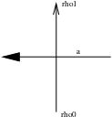
If starts and ends in , then is given by the intersection number where is the cycle shown in Figure 3.
The sign convention for computing the intersection number is determined by the example in Figure 4.
The lengthy proof of Theorem 5.3.3 is deferred to the next section. However, here is a short outline of the proof. Consider a path of connections between flat connections on a certain closed manifold , which restricts to a path in our family of connections on defined in Definition 5.2.1 and lifts to a path in . An example of such a path is shown in Figure 6. Now consider a particular gauge transformation on . Suppose that and . Then we are going to compare the spectral flow of with the spectral flow of given by
using some properties of a particular family of gauge transformations as well as Proposition 2.4.1.
By repeating the above process a few times and applying the splitting formula for spectral flow in Theorem 4.3.1 for different paths we will learn how the chains of the desired (infinite) cycle relate to each other, because the terms of the spectral flow on cancel. This yields the cycle with three unknowns , and . The coefficients in Figure 3 can then be computed using some lens space examples and by applying the splitting formula for spectral flow in Theorem 4.3.1 once more.
Before we embark on a proof of Theorem 5.3.3 we adapt some of the definitions and results in [3] to our needs.
Consider the following group of gauge transformations:
We have by the long exact sequence of the pair , and for . Thus there is a well-defined degree for maps , particularly for elements of .
Lemma 5.3.4 (Lemma 4.1, [3]).
Let . Then and are homotopic if and only if and .
Consider the following gauge transformations on :
- 1.
from Section 5.2,
- 2.
,
- 3.
is a gauge transformation of degree with .
The exact description of these gauge transformations is not relevant for us. However, we will need to exploit some of their properties.
Theorem 5.3.5 (Lemma 4.3, Theorem 4.4, [3]).
We have up to homotopy and
We are going to use one additional gauge transformation on . We set . Notice, that even though , we have for all . Furthermore the following observation is noteworthy because we will need it later.
Lemma 5.3.6.
.
Proof.
We have for by the long exact sequence of the pair . Thus, if a map with misses a point , then it is a composition of maps
and therefore by functoriality of .
Since is homotopic to , we have for any
which implies . ∎
The following useful fact follows immediately from the relative Mayer–Vietoris sequence and the long exact sequence of the pairs and .
Lemma 5.3.7.
Let . If with , then .
We want to close this section with a straightforward Maslov index computation (like the one in the proof of Lemma 6.3.1).
Lemma 5.3.8.
Let . Then for small enough and varying we have
5.4 Proof of Theorem 5.3.3
For simplicity consider the lens space , where
Then we have a family flat connections on which restricts to noncentral connections on . Figure 5 shows which flat connections of the family of connections on extend to flat connections on and . The intersection of the lines corresponding to these flat connections on correspond to flat connections on .

Since , there is no obstruction of extending any to . Denote the extensions of , and by , and respectively. We can simply extend to .
Let be a (straight line) path in which starts at and ends at as shown in Figure 6. Now let be a fixed but arbitrary path of connections on , which is flat at the endpoints and equals for when restricted to as in Definition 5.2.1. Consider the gauge transformation . Define a path of connections on by
| (5.4.1) |
where and . Notice that .

Let . If is a path of APS boundary conditions on let . Occasionally we will also write instead of to emphasize that spectral flow on only depends on the endpoints. Let us compare with by utilizing Proposition 2.4.1. By Definition 5.2.1 we have
and
Notice that . Consider the gauge transformation
By exploiting the homotopy invariance and the additivity of the spectral flow, Proposition 2.4.1 as well as Lemmas 5.3.7 and 5.3.6 (in this order) we get
Let us now apply the splitting formula in Corollary 4.3.3 to both sides of the equation and observe that for a path of connections , a gauge transformation and a path of APS boundary conditions we have
In particular and imply
Thus the spectral flow terms for vanish, and in Figure 6 because of


Now let and consider the straight line path which starts at and ends at , as shown in Figure 8. As before, let be a fixed but arbitrary path of connections on , which equals for when restricted to as in definition 5.2.1. Consider the gauge transformation . Using this data, define a path of connections on as in (5.4.1), where and . Notice that .
Similarly if for the same path we consider , , the gauge transformation , and we define as in (5.4.1), then we have and thus .
A similar computation gives us the relationship between coefficients for the horizontal simplices. Let be a path going half around the origin as shown in Figure 8, for example . Consider and . Let and define as in (5.4.1). Since , we immediately get . The Corollary 4.3.3 yields in Figure 8. Similarly, if or we have , and we get in Figure 8.
Thus we are left with determining the coefficients , and in our cycle in Figure 9.

To find the values of and we refer to Lemma 5.3.8. For we consider the –sphere constructed by gluing two solid tori and with the same orientation along the boundary using the orientation reversing homeomorphism on the boundary . For we get a similar statement as in Lemma 5.3.8. Then we can employ the splitting formula in Theorem 4.3.1 for some paths and with
- •
,
- •
for ,
- •
and constant for .
This yields
and shows that has to equal .∎
6 Spectral flow on a torus bundle over the circle
We are interested in computing the spectral flow of the odd signature operator coupled to a path of connections on a torus bundle over , because it addresses [17, Conjecture 5.8], the missing piece in her work on Witten’s –manifold invariants [17].
Jeffrey considered a mapping torus over the torus and assumed that its monodromy matrix has . Her conjecture, based on physical reasoning, implies that the spectral flow of the odd signature operator between irreducible flat connections is , which shall be confirmed in this section.
Lisa Jeffrey’s conjecture for the case needs some interpretation when the trace of the monodromy matrix is zero as well as when one considers representations of whose restriction to is central (this is equivalent to the condition in the footnote to [17, Conjecture 5.8] for ). Thus we are not able to give a detailed analysis of Lisa Jeffrey’s conjecture in this work. However, it will be the subject of future research.
6.1 Irreducible representations of
Fix an orientation for . Let be an orientation preserving homeomorphism, be its mapping torus and fix a base point in . Consider the isomorphism induced by on homology, and fix a meridian and longitude for so that and so that is in the orientation class, when we consider . After identifying and we can write as an unimodular matrix. If and , then the monodromy matrix is
We will henceforth assume that . This is equivalent to and implies and .
The fundamental group of is an HNN extension of , where is the loop from to :
Recall that we have the identification of with the unit quaternions.
Let . [20, Proposition 5.5] states that the homomorphism
| (6.1.1) |
factors through if and only if . Observe that a representation is reducible if and only if . Furthermore representations and are conjugate if and only if for some . Together with [20, Corollary 7.2] this implies the following.
Lemma 6.1.1.
Any two irreducible representations and of are conjugate to and respectively so that as in (6.1.1) is a path of irreducible representations of
where is a tubular neighborhood of the curve on and is a relatively prime pair satisfying
| (6.1.2) |
Let the longitude be the curve on parallel to and the meridian the curve that bounds a disk in . It is not hard to see that that and are words representing the meridian and longitude. See [20, Figure 3]. Then for we have
where and . Thus a representation of restricts to a central representation on the boundary if and only if and .
6.2 An example
It is conjectured by Kirk and Klassen in [20], that one can always find some and so that the entire path is noncentral when restricted to . The following example shows that this is false. While Kirk and Klassen’s work does not apply here, the present paper does apply to compute the spectral flow.
Consider . Since , conjugacy classes of representations of are uniquely represented by all with for which . There are only two conjugacy classes of irreducible representations. They are represented by and for and .
Any for determines a representation of , where is such that is a relatively prime pair satisfying equation (6.1.2). In this case we have and . Thus we can choose . Conjugates and of and give us a different . For example if we choose and , then .
Proposition 6.2.1.
Let , and . Let and for and a knot satisfying 6.1.2 for and . Then both and are central when restricted to .
Proof.
We have and . Furthermore for we get . Similarly . It follows that is a pair of odd integers. Since are required to be relatively prime, one of them must be odd. Since , both and must be odd. This implies that and are half integers. Since and are also integers, and are central. ∎
A similar example is given by with ,
In addition to the above examples there are also paths with representations in the interior which are central on . The example
are particularly interesting, because all conjugate choices of and seem to still have representations in the interior which are central on the boundary, though no proof has been found.
6.3 Computation of the spectral flow
We compute the mod 4 spectral flow of the odd signature operator on coupled to a path of connections , where and are flat and irreducible. We want to apply the splitting formula in Theorem 4.3.1. By Lemma 6.1.1 we may assume that and , and that with for is a path of irreducible representations of for some curve . The holonomy maps flat connections on to representations of . By [14, Theorem 4.1] there is local splitting of this holonomy map. Thus lifts to a path of irreducible connections on with holonomy , which extends to a path of connections on all of via the family of connections on given in Definition 5.2.1. Notice that where . The slope of corresponds to .
Kirk and Klassen computed the spectral flow of mod 4 [20, Theorem 7.5], when the representations are noncentral for all when restricted to . Recall that is central if and only if .
Let us reparametrize , so that lifts to a path in . The spectral flow on the solid torus in Theorem 4.3.1 has been computed in Theorem 5.3.3. Therefore, we focus on the spectral flow on and the Maslov triple indices in Theorem 4.3.1.
We apply Proposition 2.6.1 to the cohomology computations in [20, Lemma 7.7] to compute the scattering Lagrangian of on when is noncentral. Analogous computations yield when is central but is irreducible. We see that the scattering Lagrangian on splits into the and part , just like the scattering Lagrangian on . We have
and
Thus, by the additivity of the Maslov triple index, the Maslov triple indices in Theorem 4.3.1 reduce to and .
Lemma 6.3.1.
If for some , then for small enough and varying we have
Proof.
By Theorem 3.2.2 we observe
Consider the case . To make notation simpler assume . Then . Notice that and intersect in
Consider the constant path and the path
of –dimensional Lagrangians in the symplectic subspace
parametrized by . These intersect at in . We compute
where denotes composition of paths, and the paths
are parametrized by . Observe that since .
Now for the orthogonal complement in we have
Thus
A similar computation proves the case . ∎
This implies together with Lemma 5.3.8 and the fact that , that the Maslov triple indices are either or each.
Now we analyze the spectral flow on , when passes through the half integer lattice. In the following proposition we compute the spectral flow for its lift in locally around the half integer lattice.
Proposition 6.3.2.
Let be a maximal interval with . Then for small enough and varying the spectral flow
is twice the algebraic intersection number of with .
Proof.
Consider . The computation is the same as in the proof of [20, Lemma 7.7]. For we have by our computation of , Proposition 2.6.1 and the long exact sequence of of the pair that . Together with the computations from [20, Lemma 7.7] we get
Then by Proposition 2.6.3 has non-resonance level 0 on when or .
Recall that by we have and . Thus is transverse to for all and , because the –forms of make up the tangent space to the path by [20, Lemma 6.3].
We have and . Since , we can find an with for . Then has non-resonance level 0, and by Proposition 2.6.3 we get for
For and we also have non-resonance level 0. Since we get
This implies that for and the spectral flow on vanishes.
Since we have non-resonance level on for all we have . By Proposition 2.6.5 and since the Maslov index is invariant under a homotopy of paths of Lagragians which preserves the dimension of the intersections at the endpoints, we get for varying
The first and last summand vanish, the second is determined by Lemma 6.3.1. This completes the computation. ∎
The above proposition together with the computation in the proof of [20, Lemma 7.7], that the spectral flow on picks up 2 mod 4, whenever and , implies that
is a multiple of 4. We summarize.
Theorem 6.3.3.
Let be a path of connections on a torus bundle over , where and are flat and irreducible. Then .
References
- [1] M F Atiyah, V K Patodi, I M Singer, Spectral asymmetry and Riemannian geometry. I, Math. Proc. Cambridge Philos. Soc. 77 (1975) 43–69 \MR0397797
- [2] D Bleecker, B Booss-Bavnbek, Spectral invariants of operators of Dirac type on partitioned manifolds, from: “Aspects of boundary problems in analysis and geometry”, Oper. Theory Adv. Appl. 151, Birkhäuser, Basel (2004) 1–130 \MR2072498
- [3] H U Boden, C M Herald, P A Kirk, E P Klassen, Gauge theoretic invariants of Dehn surgeries on knots, \gtref520016143226 \MR1825661
- [4] B Booss-Bavnbek, M Lesch, J Phillips, Unbounded Fredholm operators and spectral flow, Canad. J. Math. 57 (2005) 225–250 \MR2124916
- [5] B Booß-Bavnbek, K P Wojciechowski, Elliptic boundary problems for Dirac operators, Mathematics: Theory & Applications, Birkhäuser Boston Inc. Boston, MA (1993) \MR1233386
- [6] U Bunke, On the gluing problem for the -invariant, J. Differential Geom. 41 (1995) 397–448 \MR1331973
- [7] S E Cappell, R Lee, E Y Miller, On the Maslov index, Comm. Pure Appl. Math. 47 (1994) 121–186 \MR1263126
- [8] S E Cappell, R Lee, E Y Miller, Self-adjoint elliptic operators and manifold decompositions. I. Low eigenmodes and stretching, Comm. Pure Appl. Math. 49 (1996) 825–866 \MR1391757
- [9] A M Daniel Maslov index, symplectic reduction in a symplectic Hilbert space and a splitting formula for spectral flow, PhD thesis, Indiana University, Bloomington, (1997)
- [10] M Daniel, An extension of a theorem of Nicolaescu on spectral flow and the Maslov index, Proc. Amer. Math. Soc. 128 (2000) 611–619 \MR1622789
- [11] M Daniel, P Kirk, A general splitting formula for the spectral flow, Michigan Math. J. 46 (1999) 589–617 \MR1721567
- [12] J F Davis, P Kirk, Lecture notes in algebraic topology, Graduate Studies in Mathematics 35, American Mathematical Society, Providence, RI (2001) \MR1841974
- [13] S K Donaldson, P B Kronheimer, The geometry of four-manifolds, Oxford Mathematical Monographs, The Clarendon Press Oxford University Press, New York (1990) \MR1079726
- [14] B Fine, P Kirk, E Klassen, A local analytic splitting of the holonomy map on flat connections, Math. Ann. 299 (1994) 171–189 \MR1273082
- [15] B Himpel A Splitting Formula for Spectral flow on closed -manifolds, PhD thesis, Indiana University, Bloomington (2004)
- [16] B Himpel, P Kirk, M Lesch, Calderón projector for the Hessian of the perturbed Chern-Simons function on a 3-manifold with boundary, Proc. London Math. Soc. (3) 89 (2004) 241–272 \MR2063666
- [17] L C Jeffrey, Chern-Simons-Witten invariants of lens spaces and torus bundles, and the semiclassical approximation, Comm. Math. Phys. 147 (1992) 563–604 \MR1175494
- [18] T Kato Perturbation Theory for Linear Operators, reprint of the 1980 edition, Classics in Mathematics, Springer-Verlag (1995) \MR1335452
- [19] P A Kirk, E P Klassen, Chern-Simons invariants of -manifolds and representation spaces of knot groups, Math. Ann. 287 (1990) 343–367 \MR1054574
- [20] P Kirk, E Klassen, Computing spectral flow via cup products, J. Differential Geom. 40 (1994) 505–562 \MR1305980
- [21] P Kirk, E Klassen, Continuity and analyticity of families of self-adjoint Dirac operators on a manifold with boundary, Illinois J. Math. 42 (1998) 123–138 \MR1492043
- [22] P Kirk, E Klassen, D Ruberman, Splitting the spectral flow and the Alexander matrix, Comment. Math. Helv. 69 (1994) 375–416 \MR1289334
- [23] P Kirk, M Lesch, The -invariant, Maslov index, and spectral flow for Dirac-type operators on manifolds with boundary, Forum Math. 16 (2004) 553–629 \MR2044028
- [24] L I Nicolaescu, The Maslov index, the spectral flow, and decompositions of manifolds, Duke Math. J. 80 (1995) 485–533 \MR1369400
- [25] T Ohtsuki, Problems on invariants of knots and 3-manifolds, from: “Invariants of knots and 3-manifolds (Kyoto, 2001)”, \gtmref4200224377572 \MR2065029
- [26] E Witten, Quantum field theory and the Jones polynomial, Comm. Math. Phys. 121 (1989) 351–399 \MR990772
- [27] K P Wojciechowski, The additivity of the -invariant: the case of an invertible tangential operator, Houston J. Math. 20 (1994) 603–621 \MR1305932